Binary Source Microlensing Event OGLE-2016-BLG-0733: Interpretation of A Long-term Asymmetric Perturbation

Abstract

In the process of analyzing an observed light curve, one often confronts various scenarios that can mimic the planetary signals causing difficulties in the accurate interpretation of the lens system. In this paper, we present the analysis of the microlensing event OGLE-2016-BLG-0733. The light curve of the event shows a long-term asymmetric perturbation that would appear to be due to a planet. From the detailed modeling of the lensing light curve, however, we find that the perturbation originates from the binarity of the source rather than the lens. This result demonstrates that binary sources with roughly equal-luminosity components can mimic long-term perturbations induced by planets with projected separations near the Einstein ring. The result also represents the importance of the consideration of various interpretations in planet-like perturbations and of high-cadence observations for ensuring the unambiguous detection of the planet.

1. Introduction

Since its proposal as a means to prove the mass distribution of compact dark objects in the halo of the Galaxy (Paczyński, 1986; Alcock et al., 1993; Udalski et al., 1993), microlensing has been applied to various fields of astronomy including planetary science (Mao & Paczyński, 1991; Gould & Loeb, 1992; Bond et al., 2004). Although the number of planets detected by the microlensing method is far less than that of planets discovered by other major methods such as the transit and radial velocity methods, microlensing provides a unique tool to find planets that are hard to detect by other techniques, such as planets around faint and dark objects, planets located at or beyond the snow line, and planets not gravitationally bound to their host stars (see a detailed review by Gaudi 2012). Therefore, it is complementary to other methods, enabling the comprehensive study of extrasolar planets. Furthermore, with the advent of second generation microlensing surveys such as the Microlensing Observations in Astrophysics (MOA-II: Sako et al., 2008), the Optical Gravitational Lensing Experiment (OGLE-IV: Udalski et al., 2015), and the Korea Microlensing Telescope Network (KMTNet: Kim et al., 2016), and future microlensing surveys in space (e.q., WFIRST: Spergel et al., 2015), we are on the brink of large numbers of planet discoveries, comparable to those found by the transit and radial velocity methods.

The microlensing signal of a planet is almost always a short-term perturbation on the single-lens light curve caused by the host of the planet. The signal is usually produced by the passage of the source star close to or over a caustic, which are the locations on the source plane where the lens-mapping equation would be singular, and thus the lensing magnification of a point source would be infinite (Schneider & Weiss, 1986). The shape, size, and number of closed caustic curves are characterized by the mass ratio and the separation between the host and the planet (Erdl & Schneider, 1993). As a result, planetary perturbations take various forms depending on the characteristics of the planetary system as well as the source trajectory.

Interpretation of the planetary microlensing signal and the characterization of the planetary system require detailed analyses of the signal in the observed light curve. However, accurate interpretation of the signal is often hampered by various scenarios that can mimic the planetary signals. For example, the signals induced from two different binary-lens systems can be similar despite the great difference between their underlying physical characteristics. This degeneracy was presented by Choi et al. (2012) and Bozza et al. (2016), where they showed that short-term anomalies of a subset of lensing light curves could be explained equally well by either a binary lens with roughly equal mass components or a binary with a very large mass ratio (i.e., planetary system). In addition, Gould et al. (2013) showed that microlensing of star spots can give rise to light-curve deviations that very strongly mimic planetary anomalies. Furthermore, the binarity of the source star rather than the lens also can masquerade as planetary signals. Gaudi (1998) pointed out that if a source is a binary star with a large flux ratio between the components and a single lens passes close to the binary source, the light curve can take a form of a standard single-lensing curve superposed by a short-term perturbation, which is similar to that of a planetary event. Hwang et al. (2013) showed that this degeneracy could be severe by presenting the light curve of an actually observed event.

Current and future microlensing surveys demand a uniform, en masse search for and analysis of planetary signals, a search that is expected to discover thousands of planets amongst tens of thousands of microlensing events (Henderson et al., 2014; Spergel et al., 2015). Ultimately, such systematic searches will need to account for the various potential sources of false positives in order to properly understand the planetary sample. In this paper, we present the analysis of OGLE-2016-BLG-0733, which could be mistaken for a planetary signal in such a large scale analysis. In Section 2, we describe the observation and the data reduction of the lensing event. In Section 3, we show that the long-term asymmetric perturbation in the light curve is caused by a binary source passing near the line of sight to a single lens and not due to a planet. In Section 4, we discuss the implications of the results.

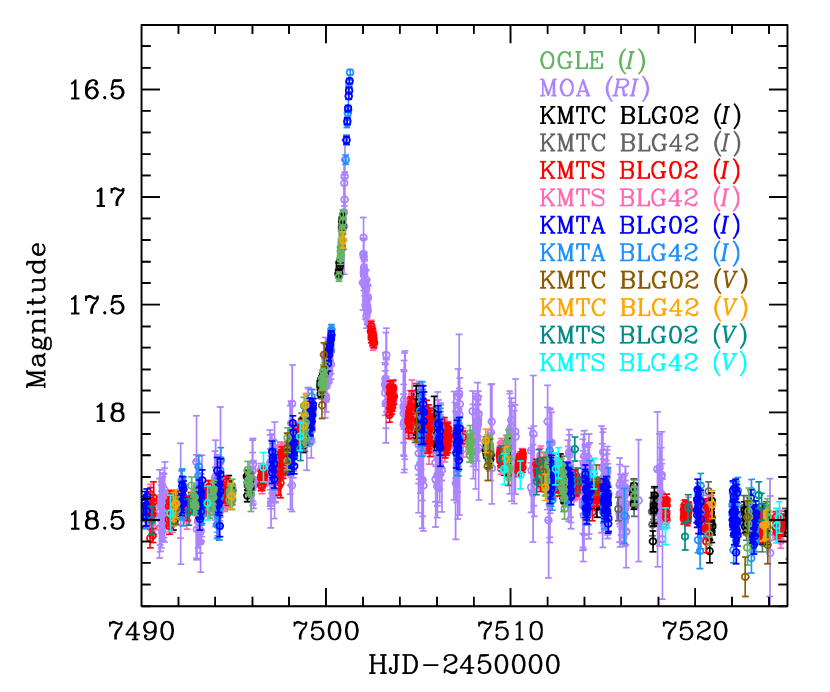
Figure 1.— Light curve of OGLE-2016-BLG-0733. The notation after the each observatory represents the passband of observation.

2. Observation

The equatorial and Galactic coordinates of the microlensing event OGLE-2016-BLG-0733 are $(\alpha,\delta)_{\rm J2000}=(17^{\rm h}55^{\rm m}54^{\rm s}\hskip-2.0pt.29,-29^{\circ}50^{\prime}28^{\prime\prime}\hskip-2.0pt.2)$ and $(l,b)=(0.369^{\circ},-2.388^{\circ})$, respectively. The event was discovered on 2016 Apr 19 UT 19:16 by the Early Warning System (EWS: Udalski et al., 2015) of the OGLE survey, which is conducted using the 1.3m Warsaw telescope located at Las Campanas Observatory in Chile. The MOA survey independently discovered the event using the 1.8m telescope located at Mt. John Observatory in New Zealand. In the MOA lensing event list, it is labeled MOA-2016-BLG-202.

The event was also in the footprint of the KMTNet survey. The KMTNet survey utilizes three identical 1.6m telescopes that are located at Cerro Tololo Interamerican Observatory in Chile (KMTC), South African Astronomical Observatory in South Africa (KMTS), and Siding Spring Observatory in Australia (KMTA). Each of KMTNet telescope is equipped with a $4.0~{}\rm deg^{2}$ camera. With these instruments, the KMTNet survey covers $(12,40,80)~{}\rm deg^{2}$ areas of the Galactic bulge with observation cadences of $(4,\geq 1,\geq 0.4)~{}\rm hr^{-1}$, respectively. For the three major fields covered by a $4~{}\rm hr^{-1}$ cadence, alternating observations cover the sky with a $6^{\prime}$ offset in order to compensate the gap between camera chips. The event lay in one such pair of fields (BLG02 and BLG42) and thus the cadence of the event reached up to $4~{}\rm hr^{-1}$. Combining this feature with its globally distributed telescopes, the KMTNet survey densely and continuously covered the event.

Photometry data used for the analysis were processed using the customized pipelines that are developed by the individual survey groups: Udalski (2003), Bond et al. (2001), and Albrow et al. (2009) for the OGLE, MOA, and KMTNet groups, respectively. These pipelines are based on the Difference Imaging Analysis method (DIA: Alard & Lupton, 1998; Woźniak, 2000; Albrow et al., 2009).

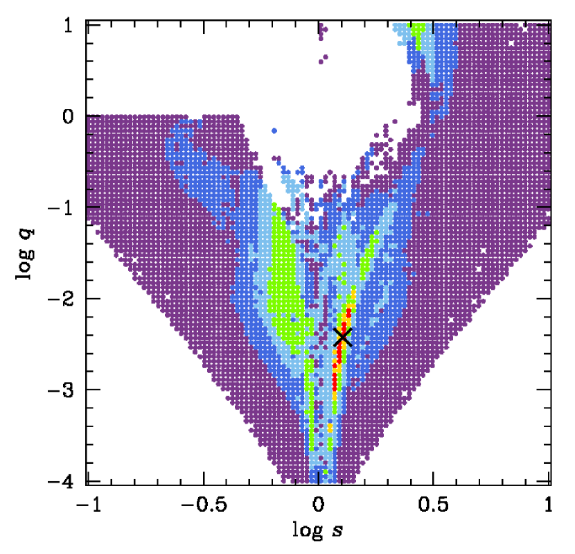
Figure 2.— The $\Delta\chi^{2}$ surface of $(s,q)$ parameter space derived from the initial grid search. Each color represents the contour level of $\Delta\chi^{2}<20\sigma$ (red), $<40\sigma$ (yellow), $<60\sigma$ (green), $<80\sigma$ (light blue), $<100\sigma$ (blue), and $<120{\sigma}$ (purple), respectively. The location of the best-fit solution is marked by the cross symbol.

For the case of KMTNet, data were additionally reduced using the pyDIA software solely to determine the source color. pyDIA is a new modular python package for performing star detection, difference imaging and photometry on crowded astronomical images. For difference imaging, it uses the algorithm of Bramich et al. (2013) with extended delta basis functions that allows independent degrees of control for the differential photometric scaling as well as shape changes of the PSF between images. When available, it uses GPU hardware acceleration for the computationally intensive tasks of difference-imaging and PSF fitting.

A wealth of experience shows that while the error bars reported by microlensing photometry codes are, in general, monotonically related to the true errors, the transformation from one to the other varies from event to event and from observatory to observatory. To compensate for this effect, we renormalize the error bars of the individual data sets by following the method of Yee et al. (2012) with the equation

$$\sigma^{\prime}_{i,j}=\sqrt{\sigma_{\rm min,\it j}^{2}+(k_{j}\sigma_{i,j})^{2}},$$ (1)

where $\sigma_{i,j}$ is the error on the $i$-th point from $j$-th observatory and $\sigma_{\rm min,\it j}$ and $k_{j}$ are the correction parameters for $j$-th observatory. For each data set, we first adjust $\sigma_{\rm min,\it j}$ in order to make the cumulative distribution function of $\chi^{2}$ sorted by lensing magnification linear. Then, we rescale the error bars using $k_{j}$ in order to make $\chi^{2}$ per degree of freedom ($\chi^{2}/{\rm dof}$) unity. Note that the normalization process is conducted based on the best-fit (binary-source) model and we remove $3\sigma$ outliers from the model during the process.

3. Analysis

Analysis of the lensing light curve is carried out by conducting modeling of the observed light curve to find the best-fit lensing parameters. As presented in Figure 1, the light curve of OGLE-2016-BLG-0733 shows deviations from the smooth and symmetric form of an event produced by a single lens. The deviations appear in two regions, one strong anomaly near the peak at ${\rm HJD}^{\prime}(={\rm HJD}-2450000)\sim 7501.4$ and the other weak but long-term anomaly in the falling side of the light curve. Because such deviations are broadly consistent with a binary lens, and because identifying binary and especially planetary lens is a principal goal of micolensing studies, these anomalies triggered a search for binary-lens solutions even before the event returned to baseline. The predictions made by these ongoing “real-time” models were, broadly speaking, confirmed. Although the model nevertheless proves incorrect, we first study how it partially succeeds in explaining the data.

Table 1Lensing Parameters

Parameters	Binary-lens	Binary-source
$\chi^{2}$/dof	12955.8/12347	12411.8/12347
$t_{0,1}$ (${\rm HJD^{\prime}}$)	7501.570 $\pm$ 0.004	7501.374 $\pm$ 0.005
$t_{0,2}$ (${\rm HJD^{\prime}}$)	–	7507.804 $\pm$ 0.116
$u_{0,1}$	0.013 $\pm$ 0.001	0.015 $\pm$ 0.001
$u_{0,2}$	–	0.365 $\pm$ 0.033
$t_{\rm E}$ (days)	27.838 $\pm$ 0.847	14.428 $\pm$ 0.602
$s$	1.281 $\pm$ 0.007	–
$q$ ($10^{-3}$)	3.912 $\pm$ 0.258	–
$\alpha$ (rad)	0.051 $\pm$ 0.001	–
$\rho_{\ast}$ ($10^{-3}$)	8.317 $\pm$ 0.392	–
$q_{F,RI}$	–	2.078 $\pm$ 0.201
$q_{F,I}$	–	1.853 $\pm$ 0.177

Note. — ${\rm HJD}^{\prime}={\rm HJD}-2450000$

3.1. Binary-lens Interpretation

Adopting the parametrization of Jung et al. (2015) for the description of a standard binary-lens light curve, we search for a binary-lens solution by following the method of Jung et al. (2015), one of the well-established modeling procedure developed based on the map-making method (Dong et al., 2006). Figure 2 shows the $\Delta\chi^{2}$ surface of $(s,q)$ parameter space derived from the initial grid search. Here $s$ is the projected binary separation (normalized to the angular Einstein radius of the lens system, $\theta_{\rm E}$) and $q$ $(=M_{2}/M_{1})$ is the mass ratio between the lens components, and they are divided into $100\times 100$ grids in the range of $-1.0<{\rm log}~{}s<1.0$ and $-4.0<{\rm log}~{}q<1.0$, respectively. From the grid search, we find one local minimum. By refining the local solutions, it is found that the best-fit binary-lens model has two masses with a separation $s\sim 1.28$ and a mass ratio $q\sim 0.004$, which would make the companion a planetary-mass object projected near the Einstein radius of its host.

In Table 1, we present the best-fit parameters of the binary-lens solution along with the $\chi^{2}$ values per degree of freedom (dof). The lens system induces two sets of caustics, where one is located near the barycenter of the binary lens and the other is located away from the barycenter between the planet and the host. In Figure 3, we show the light curve of the binary-lens solution in the region of the anomaly and the corresponding geometry of the lens system. We note that the source trajectory in the upper panel is aligned so that the data points marked on the trajectory match those in the lower panel.

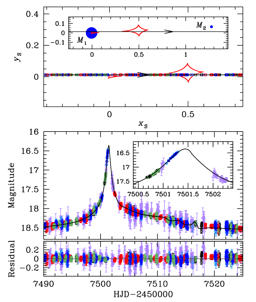
Figure 3.— Geometry and light curve of the binary-lens model. (1) The upper panel shows the geometry of the binary-lens model. The straight line with an arrow is the source trajectory, red closed concave curves represent the caustics, and blue filled circles (marked by $M_{1}$ and $M_{2}$) are the binary-lens components. All length scales are normalized by the Einstein radius. The inset shows the general view and the major panel shows the enlarged view corresponding to the light curve of lower panel. The open circle on the source trajectory is the source position at the time of observation whose size represents the source size. (2) The lower panel shows the enlarged view of the anomaly region. The inset shows a zoom of the light curve near ${\rm HJD}^{\prime}\sim 7501.4$. The curve superposed on the data is the best-fit binary-lens model.

The fit in Figure 3 appears quite good. However, there exists some residuals near the exit of the planetary caustic $7517<{\rm HJD^{\prime}}<7520$. In order to fit the residuals, we additionally test the models considering both the microlens parallax (Gould, 1992, 2004) and the orbital motion of the lens (Dominik, 1998). From this, we find that the introduction of higher-order effects still does not provide a fully acceptable fit. Furthermore, the estimated projected energy ratio between kinetic and potential energy $(\rm KE/\rm PE)_{\bot}=5.77$, in contrast to the requirement that $(\rm KE/\rm PE)_{\bot}<1.0$ to be a bound system (Dong et al., 2009), indicates that the model is physically unrealistic.

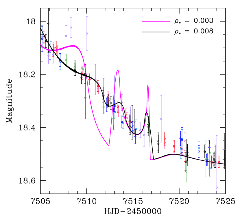
Figure 4.— Comparison of two binary-lens models in the weak anomaly region. The black and magenta curves represent, respectively, the best-fit model and the same model except with a substantially smaller (and more typical) source size $\rho_{*}$. Each data set is binned in time intervals of $24~{}{\rm hr}$, each of which contains a maximum of 10 hrs of contiguous data.

In fact, there are two important clues that this solution is not correct. At first sight these appear to be independent, but are actually closely related. The first is that the normalized source size is very large $\rho_{*}=8\times 10^{-3}$ considering that the source is a dwarf. This would lead to a very small Einstein radius $\theta_{\rm E}\sim 0.05\,$mas and very small lens-source relative proper motion $\mu=\theta_{\rm E}/t_{\rm E}\sim 0.7\,{\rm mas\,yr^{-1}}$, where $t_{\rm E}$ is the Einstein time scale. As discussed in Penny et al. (2016), where they presented the combination of $\mu$ and $\theta_{\rm E}$ for Galactic microlensing events using the model of Henderson et al. (2014), these values are a priori extremely unlikely, although not impossible: they could be generated by a very slow lens at a distance $D_{\rm LS}\sim 20\,{\rm pc}(M/M_{\odot})^{-1}$ in front of the source.

What raises this suspiciously large $\rho_{*}$ to the level of implausibility is that it appears to be “driven” by the need to match basically smooth data to an intrinsically “bumpy” model. Because the source crossing time $t_{*}\equiv\rho_{*}t_{\rm E}\sim 5\,$hr is similar to the duration of an observing night, it is appropriate to bin these data by observatory and by day. Figure 4 compares these binned data to the best-fit model and also to the same model but with a more typical value of $\rho_{*}=3\times 10^{-3}$. This shows that the data are much smoother than the model for a typical $\rho_{*}$ and are still considerably smoother than the model for the best-fit $\rho_{*}$. We therefore are led to consider what other physical effects might generate this “planetary” anomaly.

3.2. Binary-source Interpretation

We consider the possibility that the long-term deviation may be caused by a single-lens event with a binary source. In case of a binary-source event, the lensing magnification corresponds to the superposition of the two single-source events generated by the individual source stars (Griest & Hu, 1992; Han, 2002), i.e.

$$A={A_{1}F_{1}+A_{2}F_{2}\over F_{1}+F_{2}}={A_{1}+q_{F}A_{2}\over 1+q_{F}},$$ (2)

where $A_{i}$ denotes the lensing magnification of each source star with a flux $F_{i}$ and $q_{F}=F_{2}/F_{1}$ is the flux ratio between the two source stars. In contrast to a single-source magnification, the total magnification $A$ is wavelength dependent because the different colors between two sources can induce a color change during the course of the lensing phenomenon.

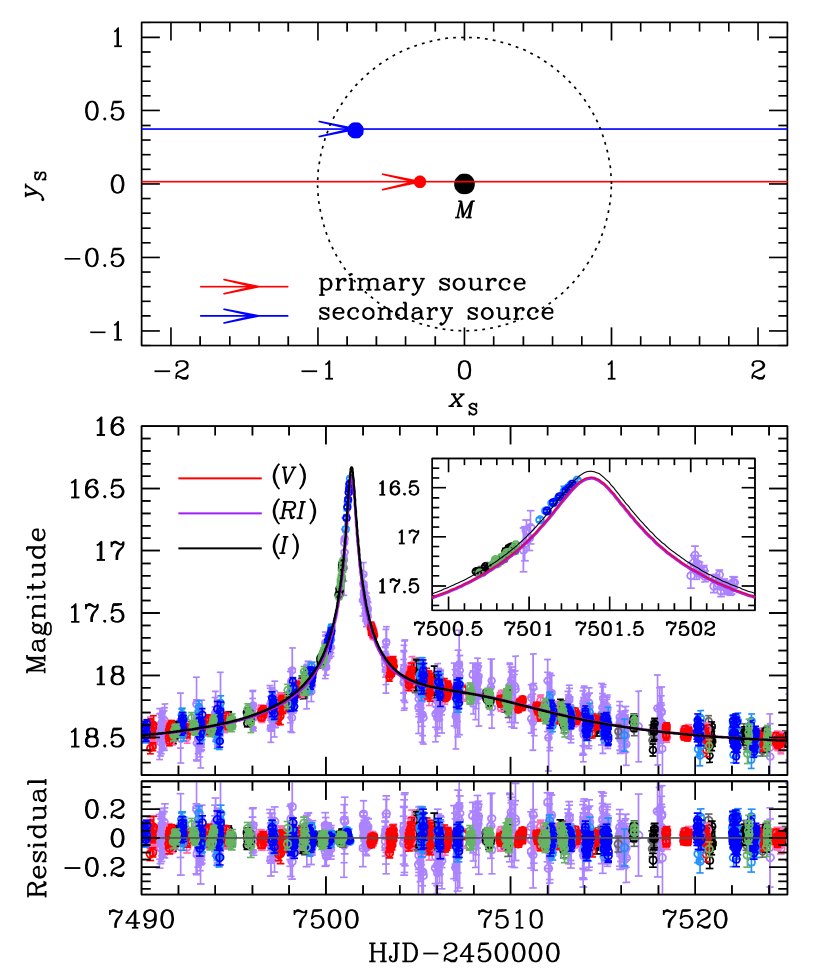
Figure 5.— Geometry and light curve of the binary-source model. (1) The upper panel shows the geometry of the binary-source model. Two straight lines with arrows are the source trajectories of individual source stars. The lens is located at the origin (marked by $M$), and the dotted circle is the angular Einstein ring. The red and blue filled circles represent the individual source positions at ${\rm HJD}^{\prime}=7497$. Lengths are normalized by the Einstein radius. (2) The lower panel shows the enlarged view of the anomaly region. The two curves with different colors are best-fit binary-source models for $RI$ and $I$ passbands. The inset shows a zoom of the anomaly near ${\rm HJD}^{\prime}\sim 7501.4$. We note that, although we only use the $V$ band data for determining the source type, we also present the $V$ band model light-curve to compare the color change between passbands.

Under the approximation that the transverse speeds of the two sources with respect to the lens are same, the single-source magnification is related to the lens-source separation normalized to the angular Einstein radius, $u_{i}$, by

$$A_{i}={u_{i}^{2}+2\over u_{i}\sqrt{u_{i}^{2}+4}};\qquad u_{i}(t)=\left[\left({t-t_{0,i}\over t_{\rm E}}\right)^{2}+u_{0,i}^{2}\right]^{1/2},$$ (3)

where $t_{0,i}$ is the moment of the closest lens approach to each source star, $u_{0,i}$ denotes the separation between the lens and individual sources at $t_{0,i}$, and $t_{\rm E}$ is the timescale required for the source to cross the angular Einstein radius (Einstein time scale). Therefore, one needs 6 principal parameters $(t_{0,1},t_{0,2},u_{0,1},u_{0,2},t_{\rm E},q_{F})$ for the description of a standard binary-source event. Since the flux ratio varies depending on the passband, one must add additional flux ratio parameters for each of the observed passbands. We note that, due to the unknown sign of $u_{0,i}$, the binary-source interpretation suffers a similar degeneracy to the well-known satellite parallax degeneracy (Refsdal, 1966; Gould, 1994), resulting in four degenerate solutions that are generally denoted by $(+,+)$, $(-,-)$, $(+,-)$, and $(-,+)$, where the two signs in the parenthesis indicate the sign of $u_{0,1}$ and $u_{0,2}$, respectively.

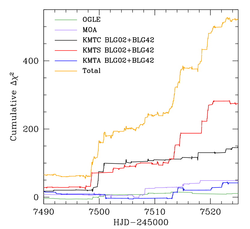
Figure 6.— Cumulative distribution of $\chi^{2}$ difference between the binary-source and binary-lens models.

The four-fold degeneracy introduces a two-fold degeneracy in the measurement of the source plane Einstein radius $\hat{r}_{\rm E}$, defined by

$$\hat{r}_{\rm E}=D_{\rm S}\theta_{\rm E}=r_{\rm E}{D_{\rm S}\over D_{\rm L}}.$$ (4)

Here $r_{\rm E}={D_{\rm L}}{\theta_{\rm E}}$ is the physical Einstein radius, $D_{\rm S}$ and $D_{\rm L}$ are the distance to the source and the lens, respectively. The physical projected separation between the sources, $d_{\rm s}$, is related to $\hat{r}_{\rm E}$ by

$$d_{\rm s}={\hat{r}_{\rm E\pm}}\left[\left({\Delta}{t_{0}}\over{t_{\rm E}}\right)^{2}+{\Delta}{u_{0}}^{2}\right]^{1/2},$$ (5)

where ${\Delta}{t_{0}}=|t_{0,1}-t_{0,2}|$, and ${\Delta}{u_{0}}=|u_{0,1}\pm u_{0,2}|$. Therefore, if the separation $d_{\rm s}$ is measured from follow-up spectroscopic observation of the sources, the Einstein radius is determined with two possible values of $\hat{r}_{\rm E\pm}$ depending on ${\Delta}{u_{0}}$ (Han & Gould, 1997).

The transverse speeds of the two sources can be different when the orbital motion of the binary source is substantial (“source orbit”). In this case, the positions of the individual sources are described by the summation of the rectilinear motion of the barycenter of the binary source (CM) and the orbital motion of the sources with respect to the CM. Similar to the effect of the binary-lens orbital motion (Dominik, 1998; Jung et al., 2013), the “source orbit” effect also causes the angle between the trajectory of the CM and the binary-source axis ${\alpha_{\rm s}}$ and the projected separation between the source components $s_{\rm s}$ (normalized to $\theta_{\rm E}$) to change in time. To first-order approximation, the source-orbital motion can be parameterized as $ds_{\rm s}/dt$ and $d{\alpha_{\rm s}}/dt$ which represent the change rate of the binary-source separation and the orientation angle, respectively. Then, the binary-source separation and the orientation angle at time $t$ are

$$s_{\rm s}^{\prime}=s_{\rm s}+{ds_{\rm s}\over dt}(t-t_{\rm ref}),\qquad\alpha_{\rm s}^{\prime}=\alpha_{\rm s}+{d{\alpha_{\rm s}}\over dt}(t-t_{\rm ref}),$$ (6)

where $t_{\rm ref}$ is the reference time for the binary-source orbital motion. The positions of the two sources on the lens plane are thus

$$u_{i}^{2}(t)=\left[\left({t-t_{0}\over t_{\rm E}}\right)\pm s_{\rm s,\it i}\,{\rm cos}\,{\alpha_{\rm s}^{\prime}}\right]^{2}+\left(u_{0}\mp s_{\rm s,\it i}\,{\rm sin}\,{\alpha_{\rm s}^{\prime}}\right)^{2},$$ (7)

where $s_{\rm s,1}=s_{\rm s}^{\prime}q_{\rm s}/(1+q_{\rm s})$ and $s_{\rm s,2}=s_{\rm s}^{\prime}/(1+q_{\rm s})$ are the separation between the two sources and the CM, and $q_{\rm s}=M_{\rm s,2}/M_{\rm s,1}$ is the mass ratio between the source components. Here the parameters $(t_{0},u_{0},t_{\rm E})$ describe the relative motion between the lens and the CM. As a result, one requires 9 principal parameters $(t_{0},u_{0},t_{\rm E},s_{\rm s},q_{\rm s},\alpha_{\rm s},ds_{\rm s}/dt,d\alpha_{\rm s}/dt,q_{F})$ to describe the orbital motion of the binary source.

We separately test “standard” and “source orbit” models. In the “source orbit” model, we test four degenerate solutions resulting from the unknown sign of $u_{0,i}$. We investigate the solution of the parameters by a downhill approach. The initial values of the parameters are set based on the peak time, magnification, and duration of the event. We adopt the Markov Chain Monte Carlo (MCMC) method for the $\chi^{2}$ minimization of the downhill approach.

From the comparison between the “standard” and the “source orbit” models, it is found that the orbital motion of the binary source does not improve the fit significantly. The $\chi^{2}$ difference between the “standard” and each “source orbit” model is very low $(\Delta\chi^{2}<1)$. Consequently, the measured values of two orbital parameters $(ds_{\rm s}/dt,d\alpha_{\rm s}/dt)$ are consistent with zero in all four “source orbit” solutions. These imply that the light curve of the event does not have sufficient information for constraining the orbital parameters (see the Appendix of Han et al. 2016 for a detailed review). We therefore only consider the “standard” model.

We find that the binary-source interpretation provides a good fit to the observed light curve. In Table 1, we summarize the best-fit parameters of the binary-source solution. In Figure 5, we show the geometry of the relative lens-source motion (upper panel) and the model light curve (lower panel) of the binary-source solution. In the upper panel, the two lines with arrows represent the trajectories of the two source stars with respect to the lens (marked by “$M$”). We designate the source passing closer to the lens as the “primary” source and the other source as the “secondary” source. We find that the flux ratio ($q_{F,RI}=2.0$ and $q_{F,I}=1.9$) is greater than unity, indicating that the source approaching closer to the lens is fainter than the source approaching farther from the lens. While binary-lens light curves are almost perfectly achromatic (after subtraction of the blended light), binary-source event light curves can be chromatic, implying that the magnification varies depending on the observed passband, and thus we present two model light curves corresponding to $RI$ band (MOA) and $I$ band (the other groups) data sets. According to the binary-source interpretation, the strong anomaly near the peak was produced when the fainter source star approached close to the lens and the anomaly in the declining wing was produced when the brighter source approached.

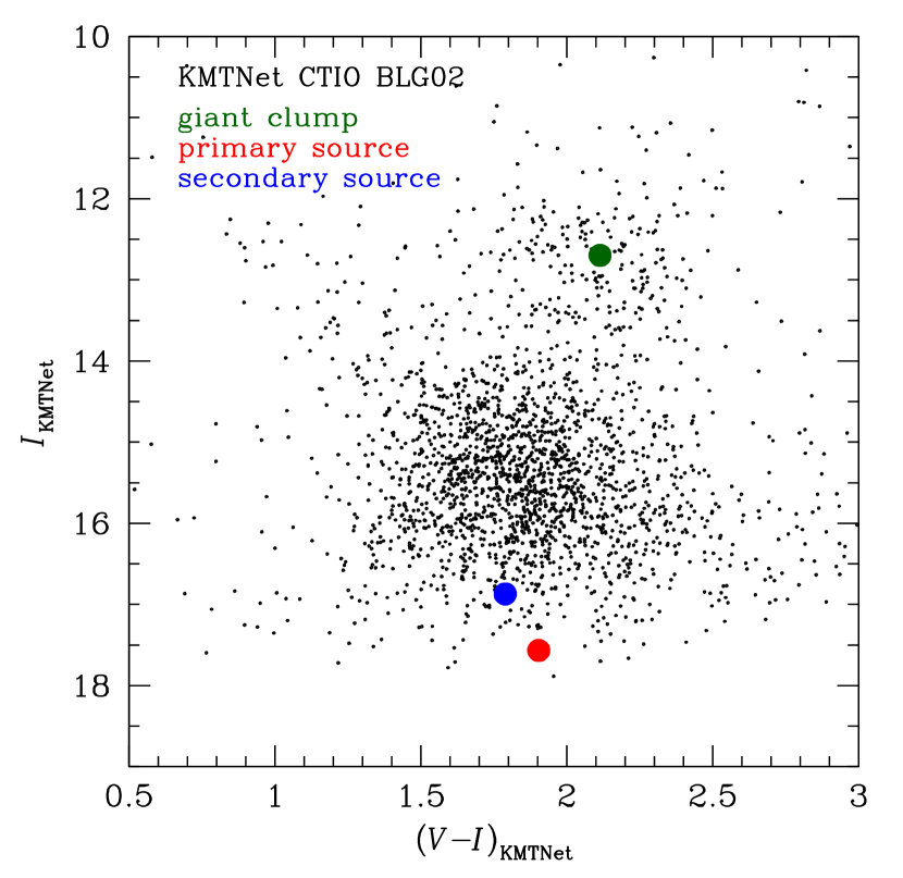
Figure 7.— Instrumental color-magnitude diagram of stars in the region around the source stars. The positions of individual source components and the centroid of the giant clump are marked.

By comparing the binary-lens and binary-source interpretations, we find that the binary-source model better explains the observed light curve. The binary-source model improves the fit by $\Delta\chi^{2}\sim 544$ compared to the binary-lens model. In Figure 6, we present the cumulative distribution of $\Delta\chi^{2}$ of the binary-source model with respect to the binary-lens model as a function of time. This shows that the major improvements occur during the ascending part of the strong anomaly near $7498<{\rm HJD^{\prime}}<7501$ and the descending part of the light curve near $7514<{\rm HJD^{\prime}}<7520$, where the KMTNet survey densely and continuously covers the anomaly. The fit improvement from KMTNet data is $\Delta\chi^{2}\sim 484$. This demonstrates the importance of the high-cadence observation for the unambiguous characterization of the lensing event.

3.3. Source Type

Knowing that OGLE-2016-BLG-0733 is better explained by the binary-source interpretation, we characterize the individual source stars by estimating the source type from the de-reddened color $(V-I)_{0}$ and brightness $I_{0}$. For this, we use four KMTNet pyDIA reductions ([CTIO+SAAO]$\times$[BLG02+BLG42]) to construct the instrumental color-magnitude diagrams (CMD). Based on the method of Yoo et al. (2004), we first estimate the offsets in color $\Delta(V-I)$ and magnitude $\Delta{I}$ between individual sources and the centroid of giant clump (GC). Figure 7 shows the instrumental CMD of one of four KMTNet fields (CTIO BLG02) where the locations of individual sources and GC are shown. Assuming that the source and GC suffer the same extinction combined with the known de-reddened color $(V-I)_{0,\rm GC}=1.06$ and magnitude $I_{0,\rm GC}=14.43$ of GC (Bensby et al., 2011; Nataf et al., 2013), we then estimate the de-reddened color and magnitude of the individual sources. By applying this procedure to each KMTNet field, we find that the mean de-reddened color and magnitude of the individual sources are $(V-I,I)_{0,1}=(0.79\pm 0.10,19.32\pm 0.05)$ for the primary and $(V-I,I)_{0,2}=(0.68\pm 0.07,18.63\pm 0.03)$ for the secondary. These correspond to a late and an early G-type main-sequence star for the primary and the secondary, respectively.

Note that we also characterize the source star based on the binary-lens interpretation solely for the purpose of incorporating the limb-darkening coefficients into the binary-lens model. By following the same procedure, we determine the mean de-reddened color and magnitude of the source as $(V-I,I)_{0}=(0.76\pm 0.08,19.60\pm 0.05)$ corresponding to a G-type main-sequence star.

4. Discussion

For the great majority of microlensing planets published to date (see Mróz et al. 2016 for a recent listing), the light curves exhibit sharp caustic crossings indicative of a binary lens. While in some cases there is difficulty in establishing whether the companion is planetary or has a more-equal mass ratio, this potential ambiguity is decisively resolved in almost all cases.

However, a high-cadence round-the-clock survey (such as those reported here) is capable of detecting much subtler planetary signals than those published to date. Furthermore, such a survey enables a complete statistical analysis that addresses all possible planetary signals rather than just individual detections. At the same time, Zhu et al. (2014a, b) have shown that of order half of the planets detectable will lack caustic crossing features. Hence, the problem of distinguishing such planetary light curves from other physical effects will be much more challenging than in the past, but extremely important for interpreting statistical results about planet populations.

Here we have presented the first of a new class of potential planet impersonators: roughly equal-luminosity binary source events, with the two sources having a factor of two flux difference and being separated by substantially less than an Einstein radius. This can be regarded as a form of the degeneracy proposed by Gaudi (1998) in the sense that a binary source is masquerading as a planet. However, it lies quite far in parameter space from the original Gaudi degeneracy from the standpoint both of the physical nature of the binary source and the characteristics of the planetary light curve that are being imitated. For the Gaudi degeneracy, the second source is much fainter than the first and should be separated by of order an Einstein radius or more. In this way, the perturbation can appear to be short, and its symmetric form will not conflict with asymmetries of planetary perturbations generated by planets with projected separations near the Einstein ring. By contrast, the binary-source system of OGLE-2016-BLG-0733 has roughly equal brightness and so induces broad perturbations to the light curve, which are then confused with a broadened central peak and large planetary deviation, which are characteristic of a planet near the Einstein ring.

We found that, once binary-source models were investigated, it was quite easy to see that it is preferred over the binary-lens model with $\Delta\chi^{2}\sim 500$. Moreover, the planetary model exhibited “suspicious” behavior, which is what led us to investigate the binary source model. Thus, it may seem that there is no reason to worry that this could be an extension of the Gaudi degeneracy (or any kind of degeneracy at all). However, unambiguously distinguishing between these two classes of models was dependent on having high-cadence data, which may not be available in all cases. Furthermore, in the future, a blind search for planetary signals will not turn up all potential competing models unless those models are specifically considered. The microlensing event OGLE-2016-BLG-0733 demonstrates another, previously unknown, potential ambiguity that could confuse systematic analyses of microlensing planetary signals.

References

- Alard & Lupton (1998) Alard, C., & Lupton, Robert H. 1998, ApJ, 503, 325
- Albrow et al. (2009) Albrow, M. D., Horne, K., Bramich, D. M., et al. 2009, MNRAS, 397, 2099
- Alcock et al. (1993) Alcock, C., Akerlof, C. W., Allsman, R. A., et al. 1993, Nature, 365, 621
- Bensby et al. (2011) Bensby, T., Adén, D., Meléndez, J., et al. 2011, A&A, 533, 134
- Bond et al. (2001) Bond, I. A., Abe, F., Dodd, R. J., et al. 2001, MNRAS, 327, 868
- Bond et al. (2004) Bond, I. A., Udalski, A., Jaroszyński, M., et al. 2004, ApJ, 606, 155
- Bozza et al. (2016) Bozza, V., Shvartzvald, Y., Udalski, A., et al. 2016, ApJ, 820, 79
- Bramich et al. (2013) Bramich, D. M., Horne, K., Albrow, M. D., et al. 2013, MNRAS, 428, 2275
- Choi et al. (2012) Choi, J.-Y., Shin, I.-G., Han, C., et al. 2012, ApJ, 756, 48
- Claret (2000) Claret, A. 2000, A&A, 363, 1081
- Dominik (1998) Dominik, M. 1998, A&A, 329, 361
- Dong et al. (2006) Dong, S., Depoy, D. L., Gaudi, B. S., et al. 2006, ApJ, 642, 842
- Dong et al. (2009) Dong, S., Gould, A., Udalski, A., et al. 2009, ApJ, 695, 970
- Erdl & Schneider (1993) Erdl, H., & Schneider, P. 1993, A&A, 268, 453
- Gaudi (1998) Gaudi, B. S. 1998, ApJ, 506, 533
- Gaudi (2012) Gaudi, B. S. 2012, ARA&A, 50, 411
- Gould (1992) Gould, A. 1992, ApJ, 392, 442
- Gould (1994) Gould, A. 1994, ApJ, 421, 75
- Gould (2004) Gould, A. 2004, ApJ, 606, 319
- Gould & Loeb (1992) Gould, A., & Loeb, A. 1992 ApJ, 306, 104
- Gould et al. (2013) Gould, A., Yee, J. C., Bond, I. A., et al. 2013, ApJ, 763, 141
- Griest & Hu (1992) Griest, K., & Hu, W. 1992, ApJ, 397, 362
- Han (2002) Han, C. 2002, ApJ, 564, 1015
- Han & Gould (1997) Han, C. & Gould, A. 1997, ApJ, 480, 196
- Han et al. (2016) Han, C., Udalski, A., Gould, A., et al. 2016, ApJ, 828, 53
- Henderson et al. (2014) Henderson, C. B., Gaudi, B. S., Han, C., et al. 2014, ApJ, 794, 52
- Hwang et al. (2013) Hwang, K.-H., Choi, J.-Y., Bond, I. A., et al. 2013, ApJ, 778, 55
- Jung et al. (2013) Jung, Y. K., Han, C., Gould, A., & Maoz, D. 2013, ApJ, 768, L7J
- Jung et al. (2015) Jung, Y. K., Udalski, A., Sumi, T., et al. 2015, ApJ, 798, 123
- Kim et al. (2016) Kim, S.-L., Lee, C.-U., Park, B.-G., et al. 2016, JKAS, 49, 37
- Mao & Paczyński (1991) Mao, S., & Paczyński, B. 1991 ApJ, 517, L35
- Mróz et al. (2016) Mróz, P., Han, C., Udalski. A., et al. 2016, arXiv:1607.04919
- Nataf et al. (2013) Nataf, D. M., Gould, A., Fouqué, P., et al. 2013, ApJ, 769, 88
- Paczyński (1986) Paczyński, B. 1986, ApJ, 304, 1
- Penny et al. (2016) Penny, M. T., Henderson, C. B., & Clanton, C. 2016, ApJ, 830, 150
- Refsdal (1966) Refsdal, S. 1966, MNRAS, 134, 315
- Sako et al. (2008) Sako, T., Sekiguchi, T., Sasaki, M., et al. 2008, ExA, 22, 51
- Schneider & Weiss (1986) Schneider, P., & Weiss, A. 1986, A&A, 164, 237
- Spergel et al. (2015) Spergel, D., Gehrels, N., Baltay, C., et al. 2015, arXiv:1503.03757
- Udalski et al. (1993) Udalski, A., Szymanski, M., Kaluzny, J., et al. 1993, Acta Astron., 43, 28
- Udalski (2003) Udalski, A. 2003, Acta Astron., 53, 291
- Udalski et al. (2015) Udalski, A., Szymański, M. K., & Szymański, G. 2015, Acta Astron, 65, 1
- Woźniak (2000) Woźniak, P. R. 2000, Acta Astron., 50, 42
- Yee et al. (2012) Yee, J. C., Shvartzvald, Y., Gal-Yam, A., et al. 2012, ApJ, 755, 102
- Yoo et al. (2004) Yoo, J., DePoy, D. L., Gal-Yam, A., et al. 2004, ApJ, 603, 139
- Zhu et al. (2014a) Zhu, W., Gould, A., Penny, M., Mao, S., & Gendron, R. 2014, ApJ, 794, 53
- Zhu et al. (2014b) Zhu, W., Penny, M., Mao, S., Gould, A., & Gendron, R. 2014, ApJ, 788, 73