Surface effects on ferromagnetic resonance in magnetic nanocubes

Abstract

We study the effect of surface anisotropy on the spectrum of spin-wave excitations in a magnetic nanocluster and compute the corresponding absorbed power. For this, we develop a general numerical method based on the (undamped) Landau-Lifshitz equation, either linearized around the equilibrium state leading to an eigenvalue problem or solved using a symplectic technique. For box-shaped clusters, the numerical results are favorably compared to those of the finite-size linear spin-wave theory. Our numerical method allows us to disentangle the contributions of the core and surface spins to the spectral weight and absorbed power. In regard to the recent developments in synthesis and characterization of assemblies of well defined nano-elements, we study the effects of free boundaries and surface anisotropy on the spin-wave spectrum in iron nanocubes and give orders of magnitude of the expected spin-wave resonances. For an $8\ {\rm nm}$ iron nanocube, we show that the absorbed power spectrum should exhibit a low-energy peak around 10 GHz, typical of the uniform mode, followed by other low-energy features that couple to the uniform mode but with a stronger contribution from the surface. There are also high-frequency exchange-mode peaks around 60 GHz.

1 Introduction

During the last decades the development of potential technological applications of magnetic nanoparticles, such as magnetic imaging and magnetic hyperthermia, has triggered a new endeavor for a better control of the relevant properties of such systems. In particular, synthesis and growth of crystalline nanoparticles have reached such a high level of skill and know-how as to produce well defined $2D$ and $3D$ arrays of nanoclusters of tailored size, shape and internal crystal structure [1, 2, 3, 4, 5, 6]. On the other hand, experimental measurements on nanoscale systems are a step behind inasmuch as they still do not provide us with sufficient space-time resolutions for an unambiguous interpretation of the observed phenomena that are commonly attributed to finite-size or surface effects. Nonetheless, ferromagnetic resonance (FMR), which is a well known and very precise technique for characterizing bulk and layered magnetic media [7, 8, 9], benefits from a renewed interest in the context of nanomagnetism. Indeed, some newly devised variants of the FMR technique [10, 11, 12, 13, 14, 15] combine the study of dynamic magnetic properties by FMR with the elemental specificity of the chemical composition of the particles. For instance, these techniques can be employed to detect the ferromagnetic resonance of single Fe nanocubes with a sensitivity of $10^{6}\mu_{\mathrm{B}}$ and element-specific excitations in Co-Permalloy structures. Another variant of ferromagnetic resonance spectroscopy is the so-called Magnetic Resonance Force Microscopy (MRFM)[16]. It has recently been used for the characterization of cobalt nanospheres [17]. These techniques hold the prospect of providing a better resolution of the surface properties at the level of a single (isolated) magnetic nanoparticle. For the benefits of theoretical work, these experiments could provide the missing data for resolving the surface response to a time-dependent magnetic field, and thus contribute to assess the validity of surface-anisotropy models. In particular, measurements of the absorbed power in FMR experiments on “isolated” particles or dilute assemblies of nanoparticles could serve these purposes. Indeed, this is a standard observable that is routinely measured in such experiments. From the theory standpoint, it is a well known (dynamic) response of a magnetic system that can be computed by various well established techniques, analytical as well as numerical.

In the present work we consider a box-shaped nanocluster modeled as a many-spin system with free boundary conditions, subjected to a time-dependent (small-amplitude) magnetic field. The systems considered here are chosen to model, to some extent, Fe nanocubes studied by several groups [3, 10, 18, 5, 6]. Our main objective is to distinguish and assess the role of surface and core contributions to the FMR absorption spectra. For this we focus on the simple system of an isolated (ferromagnetic) nanocube and study its intrinsic properties, thus ignoring its interactions with other nanocubes that would be included in an assembly and its interactions with the hosting matrix. As shown by Sukhov et al. [19], this assumption is fully justified in the case of dilute samples. Obviously, real systems of magnetic nanoparticles are far more complex. Indeed, Fe nanoparticles may present a variety of morphologies and internal structures, especially in a core/shell configuration where one observes an antiferromagnetic layer coating a ferromagnetic system [20, 21, 22]. However, the system we adopt is simple enough to illustrate our study in a clear manner but rich enough to capture the main physics we are interested in. Furthermore, the methods we develop here are quite versatile and can be extended to a given magnetic nanoparticle with arbitrary physical parameters.

Consequently, the energy of the nanocluster considered here includes the Zeeman energy, the (nearest-neighbor) spin-spin exchange coupling and on-site anisotropy (core and surface). We also allow for the possibility that exchange interactions involving one or more sites in the surface outer shell to be different from those in the core or at the interface between the core and the surface. Upon solving the (undamped) Landau-Lifshitz equation (LLE) we compute the absorbed power of such systems. Then, the LLE equation is linearized around the equilibrium state of lowest energy and the ensuing eigenvalue problem is solved to infer the full spectrum (eigenfrequencies and eigenfunctions) of all spin-wave excitations. Finally, by comparison with the absorbed power of a given mode, we can determine the separate contributions of core and surface of the nanocluster.

The paper is organized as follows : in the next Section we present our model and computing methods. We give the model Hamiltonian and then describe the two numerical methods we used to compute the full spin-wave spectrum (eigenfrequencies and eigenvectors) and the absorbed power. In Section III we present and discuss our results for the effects of size and surface anisotropy on the absorbed power. This section ends with a discussion of Fe nanocubes for which we give orders of magnitude and speculate on the possibility to observe the calculated peak in the absorbed power. An appendix has been added on a toy model of a three-layer system in order to illustrate, in a simpler manner, how the various branches in the spin-wave dispersion can be associated with spins of a given type (core or surface) in the system.

2 Model and Methods

2.1 The Hamiltonian

We model the magnetic nanocluster as a system of $\mathcal{N}$ classical spins $\mathbf{s}_{i}$, with $|\mathbf{s}_{i}|=1$, with the help of the Hamiltonian

$$\mathcal{H}=\mathcal{H}_{{\rm ex}}+\mathcal{H}_{{\rm an}},$$ (1)

where

$$\mathcal{H}_{{\rm ex}}=-\frac{1}{2}\sum_{i,j}J_{ij}\mathbf{s}_{i}\cdot\mathbf{s}_{j}$$ (2)

is the ferromagnetic Heisenberg exchange interaction and $\mathcal{H}_{{\rm an}}$ the anisotropy contribution. We assume only nearest-neighbor interactions (nn), $J_{ij}=J>0$ for $i,j\in\mathrm{nn}$ and zero otherwise. However, we use a numerical method that allows us to consider different exchange couplings between the core and surface spins according to their loci. More precisely, we may distinguish between core-core ($J_{c}$), core-surface ($J_{cs}$) and surface-surface ($J_{s}$) exchange coupling. The anisotropy term in Eq. (1) is assumed to be uniaxial (along the $z$ axis) with constant $D>0$ for core spins and of Néel’s type with constant $D_{S}$ for surface spins. More precisely, the anisotropy energy is local (on-site), so that $\mathcal{H}_{{\rm an}}=\sum_{i}\mathcal{H}_{{\rm an},i}$, and given by

$$\mathcal{H}_{{\rm an},i}=\left\{\begin{array}[]{lc}-D\left(\mathbf{s}_{i}\cdot\mathbf{e}_{z}\right)^{2},&i\in\mathrm{core}\\ \\ \frac{1}{2}D_{S}{\displaystyle\sum_{j\in\mathrm{nn}}}\left(\mathbf{s}_{i}\cdot\mathbf{u}_{ij}\right)^{2},&i\in\mathrm{surface}.\end{array}\right.$$ (3)

Here $\mathbf{u}_{ij}$ is the unit vector connecting the surface site $i$ to its nearest neighbor on site $j$. Néel’s anisotropy arises due to missing nearest neighbors for surface spins. In particular, for the simple cubic lattice and $xy$ surfaces (perpendicular to the $z$ axis), the Néel anisotropy becomes $\mathcal{H}_{{\rm an},i}=-\frac{1}{2}D_{S}s_{i,z}^{2}$. This means that for $D_{S}>0$ the spins tend to align perpendicularly to the surface, while for $D_{S}<0$ the surface spins tend to align in the tangent plane. In a box-shaped nanocluster the Néel anisotropy on the edges along the $z$ axis becomes $\mathcal{H}_{{\rm an},i}=-\frac{1}{2}D_{S}\left(s_{i,x}^{2}+s_{i,y}^{2}\right)$ or, equivalently, $\mathcal{H}_{{\rm an},i}=\frac{1}{2}D_{S}s_{i,z}^{2}$. As such, for $D_{S}>0$ the edge spins tend to align perpendicularly to the edges. On the other hand, it is easy to check that Néel’s anisotropy vanishes at the corners and in the core of a box-shaped nanocluster.

For the sake of simplicity, and for an easier comparison with experiments on iron nanocubes, for instance, the systems investigated in the present work are boxed-shaped with $\mathcal{N}=N_{x}\times N_{y}\times N_{z}$ with a simple cubic lattice. In this case, the surface anisotropy (SA) favours an ordering along the shortest edges of the particle if $D_{S}>0$ and along the longest ones otherwise. Indeed, for an atom on the edge in the $x$ direction, for instance, we have $4$ neighbors with $\mathbf{u}_{ij}=\mathbf{e}_{x},\mathbf{u}_{ij}=-\mathbf{e}_{x},\mathbf{u}_{ij}=\mathbf{e}_{y},\mathbf{u}_{ij}=-\mathbf{e}_{z}$ and thereby (using $|\mathbf{s}_{i}|=1$) we obtain $\mathcal{H}_{{\rm an},i}\rightarrow\frac{D_{S}}{2}+\frac{D_{S}}{2}\,s_{i,x}^{2}$.

2.2 Excitation spectrum and absorbed power: computing methods

Since surface anisotropy is much stronger than the core anisotropy and the fraction of surface spins for nanoclusters is appreciable, SA strongly influences the spin-wave spectrum of the cluster. Experimentally, the most accessible modes are the spin-wave modes that couple to the uniform ac field, as in magnetic-resonance experiments. In the absence of SA, only the uniform-precession mode is seen in the magnetic resonance. The effect of SA is twofold. First, the uniform (or nearly uniform) precession frequency is modified by SA; it increases or decreases depending on geometry. Hence, combining magnetic-resonance experiments with the corresponding theoretical results provides a means for estimating the surface-anisotropy constant. Second, in larger clusters exchange stiffness becomes less restrictive and different groups of spins (such as the core and surface spins) can precess at different frequencies and this leads to several resonance peaks.

In this Section we describe two complementary methods we have used to compute the spin-wave spectrum and the absorbed power. The first method consists in linearizing the (undamped) Landau-Lifshitz equation (LLE) around the equilibrium position and then solving the ensuing eigenvalue problem to obtain the eigenfrequencies and the corresponding eigenvectors (spin-wave modes). This method is quite versatile as it can be applied to any nanocluster with arbitrary size, shape and energy parameters. In the case of box-shaped nanoclusters this method is compared with the results of linear spin-wave theory obtained in Refs. [23, 24]. The second numerical method used here consists in directly solving the LLE using the technique of symplectic integrators [25, 26]. As will be seen later these two methods are in a very good agreement.

2.2.1 Linearization of the Landau-Lifshitz equation: normal modes of a nanocluster

Here we deal with the numerical solution of the Landau-Lifshitz equation (LLE) of motion

$$\hbar\frac{d{\bf s}_{i}}{dt}={\bf s}_{i}\times\mathbf{H}_{\mathrm{eff},i}-\lambda\,{\bf s}_{i}\times\left({\bf s}_{i}\times\mathbf{H}_{\mathrm{eff},i}\right),$$ (4)

where the effective field is defined by $\mathbf{H}_{\mathrm{eff},i}=-\delta_{\mathbf{s}_{i}}\mathcal{H}+g\mu_{B}\mathbf{H}(t)$, with $g$ being the Landé factor and $\mu_{B}$ the Bohr magneton, $\lambda$ the dimensionless damping parameter and $\mathbf{H}(t)$ the time-dependent magnetic field. In the following we set $\lambda=0$ (Larmor equation) to avoid artificial effects. Internal spin-wave processes in the particle can provide a natural damping of spin waves, especially for larger particles and non-zero temperatures. For nanosize particles, spin-wave modes are essentially discrete [23, 24], while damping requires quasi-continuous excitation branches to satisfy energy conservation in spin-wave processes. In addition, we do not include thermal excitation via stochastic Langevin fields in the model. Thus we expect that the spin wave modes of our particles are undamped. In other words, in this work, we are not seeking the precise result for the microwave absorption. We use these calculations to find positions of spin-wave peaks and compare them with a second approach. Our numerical experiment is short-time whereas damping comes into play at longer times that we are not considering here.

One of the goals of the present work is to assess the role of the surface contribution to the energy spectrum of a single nanocluster or to a given physical observable that is easily accessible experimentally, e.g. the absorbed power. So, before we compute the relevant observable, it is necessary to compute the eigenvectors and eigenenergies of the system. Then, it is our aim to try to attribute the various peaks in the energy spectrum to the core or surface contributions and to estimate the corresponding statistical weight. The eigenvalue problem by linearizing the LLE (4) around the equilibrium state $\left\{{\bf s}_{i}^{(0)}\right\}_{i=1,\ldots,\mathcal{N}}$. This has been done in the system of spherical coordinates in order to reduce the number of equations from $3\mathcal{N}$ to $2\mathcal{N}$. The main steps of our formalism are summarized in A. More precisely, we write $\delta{\bf s}_{i}={\bf s}_{i}-{\bf s}_{i}^{(0)}$, for $i=1,\ldots,\mathcal{N}$, and expand the first derivative of the energy $\mathcal{E}$ (or the effective field) to $1^{\mathrm{st}}$-order in $\delta{\bf s}_{i}$

$$\begin{array}[]{lll}\mathbf{H}_{\mathrm{eff},i}\left\{{\bf s}^{(0)}+\delta{\bf s}\right\}&=&\mathbf{H}_{\mathrm{eff},i}\left\{{\bf s}^{(0)}\right\}+\left[\sum\limits_{j=1}^{\mathcal{N}}\left(\delta{\bf s}_{j}\mathbf{\cdot\bm{\nabla}}_{j}\right)\mathbf{H}_{\mathrm{eff},i}\right]\left\{{\bf s}^{(0)}\right\}.\end{array}$$ (5)

Then, inserting this into the LLE (4) leads to

$$\frac{d\left(\delta{\bf s}_{i}\right)}{dt}=\sum\limits_{j=1}^{\mathcal{N}}\left[\bm{\widetilde{\mathcal{H}}}_{ij}\mathcal{I}\right]\delta{\bf s}_{j},\quad i=1,\ldots,\mathcal{N}$$ (6)

where $\bm{\widetilde{\mathcal{H}}}_{ik}$ is the pseudo-Hessian defined in Eq. (42) and

$$\mathcal{I}\equiv\left(\begin{array}[]{cc}0&-1\\ 1&0\end{array}\right)$$

is a matrix that results from the vector product of ${\bf s}_{i}$ with the effective field $\mathbf{H}_{\mathrm{eff},i}$. The solution of Eq. (6) can be sought in the form $\delta{\bf s}_{k}\left(t\right)=\delta{\bf s}_{k}\left(0\right)\exp\left(i\omega t\right)$, leading to the eigenvalue problem

$$\sum\limits_{j=1}^{\mathcal{N}}\left(\bm{\widetilde{\mathcal{H}}}_{ij}\mathcal{I}-i\omega\mathbf{1}\right)\delta{\bf s}_{j} = 0,$$ (7)

whose solution yields the excitation spectrum of the nanocluster. Accordingly, the eigenvalue problem (7) is then solved numerically for an arbitrary $\mathcal{N}$-spin nanocluster by diagonalizing the $2\mathcal{N}\times 2\mathcal{N}$ matrix with elements $\left[\bm{\widetilde{\mathcal{H}}}_{ij}\mathcal{I}\right]^{\alpha\beta}$. This is done in the absence of the time-dependent magnetic field $\mathbf{H}(t)$ so that the effective field involved here is given by $\mathbf{H}_{\mathrm{eff},i}=-\delta_{\mathbf{s}_{i}}\mathcal{H}$.

In order to evaluate the contributions of the surface and core spins to the eigenvector (or mode) $\delta\mathbf{s}_{k}$, we introduce the corresponding “spectral weight”. For this purpose, we first write the eigenvector $\delta\mathbf{s}_{k}$ of wave vector $\bm{k}$ as

$$\delta{\bf s}_{k}\left(0\right)=\sum_{i=1}^{\mathcal{N}}f_{ki}\delta{\bf s}_{i}\left(0\right)$$ (8)

with $f_{ki}$ are the eigenfunctions of the matrix $\left[\bm{\widetilde{\mathcal{H}}}\mathcal{I}\right]$. For later use the equation above can be rewritten as

$$\delta\mathbf{s}_{k}\left(0\right)=\sum_{i=1}^{\mathcal{N}}\sum_{\alpha=x,y,z}\mathcal{D}_{ki}^{\alpha}{\bf e}_{i}^{\alpha}$$ (9)

where $\left\{{\bf e}_{i,x},{\bf e}_{i,y},{\bf e}_{i,z}\right\}$ is the local Cartesian frame and $\mathcal{D}_{ki}^{\alpha}$ are the corresponding coefficients.

Then, we may define the spectral weight (per site) associated with the core and surface spins as follows

$$W_{k}^{s,c}=\frac{1}{\mathcal{N}}\times\left(\frac{1}{N_{s,c}}\sum_{i\in\mathrm{core,}\mathrm{surface}}|f_{ki}|^{2}\right)$$

with the normalization condition $N_{s}W_{k}^{s}+N_{c}W_{k}^{c}=1$, where $N_{c}\left(N_{s}\right)$ is the number of core (surface) spins.

In Ref. [24] the eigenfunctions $f_{ki}$ were calculated analytically using the finite-size spin-wave theory for a boxed-shaped particle. This yields a benchmark for the numerical results obtained here and helps interpret them. The spin-wave excitations were treated perturbatively as small deviations of the spins $\mathbf{s}_{i}$ from the direction ${\bf n}$ of the particle’s net magnetic moment, namely $\mathbf{s}_{i}\simeq{\bf n}+\mathbf{\bm{\pi}}_{i}$, with ${\bf n}\cdot\mathbf{\bm{\pi}}_{i}=0$. The eigenfunctions were then obtained in the form

$$\mathbf{\pi}_{k}=\sum_{ix,iy,iz}\left(f_{ix,kx}\times f_{iy,ky}\times f_{iz,kz}\right)\mathbf{\pi}_{i}$$ (10)

with

$$f_{i\alpha,k\alpha}=\sqrt{\frac{2}{1+\delta_{k\alpha}}}\cos\left[\left(i_{\alpha}-1/2\right)k_{\alpha}\right],\quad\alpha=x,y,z$$ (11)

and $k_{\alpha}=\frac{n_{\alpha}\pi}{N_{\alpha}}$, in the case of free boundary conditions, as adopted here. Comparing Eq. (10) with Eq. (8) we see that the variables $\mathbf{\bm{\pi}}_{k}$ used in Ref. [24] are in fact identical to the variables $\delta\mathbf{s}_{k}$ defined in Eq. (8).

The normal modes of a magnetic nanocluster have been studied by many authors [see Refs. [27, 28] and references therein]. On the other hand, the ferromagnetic resonance of ensembles of magnetic nanoparticles in the macrospin approximation has also been studied numerically using the Landau-Lifshitz equation [29, 19]. In the present work we use similar methods (analytical and numerical) with the main objective here to investigate the effects of surface anisotropy on the resonant absorption by the spin-wave modes in box-shaped nanoclusters.

2.2.2 Solution of the Landau-Lifshitz equation by symplectic methods

In these numerical calculations we set $J=1$, $\hbar=1$. For simplicity, we consider only cases in which the spins in the equilibrium state are collinear and directed along the $z$ axis. This assumes that the surface anisotropy does not exceed a certain critical value. Typically we have $D=0.01$ and $D_{S}=0.1$. The ac field is applied along the $x$ axis, if not stated otherwise. The results of this method will be compared to those of the previous methods.

Among many existing solvers of systems of ordinary differential equations, we employ a method making explicit rotations of spins around their effective fields [see Refs. [25, 26] and many references therein]. This method conserves the spin length and, in the absence of anisotropy, it also conserves the energy. Since anisotropy is much weaker than the exchange interaction, the energy non-conservation is weak. The evolution operator of the system corresponding to the time interval $\Delta t$ can be written in the exponential form

$$\hat{U}=e^{\hat{L}\Delta t},\qquad\hat{L}=\sum_{i=1}^{\mathcal{N}}\hat{L}_{i}.$$ (12)

There is no explicit formula for $e^{\hat{L}\Delta t}$ since the precession of one spin changes the effective fields on the others. However, the action of the operators $e^{\hat{L}_{i}\Delta t}$ describing the rotation of an individual spin around its effective field with all other spins frozen, can be worked out analytically. In the absence of anisotropy this is simply the precession around a fixed field that conserves both spin length and the energy. In the presence of anisotropy the effective anisotropy field changes as the spin is precessing, thus an analytical description of this precession is possible but cumbersome. However, since the anisotropy field is much smaller than the dominating exchange field, one can use the anisotropy field at the beginning of the interval $\Delta t$, making only a small error. Representing the precession of all spins in the system as a succession of individual precessions induces errors growing with $\Delta t$. This error can be reduced by using a generalization of the second-order Suzuki-Trotter decomposition $e^{\left(\hat{A}+\hat{B}\right)h}=e^{\hat{A}h/2}e^{\hat{B}h}e^{\hat{A}h/2}+\mathcal{O}\left(h^{3}\right)$ that, in our case, has the form

$$\hat{U} = e^{\hat{L}_{1,}h}e^{\hat{L}_{2}h}\ldots e^{\hat{L}_{\mathcal{N}-1}h}e^{\hat{L}_{\mathcal{N}}h}e^{\hat{L}_{\mathcal{N}}h}e^{\hat{L}_{\mathcal{N}-1}h}\ldots e^{\hat{L}_{2}h}e^{\hat{L}_{1}h}$$ (13)

with $h\equiv\Delta t/2$. That is, all spins are rotated around their respective effective fields in succession in some order. Then the procedure is repeated in the reversed order. The effective field on the next spin is updated because of rotation of the previous spin. In the presence of a time-dependent field, the best choice is to take the values of the latter in the middle of the two series of successive rotations, that is, at $\Delta t/4$ and $3\Delta t/4$. Our implementation of this method in Wolfram Mathematica (compiled) is rather efficient and will be confirmed by agreement between the results obtained by Eqs. (15) and (16) for a not too small time step, typically $\Delta t=0.1$.

We would like to emphasize that the approaches (analytical and numerical) presented above are complementary and render the same results for box-shaped clusters. However, the (numerical) method presented in Section 2.2.1 is quite versatile as it allows us to compute the excitation spectrum of a nanocluster of arbitrary shape and model Hamiltonian.

2.2.3 Definition and computing method of the absorbed power

The power absorbed by a spin system in the presence of a uniform ac magnetic field is defined as

$$P_{\mathrm{abs}}\left(t\right)=-\frac{1}{t_{f}}\intop_{0}^{t_{f}}dt\left(g\mu_{B}\right)\frac{1}{\mathcal{N}}\sum_{i}\left\langle\mathbf{s}_{i}\right\rangle\left(t\right)\cdot\frac{d\mathbf{H}_{\mathrm{ac}}(t)}{dt}$$ (14)

where the integration is performed over time from the initial instant $t=0$, at which all spins are in their (initial) equilibrium state, to the final time $t_{f}$. Here, $\left\langle\mathbf{s}_{i}\right\rangle\left(t\right)\equiv\mathrm{Tr}\left[\rho(t)\mathbf{s}_{i}\right]$ where $\rho$ is the density matrix of the ferromagnet. Then, the response of the spin system to a time-dependent field is defined by the difference $\delta\left\langle s_{i}^{\alpha}\right\rangle(t)\equiv\left\langle s_{i}^{\alpha}\right\rangle\left(t\right)-\left\langle s_{i}^{\alpha}\right\rangle_{0}$, with $\left\langle s_{i}^{\alpha}\right\rangle_{0}=\mathrm{Tr}\left(\rho_{0}\mathbf{s}_{i}\right)$, $\rho_{0}$ being the density matrix of the unpurturbed ferromagnet. However, in our calculations $t_{f}$ spans several periods, i.e. $t_{f}=nT$ and as such, we can replace $\left\langle\mathbf{s}_{i}\right\rangle\left(t\right)$ by $\delta\left\langle\bm{s}_{i}\right\rangle(t)$ since the contribution of the constant term vanishes. Therefore, the absorbed power becomes

$$P_{\mathrm{abs}}=-\frac{1}{t_{f}}\intop_{0}^{t_{f}}dt\left(g\mu_{B}\right)\frac{1}{\mathcal{N}}\sum_{i}\delta\left\langle\bm{s}_{i}\right\rangle(t)\cdot\dot{\mathbf{H}}_{\mathrm{ac}}\left(t\right).$$ (15)

On the other hand, since our model is conservative, the absorbed energy should also be given by the change (per time) of the energy of the system, leading to the equivalent definition

$$P_{\mathrm{abs}}=\frac{1}{t_{f}\mathcal{N}}\left[\mathcal{H}(t_{f})-\mathcal{H}(0)\right].$$ (16)

We use both formulae for the absorbed power that serve as a check on the numerical calculations.

In order to clarify the expected form of the absorbed power that we will compute numerically for magnetic nanoparticles, let us first consider the simple case of a damped harmonic oscillator driven by an oscillating force, i.e.

$$\ddot{x}+2\Gamma\dot{x}+\omega_{0}^{2}x=\xi h_{0}\sin\left(\omega t\right),$$ (17)

where a coupling constant $\xi$ is introduced for generality. Solving this equation with the initial conditions $x(0)=\dot{x}(0)=0$ and calculating the absorbed power for times $t_{f}=N_{T}T$, $T=2\pi/\omega$, $N_{T}$ being the number of cycles, with the help of Eq. (15) [note that Eq. (16) cannot be used in the damped case], one obtains different results in different measurement time ranges. At short times the result is that for the undamped harmonic oscillator,

$$\frac{P_{\mathrm{abs}}}{h_{0}^{2}}=\xi^{2}\frac{t_{f}}{2}\frac{1-\cos\left[\left(\omega-\omega_{0}\right)t_{f}\right]}{\left[\left(\omega-\omega_{0}\right)t_{f}\right]^{2}},\qquad\Gamma t_{f}\ll 1.$$ (18)

The width of the corresponding peak decreases with the measurement time as $\Delta\omega\sim 1/t_{f}$, while its height grows linearly with $t_{f}$, so that its integrated intensity is independent of time. At long times a Lorentzian peak is formed around the (effective) angular frequency $\tilde{\omega}_{0}$ with

$$\frac{P_{\mathrm{abs}}}{h_{0}^{2}}=\frac{\xi^{2}}{2}\frac{\Gamma}{\left(\omega-\tilde{\omega}_{0}\right)^{2}+\Gamma^{2}},\qquad\Gamma t_{f}\gg 1.$$ (19)

The latter formula is what is used in magnetic resonance experiments. However, in numerical calculations on magnetic nanoparticles it is inconvenient to perform a very long integration of the equations of motion trying to measure damping that can be very small or zero. Eq. (18) that requires a relatively short computation (we mainly use $N_{T}=10$) is fully sufficient in finding the positions of resonance peaks and their intensities (parametrized by the coupling constant $\xi$ in the oscillator model). In contrast to the harmonic oscillator, SW modes in magnetic particles become non-linear at high excitation thus leading to saturation and distortion of the results. For this reason, in numerical calculations we have to use the amplitude of the ac field $H_{0}$ as small as possible without loss of precision in Eqs. (15) and (16).

In the limit of a strong exchange coupling all spins are collinear and can be considered as a single (macro-) spin with an effective anisotropy stemming from the core and the surface. In this approximation, the contribution of surface anisotropy is of first order in $D_{S}$ and depends on the particle’s shape. For the case $D_{S}>0$ and oblate particles in the $xy$ plane, the effective SA has an easy axis in the $z$ direction. For prolate particles or for $D_{S}<0$ the $z$ direction becomes a hard axis of the effective SA. For particles of cubic (or spherical) shape the first-order contribution of the SA cancels out. However, there is a second-order contribution $\sim D_{S}^{2}/J$ that has a form of cubic anisotropy and which favours an orientation of the particle’s spin along the $(1,1,1)$ direction of the simple cubic lattice. Indeed, this orientation leads to the largest deviations from the collinear state that lower the total energy [30]. Considering the precession of the macrospin (the particle’s net magnetic moment) in the effective field, to first order in $D_{S}$, one obtains the resonance frequency

$$\hbar\omega_{0} = 2D\frac{\mathcal{N}_{\mathrm{core}}}{\mathcal{N}}\sqrt{\left[1+\frac{D_{S}}{D}\frac{N_{x}(N_{y}-N_{z})}{\mathcal{N}_{\mathrm{core}}}\right]\left[1+\frac{D_{S}}{D}\frac{N_{y}(N_{x}-N_{z})}{\mathcal{N}_{\mathrm{core}}}\right]}$$ (20)

Indeed, for the cubic shape, $N_{x}=N_{y}=N_{z}$ and the effect of $D_{S}$ vanishes. For $D_{S}>0$ and oblate particles ($N_{x},N_{y}>N_{z}$) the resonance frequency increases, while for $D_{S}>0$ and prolate particles the precession mode softens. We have not calculated the second-order effect of SA on $\omega_{0}$ but the form of the effective cubic anisotropy to second order in $D_{S}$ suggests that the precession mode will soften for any sign of $D_{S}$, for the orientation of spins along $z$ axis.

3 Results and discussion

3.1 Surface and core contributions to the energy spectrum

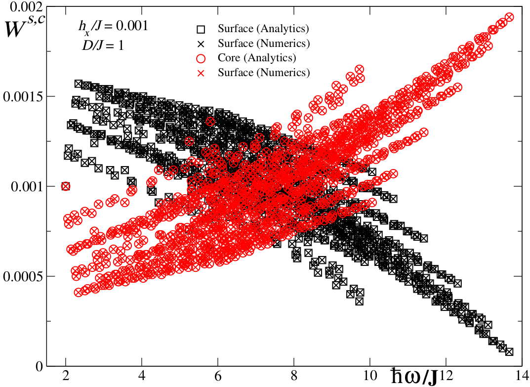
Figure 1: Spectral weight of spin-wave excitations in a box-shaped particle of size $13\times 11\times 7$ and uniform uniaxial anisotropy, in a magnetic field along the $x$ direction.

The procedure to determine the weight of surface and core spins in the energy spectrum has been described in Subsection 2.2.1. In order to compare the spectral weights inferred from the analytical expressions in Eq. (10) et seq to those obtained by the numerical method, we consider a box-shaped particle with a simple cubic lattice. In order to avoid spurious effects that could be due to highly symmetric systems we chose to investigate a particle with sides of different lengths, e.g. $N_{x}=13,\ N_{y}=11,\ N_{z}=7$. In Fig. 1 we present a plot of the spectral weight as a function of the energy $\hbar\omega$ (here $\hbar=1$) in units of the nearest-neighbor exchange coupling $J$, with $J_{c}=J_{cs}=J_{s}=J$. We have considered a static magnetic field along the $x$ axis and a (uniform) uniaxial anisotropy for both the core and surface spins with a common easy axis along the $z$ direction and anisotropy constant $D/J=1$. The large core anisotropy $D=J$ is merely introduced in order to shift the whole spectrum by $2J$ and thereby to highlight the uniform mode. We can see that the numerical results fully agree with the spectral weight inferred from the analytical eigenfunctions in Eq. (10). The full spin-wave spectrum of such many-spin systems is rather complex as it exhibits many branches, and thence does not lend itself to a simple interpretation of the various involved excitations. To that end, we have considered a representative, though much simpler, system that consists of three coupled spin layers for which the excitation spectrum can be computed, with the possibility to disentangle the contributions of the surface and core layers. This is done in B. The major difference is that the three-layer toy model exhibits only three branches and we can see that the surface spins dominate the low-frequency excitations. On the other hand, the various branches of the many-spin system correspond to different modes running in the $k-$space of a simple cubic lattice. For instance, a quick inspection of Fig. 8 shows that the surface is dominant away from the Brillouin zone center. In addition, the effect of the surface exchange coupling ($J_{s}$) has been checked for the same particle without external magnetic field or anisotropy. We have seen that at low excitation energies, the spectral weights of the surface spins are always higher than those of the core spins. However, as $J_{s}$ increases the branches of excitations that preferentially involve surface spins merge with other branches and thus decrease the surface contribution. This effect is more clearly seen in the framework of the toy-model as shown in Fig. 8.

3.2 Absorbed power

3.2.1 Box-shaped nanoparticles

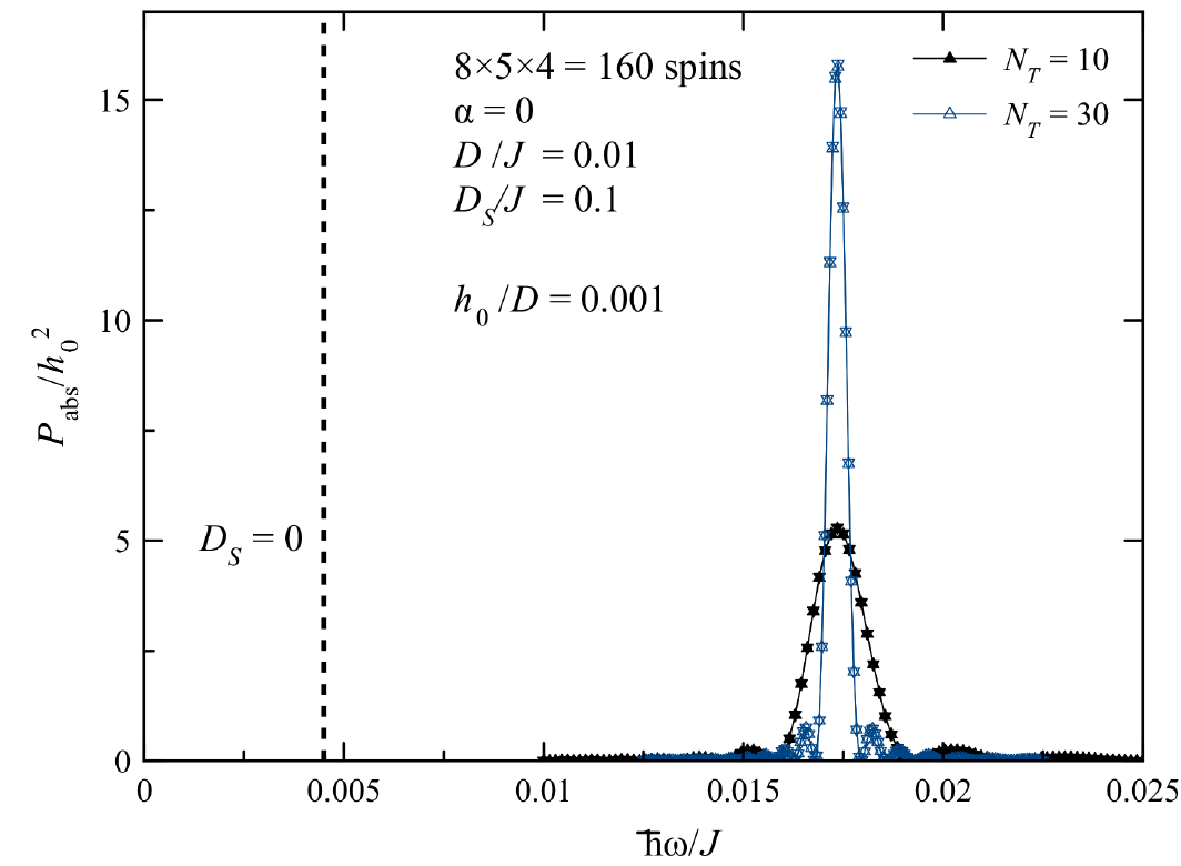
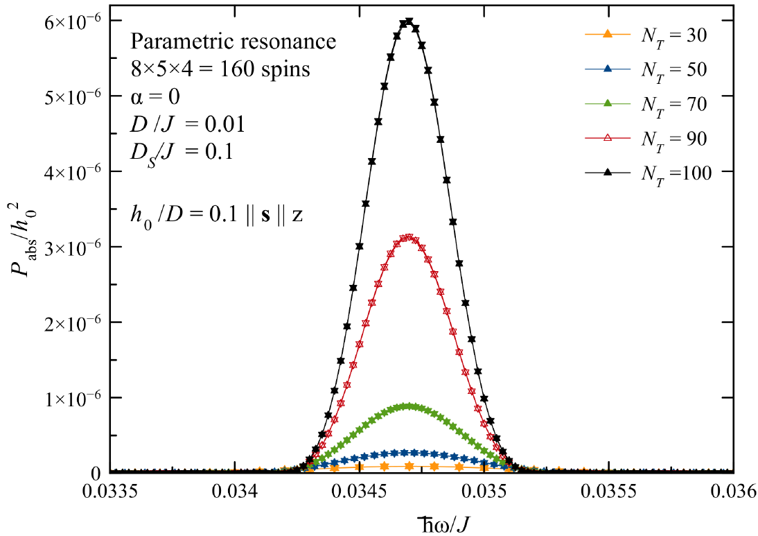
Figure 2: Absorbed power in a $8\times 5\times 4$ cubic particle. Left panel: Magnetic resonance peak at $\hbar\omega/J=0.0174$ for two different pumping times. The vertical dotted line shows the position of the peak for $D_{S}=0$. Right panel: Parametric resonance peak at the double frequency $\hbar\omega/J=0.0347$.

To see how our numerical method of Section 2.2.2 is implemented, we start with a small particle containing $160$ ($=8\times 5\times 4$) spins that is flat in the $xy$ plane, with the anisotropy axis in the $z$ direction and the ac field applied along the $x$ axis (if not stated otherwise). The magnetic-resonance (MR) peak in Fig. 2 (left panel) is seen at $\hbar\omega/J=0.0174$ that is far to the right of the peak position $\hbar\omega/J=0.0045$ obtained for $D_{S}=0$. This can be understood as the result of $xy$ planes having a larger area, their stabilizing action for $D_{S}>0$ is stronger than the destabilizing action of other surfaces, in a qualitative agreement with Eq. (20). One can see that increasing the pumping time from $N_{T}=10$ to $N_{T}=30$ makes the resonance peak narrower and higher, in accord with Eq. (18). Moreover, one can see the zeros of $P_{\mathrm{abs}}$ and small satellite maxima between them. All the numerical work presented below uses $N_{T}=10$, as this is sufficient to find the positions of the resonance maxima. This is a shape effect indicating that the precession of spins is elliptic rather than circular. In such cases parametric resonance can be observed. Thus for the same particle, we also performed a parametric-resonance calculation, directing the ac field in the spin direction $z$. The results showing the initial stages of the exponential parametric instability at the double frequency of the MR peak $\hbar\omega/J=0.0347$ are shown in Fig. 2 (right panel). The parametric-resonance peak has a different structure and its growth accelerates with the pumping time. However, the parametric resonance requires a much stronger amplitude of the ac field and longer pumping times, as compared with MR peaks. In the sequel we will only concentrate on the latter.

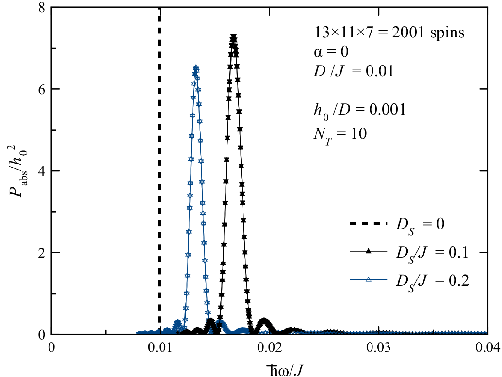
Figure 3: Absorbed power in a $13\times 11\times 7$ cubic particle. Left panel: Low-frequency peak. The vertical dotted line shows the position of the peak for $D_{S}=0$. Right panel: Both low-frequency peaks (far left) and high-frequency peaks.

In order to identify the contributions from the core and surface spins in the absorbed power we have investigated a cluster with a similar aspect ratio as the cluster with $13\times 11\times 7=1001$ spins [see Fig. 3], studied in Fig. 1 and for which the diagonalization method presented in Section 2.2.1 allows for a discrimination between the contributions from the core and surface.

Taking the (space) Fourier transform of the spin $s_{i}(t)$ in Eq. (15) we obtain the power absorbed by the $\bm{k}=\bm{0}$ mode

$$P_{\mathrm{abs}} = -\frac{1}{t_{f}}\intop_{0}^{t_{f}}dt\left(g\mu_{B}\right)\delta\bm{s}_{\bm{k=0}}(t)\cdot\dot{\mathbf{H}}_{\mathrm{ac}}\left(t\right)$$ (21)

$$= -\frac{1}{t_{f}}\intop_{0}^{t_{f}}dt\left(g\mu_{B}\right)\sum_{\alpha=x,y,z}\delta s_{\bm{k=0}}^{\alpha}(t){\bf e}_{\alpha}\cdot\dot{\mathbf{H}}_{\mathrm{ac}}\left(t\right).$$

Then, setting $\bm{k}=\bm{0}$ in Eq. (9)

$$\delta\bm{s}_{\bm{k=0}}\left(t\right) = \delta s_{\bm{k=0}}^{\alpha}\left(0\right)e^{i\hbar\omega_{\bm{k}=\bm{0}}t}=\left(\sum_{j=1}^{\mathcal{N}}\sum_{\alpha=x,y,z}\mathcal{D}_{\bm{k}=\bm{0},j}^{\alpha}\bm{e}_{j}^{\alpha}\right)e^{i\hbar\omega_{\bm{k}=0}t}$$ (22)

we obtain

$$P_{\mathrm{abs}} = -\frac{1}{t_{f}}\intop_{0}^{t_{f}}dte^{i\hbar\omega_{\bm{k}=\bm{0}}t}\left(\sum_{j=1}^{\mathcal{N}}\sum_{\alpha=x,y,z}\mathcal{D}_{\bm{k}=\bm{0},j}^{\alpha}\right)\left(\bm{e}_{j}^{\alpha}\cdot g\mu_{B}\dot{\mathbf{H}}_{\mathrm{ac}}\left(t\right)\right)$$ (23)

Now, since the vectors ${\bf e}_{j}^{\alpha}$ are all parallel to each other, i.e. ${\bf e}_{j}^{\alpha}={\bf e}^{\alpha}$, the equation above simplifies into the following form

$$P_{\mathrm{abs}} = \left[-\frac{1}{t_{f}}\intop_{0}^{t_{f}}dte^{i\hbar\omega_{\bm{k}=\bm{0}}t}\left(g\mu_{B}\right)\left(\sum_{j=1}^{\mathcal{N}}\sum_{\alpha=x,y,z}\mathcal{D}_{\bm{k}=\bm{0},j}^{\alpha}\right)\right]\left(\bm{e}^{\alpha}\cdot\dot{\mathbf{H}}_{\mathrm{ac}}\left(t\right)\right)$$ (24)

which suggests that we can introduce the power absorbed by the degree of freedom (mode) corresponding to the component $\alpha=x,y,z$. Indeed, we can write

$$P_{\mathrm{abs}}^{\alpha} = \left(\sum_{j=1}^{\mathcal{N}}\mathcal{D}_{\bm{k}=\bm{0},j}^{\alpha}\right)\times\left[-\frac{1}{t_{f}}\intop_{0}^{t_{f}}dte^{i\hbar\omega_{\bm{k}=\bm{0}}t}\bm{e}^{\alpha}\cdot g\mu_{B}\dot{\mathbf{H}}_{\mathrm{ac}}\left(t\right)\right].$$ (25)

This in turn can be rewritten as

$$P_{\mathrm{abs}}^{\alpha}\left(\bm{k}=0\right)=C_{\bm{k}=\bm{0}}^{\alpha}\times\widetilde{P}_{\bm{k}=\bm{0}}^{\alpha}$$ (26)

where

$$C_{\bm{k}=\bm{0}}^{\alpha}\equiv\sum_{j=1}^{\mathcal{N}}\mathcal{D}_{\bm{k}=\bm{0},j}^{\alpha}$$ (27)

is the statistical weight of the $\bm{k}=\bm{0}$ mode and

$$\widetilde{P}_{\bm{k}=\bm{0}}^{\alpha}\equiv-\frac{1}{t_{f}}\intop_{0}^{t_{f}}dte^{i\hbar\omega_{\bm{k}=\bm{0}}t}\bm{e}^{\alpha}\cdot g\mu_{B}\dot{\mathbf{H}}_{\mathrm{ac}}\left(t\right).$$ (28)

This means that the absorbed power (per mode) is proportional to the sum of the coefficients of the wave-functions. As such, instead of calculating the absorbed power as defined by Eq. (15) we can calculate and plot the coefficients $C_{\bm{k}=\bm{0}}^{\alpha}$.

For a clearer analysis of the modes appearing in the absorbed power spectrum, we first focus on the case of a box-shaped sample with the same exchange constant everywhere, namely $J_{c}=J_{cs}=J_{s}=J$, and without any anisotropy. All the spins are then identical and the excitation spectrum is given by a single energy band in the $k$-space as in Eq. (10). Hence, each mode can be unequivocally labeled by its wave-vector $\bm{k}$ only. According to the definition of the coefficients $C_{k}^{\alpha}$, the power can only be absorbed when the field couples to the uniform mode, i.e for $C_{\bm{k}=\bm{0}}^{\alpha}=1$. On the other hand, for all other values of the wave-vector $\mathbf{k}$ it can be easily shown that

$$C_{\bm{k}\neq\bm{0}}^{\alpha}=\prod_{\alpha=x,y,z}\frac{\sin\left(N_{\alpha}k_{\alpha}\right)}{\sin\left(\frac{k_{\alpha}}{2}\right)}=0.$$ (29)

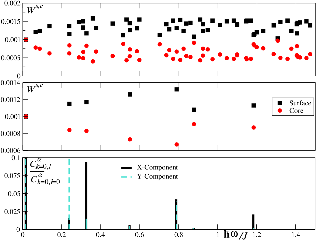
Figure 4: Spectral weight of spin-wave excitations in a box-shaped particle of size $13\times 11\times 7$. Upper panel : spectral weight for the low frequency region. Middle panel: weights for $C_{k=0,\ell}^{\alpha}\neq 0$. The lower panel correspond to the coefficient $C_{k=0,\ell}^{\alpha}$ for the different components of the spins defined in Eq. (26), normalized that of the uniform mode $k=\ell=0.$

In contrast to this simple case, for a system with different types of local environments, as a consequence of an inhomogeneous exchange coupling ($J_{c}\neq J_{cs}\neq J_{s}$), or of different types of on-site anisotropies (surface and core), different energy bands appear in the $\bm{k}$-space. This can be easily understood in the framework of the toy model presented in B and shown in Fig. 8). The analysis of such a situation requires an additional band index ($\ell$) in order to label each mode of energy $\hbar\omega_{k,\ell}$ and coefficients $C_{k,\ell}^{\alpha}$. Consequently, the absorbed power can be attributed to the non-uniform modes at $\bm{k}=\bm{0}$. This is shown in Fig. 4 which presents the spectral weight and the wave-function coefficients $C_{k,\ell}^{\alpha}$ in the low-frequency regime, with a surface anisotropy $D_{S}/J=0.1$. The upper panel shows the weights of the core and surface spins for all low frequency modes. The middle and lower panels respectively present the weights of the power-absorbing modes and the coefficient $C_{k,\ell}^{\alpha}$, normalized by that of the uniform mode ($k=\ell=0$). We can see that the peaks in the absorbed power in Fig. 3 (for $D_{S}/J=0.1$) coincide with the peaks in black in Fig. 4, i.e the peaks obtained for an ac field applied along the $x$ axis. The peaks in black obtained for $\hbar\omega/J=0.24,\ 0.54,\ 0.88$ in Fig. 4 are not seen in Fig. 3 because the intensities of these peaks are too low compared to the satellites obtained from the absorbed power, described in subsection 2.2.3. The first peak $\hbar\omega/J=0.017$ (in Fig. 3) corresponds to the uniform mode. The latter corresponds to an equal contribution (50%) to the spectral weight from the core and surface spins. Indeed, we have checked that this is in agreement with the lowest energy mode shown in Fig. 4 for which the core and surface spectral weights coincide [see middle panel]. Since the contribution of both core and surface spins is at its maximum in this case, the low-energy peak in Fig. 3 and 4 exhibits the highest intensity. The higher-frequency peaks in black correspond to the non-uniform mode ($\bm{k}=0,\ \ell>0$) due to the anisotropy and therefore they occur with a lower intensity. These peaks have a dominant contribution from the surface spins (see Tab. 1).

$\hbar\omega/J$	0.017	0.33	0.79	1.18
Surface (%)	50	60	70	60
Core (%)	50	40	30	40

Table 1: Contributions to the spectral weight from the surface and core spins for the cluster $13\times 11\times 7$ with $D_{S}/J=0.1$ and a time-dependent field applied along the $x$ axis (i. e. Black peaks of Fig.4).

The peaks in cyan in Fig.4 are obtained for a time-dependent field along the $y$ axis. These peaks appear with the same frequencies as the peaks in black but with different intensities. In addition, the contributions from the surface and core spins may vary from one type of peaks to the other.

For the same nanocluster and in accordance with Eq. (20), in Fig. 3 the position of the low-frequency peak shifts to the right as $D_{S}$ increases from zero (compare with the vertical line at $D_{S}=0$). However, a further increase of SA reverses this tendency, as can be seen from the curve $D_{S}/J=0.2$. This mode softening can be attributed to the second-order effect of surface anisotropy. On the other hand, in the high-frequency part of the spectrum one can observe three peaks that could be attributed to three different types of the nanocluster facets with different local environment (or effective fields). Note that the positions of the peaks are nearly the same for $D_{S}/J=0.1$ and $D_{S}/J=0.2$, which hints at the predominant exchange origin of these modes.

3.2.2 Size effect and application to nanocubes

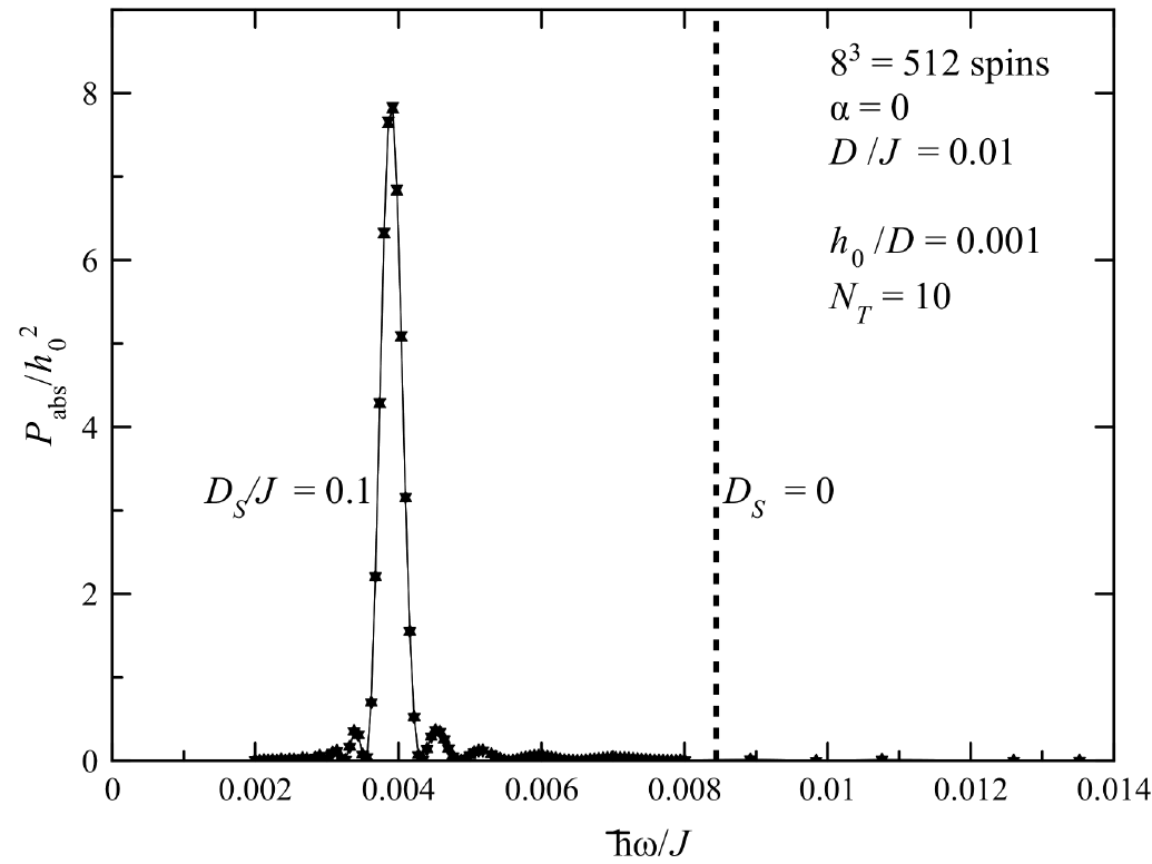
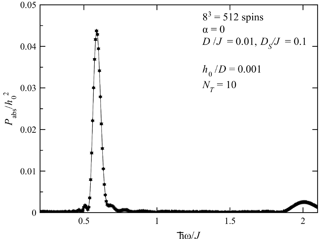
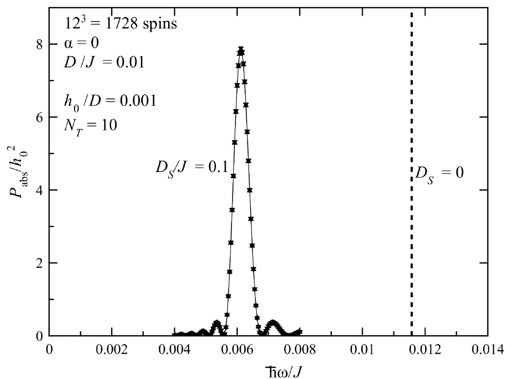
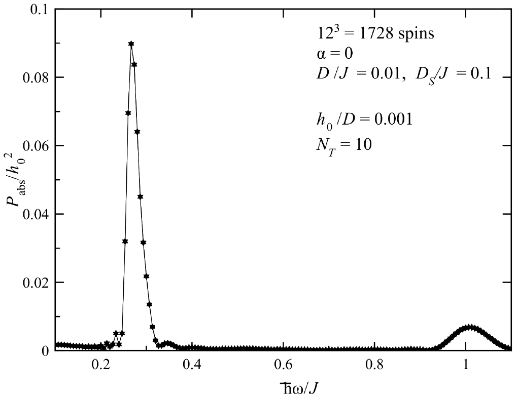
Figure 5: Absorbed power for $8\times 8\times 8$ and $12\times 12\times 12$ particles with a focus on the low-frequency peaks in the left column and the high-frequency peaks in the right column. The vertical dotted line shows the position of the peak for $D_{S}=0$.

The investigation of size effects in general (i.e. without any rotational symmetry) is a rather involved task since upon increasing the size the number of modes increases and their degeneracy makes it difficult to disentangle their contributions to the spectral weight. This is one of the reasons for which we have decided to focus on cubic samples. In fact, today samples of (iron) nanocubes are routinely investigated in experiments since their synthesis has become fairly well controlled.

Accordingly, the results for the absorbed power for the $8\times 8\times 8$ particle (512 spins) are shown in Fig. 5. One can see a strong peak at $\hbar\omega=0.0039J$ that corresponds to nearly coherent precession of all spins in the particle. Because of the second-order effect of SA [30] this peak is shifted to the left from its position for $D_{S}=0$, shown by the vertical dotted line at $\hbar\omega_{0}=2D\mathcal{N}_{\mathrm{core}}/\mathcal{N}=0.0084J$. Note that the first-order formula, Eq. (20), does not capture this effect. Here one cannot use $D_{S}/J=0.2$ because further shift of the peak to the left renders the collinear spin configuration along the $z$ axis unstable.

The lower panel of Fig. 5 shows similar results for a larger particle of $12\times 12\times 12=1728$ spins. Here the low-frequency peak is shifted to the right in comparison with the $8\times 8\times 8$ particle, and which can be explained by the smaller fraction of surface spins. The leftmost and strongest of high-frequency peaks here is larger and shifted to the left. Note that for both of these sizes high-frequency peaks are much smaller than the main low-frequency peak (notice the difference in scale between the left and right panels). By way of illustration, we consider an Fe nanocube of side $a=8\,\mathrm{nm}$ [18, 5, 6, 31, 12, 32]. This corresponds to a nanocluster of size $27\times 27\times 27$ particle whose absorption spectrum is shown in Fig. 6.

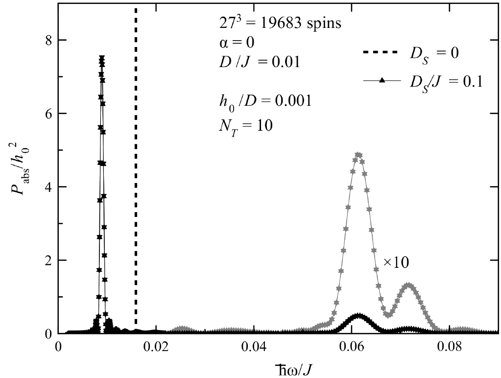
Figure 6: Same as in Fig. 5 but for the cluster $27\times 27\times 27$.

Although the present paper is focused on theoretical aspects, a few predictions can be made for realistic iron nanocubes studied today in many experiments. Both synthesis and recent experimental developments have provided systems with optimized structures that could be mimicked by the simplified model studied here. In particular, using some oxygen and plasma treatment it seems that the ligands and oxide shell could be effectively removed, leaving us with ferromagnetic nanocubes, see e.g. Ref. [18]. Would FMR measurements on such nanocubes become possible, the observed spectrum should exhibit the features described in the present work, e.g. a low-energy peak at around $10{\rm\ GHz}$ for the uniform mode, followed by higher-energy excitations that couple to the latter. In addition, the aspect-ratio of box-shaped (non-cubic) samples can be figured out by this technique upon checking whether a parametric resonance feature appears in the spectrum. In regards with the values of the physical parameters taken in our calculations, we note that the ratio of the magneto-crystalline anisotropy to the exchange coupling ($D/J$) is here taken at least an order of magnitude larger than in typical iron systems. The reason is that lower values of this ratio require much more time-consuming calculations while the physical picture remains the same. More precisely, the calculation for typical iron materials with $D/J\sim 10^{-3}$ would lead to a down-shift of the low-frequency peak roughly by a factor of 10 while the high-frequency peaks should practically remain the same.

As compared with the sizes dealt with above, here the high-frequency peak is even larger and even more shifted to the left, so that the low- and high-frequency spectra can be plotted on the same graph. In addition, the high-frequency peak resolves into two peaks. The main high-frequency peak, shown in the right column of Fig. 5, can be interpreted as being due to the precession of the spins located near the facets of the cube. Since this precession mode is non-uniform (it has a non-zero $k=0$ component) there is exchange energy involved and this is why the precession frequency is high. With an increasing size, the exchange energy per spin in this mode decreases, and so does its frequency. The splitting of the main high-frequency peak seen for the $27\times 27\times 27$ particle can be explained by the fact that SA induces an increase of the mode stiffness at the two $xy$ planes (the small peak on the right) and to a decrease of the mode stiffness at the four other surfaces (the big peak on the left).

4 Conclusion

Through a systematic numerical investigation, backed by analytical calculations for special cases, we have studied and distinguished the role of surface and core spins in box-shaped magnetic nanoparticles. We have focused this work on this specific shape inspired by numerous experimental studies of iron nanocubes which are now available in well controlled cubic shapes and sizes. On the other hand, ferromagnetic resonance measurements on “isolated” nanoelements has now become possible with the necessary sensitivity for measuring the absorbed power.

Accordingly, we have computed the absorbed power as a function of the excitation frequency and have shown that it is possible to attribute the different contributions of the surface and those of the core spins to the various peaks obtained in our calculations. In particular, the low-energy peak, corresponding to the $\bm{k=0}$ mode, consists of equal contributions from the surface and core spins. Furthermore, in the case of less symmetric box-shaped samples with Néel surface anisotropy, we observe an elliptic precession of the spins whose signature can be seen in a parametric resonance experiment, where a small signal should be detected at twice the frequency of the standard magnetic resonance response.

Appendix A Energy Hessian in spherical coordinates

At each site $i$ of the cluster’s lattice we may define the reference system with the spherical coordinate $(\theta_{i},\varphi_{i})$ and basis basis $(\mathbf{s}_{i},\mathbf{e}_{\theta_{i}},\mathbf{e}_{\varphi_{i}})$ related to the Cartesian coordinates by

$$\mathbf{s}_{i} = \mathbf{e}_{\varphi_{i}}\left(\begin{array}[]{c}\sin\theta_{i}\cos\varphi_{i}\\ \sin\theta_{i}\sin\varphi_{i}\\ \cos\theta_{i}\end{array}\right),\ \mathbf{e}_{\theta_{i}}=\left(\begin{array}[]{c}\cos\theta_{i}\cos\varphi_{i}\\ \cos\theta_{i}\sin\varphi_{i}\\ -\sin\theta_{i}\end{array}\right),\ \mathbf{e}_{\varphi_{i}}=\left(\begin{array}[]{c}-\sin\varphi_{i}\\ \cos\varphi_{i}\\ 0\end{array}\right).$$ (39)

From this we derive

$$\partial_{\theta_{i}}\mathbf{s}_{i} = \mathbf{e}_{\theta_{i}},\quad\partial_{\varphi_{i}}\mathbf{s}_{i}\mathbf{=}\sin\theta_{i}\,\mathbf{e}_{\varphi_{i}},$$

$$\partial_{\theta_{i}}\mathbf{e}_{\theta_{i}} = -\mathbf{s}_{i}\mathbf{,\quad}\partial_{\varphi_{i}}\mathbf{e}_{\theta_{i}}=\cos\theta_{i}\,\mathbf{e}_{\varphi_{i}},$$

$$\partial_{\theta_{i}}\mathbf{e}_{\varphi_{i}} = 0,\;\partial_{\varphi_{i}}\mathbf{e}_{\varphi_{i}}=-\left(\sin\theta_{i}\,\mathbf{s}_{i}+\cos\theta_{i}\,\mathbf{e}_{\theta_{i}}\right).$$

leading to $\delta\mathbf{s}_{i}=\delta\theta_{i}\partial_{\theta_{i}}\mathbf{s}_{i}\mathbf{+}\delta\varphi_{i}\partial_{\varphi_{i}}\mathbf{s}_{i}\mathbf{=}\delta\theta_{i}\mathbf{e}_{\theta_{i}}\mathbf{+}\delta\varphi_{i}\sin\theta_{i}\,\mathbf{e}_{\varphi_{i}}$. Then using the gradient

$$\partial_{\mathbf{s}_{i}}\equiv\mathbf{\bm{\nabla}}_{i}=\mathbf{e}_{\theta_{i}}\partial_{\theta_{i}}+\mathbf{e}_{\varphi_{i}}\frac{1}{\sin\theta_{i}}\,\partial_{\varphi_{i}}\mathbf{,}$$ (40)

we get $\delta\mathbf{s}_{i}\mathbf{\cdot\bm{\nabla}}_{i}=\delta\theta_{i}\,\partial_{\theta_{i}}+\delta\varphi_{i}\,\partial_{\varphi_{i}}$. This implies for an arbitrary function $f(\theta_{i}\varphi_{i})$

$$\partial_{\theta_{i}}f=\mathbf{e}_{\theta_{i}}\cdot\mathbf{\bm{\nabla}}_{i}f,\quad\partial_{\varphi_{i}}f=\sin\theta_{i}\,\mathbf{e}_{\varphi_{i}}\cdot\mathbf{\bm{\nabla}}_{i}f.$$ (41)

Since the spin deviation $\delta\bm{s}_{k}$ can be written in terms of $\delta\theta_{k}$ and $\delta\varphi_{k}$ Eq. (7) can be written in the basis $\left\{\left({\bf e}_{\theta_{i}},{\bf e}_{\varphi_{i}}\right)\right\}_{i=1,\cdots,\mathcal{N}}=\left\{\bm{\xi}_{\mu}\right\}_{\mu=1,\cdots,2\mathcal{N}}$. Note, however, that in the general case these unit vectors are not orthogonal to each other i.e. $\bm{\xi}_{\mu}\cdot\bm{\xi}_{\nu}\neq\delta_{\mu,\nu}$. In fact, $\delta\bm{s}_{k}$ represents the usual spin-wave deviations from the local equilibrium state of spin ${\bf s}_{k}$, which is denoted by ${\bf s}_{k}^{\left(0\right)}$. The latter represents the quantization direction for the local algebra. It’s well known that $\delta{\bf s}_{k}$ can be written in terms of the spin operators $S_{k}^{\pm}$ which form a local SU(2) algebra with the usual commutation rules, i. e. $\left[S_{i}^{\alpha},S_{j}^{\beta}\right]=i\varepsilon^{\alpha\beta\gamma}\delta_{ij}S_{i}^{\gamma}$, with $\varepsilon^{\alpha\beta\gamma}$ being the Levi-Civita tensor. In particular, spins operating on different sites commute with each other. This implies that the vectors $\delta{\bf s}_{k}$, or more precisely, the transverse vectors $\left\{\left({\bf e}_{\theta_{i}},{\bf e}_{\varphi_{i}}\right)\right\}_{i=1,\cdots,\mathcal{N}}=\left\{\bm{\xi}_{\mu}\right\}_{\mu=1,\cdots,2\mathcal{N}}$ can be represented by the vectors of the orthonormal canonical basis $\left\{\left({\bf e}_{i}\right)\right\}_{i=1,\cdots,\mathcal{N}}$ with $e_{i}^{\alpha}=\delta_{i,\alpha}$.

Assuming that the energy $\mathcal{E}=\sum_{i=1}^{\mathcal{N}}\mathcal{E}_{i},$ is given by a general Hamiltonian we obtain the second derivatives of $\mathcal{E}_{i}$ in terms of its derivative with respect to $\mathbf{s}_{i}$.

$$\bm{\widetilde{\mathcal{H}}}_{ik}(\mathcal{E}_{i})\equiv\left(\begin{array}[]{ll}\partial_{\theta_{i}\theta_{k}}^{2}\mathcal{E}&\frac{1}{\sin\theta_{i}}\partial_{\theta_{k}\varphi_{i}}^{2}\mathcal{E}\\ \\ \frac{1}{\sin\theta_{k}}\partial_{\varphi_{k}\theta_{i}}^{2}\mathcal{E}&\frac{1}{\sin\theta_{i}\sin\theta_{k}}\partial_{\varphi_{k}\varphi_{i}}^{2}\mathcal{E}\end{array}\right).$$ (42)

This is the (pseudo-) Hessian of $\mathcal{E}$ resulting from the action of the (pseudo-) Hessian operator

$$\bm{\widetilde{\mathcal{H}}}_{ik}=\mathbf{\bm{\nabla}}_{k}^{T}\mathbf{\bm{\nabla}}_{i}=\left(\begin{array}[]{cc}\partial_{\theta_{k}}&\frac{1}{\sin\theta_{k}}\partial_{\varphi_{k}}\end{array}\right)\left(\begin{array}[]{c}\partial_{\theta_{i}}\\ \\ \frac{1}{\sin\theta_{i}}\partial_{\varphi_{i}}\end{array}\right).$$ (43)

For a given nanocluster of given size, shape, anisotropy model and the applied field, one first determines the equilibrium state, denoted by $\left\{{\bf s}_{i}^{(0)}=(\theta_{i}^{(0)},\varphi_{i}^{(0)})\right\}_{i=1,\cdots,\mathcal{N}}$, where $\theta_{i}$ and $\varphi_{i}$ are the standard spherical angles defined with respect to the local basis $\left({\bf s}_{i},\mathbf{e}_{\theta_{i}},\mathbf{e}_{\varphi_{i}}\right)$ at site $i$.

The effective field is defined by $\mathbf{H}_{\mathrm{eff},i}=-\delta_{\mathbf{s}_{i}}\mathcal{E}=-\mathbf{\bm{\nabla}}_{i}\mathcal{E}$, such that the four second derivatives read

$$\partial_{\theta_{i}\theta_{k}}^{2}\mathcal{E} = \delta_{ik}\left[\mathbf{s}_{i}\cdot-\mathbf{e}_{\theta_{i}}\cdot\left(\mathbf{e}_{\theta_{i}}\cdot\mathbf{\bm{\nabla}}_{i}\right)\right]\mathbf{H}_{\mathrm{eff},i}-\left(1-\delta_{ik}\right)\mathbf{e}_{\theta_{i}}\cdot\left[\mathbf{e}_{\theta_{k}}\cdot\mathbf{\bm{\nabla}}_{k}\right]{\bf H}_{\mathrm{eff},i},$$

$$\partial_{\varphi_{k}\varphi_{i}}^{2}\mathcal{E} = \delta_{ik}\sin\theta_{i}\left[\left(\sin\theta_{i}\,\mathbf{s}_{i}+\cos\theta_{i}\,\mathbf{e}_{\theta_{i}}\right)-\sin\theta_{i}\,\mathbf{e}_{\varphi_{i}}\cdot\left(\mathbf{e}_{\varphi_{i}}\cdot\mathbf{\bm{\nabla}}_{i}\right)\right]\mathbf{H}_{\mathrm{eff},i}$$

$$-\left(1-\delta_{ik}\right)\sin\theta_{i}\sin\theta_{k}\,\mathbf{e}_{\varphi_{i}}\cdot\left[\mathbf{e}_{\varphi_{k}}\cdot\mathbf{\bm{\nabla}}_{k}\right]\mathbf{H}_{\mathrm{eff},i},$$

$$\partial_{\theta_{k}\varphi_{i}}^{2}\mathcal{E} = -\delta_{ik}\left[\cos\theta_{i}\,\mathbf{e}_{\varphi_{i}}\cdot+\sin\theta_{i}\,\mathbf{e}_{\varphi_{i}}\cdot\left(\mathbf{e}_{\theta_{i}}\cdot\mathbf{\bm{\nabla}}_{i}\right)\right]\mathbf{H}_{\mathrm{eff},i}$$

$$-\left(1-\delta_{ik}\right)\sin\theta_{i}\,\mathbf{e}_{\varphi_{i}}\cdot\left[\mathbf{e}_{\theta_{k}}\cdot\mathbf{\bm{\nabla}}_{k}\right]\mathbf{H}_{\mathrm{eff},i},$$

$$\partial_{\varphi_{k}\theta_{i}}^{2}\mathcal{E} = -\delta_{ik}\left[\cos\theta_{i}\,\mathbf{e}_{\varphi_{i}}\cdot+\sin\theta_{i}\,\mathbf{e}_{\theta_{i}}\cdot\left(\mathbf{e}_{\varphi_{i}}\cdot\mathbf{\bm{\nabla}}_{i}\right)\right]\mathbf{H}_{\mathrm{eff},i}$$ (44)

$$-\left(1-\delta_{ik}\right)\sin\theta_{k}\,\mathbf{e}_{\theta_{i}}\cdot\left(\mathbf{e}_{\varphi_{k}}\cdot\mathbf{\bm{\nabla}}_{k}\right)\mathbf{H}_{\mathrm{eff},i}.$$

It is understood that all these derivatives and the pseudo-Hessian have to be evaluated at the equilibrium state $\left\{{\bf s}_{i}^{(0)}=(\theta_{i}^{(0)},\varphi_{i}^{(0)})\right\}_{i=1,\cdots,\mathcal{N}}$.

Appendix B Toy model

In order to achieve a simple physical picture of the contributions of core and surface spins to the spectral weight, together with a possible comparison with the numerical method developed in Subsection 2.2.1, we have built a toy model that captures the main feature we want to illustrate but which is analytically tractable. Accordingly, we consider a ferromagnet composed of 3 coupled layers as sketched in Fig. 7. Each layer is assumed to be infinite in $x$ and $y$ directions.

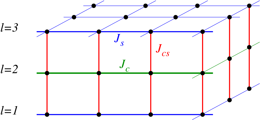
Figure 7: $2D$ Slab of $3$ atomic layers with exchange couplings $J_{s}$ (surface), $J_{cs}$ (core-surface) and $J_{c}$ (core).

The spin Hamiltonian of such a system is the Heisenberg model

$$\begin{array}[]{lll}\mathcal{H}&=&-{\displaystyle\sum_{l=1,3}}J_{l}{\displaystyle\sum_{i}}\bm{S}_{i,l}\cdot\left(\bm{S}_{i+x,l}+\bm{S}_{i+y,l}\right)-J_{cs}{\displaystyle\sum_{i}}\bm{S}_{i,2}\cdot\left(\bm{S}_{i,1}+\bm{S}_{i,3}\right)\end{array},$$ (45)

where $\bm{S}_{i,l}$ is the spin at site $i$ within the layer $l$, and $J_{l=1,3}\equiv J_{s}$ and $J_{2}\equiv J_{c}$. We restrict ourselves to the case of a ferromagnet with $J_{l}>0,J_{cs}>0$. In the spin-wave approach we choose $z$ as the quantization axis and perform a Holstein-Primakoff transformation

$$S_{i,l}^{z} = S_{i,l}^{-}S-a_{i,l}^{\dagger}a_{i,l},\qquad S_{i,l}^{+}\simeq\sqrt{2S}a_{i,l},\qquad S_{i,l}^{-}\simeq\sqrt{2S}a_{i,l}^{\dagger}.$$ (46)

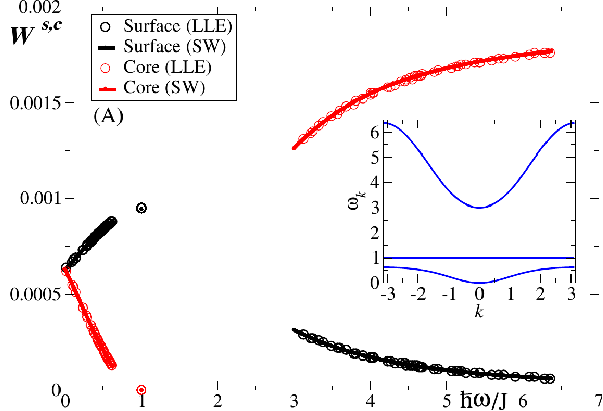
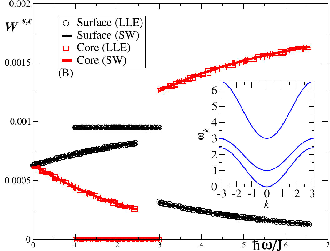
Figure 8: Surface and core spectral weights against the magnon energy for $j_{c}=j_{cs}=1$ and with $j_{s}=0\ (A),\ j_{s}=0.5\ (B)$.

Then, we rewrite the Hamiltonian (45) in terms of the real-space magnon operators $a_{i,l}$ and $a_{i,l}^{\dagger}$. The resulting expression can be partially diagonalized after a Fourier transformation with respect to the $\left(x,y\right)$ directions

$$\begin{array}[]{lll}\frac{\mathcal{H}}{S}&=&{\displaystyle\sum_{q_{x},q_{y}}}\left(a_{q,1}^{\dagger}\ a_{q,2}^{\dagger}\ a_{q,3}^{\dagger}\right)\mathcal{J}\left(\bm{q}\right)\cdot\left(\begin{array}[]{c}a_{q,1}\\ a_{q,2}\\ a_{q,3}\end{array}\right)+{\rm C^{te}},\end{array}$$ (47)

where $\mathcal{J}\left(\bm{q}\right)$ is the coupling matrix

$$\mathcal{J}\left(\bm{q}\right)=\left(\begin{array}[]{ccccc}\mathcal{J}_{11}&&-J_{cs}&&0\\ -J_{cs}&&\mathcal{J}_{22}&&-J_{cs}\\ 0&&-J_{cs}&&\mathcal{J}_{33}\end{array}\right),$$ (48)

with $\mathcal{J}_{11}=\mathcal{J}_{33}=2J_{s}\left(1-\gamma_{\bm{q}}\right)+J_{cs}$ and $\mathcal{J}_{22}=2J_{c}\left(1-\gamma_{\bm{q}}\right)+2J_{cs}$, and $\gamma_{\bm{q}}\equiv\frac{1}{2}\left(\cos q_{x}+\cos q_{y}\right)$. We use $J_{c}$ as our energy scale and define the reduced couplings $j_{cs}\equiv J_{cs}/J_{c}$ and $j_{s}\equiv J_{s}/J_{c}$. The three dispersions are then given by

$$\begin{array}[]{lll}\omega_{\pm}\left(j_{cs},j_{s},\bm{q}\right)&=&\frac{3}{2}j_{cs}+\left(1+j_{s}\right)\left(1-\gamma_{\bm{q}}\right)\\ \\ &&\pm\frac{1}{2}\left\{\left[3j_{cs}+2\left(1+j_{s}\right)\left(1-\gamma_{\bm{q}}\right)\right]^{2}\right.\\ &&\left.\qquad-8\left(1-\gamma_{\bm{q}}\right)\left[j_{cs}\left(1+j_{s}\right)+2j_{s}\left(1-\gamma_{\bm{q}}\right)\right]\right\}^{1/2}\\ \\ \omega_{0}\left(j_{cs},j_{s},\bm{q}\right)&=&j_{cs}+2j_{s}\left(1-\gamma_{\bm{q}}\right).\end{array}$$ (49)

The spectral weights are then obtained as the squares of the projections of the eigenvectors onto the canonical basis $e_{i}^{\alpha}=\delta_{i}^{\alpha},i=1,2,3;\alpha=x,y,z$. These weights depend on the physical parameters such as the exchange couplings and anisotropy constants. Upon summing over the wave vectors $\bm{q}$ within the first Brillouin zone, one can plot the spectral weights as functions of $\omega\left(\bm{q}\right)$.

In Fig. 8 we present the spectral weight of the surface and core spins as a function of the magnon energy for the three energy bands, along the path $q_{x}=q_{y}$, corresponding to the three dispersions (49). The circles and squares are the results for a finite cluster ($N_{x}=N_{y}=23$) dealt with using the numerical method of Subsection 2.2.1, with periodic boundary conditions in the $x$ and $y$ directions. The full lines are the results obtained within the spin-wave approach presented above. The results in Fig. 8 exhibit a very good agreement between the numerical and analytical approaches for all values of the exchange parameters.

In the spin-wave calculation we consider blocks of three spins, belonging to layers 1, 2, 3. These blocks are coupled to one another by lateral (in-plane) couplings. The spin-wave dispersion, as shown in the inset of Fig. 8, has three branches: the lowest branch corresponds to the ferromagnetic magnon excitations with the 3 spins precessing in phase. By computing the spectral weight associated with this branch, one finds that the surface contribution dominates (apart from the uniform mode at $\bm{k}=0$) because the corresponding modes require less energy to be excited. In contrast, the high-energy branch corresponds to the situation where the end spins (layers) precess with opposite phases. The spectral weight is then dominated by the core owing to a higher spin stiffness. For the particular case of $j_{s}=0$, the magnon dispersion exhibits a non-dispersive branch at $\omega_{k}=1$ [see inset of Fig. 8 (left)]. This intermediate branch follows from the fact that the bottom and top layer spins are not coupled within their respective planes. Therefore, creating an excitation within the top or bottom layer is costless, leading to a mode with constant energy in $k$-space. Obviously, this branch corresponds to excitations that are localized at the surface. This can be seen by examining the spectral weight for which the core contribution vanishes.

As the surface exchange coupling increases (i.e. $j_{s}>0$) more dispersion is observed and the branches start to merge for some magnon energies. Hence, the spectral weight changes both qualitatively and quantitatively: the gaps close and the surface and core contributions become more and more entangled.

The calculation of the absorbed power for this system yields one absorption peak for the uniform mode corresponding to the lower energy band in Fig.8. The eigenfunctions for the three energy bands at $\bm{k=0}$ are given by

$$\left\{\begin{array}[]{lll}\Psi_{1}&=&\frac{1}{\sqrt{3}}\left(\phi_{S1}+\phi_{C}+\phi_{S2}\right),\\ \Psi_{2}&=&\frac{1}{\sqrt{2}}\left(\phi_{S1}-\phi_{S2}\right),\\ \Psi_{3}&=&\frac{1}{\sqrt{6}}\left(\phi_{S1}-2\phi_{C}+\phi_{S2}\right).\end{array}\right.$$ (50)

Here $\phi_{S1,2}$ corresponds to the surface spins and $\phi_{C}$ to the core spin. The coefficients $C_{k,\ell}$ of these vectors do not vanish (and are all equal) for the vector $\Psi_{1}$ that corresponds to the uniform mode. In order to obtain more absorption peaks in the absorbed power we can introduce a core anisotropy $k_{c}$ but no surface anisotropy. In this case the eigenfunctions corresponding to $\bm{k=0}$ are

$$\left\{\begin{array}[]{lll}\Psi_{1}&=&\frac{2}{N_{1}}\left[\phi_{S1}-\left(1+k_{c}-\sqrt{9+2k_{c}+k_{c}^{2}}\right)\phi_{C}+\phi_{S2}\right],\\ \Psi_{2}&=&\frac{1}{\sqrt{2}}\left(\phi_{S1}-\phi_{S2}\right),\\ \Psi_{3}&=&\frac{2}{N_{3}}\left[\phi_{S1}-\left(1+k_{c}+\sqrt{9+2k_{c}+k_{c}^{2}}\right)\phi_{C}+\phi_{S2}\right],\end{array}\right.$$ (51)

where $N_{1}$ and $N_{3}$ are normalization factors of the wave-vectors $\Psi_{1}$ and $\Psi_{3}$ respectively. We can see that the modes corresponding to $\Psi_{1}$ and $\Psi_{3}$ can contribute to the absorbed power.

References

- [1] Sun S, Murray C B, Weller D, Folks L and Moser A 2000 Science 287 1989–1992 (Preprint http://www.sciencemag.org/content/287/5460/1989.full.pdf) URL http://www.sciencemag.org/content/287/5460/1989.abstract
- [2] Lisiecki I, Albouy P A and Pileni M P 2003 Advanced Materials 15 712–716 ISSN 1521-4095 URL http://dx.doi.org/10.1002/adma.200304417
- [3] Tartaj P, del Puerto Morales M, Veintemillas-Verdaguer S, González-Carreño T and Serna C J 2003 Journal of Physics D Applied Physics 36 182 URL http://stacks.iop.org/0022-3727/36/i=13/a=202
- [4] Lisiecki I and Nakamae S 2014 Journal of Physics Conference Series 521 012007 URL http://stacks.iop.org/0022-3727/41/i=13/a=134011
- [5] Snoeck E, Gatel C, Lacroix L M, Blon T, Lachaize S, Carrey J, Respaud M and Chaudret B 2008 Nano Letters 8 4293–4298 URL http://dx.doi.org/10.1021/nl801998x
- [6] Mehdaoui B, Meffre A, Lacroix L M, Carrey J, Lachaize S, Gougeon M, Respaud M and Chaudret B 2010 Journal of Magnetism and Magnetic Materials 322 L49–L52 (Preprint 0907.4063) URL http://www.sciencedirect.com/science/article/pii/S0304885310003057
- [7] Vonsovskii S V 1966 Ferromagnetic Resonance: The Phenomenon of Resonant Absorption of a High-Frequency Magnetic Field in Ferromagnetic Substances (Pergamon Press, Oxford)
- [8] AG Gurevich and GA Melkov 1996 Magnetization oscillations and waves (Florida: CSC Press)
- [9] B Heinrich 1994 Ferromagnetic resonance in ultrathin film structures Ultrathin magnetic structures II ed Heinrich B and Bland J (Berlin: Springer-Verlag) p 195
- [10] Tran M 2006 Structural and Magnetic properties of colloidal Fe-Pt and Fe cubic nanoparticles Master’s thesis Institut National des Sciences Appliquees de Toulouse Toulouse
- [11] Lee I, Obukhov Y, Hauser A J, Yang F Y, Pelekhov D V and Hammel P C 2011 Journal of Applied Physics 109 07D313 URL http://scitation.aip.org/content/aip/journal/jap/109/7/10.1063/1.3536821
- [12] Kronast F, Friedenberger N, Ollefs K, Gliga S, Tati-Bismaths L, Thies R, Ney A, Weber R, Hassel C, Römer F M, Trunova A V, Wirtz C, Hertel R, Dürr H A and Farle M 2011 Nano Letters 11 1710–1715 pMID: 21391653 (Preprint http://dx.doi.org/10.1021/nl200242c) URL http://dx.doi.org/10.1021/nl200242c
- [13] Gonçalves A M, Barsukov I, Chen Y J, Yang L, Katine J A and Krivorotov I N 2013 Applied Physics Letters 103 172406 (Preprint 1310.7996) URL {http://scitation.aip.org/content/aip/journal/apl/103/17/10.1063/1.4826927}
- [14] Schoeppner C, Wagner K, Stienen S, Meckenstock R, Farle M, Narkowicz R, Suter D and Lindner J 2014 Journal of Applied Physics 116 033913 URL http://scitation.aip.org/content/aip/journal/jap/116/3/10.1063/1.4890515
- [15] Ollefs K, Meckenstock R, Spoddig D, Römer F M, Hassel C, Schöppner C, Ney V, Farle M and Ney A 2015 Journal of Applied Physics 117 223906 URL http://scitation.aip.org/content/aip/journal/jap/117/22/10.1063/1.4922248
- [16] Sidles J A, Garbini J L, Bruland K J, Rugar D, Züger O, Hoen S and Yannoni C S 1995 Rev. Mod. Phys. 67(1) 249–265 URL http://link.aps.org/doi/10.1103/RevModPhys.67.249
- [17] Lavenant H, Naletov V V, Klein O, De Loubens G, Laura C and De Teresa J M 2014 Nanofabrication 1(1) 2299–680X (Preprint 1404.0492)
- [18] Trunova A V, Meckenstock R, Barsukov I, Hassel C, Margeat O, Spasova M, Lindner J and Farle M 2008 Journal of Applied Physics 104 093904 URL http://scitation.aip.org/content/aip/journal/jap/104/9/10.1063/1.3005985
- [19] Sukhova A, Usadel K D and Nowak U 2008 Journal of Magnetism and Magnetic Materials 320 31–35 URL http://www.sciencedirect.com/science/article/pii/S0304885307006580
- [20] Briático J, Maurice J L, Carrey J, Imhoff D, Petroff F and Vaurès A 1999 The European Physical Journal D - Atomic, Molecular, Optical and Plasma Physics 9 517–521 ISSN 1434-6079 URL http://dx.doi.org/10.1007/s100530050491
- [21] Ling T, Xie L, Zhu J, Yu H, Ye H, Yu R, Cheng Z, Liu L, Liu L, Yang G, Cheng Z, Wang Y and Ma X 2009 Nano Letters 9 1572–1576 (Preprint http://dx.doi.org/10.1021/nl8037294) URL http://dx.doi.org/10.1021/nl8037294
- [22] Lacroix L M, Huls N F, Ho D, Sun X, Cheng K and Sun S 2011 Nano Letters 11 1641–1645 pMID: 21417366 (Preprint http://dx.doi.org/10.1021/nl200110t) URL http://dx.doi.org/10.1021/nl200110t
- [23] Kachkachi H and Garanin D A 2001 Physica A Statistical Mechanics and its Applications 300 487–504 (Preprint cond-mat/0001278)
- [24] Kachkachi H and Garanin D A 2001 European Physical Journal B 22 291–300 (Preprint cond-mat/0012017) URL http://dx.doi.org/10.1007/s100510170106
- [25] Krech M, Bunker A and Landau D P 1998 Computer Physics Communications 111 1–13 (Preprint cond-mat/9805214)
- [26] Steinigeweg R and Schmidt H J 2006 Computer Physics Communications 174 853–861 (Preprint cond-mat/0507262)
- [27] Grimsditch M, Leaf G K, Kaper H G, Karpeev D A and Camley R E 2004 Phys. Rev. B 69(17) 174428 URL http://link.aps.org/doi/10.1103/PhysRevB.69.174428
- [28] Grimsditch M, Giovannini L, Montoncello F, Nizzoli F, Leaf G K and Kaper H G 2004 Phys. Rev. B 70(5) 054409 URL http://link.aps.org/doi/10.1103/PhysRevB.70.054409
- [29] Usadel K D 2006 Phys. Rev. B 73(21) 212405 URL http://link.aps.org/doi/10.1103/PhysRevB.73.212405
- [30] Garanin D A and Kachkachi H 2003 Phys. Rev. Lett. 90(6) 065504 URL http://link.aps.org/doi/10.1103/PhysRevLett.90.065504
- [31] Jiang F, Wang C, Fu Y and Liu R 2010 Journal of Alloys and Compounds 503 L31 – L33 ISSN 0925-8388
- [32] O’Kelly C, Jung S J, Bell A P and Boland J J 2012 Nanotechnology 23 435604 URL http://stacks.iop.org/0957-4484/23/i=43/a=435604