1 Introduction

Small magnetic particles have been of much interest owing to their technological applications, mainly in the area of information storage. From the experimental and theoretical point of view, these systems are very interesting for they show superparamagnetism at high temperature and exponentially slow relaxation rates at low temperature due to anisotropy barriers. Although in most of theoretical approaches to the dynamics of a small magnetic particle the latter is considered as a single magnetic moment, deviations from this simple picture become crucial with the reduction of the system size. In magnetic nanoparticles (see, for a review, Ref. [1]), the contribution of the surface to the thermodynamic properties becomes comparable with the bulk contribution, and the magnetisation and other characteristics may be spatially inhomogeneous. The latter is realised due to additional thermal disordering near the surface at elevated temperatures or due to the breaking of symmetry of the crystal field for surface spins, which may result in a strong surface anisotropy. Another manifestation of the symmetry breaking at the surface is the possible unquenching of the orbital moments of surface spins, which may be responsible for a significant increase of the particle’s magnetic moment, e.g. in 3$d$ elements [2].

A finite-size magnetic system with realistic free boundary conditions presents a spatially inhomogeneous many-body problem. A great deal of work up to date has been based on the Monte Carlo (MC) technique for the Ising model. MC technique was also used with the more adequate classical Heisenberg model to simulate idealised isotropic nanoparticles with simple cubic (sc) structure and spherical shape in Ref. [3]. Magnetic nanoparticles with realistic lattice structure were simulated in Ref. [4] taking into account surface anisotropy and dipole-dipole interaction.

Familiar analytical methods such as the mean-field approximation (MFA) and spin-wave theory (SWT) are (at least in their standard form) inapproriate for finite magnetic systems because of the Goldstone mode corresponding to the global rotation of the magnetic moment in zero field. A more sophysticated way to analytically treat finite magnets is to take the limit $D\to\infty$ for the model of $D$-component classical spin vectors, which was introduced by Stanley [5]. Stanley has shown [6] that for $D\to\infty$ the partition function for this model in the bulk coincides with that of the exactly solvable spherical model (SM) [7]. Both models provide a reasonably good approximation (about 5% overall accuracy) to the isotropic classical Heisenberg model in three dimensions. For spatially inhomogeneous systems such as magnetic particles or films with free boundary conditions, these two models become nonequivalent, the SM having been shown to yield unphysical results because of the inappropriate global spin constraint [8]. This drawback was fixed in an improved version of the SM using local spin constraints on each lattice site [9, 10]. Yet two profound differences between the $D\to\infty$ model and the SM cannot be eliminated. First, there are two (longitudinal and transverse) correlation functions in the former [11] and only one CF in the latter. Second, generalization for the anisotropic case is only possible for the $D\to\infty$ model. The resulting anisotropic spherical model (ASM) was applied to describe phase transitions in domain walls [12] and in magnetic films [13]. The main feature of the $D\to\infty$ model or the ASM is that it takes into account Goldstone modes in the system, which prevent phase transitions for isotropic systems in dimensions $d\leq 2$. In contrast with the linear SWT, this model self-consistently generates a gap in the correlation functions which avoids the infrared divergencies. Anisotropy plays a crucial role in these systems since it breaks the symmetry of the system and makes phase transitions in two dimensions possible.

So far, the ASM was only applied to spatially inhomogeneous systems in the plane geometry [12, 13, 14]. Here we extend it for finite box-shaped magnetic systems with free and periodic boundary conditions (fbc and pbc), restricting ourselves to the idealised case of isotropic coupling and simple cubic lattice and reserving consideration of realistic lattice structures, bulk and surface anisotropies, etc., for the subsequent work. We obtain analytical asymptotes at low temperatures and fields and a complete numerical solution in the whole range of $T$ and $H$ for the intrinsic magnetisation $M=M(H,T)$ and the induced magnetisation $m=m(H,T)$, and we prove the exact relation $m=MB({\cal N}MH/T)$ between them, ${\cal N}=N_{x}N_{y}N_{z}$ being the number of sites in the system and $B(x)$ the Langevin function. For the system with fbc, the value of $M$ is significantly reduced with respect to that for the pbc model and to the bulk due to boundary effects. We consider temperature dependences of local magnetisation $M_{i}$ and estimate the critical indices for the magnetisation at the faces, edges, and corners of the system. We show that because of the Goldstone modes, the inhomogeneities of $M_{i}$ extend far into the depth of the particle, i.e., the magnetisation profile in our isotropic model is long ranged. This feature is in accord with the MC simulations for the Heisenberg model [3, 4], as opposed to the MFA predictions [3].

The rest of the paper is organized as follows. In Sec. 2 we give the equations describing the spatially inhomogeneous ASM in a magnetic field, generalizing the results of Ref. [12]. Further, restricting ourselves to the isotropic model, we define the two magnetisations mentioned above and derive relations between them. In Sec. 3 we consider the model with periodic boundary conditions and derive low-temperature and low-field analytical expressions for the intrinsic magnetisation. In Sec. 4 we take into account boundary effects for the fbc model at low temperatures. In Sec. 5 the numerical results for the temperature, field, and spatial dependencies of the magnetisation of finite magnetic systems are presented.

2 Hamiltonian and basic equations

We start with the Hamiltonian of the uniaxially anisotropic classical $D$-component vector model, which can be written in the form

$${\cal H}=-{\bf H\cdot}\sum\limits_{i}{\bf s}_{i}-\frac{1}{2}\sum\limits_{i,j}J_{ij}\left(s_{zi}s_{zj}+\eta\sum\limits_{\alpha=2}^{D}s_{\alpha i}s_{\alpha j}\right),$$ (2.1)

where ${\bf s}_{i}$ is the normalized $D$-component vector, $\left|{\bf s}_{i}\right|=1$, and $\eta\leq 1$ is the dimensionless anisotropy factor; ${\bf H}$ is the magnetic field, and $J_{ij}$ the exchange coupling.

In the mean-field approximation the Curie temperature of this model is $T_{c}^{{\rm MFA}}=$ $J_{0}/D$, where $J_{0}$ is the zero Fourier component of $J_{ij}$. It is convenient to use $T_{c}^{{\rm MFA}}$ as the energy scale and introduce the dimensionless variables

$$\theta\equiv T/T_{c}^{{\rm MFA}},\qquad{\bf h\equiv H/}J_{0},\qquad\lambda_{ij}\equiv J_{ij}/J_{0}.$$ (2.2)

For the nearest-neighbour (nn) interaction $J_{ij}$ with $z$ neighbours, $\lambda_{ij}$ is equal to $1/z$ if sites $i$ and $j$ are nearest neighbours and zero otherwise.

Using the diagram technique for classical spin systems [15, 16, 17] in the limit $D\rightarrow\infty$ and generalising the results of Ref. [12] for spatially inhomogeneous systems to include the magnetic field ${\bf h=}h_{x}{\bf e}_{x}+h_{z}{\bf e}_{z}$, one arrives at the closed system of equations for the average magnetisation components $\alpha=1$ ($z$) and $\alpha=2$ ($x$) and correlation functions for the remaining spin components labelled by $\alpha\geq 3$,

$$m_{xi}\equiv\left\langle s_{xi}\right\rangle,\qquad m_{zi}\equiv\left\langle s_{zi}\right\rangle,\qquad s_{ij}\equiv D\left\langle s_{\alpha i}s_{\alpha j}\right\rangle.$$ (2.3)

Here all correlation functions are equal to each other by symmetry. The system of equations describing the anisotropic spherical model consists of equations for the magnetisation components

$$m_{xi}=G_{i}(h_{x}+\eta\sum\limits_{j}\lambda_{ij}m_{xj}),\qquad m_{zi}=G_{i}(h_{z}+\sum\limits_{j}\lambda_{ij}m_{zj}),$$ (2.4)

and the Dyson equation for the correlation function

$$s_{il}=\theta G_{i}\delta_{il}+\eta G_{i}\sum\limits_{j}\lambda_{ij}s_{jl},$$ (2.5)

where $\delta_{il}$ is the Kronecker symbol. $G_{i}$ is the so-called gap parameter to be determined from the set of constraint equations on all sites $i=1,\ldots,{\cal N}$ of the lattice

$$s_{ii}+{\bf m}_{i}^{2}=1,$$ (2.6)

where ${\bf m}_{i}^{2}=m_{zi}^{2}+m_{xi}^{2}.$

The system of equations above describing the anisotropic spherical model (ASM) will be used in its full form elsewhere. In the present work, we will consider isotropic ($\eta=1$) magnetic systems of box shape of volume ${\cal N}=N_{x}N_{y}N_{z}$, with simple-cubic lattice structure, and nearest-neighbour exchange coupling, in a uniform magnetic field. In this model, the magnetisation ${\bf m}$ is directed along the field ${\bf h,}$ thus one can set ${\bf h=}h{\bf e}_{z}$ and ${\bf m}_{i}{\bf=}m_{i}{\bf e}_{z}.$ In the limit of $D\to\infty$ it becomes immaterial what is the exact number of “transverse” components: $D-2$ for the anisotropic model, Eq. (2.3), $D-1$ for the isotropic model in field (the case we are considering here), or $D$ for the isotropic model in zero field. In general, there are a few components with nonvanishing averages $\left\langle s_{\alpha}\right\rangle$, and the remaining components called “transverse” components, are booked into the correlation functions.

Solving the system of equations above consists in determining ${\bf m}_{i}$ and $s_{ij}$ as functions of $G_{i}$ from the linear equations (2.4) and (2.5), respectively, and inserting these solutions in the constraint equation (2.6) in order to obtain $G_{i}$. The two main types of boundary conditions for our problem are free boundary conditions (fbc) and periodic boundary conditions (pbc). In the case of fbc, if the summation index $j$ in Eqs. (2.4) and (2.5) runs out of the lattice, the corresponding terms are omitted. In this case, ${\bf m}_{i}$ and $G_{i}$ are inhomogeneous and $s_{ij}$ nontrivially depends on both indices due to boundary effects. In the pbc case the solution becomes homogeneous and greatly simplifies. Although the model with pbc is unphysical, it allows for an analytical treatment at all temperatures and for the study of finite-size effects separately from boundary effects.

One can also introduce a matrix formalism and rewrite Eqs. (2.4) and (2.5) for the isotropic model in field as follows

$$\sum_{j}{\cal D}_{ij}m_{j}=h,\qquad\sum_{j}{\cal D}_{ij}s_{jl}=\theta\delta_{il},$$ (2.7)

where we have defined the Dyson matrix ${\cal D}_{ij}\equiv G_{i}^{-1}\delta_{ij}-\lambda_{ij}$. The solutions of these linear equations are

$$m_{i}=h\sum_{j}{\cal D}_{ij}^{-1},\qquad s_{ij}=\theta{\cal D}_{ij}^{-1},$$ (2.8)

${\cal D}^{-1}$ being the inverse of the Dyson matrix ${\cal D}$. Substituting these solutions into the constraint equation (2.6) results in a closed system of nonlinear equations for the gap parameter $G_{i}$

$$\bigg{(}h\sum_{j}{\cal D}_{ij}^{-1}\bigg{)}^{2}+\theta{\cal D}_{ii}^{-1}=1.$$ (2.9)

The average magnetisation per site defined by

$${\bf m=}\frac{1}{{\cal N}}\sum\limits_{i}{\bf m}_{i}$$ (2.10)

vanishes for finite-size systems in the absence of magnetic field due to the Golstone mode corresponding to the global rotation of the magnetisation. On the other hand, it is clear that at temperatures $\theta\ll 1$ the spins in the system are aligned with respect to each other and there should exist an intrinsic magnetisation. The latter is usually defined for finite-size systems as

$$M=\sqrt{\left\langle\left(\frac{1}{{\cal N}}\sum\limits_{i}{\bf s}_{i}\right)^{2}\right\rangle}=\sqrt{{\bf m}^{2}+\frac{1}{{\cal N}^{2}}\sum\limits_{i,j=1}^{{\cal N}}s_{ij}},$$ (2.11)

where the second expression is valid in the limit $D\rightarrow\infty.$ Here ${\bf m}$ and $s_{ij}$ are defined by Eqs. (2.3) and (2.10). One can see that $M\geq m.$ Note that $M$ remains non zero for $h=0$. In this case in the limit $\theta\rightarrow 0$ one has $s_{ij}=1$ for all $i$ and $j,$ and $M\rightarrow 1.$ For $\theta\rightarrow\infty$ the spins becomes uncorrelated, $s_{ij}=\delta_{ij},$ and $M\rightarrow 1/\sqrt{{\cal N}}.$ In the limit of ${\cal N}\rightarrow\infty,$ the intrinsic magnetisation $M$ approaches that of the bulk system.

The applied field suppresses the global-rotation Goldstone mode and thereby renders the magnetisation ${\bf m}$ of Eq.(2.10) non zero. Therefore, it is convenient to call the latter the induced magnetisation, in contrast with the intrinsic magnetisation $M$. If the field is strong or the temperature is low, the spins align along the field, the transverse correlation functions $s_{ij}$ in Eq. (2.11) become small, and the magnitude of the intrinsic magnetisation approaches the induced magnetisation.

One can establish an important relation between the intrinsic magnetisation $M$ and induced magnetisation $m$. To this end, one first obtains from Eqs. (2.8) and (2.10) the useful relation

$$\frac{1}{{\cal N}^{2}}\sum_{ij}s_{ij}=\frac{\theta}{{\cal N}}\frac{m}{h}.$$ (2.12)

Then, substituting the latter in Eq. (2.11) and solving the equation thus obtained for $m$, $m^{2}+\theta m/({\cal N}h)-M^{2}=0$, yields

$$m=M\frac{2{\cal N}Mh/\theta}{1+\sqrt{1+(2{\cal N}Mh/\theta)^{2}}}=MB({\cal N}MH/T),$$ (2.13)

where $B(\xi)=(2\xi/D)/\left[1+\sqrt{1+(2\xi/D)^{2}}\right]$ is the Langevin function for $D\gg 1$. One can find in the literature formulae of the type $m=M_{s}B({\cal N}M_{s}H/T)$, where $M_{s}$ is usually associated with the bulk magnetisation at a given temperature (see, e.g., Refs. [18, 19]). In our case, Eq. (2.13) is exact and $M=M(T,H)$ is explicitly defined by Eq. (2.11). For large sizes ${\cal N}$, Eq. (2.13) describes two distinct field ranges separated at $h\sim h_{v}$ where

$$h_{v}\equiv\frac{\theta}{{\cal N}M_{0}(\theta)},\qquad M_{0}(\theta)\equiv M(\theta,h=0).$$ (2.14)

In the range $h\,\raisebox{1.50696pt}{$<$}\raisebox{-2.79857pt}{$\sim$}\,h_{v}$, the total magnetic moment of the system is disoriented by thermal fluctuations, and the induced magnetisation $m$ is lower than the intrinsic magnetisation $M$. In the range $h\,\raisebox{1.50696pt}{$>$}\raisebox{-2.79857pt}{$\sim$}\,h_{v}$, the total magnetic moment is oriented by the field, $m$ approaches $M$, and both the latter further increase with field towards saturation ($m=M=1$) due to the suppression of spin waves in the system. This scenario is quite general and inherent to all $O(D)$ models, as was shown on phenomenological grounds in Ref. [18]. Early Monte Carlo simulations of Ref. [3] for isotropic Heisenberg systems of spherical shape confirm Eq. (2.13) within statistical errors, although the accuracy is not high enough to decide whether this relation is exact.

One can also consider local magnetisations. The local induced magnetisation is simply the vector ${\bf m}_{i},$ while the local intrinsic magnetisation can be defined as follows

$$M_{i}=\frac{1}{M}\left\langle{\bf s}_{i}\cdot\frac{1}{{\cal N}}\sum\limits_{j}{\bf s}_{j}\right\rangle=\frac{1}{{\cal N}M}\sum\limits_{j=1}^{{\cal N}}\left(s_{ij}+{\bf m}_{i}\cdot{\bf m}_{j}\right)$$ (2.15)

One can check the identity $(1/{\cal N})\sum_{i}M_{i}=M$ showing the self-consistency of the definition given above.

We start by considering the pbc model in the next section.

3 Systems with periodic boundary conditions

In this case, as was said above, the system becomes homogeneous, that is $G_{i}=G$, ${\bf m}_{i}={\bf m}$, and the correlation functions can be found by performing a Fourier transformation of the type

$$F_{i}=\frac{1}{{\cal N}}\sum_{{\bf k}}e^{-i{\bf kr}_{i}}F_{{\bf k}},\qquad F_{{\bf k}}=\sum_{i}e^{i{\bf kr}_{i}}F_{i},$$ (3.16)

where for a cube (${\cal N}=N^{3}$) one has

$$k_{\alpha}=2\pi n_{\alpha}/N,\qquad n_{\alpha}=0,1,\ldots,N-1,\qquad\alpha=x,y,z.$$ (3.17)

This results in

$$s_{ii}=\frac{1}{{\cal N}}\sum\limits_{{\bf k}}s_{{\bf k}}=\theta GP_{N}(G),$$ (3.18)

where

$$P_{N}(G)=\frac{1}{{\cal N}(1-G)}+\tilde{P}_{N}(G),\qquad\tilde{P}_{N}(G)\equiv\frac{1}{{\cal N}}\sum_{{\bf k}}{}^{{}^{\prime}}\frac{1}{1-G\lambda_{{\bf k}}}$$ (3.19)

and $\lambda_{{\bf k}}=J_{{\bf k}}/J_{0}$. In the lattice Green function $P_{N}(G)$ the contributions of the would-be Goldstone mode with ${\bf k=0}$ and other modes have been separated from each other (hence the prime on the sum in $\tilde{P}_{N}(G)$). In the bulk limit $N\rightarrow\infty$ for the sc lattice

$$P_{\infty}(G)\equiv P(G)\cong\left\{\begin{array}[]{ll}1+G^{2}/(2d),&G\ll 1\\ W-c_{0}\sqrt{1-G},&1-G\ll 1,\end{array}\right.$$ (3.20)

where $d=3$, the Watson integral $W=1.51639$, and $c_{0}=(2/\pi)(3/2)^{3/2}$. The difference between the sum and the integral,

$$W_{N}^{{\rm(pbc)}}=\frac{1}{{\cal N}}\sum_{{\bf k}}{}^{{}^{\prime}}\frac{1}{1-\lambda_{{\bf k}}}\qquad{\rm and}\qquad W=\int\!\!\!\frac{d^{3}{\bf k}}{(2\pi)^{3}}\frac{1}{1-\lambda_{{\bf k}}},$$ (3.21)

describes the finite-size effect and for the sc lattice, $\lambda_{{\bf k}}=(\cos k_{x}+\cos k_{y}+\cos k_{z})/d$, $d=3,$ behaves as $1/N$ [19]

$$\Delta_{N}^{{\rm(pbc)}}\equiv\frac{W_{N}^{{\rm(pbc)}}-W}{W}\cong-\frac{0.90}{N},\qquad N\gg 1.$$ (3.22)

The easiest way to obtain the coefficient in this formula is to plot $\Delta_{N}^{{\rm(pbc)}}$ vs $1/N$ (see Fig. 1). For finite $N$, $\tilde{P}_{N}(G)$ becomes regular at $G=1$. In the large-$N$ limit for $1-G\ll k_{{\rm min}}^{2}\sim 1/N^{2}$, where $k_{{\rm min}}\sim 1/N$ is the minimal wave vector in a finite-size system, one has

$$\tilde{P}_{N}(G)\cong W_{N}^{{\rm(pbc)}}-c_{N}N(1-G),\qquad c_{N}=\frac{(2d)^{2}}{(2\pi)^{4}}\sum_{n_{x},n_{y},n_{z}=-\infty}^{\infty}\!\!\!\!\!\!\!\!\!\!\!\!{}^{{}^{\prime}}\;\;\;\;\;\;\frac{36}{(n_{x}^{2}+n_{y}^{2}+n_{z}^{2})^{2}}\simeq 0.382.$$ (3.23)

For larger $1-G$, the square-root singularity in Eq. (3.20) is restored. More precisely, one obtains,

$$\tilde{P}_{N}(G)\cong W_{N}^{{\rm(pbc)}}-\left\{\begin{array}[]{l}c_{N}N(1-G),\quad 1-G\ll 1/N^{2},\\ c_{0}\sqrt{1-G},\quad 1-G\gg 1/N^{2}.\end{array}\right.$$ (3.24)

Using $\sum_{j}\lambda_{ij}=1$ in the second of Eqs. (2.4), one arrives in the isotropic case $\eta=1$, at the system of equations

$$m=\frac{hG}{1-G},\quad m^{2}+\theta GP_{N}(G)=1.$$ (3.25)

The solution $G(\theta)$ of these equations decreases with increasing temperature, and at high temperatures, the leading asymptote is $G=1/\theta$. For the bulk system at low temperatures or high fields, $G$ tends to $1/(1+h)$. For finite-size systems, even in zero field, the Goldstone-mode contribution $1/[{\cal N}(1-G)]$ in Eq. (3.19) makes $G$ smaller than unity, $1-G\cong\theta/{\cal N}$ at $\theta\ll 1$, which means that there is a gap in the correlation function $s_{{\bf q}}$. As a consequence, the magnetisation $m$ in Eq. (3.25) vanishes for $h\rightarrow 0$ for any finite ${\cal N}$. The same happens for low-dimensional systems $d\leq 2$, even in the bulk limit. In contrast, for three-dimensional bulk systems in zero field, $G$ remains equal to 1 and the gap in the correlation function closes for $\theta\leq\theta_{c}=1/W$. This is the reason to call $G$ the gap parameter. Below $\theta_{c}$ the spontaneous bulk magnetisation is given by

$$m_{b}=\sqrt{1-\theta/\theta_{c}}$$ (3.26)

The intrinsic magnetisation of Eqs. (2.11) can with the help of Eqs. (2.12) and the first of Eqs. (3.19) be rewritten as

$$M=\sqrt{m^{2}+\frac{\theta G}{{\cal N}(1-G)}}=\sqrt{1-\theta G\tilde{P}_{N}(G)},$$ (3.27)

where the last equality was inferred from the second of Eqs. (3.25). Note that $m$ and $M$ are related by Eq. (2.13) which is valid for all types of boundary conditions. Under a very small magnetic field, we can write

$$\frac{m}{M}=B({\cal N}MH/T)\cong\frac{{\cal N}MH}{T}\equiv\frac{H}{H_{V}}\cong 1,$$

where $H_{V}\equiv\frac{TD}{{\cal N}M}$ is the field at which the global rotation of the particle’s magnetic moment is suppressed. The corresponding reduced field $h_{v}\equiv\frac{H}{J_{0}}$ was defined in Eq. (2.14). Here $1-G$ can be found from the first of Eqs. (3.25) and Eq. (2.13) as

$$1-G\cong h/m\cong(h_{v}/2)[1+\sqrt{1+(2h/h_{v})^{2}}].$$ (3.28)

With the help of these equations, the dependence $M=M(h,\theta)$ can be established perturbatively in different regions of the parameters. In particular, below $\theta_{c}$ for ${\cal N}\gg 1$ and $h\ll h_{v},$ one can use Eq. (3.24) with $1-G\cong h_{v}[1+(h/h_{v})^{2}]$, which results in

$$M\cong m_{b}+\frac{\theta}{2m_{b}}\left(-W\Delta_{N}^{{\rm(pbc)}}\right)+\frac{N^{4}c_{N}}{2}h^{2},\qquad h\ll h_{v}.$$ (3.29)

The last term in this expression cannot be obtained from the naive spin-wave theory.

On the other hand, in high fields, there is a crossover to the bulk spin-wave singularity at the field $H_{S}\equiv\frac{\pi^{2}}{2d}\frac{J_{0}}{{\cal N}^{2/3}}$ which is much larger than $H_{V}.$ Indeed, for $h\gg h_{s}$ with

$$h_{s}\equiv\frac{H_{S}}{J_{0}}=\frac{\pi^{2}}{2d}\frac{1}{N^{2}},$$ (3.30)

Eqs. (3.27), together with the second line of Eq. (3.24), leads to the following high-field behaviour of the magnetisation

$$M\cong m_{b}+\frac{\theta}{2m_{b}}\left(-W\Delta_{N}^{{\rm(pbc)}}+c_{0}\sqrt{h}\right),\quad\quad h\gg h_{s}$$ (3.31)

which shows the well known singular $\sqrt{h}$ spin-wave correction to the magnetisation in three dimensions.

For $h_{v}\ll h\ll h_{s},$ Eq. (3.27) and first line of Eq. (3.24) yield the linear field behaviour of the magnetisation as a function

$$M\cong m_{b}+\frac{\theta}{2m_{b}}\left(-W\Delta_{N}^{{\rm(pbc)}}+Nc_{N}h\right),\quad\quad h_{v}\ll h\ll h_{s}.$$ (3.32)

Therefore, we obtain two crossovers in field, one at $h_{v}$ given by Eq. (2.14) between the quadratic and linear behaviour, and another one at $h_{s}$ defined in Eq. (3.30) between the linear and square-root behaviour for the magnetisation.

Note that both of these crossovers occur for the induced magnetisation $m$, Eq. (2.13), as well as the intrinsic magnetisation $M$, Eq. (3.27). At low temperatures in zero field $M$ deviates from 1 according to the law

$$M\cong 1-\theta W_{N}^{{\rm(pbc)}}/2,$$ (3.33)

where the coefficient in the linear-$\theta$ term is smaller than in the bulk [see Eq. (3.22)].

It should be noted that in his early work on thin magnetic films Döring [20] used expressions of the type of Eq. (3.33), where the dangerous ${\bf k}=0$ mode was excluded on physical grounds. This intuitive approach was applied to clusters of quantum spins in Ref. [21] using the numerical solution for the energy levels in the linear spin-wave approximation. Whereas the results of these works for the temperature dependence of the magnetisation are reasonable if one specifies the meaning of the “magnetisation” as the intrinsic magnetisation in zero field, Eq. (2.13) relating the intrinsic and induced magnetisations with each other and describing global fluctuations cannot be obtained if one just neglects the ${\bf k}=0$ mode.

In spatial dimensions $d\leq 2$, $P(G)$ diverges for $G\rightarrow 1$, which rules out the long-range order in bulk systems. For any finite-size system, however, $M\to 1$ at low temperatures. In particular, in two dimensions one has $W_{N}^{{\rm(pbc)}}\cong 8\pi\ln N+{\rm const}$, which results in

$$M\cong 1-\theta(4\pi\ln N+{\rm const}),\qquad N\gg 1,\qquad\theta\ll 1.$$ (3.34)

For the fields $h\gg 1,\theta$ one has, again, $m\cong 1$ , $G\cong 1/(1+h)\ll 1$, $P(G)\cong 1,$ and thus using the first of Eqs. (3.25) and the second equality in Eq. (3.27) one obtains

$$M\cong 1-\frac{\theta}{2(1+h)}.$$ (3.35)

Here keeping 1 in the denominator improves the asymptotic behavior for moderately high values of $h.$

For the model with free boundary conditions, one cannot obtain a general analytical solution, and in the main range of temperatures and fields the problem has to be solved numerically. Analitycal solutions exist, however, for high and low temperatures and for high fields. Before proceeding with the numerical solution of our problem, we will consider in the next section the most interesting analytical solution of the fbc model for $\theta\ll 1$.

4 Boundary effects at low temperature

At zero field the induced magnetisation ${\bf m}$ is zero, but in the limit of zero temperature all spins in the system become strongly correlated with each other: $s_{ij}\rightarrow 1$. For $\theta\ll 1$ one can search for the solution of Eqs. (2.5) and (2.6) in the form

$$s_{ij}\cong 1-\delta s_{ij},\qquad G_{i}\cong G_{i}^{(0)}-\delta G_{i},$$ (4.36)

where $G_{i}^{(0)}$ is the zero-temperature value of $G_{i},$ $\delta s_{ij}$ and $\delta G_{i}$ are small corrections. The zeroth order of Eq. (2.5) becomes

$$1=G_{i}^{(0)}\sum_{j}\lambda_{ij}$$ (4.37)

which determines $G_{i}^{(0)}$. If the site $i$ is not near the boundary so that all sites $j$ are within the system, then the sum above and thus $G_{i}^{(0)}$ are equal to one. If $i$ is near the boundary, some of the values of $j$ run out of the system and are not counted, thus $G_{i}^{(0)}$ increases. For the sc lattice one has

$$\frac{1}{G_{i}^{(0)}}=1-\frac{1}{6}(\delta_{i_{x},1}+\delta_{i_{x},N}+\delta_{i_{y},1}+\delta_{i_{y},N}+\delta_{i_{z},1}+\delta_{i_{z},N}),$$ (4.38)

where $i\equiv\{i_{x},i_{y},i_{z}\}$. That is, $G_{i}^{(0)}=6/5$ on the faces, $G_{i}^{(0)}=3/2$ on the edges, and $G_{i}^{(0)}=2$ at the corners.

To first order in $\theta,$ Eqs. (2.6) and (2.7) become

$$\delta s_{ii}=0,$$

$$\sum_{j}{\cal D}_{ij}^{(0)}\delta s_{jl}=-\theta\delta_{il}+\delta G_{i}/\big{(}G_{i}^{(0)}\big{)}^{2},$$ (4.39)

where ${\cal D}_{ij}^{(0)}$ is the Dyson matrix defined in Eq. (2.7) taken at zero temperature. The solution of the linear problem above has the form

$$\delta G_{i}=\theta\big{(}G_{i}^{(0)}\big{)}^{2}\sum_{j}{\cal D}_{ij}^{(0)}{\cal D}_{jj}^{-1(0)}$$

$$\delta s_{ij}=\theta[{\cal D}_{ii}^{-1(0)}-{\cal D}_{ij}^{-1(0)}],$$ (4.40)

where ${\cal D}_{ij}^{-1(0)}$ are the matrix elements of the inverse Dyson matrix ${\cal D}^{(0)}$.

The latter equations can be used to calculate different observables. In particular, the intrinsic magnetisation $M$ of Eq. (2.11) becomes

$$M\cong 1-\frac{\theta}{2{\cal N}}\sum_{ij}{\cal D}_{ij}^{-1(0)}\left(\delta_{ij}-\frac{1}{{\cal N}}\right).$$ (4.41)

To evaluate the coefficient in the linear-$\theta$ term, it is convenient to expand ${\cal D}_{ij}^{-1(0)}$ over the set of eigenfunctions $F_{{\bf k}i}$ of the Dyson matrix ${\cal D}_{ij}^{(0)}$:

$${\cal D}_{ij}^{-1(0)}=\sum_{{\bf k}}\frac{F_{{\bf k}i}F_{{\bf k}j}}{\mu_{{\bf k}}},$$ (4.42)

where the eigenfunctions satisfy

$$\sum_{i}F_{{\bf k}i}{\cal D}_{ij}^{(0)}=\mu_{{\bf k}}F_{{\bf k}j},\qquad\sum_{i}F_{{\bf k}i}F_{{\bf k}^{\prime}i}=\delta_{{\bf kk^{\prime}}}.$$ (4.43)

The latter can be found exactly since the matrix ${\cal D}_{ij}^{(0)}$ can be represented as a sum of three matrices:

$${\cal D}_{ij}^{(0)}={\cal D}_{ij}^{x(0)}+{\cal D}_{ij}^{y(0)}+{\cal D}_{ij}^{z(0)},$$

$$\!\!\!\!\!\!\!\!\!\!{\cal D}_{ij}^{x(0)}=-(1/6)[\delta_{i_{x},j_{x}-1}+\delta_{i_{x},j_{x}+1}-\delta_{i_{x},j_{x}}(2-\delta_{j_{x},1}-\delta_{j_{x},N})]\delta_{i_{y},j_{y}}\delta_{i_{z},j_{z}},$$ (4.44)

etc., each of them acting as a discrete Laplace operator along the respective coordinate. Thus the variables separate

$$F_{{\bf k}i}=f_{i_{x},k_{x}}\times f_{i_{y},k_{y}}\times f_{i_{z},k_{z}},\qquad\mu_{{\bf k}}=\tilde{\mu}_{k_{x}}+\tilde{\mu}_{k_{y}}+\tilde{\mu}_{k_{z}},$$ (4.45)

and one obtains $\mu_{{\bf k}}=1-\lambda_{{\bf k}}$ and

$$f_{i_{\alpha},k_{\alpha}}\propto\cos[(i_{\alpha}-1/2)k_{\alpha}],\qquad k_{\alpha}=\pi n_{\alpha}/N,\qquad n_{\alpha}=0,1,\ldots,N-1$$ (4.46)

with $\alpha=z,y,z$.

Now, after substituting Eq. (4.42) in Eq. (4.41), one obtains for $\theta\ll 1$

$$M\cong 1-\frac{\theta}{2}W_{N}^{{\rm(fbc)}},\qquad W_{N}^{{\rm(fbc)}}=\frac{1}{{\cal N}}\sum_{{\bf k}}{}^{{}^{\prime}}\frac{1}{1-\lambda_{{\bf k}}}$$ (4.47)

[cf. Eq. (3.33)]. It is interesting to note that $W_{N}^{{\rm(fbc)}}$ differs from $W_{N}^{{\rm(pbc)}}$ of Eq. (3.21) only by the definition of the discrete wave vectors, Eqs. (3.17) and (4.46), which results from different boundary conditions at the surfaces. In contrast to $W_{N}^{{\rm(pbc)}}$, the value of $W_{N}^{{\rm(fbc)}}$ exceeds the bulk value $W$, because the spins near the surface fluctuate more strongly at finite temperatures. Moreover, it can be shown that in the isotropic semi-infinite system the magnetisation profile is long ranged and decays as $1/l$, where $l$ is the distance from the surface. Integrating this profile over the particle’s volume gives $\Delta_{N}^{{\rm(fbc)}}=(W_{N}^{{\rm(fbc)}}-W)/W\propto\ln(N)/N$, i.e., the difference from the bulk value for the fbc system decreases more slowly than $\Delta_{N}^{{\rm(pbc)}}$ at large $N$. To obtain this result explicitly, one should bring $W_{N}^{{\rm(fbc)}}$ and $W_{N}^{{\rm(pbc)}}$ to the forms that are comparable with each other. To this end, we write $W_{2N}^{{\rm(pbc)}}$ in the form

$$W_{2N}^{{\rm(pbc)}}=\frac{1}{8{\cal N}}\sum_{{\bf k}}{}^{{}^{\prime}}\frac{1}{1-\lambda_{{\bf k}}},\qquad k_{\alpha}=\frac{\pi n_{\alpha}}{N},\qquad n_{\alpha}=-N,\ldots,N-1$$ (4.48)

and complete the range of ${\bf k}$ in Eq. (4.47) to that of the formula above. This results in the exact relation

$$W_{N}^{{\rm(fbc)}}=W_{2N}^{{\rm(pbc)}}+\frac{9}{16{\cal N}}\sum_{k_{x},k_{y}}{}^{{}^{\prime}}\frac{1}{(1-\lambda_{{\bf k}}^{(2)})(2-\lambda_{{\bf k}}^{(2)})}$$

$$\qquad{}+\frac{9}{{\cal N}}\sum_{k}{}^{{}^{\prime}}\frac{1}{(1-\lambda_{k}^{(1)})(3-\lambda_{k}^{(1)})(5-\lambda_{k}^{(1)})}-\frac{7}{4{\cal N}},$$ (4.49)

where $\lambda_{{\bf k}}^{(2)}\equiv(\cos k_{x}+\cos k_{y})/2$, $\lambda_{k}^{(1)}\equiv\cos k$, and the additional terms arise because of the double counting on different faces, edges, and corners of the Brillouin zone as the completion is done. These terms can be loosely interpreted as contributions from faces, edges, and corners of the cube. One can see that in the large-$N$ limit the face contributions are the most important ones and they behave as $\ln(N)/N$, whereas the edge contributions $\sim 1/N$ and the corner contributions $\sim 1/N^{3}$. The result for $\Delta_{N}^{{\rm(fbc)}}$ has the form

$$\Delta_{N}^{{\rm(fbc)}}\equiv\frac{W_{N}^{{\rm(fbc)}}-W}{W}\cong\frac{9\ln(1.17N)}{2\pi NW},\qquad N\gg 1,$$ (4.50)

cf. Eq. (3.22). The next-to-log term in Eq. (4.50) is more difficult to obtain analytically; the best way is to fit the result of the direct numerical calculation of Eq. (4.47) (see Fig. 1).

\begin{picture}(15.0,7.5)\centerline{\hbox{\psfig{angle=-90,width=284.52756pt}}} \end{picture}

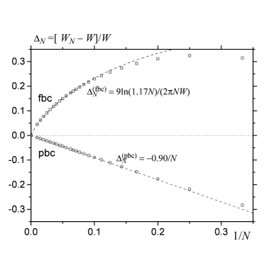
Fig. 1: Lattice sums $W_{N}$ for the systems of the cubic form with free and periodic boundary conditions. $W=1.51639$ is the bulk value for the sc lattice.

5 Numerical results

Here we present our numerical results for the temperature and field dependence of the intrinsic magnetisation $M$ and induced magnetisation $m$ for small magnetic systems with simple cubic lattice and cubic shape, subject to free and periodic boundary conditions (fbc and pbc). As was mentioned in Sec. 2, the numerical method for solving the $D\to\infty$ model consists in obtaining the correlation function $s_{ij}$ and magnetisation $m_{i}$ from the linear equations (2.7), substituting them into the constraint equation (2.6), and solving the resulting nonlinear equation for the gap parameter $G_{i}$. On the first step we use a linear-equation solver based on the sparce-matrix storage appropriate for the Dyson matrix ${\cal D}$, which is defined by Eq. (2.7), in our case of nearest-neighbour interactions. The nonlinear problem is tackled using a nonlinear-equation solver of the Newton-Raphson kind. For the present geometry, symmetry arguments have been used to reduce the number of unknowns and thereby to increase the computing performance. The relevant subset of sites corresponding to different values of $G_{i}$ is obtained by taking 1/8 of the cube with a subsequent reduction by a factor of about 3! using permutations of the coordinates $x$, $y$, and $z$. This allows us to reduce the number of unknowns by a factor of about $8\times 3!=48$, this estimation becomes asymptotically exact for ${\cal N}\gg 1$. For the square lattice the reduction factor is about $4\times 2!=8$. All computations have been performed on a Pentium III/450 MHz of 128 MB RAM.

\begin{picture}(15.0,7.5)\centerline{\hbox{\psfig{angle=-90,width=284.52756pt}}} \end{picture}

Fig. 2: Temperature dependence of the intrinsic magnetization $M$, Eq. (2.11), and local magnetizations $M_{i}$, Eq. (2.15), of the $14^{3}$ cubic system with free and periodic boundary conditions in zero field.

\begin{picture}(15.0,6.5)\centerline{\hbox{\psfig{angle=-90,width=284.52756pt}}} \end{picture}

\begin{picture}(15.0,7.0)\centerline{\hbox{\psfig{angle=-90,width=284.52756pt}}} \end{picture}

Fig. 3: Magnetization profiles in the direction from the center of the cube to the center of a face at different temperatures $\theta\equiv T/T_{c}^{{\rm MFA}}$. The magnified lower plot shows the long-range character of the profile at low temperatures.

\begin{picture}(15.0,7.5)\centerline{\hbox{\psfig{angle=-90,width=284.52756pt}}} \end{picture}

Fig. 4: Finite-size-scaling plot for the magnetization of cubic systems with linear size $N=10$ and 14.

\begin{picture}(15.0,7.5)\centerline{\hbox{\psfig{angle=-90,width=284.52756pt}}} \end{picture}

Fig. 5: Field dependence of the intrinsic magnetization $M$ and intrinsic magnetization $m$ for hypercubic lattices with fbc in three and two dimensions. Dashed line is a plot of Eq. (2.13) in which $M(H,T)$ is replaced by its zero-field value. Bulk magnetization $m_{{\rm b}}$ in two and three dimensions is shown by solid lines.

Fig. 2 shows the temperature dependence of the intrinsic magnetisation $M$, Eq. (2.11), and local magnetisations $M_{i}$, Eq. (2.15), of the $14^{3}$ cubic system with free and periodic boundary conditions in zero field. For periodic boundary conditions, $M$ exceeds the bulk magnetisation at all temperatures. In particular, at low temperatures this is in accord with the positive sign of the finite-size correction to the magnetisation, Eqs. (3.31) and (3.22). The magnetisation at the center of the cube with free boundary conditions is rather close to that for the model with pbc in the whole temperature range and converges with the latter at low temperatures. Local magnetisations at the center of the faces and edges and those at the corners decrease with temperature much faster than the magnetisation at the center. This is also true for the intrinsic magnetisation $M$ which is the average of the local magnetisation $M_{i}$ over the volume of the system: For the relatively small size $14^{3}$ the contribution from the boundaries to the average properties are still substantial. One can see that, in the temperature range below the bulk critical temperature, $M$ is smaller than the bulk magnetisation. This means that the boundary effects suppressing $M$ are stronger than the finite-size effects which lead to the increase of the latter. This is also seen from the low-temperature expresion for $M$ given in Eq. (4.47).

Magnetization profiles in the direction from the center of the cube to the center of a face are shown in Fig. 3 at different temperatures. One can see that perturbations due to the free boundaries extend deep into the system. This is a consequence of the Goldstone mode which renders the correlation length of an isotropic bulk magnet infinite below $T_{c}$. The latter effect is better seen from the magnified data at the low temperature (see the lower plot), where the MFA predicts, on the contrary, a fast approach to a constant magnetisation when moving away from the surfaces [3]. MC simulations of the classical Heisenberg model [3, 4] also show long-range magnetisation profiles. The difference of the local magnetisations in the center and at a surface point reaches a maximun in the vicinity of the bulk $T_{c}$ and goes to zero at low and high temperatures.

Fig. 4 indicates that the critical indices for the magnetisation at the faces, edges, and corners are higher than the bulk critical index $\beta=1/2$ for the present $D=\infty$ model. The critical index at the face $\beta_{1}$ is the mostly studied surface critical index (see, for a review, Refs. [22, 23]). The exact solution of Bray and Moore [24] for the correlation functions at criticality in the $D=\infty$ model and application of the scaling arguments yield the value $\beta_{1}=1$ (see Table II in Ref. [22]). Exact values of the edge and corner magnetisation indices, $\beta_{2}$ and $\beta_{3}$, seem to be unknown for $D=\infty$. Cardy [25] used the first-order $\varepsilon$-expansion to obtain $\beta_{2}(\alpha)$ for the edge with an arbitrary angle $\alpha$. For $\alpha=\pi/2$ and $D=\infty$ in three dimensions the result for the edge critical exponent reads $\beta_{2}=13/8+O(\varepsilon^{2})=1.625+O(\varepsilon^{2})$.

To estimate the magnetisation critical indices in our model we have performed a finite-size-scaling analysis (see, for a review, Ref. [26]) assuming the scaling form $M=N^{-\beta/\nu}F_{M}(\tau N^{1/\nu})$ and plotting in Fig. 4 the magnetisation times $N^{\beta/\nu}$ vs $\tau N^{1/\nu}$. Here $\nu=1$ is the critical index for the correlation length in the bulk and $\tau\equiv T/T_{c}-1$, where $T_{c}=T_{c}^{{\rm MFA}}/W$ is the bulk Curie temperature. Our results for the systems with $N=10$ and $N=14$ merge into single “master curves” for $\beta_{1}=0.86$, $\beta_{2}=1.33$, and $\beta_{3}=1.79$, which have been obtained by fitting $M\propto N^{-\beta/\nu}$ at $T=T_{c}$, i.e., $\theta=\theta_{c}=1/W$. Note that our value 0.86 for the surface magnetisation critical index $\beta_{1}$ is substantially lower than the value $\beta_{1}=1$ following from scaling arguments. This disagreement is probably due to corrections to scaling which could be pronounced for our insufficiently large linear sizes $N=10$ and 14. A more efficient way for obtaining an accurate value of $\beta_{1}$ is to perform a similar analysis for the semi-infinite model. The latter was considered analytically and numerically for $T\geq T_{c}$ and $H=0$ in Ref. [14]. We also mention the Monte Carlo simulations of the Ising model [27] which yield $\beta_{1}=0.80$, $\beta_{2}=1.28$, and $\beta_{3}=1.77$.

The field dependence of $M$ and $m$ at fixed temperature, as obtained from the numerical solution of Eqs. (2.4) – (2.6), for cubic and square systems is shown in Fig. 5. Naturally the numerical results for $m$ confirm Eq. (2.13) which describes both the effect of orientation of the system’s magnetisation by the field and the increase of $M$ in field. On the contrary, using the zero-field value of $M$ in Eq. (2.13) leads to a poor result for $m$ shown by the dashed curve for the 10³ system in Fig. 5. Here we do see that there are two distinct field ranges separated by the characteristic field $h^{*}$, which were discussed at the end of Sec. 2. The results of Fig. 5 are in qualitative agreement with those of Fig. 1 in Ref. [18] showing the field dependence of $\chi=\partial m/\partial h$ obtained from phenomenological arguments. We would like to stress, however, that Eq. (2.13) which is exact in the $D=\infty$ model, has not yet been checked for systems with a finite number of spin components $D$ and arbitrary size ${\cal N}$. The field dependence of the particle’s magnetisation similar to that shown in Fig. 5 for the cubic system was experimentally obtained for ultrafine cobalt particles in recent Ref. [28], as well as in a number of previous experiments.

The curves for the square system in Fig. 5 illustrate the fact that in two dimensions thermal fluctuations are much stronger than in 3$d$, which leads to lower values of both $M$ and $m$ at the same temperature. The bulk magnetisation $m_{{\rm b}}$ in two dimensions vanishes at zero field and it thus goes below the intrinsic magnetisation $M$ in the low-field region.

6 Conclusion

In this paper, we have studied finite-size and boundary effects in small ferromagnetic systems with free boundaries within the $D=\infty$ classical vector model. This model, while sacrificing about 5% in the overall accuracy when used as a substitute for the Heisenberg model in three dimensions, is exactly solvable and describes relevant physical features related to the Goldstone modes, such as the absence of ordering in two dimensions for isotropic models, long-range magnetisation profiles, etc. The $D=\infty$ model is clearly superior to the mean field approximation which ignores these important effects.

An important result of our work is the exact relation in Eq. (2.13) beetween the intrinsic magnetisation $M(H,T)$ and induced magnetisation $m(H,T)$. It would be interesting to check whether this plausible relation holds for a more realistic Heisenberg model. In the latter case, it should be at least a good approximation.

Whereas the finite-size effects, which occur in a pure form in systems with periodic boundary conditions, lead to the insrease of the magnetisation with respect to the bulk value, boundary effects in systems with free boundaries work in the opposite direction. Since the magnetisation reduction caused by the boundaries extends over the whole system (i.e., the magnetisation profiles are long ranged), the boundary effect overweighs the finite-size effect by a large logarithmic contribution (see Fig. 1), and the resulting intrinsic magnetisation $M$ is lower than the bulk magnetisation below the bulk critical temperature. The latter effect and the long-range magnetisation profiles are illustrated in Figs. 2 and 3.

We have also attempted to estimate the surface magnetisation critical indices for the faces, edges, and corners of the cube from the scaling analysis of the data for cubic systems with linear sizes $N=10$ and $N=14$. It seems that our values for all these indices are too low and the data for larger sizes are needed. The required computer resources, however, rapidly increase with the system’s linear size $N$, since the theory operates with the correlation matrices of the size $N^{3}\times N^{3}$.

Field dependences of the particle’s induced magnetisation $m$ in Fig. 5 reflect both the alignment of the intrinsic magnetic moment $M$ by the field and the increase of $M$ in field. A combination of these two effects was observed in many experiments including the recent publication [28].

The present approach can be extended to magnetic systems of other shapes (spherical, cylindrical, etc.), more complicated lattice structures, and systems with a bulk and surface anisotropy. This will also allow us to compare with the results of the Monte Carlo simulations of a nanoparticle (of the maghemite type) studied in [4]. We are planning to study these issues in our future work.

References

- [1] J.-L. Dormann, D. Fiorani, and E. Tronc, Adv. Chem. Phys. 98, 283 (1997).
- [2] O. Eriksson, A. M. Boring, R. C. Albers, G. W. Fernando, and B. R. Cooper, Phys. Rev. B 45, 2868 (1992).
- [3] V. Wildpaner, Z. Phys. B 270, 215 (1974).
- [4] H. Kachkachi, A. Ezzir, M. Noguès, and E. Tronc, Eur. Phys. J. B14 (2000) 681.
- [5] H. E. Stanley, Phys. Rev. Lett. 20, 589 (1968).
- [6] H. E. Stanley, Physics Reports 176, 718 (1968).
- [7] T. N. Berlin and M. Kac, Physics Reports 86, 821 (1952).
- [8] M. N. Barber and M. E. Fisher, Ann. Phys. (N.Y.) 77, 1 (1973).
- [9] H. J. F. Knops, J. Math. Phys. 14, 1918 (1973).
- [10] G. Costache, D. Mazilu, and D. Mihalache, J. Phys. C 9, L501 (1976).
- [11] D. A. Garanin, Z. Phys. B 102, 283 (1997).
- [12] D. A. Garanin, J. Phys. A 29, 2349 (1996).
- [13] D. A. Garanin, J. Phys. A 29, L257 (1996); 32, 4323 (1999).
- [14] D. A. Garanin, Phys. Rev. E 58, 254 (1998).
- [15] D. A. Garanin and V. S. Lutovinov, Solid State Commun. 50, 219 (1984).
- [16] D. A. Garanin, J. Stat. Phys. 74, 275 (1994).
- [17] D. A. Garanin, Phys. Rev. B 53, 11593 (1996).
- [18] M. E. Fisher and V. Privman, Phys. Rev. B 32, 447 (1985).
- [19] M. E. Fisher and V. Privman, Commun. Math. Phys. 103, 527 (1986).
- [20] W. Döring, Z. Naturforsch. 16a, 1008 (1961).
- [21] P. V. Hendriksen, S. Linderoth, and P.-A. Lindgard, Phys. Rev. B 48, 7259 (1993).
- [22] K. Binder, in Phase Transitions and Critical Phenomena, edited by C. Domb and J. L. Lebowitz (Academic Press, New York, 1983), Vol. 8.
- [23] H. W. Diehl, in Phase Transitions and Critical Phenomena, edited by C. Domb and J. L. Lebowitz (Academic Press, London, 1986), Vol. 10, pp. 75–267.
- [24] A. J. Bray and M. A. Moore, Phys. Rev. Lett. 38, 735 (1977); J. Phys. A 10, 1927 (1977).
- [25] J. L. Cardy, J. Phys. A 16, 3617 (1983).
- [26] K. Binder, in Computational Methods in Field Theory, edited by H. Gausterer and C. B. Lang (Springer, Berlin, 1992).
- [27] M. Pleimling and W. Selke, Eur. Phys. J. B. 5, 805 (1998); Phys. Rev. E 61, 933 (2000).
- [28] M. Respaud, J. M. Broto, H. Rakoto, A. R. Fert, L. Thomas, B. Barbara, M. Verelst, E. Snoeck. P. Lecante, A. Mosset, J. Osuna, T. Ould Ely, C. Amiens, and B. Chaudret, Phys. Rev. B 57, 2925 (1998).