Eur. Phys. J. B 22, 291–300 (2001)





Spin-wave theory for finite classical magnets
and superparamagnetic relation

Abstract

Analytical calculations based on finite-size spin-wave theory and Monte Carlo (MC) simulations are performed to investigate the validity of the well-known relation $m(H,T)=M(H,T)B_{D}[M(H,T){\cal N}H/T]$ between the induced magnetization $m$ of the magnetic particle and its intrinsic magnetization $M$ for the Ising and isotropic classical models [$B_{D}(x)$ is the Langevin function, $D$ is the number of spin components, ${\cal N}$ is the number of atoms in the particle]. It follows from general arguments and from our analytical results for the Heisenberg model at $T\ll T_{c}$ that this relation is not exact for any finite $D$ and nonzero temperature. Nevertheless, corrections to this formula remain very small practically in the whole range $T<T_{c}$ if ${\cal N}\gg 1$, as confirmed by our Monte Carlo calculations. At $T\lesssim T_{c}/4$ there is a good agreement between the MC and finite-size spin-wave calculations for the field dependence of $m$ and $M$ for the Heisenberg model with free boundary conditions.

1 Introduction

For magnetic particles of a finite size one can generally define two magnetizations, $m$ and $M,$ the relation between which is frequently written in the form

$$m=MB_{D}(Mx),\qquad x\equiv{\cal N}H/T,$$ (1)

where $B_{D}(x)$ is the Langevin function [$B_{D}(x)=B_{3}(x)=\coth x-1/x$ for the isotropic Heisenberg model and $B_{D}(x)=B_{1}(x)=\tanh x$ for the Ising model] and ${\cal N}$ is the number of magnetic atoms in the system. Here $m$ is the magnetization induced by the magnetic field and microscopically defined as the thermodynamic average of the vector

$${\bf M}=\frac{1}{{\cal N}}\sum_{i}{\bf s}_{i},$$ (2)

i.e.,

$${\bf m}=\langle{\bf M}\rangle.$$ (3)

For classical systems discussed throughout this paper, ${\bf s}_{i}$ can be considered, up to a factor, as spin vectors of unit length, $|{\bf s}_{i}|=1.$ The magnetization $M$ in Eq. (1) can be interpreted as the intrinsic magnetization of the particle which is defined through the correlation function of the magnetic moments,

$$M=\sqrt{\left\langle{\bf M}^{2}\right\rangle}$$ (4)

If the temperature is low, all spins in the particle are bound together by the exchange interaction and ${\bf M}$ behaves as a rigid “giant spin”, $|$${\bf M|\cong}M{\bf\cong}1,$which shows a superparamagnetic behavior. If a magnetic field ${\bf H}$ is applied, ${\bf M}$ exibits an average in the direction of ${\bf H,}$ which leads to a nonzero value of the induced magnetization ${\bf m}$ given, obviously, by Eq. (1). The question of principal interest is, however, the field dependence of $M$ at nonzero temperatures, which can be responsible for deviations from the simple superparamagnetic behaviour of Eq. (1).

Early Monte Carlo (MC) simulations by Wildpaner wil74 for the classical Heisenberg model, where both magnetizations were determined independently as functions of field at different temperatures, confirmed Eq. (1) within numerical errors. However, from the theoretical point of view this relation with $M=M(H,T)$ is unexpected.

On the theoretical side, Eq. (1) was obtained in Ref. hasleu90 for a classical model and in Ref. hasnie93 for a quantum model but without the field dependence of $M$. Earlier, Fisher and Privman fispri85 considered the spin-wave contribution to Eq. (1) but, again, the field dependence of $M$ was not studied explicitly.

Experimentally, the field dependence of $M$ and, in particular, the nonsaturation of the magnetization in the region $x\gtrsim 1$ have been observed in nanoparticles by different groups dorfiotro97 ; chesorklahad95 ; resetal98 . Usually this dependence is close to linear and is used to extract the value of $M$ at zero field by extrapolation to $H=0$. For the isotropic Heisenberg model, the field dependence of $M$ in the range $x\gtrsim 1$ is due to suppression of the fluctuations of individual spins, i.e., of spin waves, and this dependence disappears for $T\rightarrow 0$. The dependence $M(H)$ is much stronger and persists at zero temperatures if the spins in the particle are not perfectly collinear due to surface effectsresetal98 .

In our recent paper kacgar01 (see also Ref. kacnogtrogar00 ) we have shown that this relation becomes exact for the exactly solvable model of the $D$-component classical vector “spins” in the limit $D\rightarrow\infty$. Nevertheless, for more realistic models such as the classical Heisenberg model ($D=3$) and the Ising model ($D=1$), it is very difficult to believe that the superparamagnetic relation holds for all temperatures. Clearly, if the number ${\cal N}$ of atoms in the particle is large and the temperature is below $T_{c}$, then the argument of the Langevin function in Eq. (1) becomes large already for so small fields that $M$ does not essentially deviate from its zero-field value. Under these conditions Eq. (1) should be a good approximation. On the other hand, for smaller particles and near or above $T_{c},$ there should be deviations from the simple behavior, the study of which is the purpose of this work.

The structure of the rest of this article is as follows. In Sec. 2 using the low-field expansion of $m$ and general arguments we show that Eq. (1) is not exact for any finite value of $D$ and nonzero temperatures. In particular, in the high-temperature limit there is another analytic form of Eq. (1) with $B_{D}$ substituted by $B_{\infty}$. In Sec. 3 we present an explicit calculation of both $m(H,T)$ and $M(H,T)$ at low temperatures with the help of a spin-wave theory which separates the global-rotation mode and the ${\bf k}\neq{\bf 0}$ spin-wave modes. In Sec. 4 we perform high-accuracy MC simulations for the Ising and classical Heisenberg models in the box geometry to illustrate the superparamagnetic behavior in a wide range of parameters.

2 Basic Relations

We use the classical spin-vector Hamiltonian

$${\cal H}=-{\bf H}\sum_{i}{\bf s}_{i}-\frac{1}{2}\sum_{ij}J_{ij}{\bf s}_{i}\cdot{\bf s}_{j},\qquad|{\bf s}_{i}|=1,$$ (5)

where ${\bf s}$ is a $D$-component vector ($D=1$ for the Ising model and $D=3$ for the Heisenberg model). For this Hamiltonian one can prove an identity relating correlations functions and susceptibilities

$$M^{2}=m^{2}+\frac{dm}{dx}+\frac{(D-1)m}{x},$$ (6)

where $x$ is given by Eq. (1). On the right-hand side of Eq. (6), the second and third terms are contributions from the longitudinal and $D-1$ transverse susceptibilities, respectively. This relation can be used to extract the value of $M(H,T)$ from measurements of the induced magnetization $m$ and susceptibilities. Let us demonstrate how it works at low fields, where the expansion of $m$ can be written as

$$m\cong\frac{a^{2}}{D}x-\frac{c^{4}}{D^{2}(D+2)}x^{3}.$$ (7)

Applying Eq. (6) one readily obtains

$$M\cong a+\frac{a^{4}-c^{4}}{2aD^{2}}x^{2}.$$ (8)

At zero temperature the magnetic moment of the particle can be considered as a rigid spin, thus in Eq. (7) $a=c=1$ which results in $M=1,$ independently of the field. At $T>0$ one has $a<1$ and $c<a,$ so that $M$ increases with the field. The coefficients $a$ and $c$ can be calculated analytically at low and high temperatures [see, e.g., Eq. (60)]. Let us check now what happens if we try to find $M$ from Eq. (1) under the same conditions. One can write

$$m\cong\frac{M^{2}}{D}x-\frac{M^{4}}{D^{2}(D+2)}x^{3},\qquad M\cong M_{0}+M_{2}x^{2},$$ (9)

and find the coefficients $M_{0}$ and $M_{2}$ from the condition that $m$ here coinsides with that of Eq. (7). The result is Eq. (8) with $D^{2}\rightarrow D(D+2).$ This is clearly a wrong result for any finite value of $D$ and nonzero temperature. Only in the limit $T\rightarrow 0$ the coefficient $M_{2}$ vanishes and both approaches yield the same trivial result. Therefore, one cannot use Eq. (1) to take into account the field variation of $M$ in the range where the argument of $B$ is of order one or less. This formula can only be correct in the case of large particles for which the change of $M$ in this field range is very small and $M$ actually changes for much larger fields where we already have $m\cong M.$

On the other hand, using these results one can find the correction to Eq. (1) at low fields. To this end, one can write

$$m=MB(Mx)+\delta,$$ (10)

expand it for $x\ll 1$ using Eq. (8) and equate the result to Eq. (7) to find $\delta$. The result is

$$\delta=-\frac{2(a^{4}-c^{4})}{D+2}\frac{x^{3}}{D^{3}}<0,$$ (11)

that is, the Langevin function $B_{D}$ in Eq. (1) should be replaced by some function $F$ which goes below $B_{D}$ at nonzero temperatures.

In the high-temperature limit one can find an explicit form of the superparamagnetic relation which also differs from Eq. (1). Indeed, at high temperatures the exchange interaction can be neglected and one has to solve a one-spin problem, which yields

$$m=B(\xi),\qquad M^{2}=m^{2}+\frac{1}{{\cal N}}\left(B^{\prime}(\xi)+(D-1)\frac{B(\xi)}{\xi}\right),$$ (12)

where $\xi\equiv H/T.$ Using this relation, one can plot $\ m/M$ vs $x_{M}\equiv Mx$ and thus obtain the scaling function $F(x)$ which replaces $B_{D}(x)$ in Eq. (1). For large particles, ${\cal N}\gg 1,$ in the relevant region $x_{M}\sim 1$ one has $\xi\ll 1$ and the second of Eqs. (12), with the use of $B^{\prime}(\xi)\cong B(\xi)/\xi\cong 1/D,$ simplifies to

$$M^{2}=m^{2}+Dm/x.$$ (13)

On the other hand, this relation holds in the large-$D$ limit for all temperatures, particle sizes, and types of boundary conditions, and it can be obtained from Eq. (6) by dropping the term $dm/dx$ and replacing $D-1\rightarrow D.$ Solving this equation for $m$ yields the scaling function of the spherical model

$$F(x)=B_{\infty}(x)=\frac{2x/D}{1+\sqrt{1+(2x/D)^{2}}},$$ (14)

in Eq. (1) which goes below $B_{D}(x)$ for any finite $D.$

3 Spin-wave theory for finite-size magnetic particles

3.1 General

At low temperatures all spins in the particle are strongly correlated and they form a “giant spin” ${\bf M}$ [see Eq. (2)] which behaves superparamagnetically. In addition, there are internal spin-wave excitations in the particle which are responsible at nonzero temperatures for the fact that $M<1$ and for the field dependence of $M$. In our case of three-dimensional particles, $d=3$, these excitations can be described perturbatively in small deviations of individual spins ${\bf s}_{i}$ from the direction of ${\bf M.}$ To this end, it is convenient to insert an additional integration over $d{\bf M}=M^{D-1}dMd{\bf n}$ in the partition function,

$${\cal Z}=\int M^{D-1}dMd{\bf n}\prod_{i}d{\bf s}_{i}\delta\left({\bf M-}\frac{1}{{\cal N}}\sum_{i}{\bf s}_{i}\right){\rm e}^{-{\cal H}/T},$$ (15)

and first integrate over the magnitude $M$ of the central spin [this variable appears locally and it should not be confused with the intrinsic magnetization $M$ defined by Eq. (4)]. To do this, one should reexpress the vector argument of the $\delta$-function in the coordinate system specified by the direction of the central spin ${\bf n}$, which yields

$$\delta\left({\bf M-}\frac{1}{{\cal N}}\sum_{i}{\bf s}_{i}\right) = \delta\left(M{\bf-}\frac{1}{{\cal N}}\sum_{i}({\bf n\cdot s}_{i})\right)$$ (16)

$$\times\delta\left(\frac{1}{{\cal N}}\sum_{i}\left[{\bf s}_{i}-{\bf n}({\bf n\cdot s}_{i})\right]\right).$$

Then after integration over $M$ one obtains

$${\cal Z}=\int d{\bf n}{\cal Z}_{{\bf n}},$$ (17)

where

$${\cal Z}_{{\bf n}}=\int\prod_{i}d{\bf s}_{i}\delta\left(\frac{1}{{\cal N}}\sum_{i}\left[{\bf s}_{i}-{\bf n}({\bf n\cdot s}_{i})\right]\right){\rm e}^{-{\cal H}_{{\rm eff}}/T}$$ (18)

and

$${\cal H}_{{\rm eff}} = -({\bf n\cdot H})\sum_{i}({\bf n\cdot s}_{i})-\frac{1}{2}\sum_{ij}J_{ij}{\bf s}_{i}\cdot{\bf s}_{j}$$ (19)

$$-(D-1)T\ln\left[\frac{1}{{\cal N}}\sum_{i}{\bf n\cdot s}_{i}\right].$$

In Eq. (18), the $\delta$-function expresses the obvious condition that the sum of all spins does not have a component perpendicular to the central spin ${\bf M}$. This will lead to the absence of the zero Fourier component of the transverse fluctuations of spins in the particle. The corresponding global-rotation Goldstone mode (which is troublesome in the standard spin-wave theory for finite systems) has been transformed into the integration over the global variable ${\bf n}$ in Eq. (17) in the present formalism. The condition mentioned above was also used to transform the Zeeman term in Eq. (19). This describes now the spins ${\bf s}_{i}$ in a field in the direction ${\bf n}$ and with the strength ${\bf n\cdot H}$. As we will see below, the last term in Eq. (19) is nonessential in the leading approximation at low temperatures.

To calculate ${\cal Z}_{{\bf n}}$ at low temperatures, one can expand ${\cal H}_{{\rm eff}}$ up to the bilinear terms in the transverse spin components

$${\bf\Pi}_{i}\equiv{\bf s}_{i}-{\bf n}({\bf n\cdot s}_{i})$$ (20)

using

$${\bf n\cdot s}_{i}=\sqrt{1-{\bf\Pi}_{i}^{2}}\cong 1-{\bf\Pi}_{i}^{2}/2.$$ (21)

This yields

$${\cal H}_{{\rm eff}} \cong E_{0}-{\cal N}{\bf n\cdot H}+\frac{1}{2}\sum_{ij}A_{ij}{\bf\Pi}_{i}\cdot{\bf\Pi}_{j},$$

$$A_{ij} \equiv \left[(D-1)T/{\cal N}+{\bf n\cdot H+}\sum_{l}J_{il}\right]\delta_{ij}-J_{ij},$$ (22)

where $E_{0}=-(1/2)\sum_{ij}J_{ij}$ is the zero-field ground-state energy. For the lattice sites inside the particle or for the model with periodic boundary conditions one has $z=2d,$ where $d$ is the spatial dimension; for the sites on the boundaries $z_{i}<2d.$ Now ${\cal Z}_{{\bf n}}$ in Eq. (18) takes on the form

$${\cal Z}_{{\bf n}} \cong {\rm\exp}\left(\frac{-E_{0}+{\cal N}{\bf n\cdot H}}{T}\right){\cal N}^{D-1}\int_{-\infty}^{\infty}\prod_{i}\prod_{\alpha=1}^{D-1}d\Pi_{i}^{\alpha}\,$$ (23)

$$\times\delta\left(\sum_{i}{\bf\Pi}_{i}\right)\exp\left(-\frac{1}{2T}\sum_{ij}A_{ij}{\bf\Pi}_{i}\cdot{\bf\Pi}_{j}\right),$$

which after working out the Gaussian integral over $\Pi_{i}^{\alpha}$ yields

$${\cal Z}_{{\bf n}}\cong{\rm\exp}\left(\frac{-E_{0}+{\cal N}{\bf n\cdot H}}{T}\right){\cal N}^{D-1}\left[\frac{(2\pi T)^{{\cal N}-1}}{\det A_{ij}^{\prime}}\right]^{(D-1)/2},$$ (24)

where the matrix $A_{ij}^{\prime}$ is obtained from $A_{ij}$ of Eq. (22) by elimination of ${\bf\Pi}_{i}$ on one of the ${\cal N}$ lattice sites using the condition $\sum_{i}{\bf\Pi}_{i}=0.$

Eq. (24) is a general result which is valid for a particle of arbitrary shape and for different types of exchange interaction $J_{ij}$ and boundary conditions. In the following subsection we will consider particles of cubic shape with the nearest-neighbour interactions and free and periodic boundary conditions (fbc and pbc).

3.2 Free and periodic boundary conditions

Let us express the matrix $A_{ij}$ through its eigenfunctions $f_{ki}$ as follows

$$A_{ij}=\sum_{k}f_{ki}^{*}A_{k}f_{kj},$$ (25)

where $f_{ki}$ satisfy

$$\sum_{i}f_{ki}A_{ij}=A_{k}f_{kj}$$ (26)

and form an orthonormal and complete basis

$$\sum_{i}f_{ki}^{*}f_{k^{\prime}i}=\delta_{kk^{\prime}},\qquad\sum_{k}f_{ki}^{*}f_{ki^{\prime}}=\delta_{ii^{\prime}}.$$ (27)

In this basis, the sum over $ij$ in Eq. (23) can be rewritten as

$$\sum_{ij}A_{ij}{\bf\Pi}_{i}\cdot{\bf\Pi}_{j}=\sum_{k}A_{k}{\bf\Pi}_{k}^{*}\cdot{\bf\Pi}_{k},$$ (28)

where

$${\bf\Pi}_{k}\equiv\sum_{i}f_{ki}{\bf\Pi}_{i}.$$ (29)

Now one can make the observation that in the set of eigenfunctions $f_{ki}$ there is one which is independent of $i$ and which can be conveniently ascribed to $k=0$, i.e., $f_{0}=1/{\cal N}$. This follows since

$$\sum_{i}A_{ij}=A_{0}=(D-1)T/{\cal N}+{\bf n\cdot H}$$ (30)

is independent of $j$, $A_{0}$ being the zero-$k$ eigenvalue. Now one can see that $\delta\left(\sum_{i}{\bf\Pi}_{i}\right)$ in Eq. (23) excludes integration over the zero mode ${\bf\Pi}_{0}$ in the new representation. Fluctuations of the components ${\bf\Pi}_{k}$ with $k\neq 0$ yield multiplicative contribitions to the partition function, so that one is left with the integrals over $\Pi_{k}^{\alpha}$. If the eigenfunctions $f_{ki}$ are real, one obtains

$$I_{k}^{\alpha}=\int_{-\infty}^{\infty}d\Pi_{k}^{\alpha}\exp\left[-\frac{A_{k}}{2T}(\Pi_{k}^{\alpha})^{2}\right]=\left(\frac{2\pi T}{A_{k}}\right)^{1/2}.$$ (31)

If $f_{ki}$ are complex, one has to integrate independently over the real and imaginary components $x_{k}^{\alpha}$ and $y_{k}^{\alpha}$ of $\Pi_{k}^{\alpha}=x_{k}^{\alpha}+iy_{k}^{\alpha}$ which gives $2\pi T/A_{k}$. Complex eigenfunctions arise, however, only in the case of periodic boundary conditions where, as we shall see, one has to take into account only a half of the $k$ modes, which effectively restores the result of Eq. (31). So let us consider for the moment only systems with real eigenfunctions. In this case, integrating over $({\cal N}-1)(D-1)$ modes (${\cal N}-1$ $k$-modes multiplied by $D-1$ transverse spin components) for ${\cal Z}_{{\bf n}}$ one obtains Eq. (24) with

$$\det A_{ij}^{\prime}=\prod_{k}{}^{{}^{\prime}}\frac{A_{k}}{\cal N},$$ (32)

where the prime on the product means that the mode with $k=0$ is omitted.

All the results above are still general. Now we will consider cubic-shaped particles with free and periodic boundary conditions. In the fbc case the matrix $A_{ij}$ has the form

$$A_{ij}=A_{0}\delta_{ij}+\Delta_{ij}^{(x)}+\Delta_{ij}^{(y)}+\Delta_{ij}^{(z)},$$ (33)

where $A_{0}$ is given by Eq. (30) and

$$\Delta_{ij}^{(x)}=-J[\delta_{i_{x},j_{x}-1}+\delta_{i_{x},j_{x}+1}-\delta_{i_{x},j_{x}}(2-\delta_{j_{x},1}-\delta_{j_{x},N})]$$

$$\qquad\qquad{}\times\delta_{i_{y},j_{y}}\delta_{i_{z},j_{z}},$$ (34)

etc., $\delta_{i_{x},j_{x}}$ are Kronecker symbols, and $i_{x},j_{x}=1,\ldots,N$. If $j_{x}-1$ or $j_{x}+1$ run out of the particle, the corresponding $\delta_{i_{x},j_{x}-1}$ or $\delta_{i_{x},j_{x}+1}$ should be omitted. One can see that $\Delta_{ij}^{(x)}$ is a discrete Laplace operator for the coordinate $x$, and the eigenvalue problem factorizes. The eigenfunctions are standing waves and they can be written in the form

$$f_{{\bf k}i}=f_{i_{x},k_{x}}\times f_{i_{y},k_{y}}\times f_{i_{z},k_{z}},$$ (35)

where for $\alpha=x,y,z$

$$f_{i_{\alpha},k_{\alpha}}=\sqrt{\frac{2}{(1+\delta_{k_{\alpha},0})N}}\cos[(i_{\alpha}-1/2)k_{\alpha}],$$ (36)

$$k_{\alpha}=\pi n_{\alpha}/N,\qquad n_{\alpha}=0,1,\ldots,N-1.$$

For the eigenvalue $A_{k}$ one obtains

$$A_{\bf k}=A_{0}+J_{\bf k}-J_{0}.$$ (37)

In the case of periodic boundary conditions, one should drop the terms $\delta_{j_{x},1}$ and $\delta_{j_{x},N}$ and identify $i_{x}=N+1$ with $i_{x}=1$ in Eq. (3.2). The eigenfunctions can be conveniently taken in the form of plane waves $e^{-i{\bf kr}_{i}}$ with the wave vectors quantized as $k_{\alpha}=2\pi n_{\alpha}/N$, the eigenvalue $A_{\bf k}$ having the same form as in the fbc case. That is, the pbc and fbc models differ only by the quantization of the wave vector

$$k_{\alpha}=\left\{\begin{array}[]{cc}2\pi n_{\alpha}/N,&{\rm pbc}\\ \pi n_{\alpha}/N,&{\rm fbc}\end{array}\right.,\qquad n_{\alpha}=0,1,...,N-1$$ (38)

where $\alpha=x,y,z.$ This subtle difference is responsible for much stronger thermal fluctuations in the fbc model due to surface effects, as we shall see below.

3.3 The partition function

Collecting the formulae obtained above, one can write down the expession for ${\cal Z}_{{\bf n}}$ in the form

$${\cal Z}_{{\bf n}}\cong\tilde{A}{\rm\exp}\left({\bf n\cdot x}+{\cal N}\frac{D-1}{2}f(G_{{\bf n}})\right),$$ (39)

where $\tilde{A}$ is given by the first line of Eq. (56) below,

$${\bf x}\equiv{\cal N}{\bf H/}T$$ (40)

is the reduced field, the function $f(G_{{\bf n}})$ is defined by

$$f(G_{{\bf n}})\equiv\frac{1}{{\cal N}}\sum_{{\bf k}}{}^{{}^{\prime}}\ln\frac{G_{{\bf n}}}{1-G_{{\bf n}}\lambda_{{\bf k}}},$$ (41)

with $\lambda_{{\bf k}}\equiv J_{{\bf k}}/J_{0}=(\cos k_{x}+\cos k_{y}+\cos k_{z})/d,$ and

$$G_{{\bf n}}\equiv\frac{1}{1+a_{{\bf n}}}\cong 1-a_{{\bf n}},\quad a_{{\bf n}}\equiv\frac{T}{{\cal N}J_{0}}({\bf n\cdot x+}D-1)\ll 1.$$ (42)

Note that the angular dependence of ${\cal Z}_{{\bf n}}$ is more complicated than that for rigid spins because of the internal spin-wave modes described by the last term in Eq. (39). These SW modes have a gap accounted for by the first two terms in the denominator of Eq. (32) or the dimensionless parameter $a_{{\bf n}}$ in Eq. (42). One contribition to the gap is due to the finite size of the particle and the other is due to the magnetic field. The latter depends on the orientation of the particle’s magnetic moment ${\bf n}$ with respect to the field.

The function $f(G_{{\bf n}})$ of Eq. (41) can be written as

$$f(G_{{\bf n}})=f(1)-\int_{G_{{\bf n}}}^{1}du\frac{\widetilde{P}_{N}(u)}{u},$$ (43)

where $f(1)$ is a constant and

$$\widetilde{P}_{N}(G)\equiv\frac{1}{{\cal N}}\sum_{{\bf k}}{}^{{}^{\prime}}\frac{1}{1-G\lambda_{{\bf k}}}$$ (44)

is the lattice Green function. Since at low temperatures the argument $G$ in the expressions above is close to 1, it is convenient to write

$$\widetilde{P}_{N}(G) = \widetilde{P}_{N}(1)-\frac{1}{{\cal N}}\sum_{{\bf k}}{}^{{}^{\prime}}\frac{(1-G)\lambda_{{\bf k}}}{(1-G\lambda_{{\bf k}})(1-\lambda_{{\bf k}})}$$

$$= W_{N}-N(1-G)f_{P}(1-G),$$ (45)

where $W_{N}\equiv\widetilde{P}_{N}(1).$ Here, if the linear size $N$ is not large, one can replace $G\rightarrow 1$ in the argument of the function $f_{P}.$ For $N\gg 1$ the situation becomes more complicated since the wave vectors ${\bf k}$ come closer to the origin and a singularity is formed. For the system with free boundary conditions, the sum is dominated by $k\ll 1,$ so that $\lambda_{{\bf k}}\cong 1-k^{2}/(2d)$ and $f_{P}(y)$ has the form

$$f_{P}(y)\cong\frac{(2d)^{2}}{\pi^{4}}\sum_{n_{x},n_{y},n_{z}=0}^{\infty}{}^{{}^{\prime}}\frac{1}{(y+n^{2})n^{2}}$$ (46)

with $n^{2}=n_{x}^{2}+n_{y}^{2}+n_{z}^{2}$ and

$$y\equiv 2d(1-G)(N/\pi)^{2}.$$ (47)

For $y\ll 1$ one can set $y=0$ which yields $f_{P}(y)\cong f_{P}(0)=c_{{\rm fbc}}\simeq 1.90,$ whereas for $y\gg 1$ one can replace summation by integration and calculate the integral analytically. For the model with periodic boundary conditions, there are different contributions from different corners of the Brillouin zone in Eq. (45), and one obtains a more cumbersome analogue of Eq. (46). In practice, it is easier to compute $f_{P}$ from its definition in Eq. (45). For three-dimensional cubic particles the limiting cases are ($1-G\ll 1)$

$$\widetilde{P}_{N}(G)\cong W_{N}-\left\{\begin{array}[]{ll}c_{N}N(1-G),&y\ll 1\\ c_{0}\sqrt{1-G},&y\gg 1,\end{array}\right.$$ (48)

where for l$\arg$e $N$ the value of $W_{N}$ approaches the Watson integral $W=1.51639$ according to kacgar01

$$\Delta_{N}\equiv\frac{W_{N}-W}{W}\cong\left\{\begin{array}[]{ll}\displaystyle-\frac{0.90}{N},&{\rm pbc}\\ \displaystyle\frac{9\ln(1.17N)}{2\pi WN},&{\rm fbc}\end{array}\right.$$ (49)

(notice the positive sign for the fbc model). For the simple cubic lattice $c_{0}=(2/\pi)(3/2)^{3/2}$. The numerically obtained results for $c_{N}$ can, for $N\gg 1,$ be fitted as

$$c_{N}\cong\left\{\begin{array}[]{ll}0.384-1.05/N,&{\rm pbc}\\ 1.90-1.17/N,&{\rm fbc}\end{array}\right.$$ (50)

(see Fig. 1). The square-root term in Eq. (48) describes the spin-wave singularity in the infinite system. From Eqs. (47) and (42) it follows that the crossover to the bulk spin-wave behavior occurs for the values of the reduced field $x\gtrsim x_{S}\sim NJ_{0}/T$ which is much larger than the value $x\sim x_{V}=1$ corresponding to the suppression of the global rotation of the particle’s magnetic moment. The actual crossover fields, in notations of Ref. fispri85 , are given by

$$H_{V}=\frac{T}{{\cal N}}\ll H_{S}=\frac{\pi^{2}}{2d}\frac{J_{0}}{{\cal N}^{2/3}},$$ (51)

that is, they are widely separated from each other in our case $T/(NJ_{0})\ll 1.$ Thus the result for the function $f(G_{{\bf n}})$ of Eq. (43), which with the help of Eq. (45) can be written as

$$f(G_{{\bf n}})\cong f(1)-a_{{\bf n}}W_{N}+N\int_{0}^{a_{{\bf n}}}da\,af_{P}(y_{a})$$ (52)

with $y_{a}\cong 2da(N/\pi)^{2},$ can be simplified in different field ranges.

\begin{picture}(11.0,5.7)\centerline{\hbox{\psfig{angle=-90,width=256.0748pt}}} \end{picture}

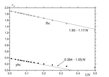
Figure 1: Finite-size effect on $c_{N}\equiv f_{P}(0)$ [see Eq. (45)] for cubic systems with free and periodic boundary conditions.

For $H\ll H_{S}$ one can replace $f_{P}(y_{a})$ by $c_{N}$ to obtain, in Eq. (39),

$${\cal N}\frac{D-1}{2}f(G_{{\bf n}}) \cong {\cal N}\frac{D-1}{2}f(1)-t({\bf n\cdot x}+D-1{\bf)}$$ (53)

$$\qquad{\bf+\alpha}({\bf n\cdot x}+D-1{\bf)}^{2},$$

where

$$t\equiv\frac{D-1}{2}\frac{W_{N}T}{J_{0}},\qquad\alpha\equiv\frac{(D-1)c_{N}}{4N^{2}}\left(\frac{T}{J_{0}}\right)^{2}$$ (54)

are small parameters, $\alpha\ll t\ll 1.$ Since $\alpha x^{2}\sim(H/H_{S})^{2}\ll 1,$ one can expand the partition function ${\cal Z}$ of Eqs. (17) and (39) with respect to the last term of Eq. (53), which yields

$${\cal Z} \cong \tilde{A}^{\prime}\int_{-1}^{1}du(1-u^{2})^{(D-3)/2}$$ (55)

$$\times\exp\left\{\left[1-t+2\alpha(D-1)\right]ux\right\}\left[1+\alpha(ux)^{2}\right]$$

where

$$\tilde{A}^{\prime} = {\cal N}^{D-1}\left(2\pi{\cal N}T/J_{0}\right)^{(D-1)({\cal N}-1)/2}e^{-E_{0}/T}$$ (56)

$$\times e^{(D-1)[{\cal N}f(1)/2-t]}S_{D-1}$$

and $S_{D}=2\pi^{D/2}/\Gamma(D/2)$ is the surface of the $D$-dimensional unit sphere. In fact, we have left the term proportional to $\alpha ux$ in Eq. (55) not expanded for the sake of convenience. Integration in Eq. (55) results in

$${\cal Z}\cong{\cal Z}_{0}\{[1-t+2\alpha(D-1)]x\}+\alpha x^{2}\frac{d^{2}{\cal Z}_{0}}{dx^{2}},$$ (57)

where ${\cal Z}_{0}\{[1-t+2\alpha(D-1)]x\}$ is the partition function of the rigid magnetic moment with the magnitude reduced by the factor $1-t+2\alpha(D-1)$.

3.4 The superparamagnetic relation

Using

$$\frac{1}{{\cal Z}_{0}}\frac{d^{2}{\cal Z}_{0}}{dx^{2}}=B^{2}+B^{\prime}=1-\frac{(D-1)B}{x},$$ (58)

where $B=B(x)$ is the Langevin function, for the induced magnetization $m$ one obtains

$$m = \frac{d\ln{\cal Z}}{dx}\cong[1-t+2\alpha(D-1)]$$

$$\qquad\times B\{[1-t+2\alpha(D-1)]x\}$$

$$\qquad+\alpha[2x-(D-1)(B+xB^{\prime})]$$

$$\cong [1-t+\alpha(D-1)]$$ (59)

$$\times B\{[1-t+\alpha(D-1)]x\}+2\alpha x.$$

Expanding the expression for $m$ for $x\ll 1$ leads to Eq. (7) with the explicit values of the parameters

$$a^{2} = [1-t+\alpha(D-1)]^{2}+2\alpha D,\qquad$$

$$c^{4} = [1-t+\alpha(D-1)]^{4}.$$ (60)

Note that in the region $x\gg 1,$ where a rigid magnetic moment would saturate, $m$ continues to increase linearly as $m\cong 1-t+\alpha(D-1)+2\alpha x.$ This is due to the field dependence of the intrinsic magnetization $M$. The latter can be calculated from Eq. (6) which leads to

$$M\cong 1-t+\alpha(2D-1)+2\alpha xB(x).$$ (61)

This formula decribes a crossover from the quadratic field dependence of $M$ at low field, $x\ll 1,$ to the linear dependence at $x\gg 1.$

Now we are in a position to calculate the correction to Eq. (1) at low temperatures and $x\sim 1.$ To this end, one can write $m$ in the form of Eq. (10), expand it with respect to $\alpha\ll 1$ and equate to the expanded form of Eq. (1). This gives

$$\delta=\alpha\left[2x-(D+2xB)(B+xB^{\prime})\right],$$ (62)

which has a negative value. In particular, for $x\ll 1$ one has $\delta\cong-8\alpha x^{3}/[D^{2}(D+2)]$ [cf. Eq. (11)]. It can be shown that $\delta\rightarrow 0$ in the large-$D$ limit. Since $\alpha$ defined by Eq. (54) contains $N^{2}$ in the denominator, $\delta$ remains small even if $T\sim J_{0}.$ This is an indication that Eq. (1) is a very good approximation for not extremely small systems in the whole range below $T_{c}$. It can be shown that for $N\gg 1$ crossover to the high-temperature form of Eq. (1) specified by the function $B_{\infty}(x)$ of Eq. (14) occurs in a close vicinity of $T_{c}$.

At higher fields $H\sim H_{S}$ there is another crossover to the standard spin-wave-theory result for $M.$ Here one has $x\gg 1,$ thus the integral in Eq. (17) is dominated by ${\bf n\cdot x}\cong x.$ Replacing ${\bf n\cdot x}\rightarrow x$ in the last term of Eq. (52) one obtains

$${\cal Z} \cong {\cal Z}_{0}[(1-t)x]\exp\left[\frac{D-1}{2}{\cal N}^{4/3}\int_{0}^{a_{x}}da\,af_{P}(y_{a})\right]\qquad$$

$$a_{x} \cong xT/({\cal N}J_{0})=H/J_{0},$$ (63)

which yields

$$m\cong M\cong 1-\frac{D-1}{2}\frac{T}{J_{0}}\left[W_{N}-\frac{H}{J_{0}}Nf_{P}\left(\frac{H}{H_{S}}\right)\right],$$ (64)

where the function $f_{P}(y)$ is defined by Eq. (45) and $H_{S}$ is defined by Eq. (51).

Let us now write down the explicit forms of the field dependence of the intrinsic magnetization $M$ in the three different field regions

$$M\cong 1-t+\left\{\begin{array}[]{ll}\displaystyle\frac{D-1}{2D}c_{N}\left(\frac{HN^{2}}{J_{0}}\right)^{2},&H\ll H_{V}\\ \displaystyle\frac{D-1}{2}c_{N}\frac{NHT}{J_{0}^{2}},&H_{V}\ll H\ll H_{S}\\ \displaystyle\frac{D-1}{2}c_{0}\frac{T}{J_{0}}\left(\frac{H}{J_{0}}\right)^{1/2},&H_{S}\ll H\ll J_{0}.\end{array}\right.$$ (65)

Here $t\ll 1$ is defined by Eq. (54). In the second and third field ranges, the particle’s magnetic moment is fully oriented by the field, thus $m\cong M,$ the spin-wave gap in Eq. (32) has the value $H$, as in the bulk, and the field dependence of both magnetizations follows that of the function $\widetilde{P}_{N}(G)$ of Eqs. (45) or (48) with $1-G\cong H/J_{0}$ [see Eq. (42)]. The region $H\ll H_{V}$ in Eq. (65) is less trivial. Here the gap in Eq. (32) is ${\bf n\cdot H}$ and depends on the orientation of the particle’s magnetic moment which is not yet completely aligned by the field. Effectively one has in this region ${\bf n\cdot H\sim}H^{2},$ which leads to a quadratic field dependence of $M$. In fact, such a dependence at smallest fields already follows from general principles, see Sec. 2, and is pertinent to the Ising model as well.

To conclude this subsection, we introduce the orientation-dependent “macroscopic” particle’s magnetization ${\bf M}_{{\bf n}}$ according to

$${\bf M}_{{\bf n}}\equiv\frac{\partial\ln{\cal Z}_{{\bf n}}}{\partial{\bf x}},$$ (66)

where ${\cal Z}_{{\bf n}}$ and ${\bf x}$ are defined by Eqs. (18) and (40), respectively. Using this definition, for the induced magnetization ${\bf m\equiv\partial}{\ln{\cal Z}}/\partial{\bf x}$ one can write

$${\bf m}=\frac{\int d{\bf n\,M}_{{\bf n}}{\cal Z}_{{\bf n}}}{\int d{\bf n}{\cal Z}_{{\bf n}}}.$$ (67)

${\bf M}_{{\bf n}}$ can be interpreted as ${\bf M}$ of Eq. (4) with the spin-wave modes integrated out. From Eq. (39) one obtains

$${\bf M}_{{\bf n}}=\left[1-\frac{D-1}{2}\frac{T}{J_{0}}\frac{\widetilde{P}_{N}(G_{{\bf n}})}{G_{{\bf n}}}\right]{\bf n,}$$ (68)

which for $H\ll H_{S}$ can be written as

$${\bf M}_{{\bf n}}\cong\left[1-t+2\alpha({\bf n\cdot x}+D-1)\right]{\bf n.}$$ (69)

The magnitude of the particle’s magnetization, $M_{{\bf n}}\equiv|{\bf M}_{{\bf n}}|,$ depends on its orientation due to spin-wave effects. It attains its maximal value $1-t+2\alpha(x+D-1)$ if the particle’s magnetization is directed along the field ${\bf H}$ and its minimal value $1-t+2\alpha(-x+D-1)$ in the thermodynamically unfavorable state with magnetization against the field. It should be stressed that in order to obtain the explicit result for the induced magnetization, Eq. (59), from Eq. (67), one should know ${\cal Z}_{{\bf n}},$ so its calculation in the main part of this section is unavoidable. On the other hand, for the intrinsic magnetization $M$ it is sufficient to replace ${\cal Z}_{{\bf n}}\Longrightarrow\exp({\bf n\cdot x)}$ and use

$$M\cong\frac{\int d{\bf n\,}M_{{\bf n}}\exp({\bf n\cdot x)}}{\int d{\bf n}\exp({\bf n\cdot x)}}$$ (70)

which readily yields Eq. (61) up to a field-independent term ($\alpha\ll t)$.

3.5 Local magnetization

The formalism developed above can be applied to study inhomogeneities in the particle’s magnetization arising as a consequence of free boundaries. Since in zero field the standardly defined local induced magnetization ${\bf m}_{i}\equiv\langle{\bf s}_{i}\rangle$ of a finite-size particle vanishes, one has to introduce local intrinsic magnetization

$$M_{i}=\frac{1}{M}\left\langle{\bf s}_{i}\cdot\frac{1}{\cal N}\sum_{j}{\bf s}_{j}\right\rangle.$$ (71)

One can check the identity $(1/{\cal N})\sum_{i}M_{i}=M$ showing the self-consistency of the definition given above. Adding the expression within the brackets to the integrand of Eq. (15) and repeating all operations, one arrives at the final low-temperature result

$$M_{i}\cong 1-\frac{D-1}{2}\frac{T}{\cal Z}\int d{\bf n}{\cal Z}_{{\bf n}}\sum_{k}{}^{{}^{\prime}}\frac{|f_{ki}|^{2}}{A_{k}},$$ (72)

where $A_{k}$ and $f_{ki}$ are eigenvalues and eigenfunctions of the linear problem, see Eq. (26). The latter contain the information about inhomogeneities in the system. For periodic boundary conditions, one has $f_{ki}=e^{-i{\bf kr}_{i}}/\sqrt{N}$, so that $|f_{ki}|=\sqrt{1/N}$ and there are no inhomogeneities. Since the parameter $t$ defined by Eq. (54) is small, one can expand Eq. (72) to obtain, to the lowest order at low temperatures,

$$M_{i}\cong 1-\frac{(D-1)T}{2}\sum_{k}{}^{{}^{\prime}}\frac{|f_{ki}|^{2}}{A_{k}}.$$ (73)

Here one can check again $(1/{\cal N})\sum_{i}M_{i}=M$, where $M\cong 1-t$, according to Eq. (61). For cubic particles with free boundary conditions, one has $f_{ki}\approx\sqrt{2/N}$ at the boundary according to Eq. (36), which is larger than the bulk-averaged value. The biggest effect of the surface is naturally attained at the corners of the cube where $M_{i}\approx 1-8t$.

4 MC simulations and results

The classical Monte Carlo (MC) method based on the Metropolis algorithm is now a standard technique (see, e.g., Ref. binhee92 for details). The general idea is to simulate the statististics of a magnetic system by generating a Markov chain of spin configurations and taking an average over the latter. Each step of this chain (a MC step) is a stochastic transition of the system from one state to another, subjected to the condition of the detailed balance. Usually a MC step consists in generating a new trial orientation of a spin vector on a lattice site $i$ and calculating the ensuing energy change of the system $\Delta E.$ The trial confuguration is accepted as a new configuration if

$$\exp(-\Delta E/T)\geq{\cal R}(0,1),$$ (74)

where ${\cal R}(0,1)$ is a random number in the interval $(0,1)$, otherwise the old configuration is kept. As follows from Eq. (74), for $\Delta E\leq 0$ the trial orientation is accepted with a probability 1. The trial orientation can be a completely random orientation, or a random orientation in the vicinity of the initial orientation of the spin ${\bf s}_{i},$ which is more appropriate at low temperatures. For the Ising model, the trial orientation is generated by a flip of $s_{i}$ with a probability 1/2. The MC steps are performed sequentially or randomly for all lattice sites. This conventional version of the MC method is not efficient for systems of finite size at low temperatures and small fields, if one is interested in the induced magnetization $m$. The Boltzmann distribution over the directions of the particle’s magnetic moment ${\bf M}$ of Eq. (2) is achieved by rotations of ${\bf M}$ itself rather than by rotations of individual spins ${\bf s}_{i}.$ Indeed, each spin ${\bf s}_{i}$ is acted upon by the strong exchange field ${\bf H}_{E,i}=\sum_{j}J_{ij}{\bf s}_{j}\sim J_{0},$ and in the typical case $H\ll J_{0}$ all trial configurations with the direction of ${\bf s}_{i}$ significantly differing from that of its neighbors are rejected with a probability close to 1. Thus in the standard MC procedure directions of individual spins can only change little by little, and the resulting change of ${\bf M}$ is extremely slow. For the Ising model the situation is even worse since the spin geometry is discrete and there are no small changes of spin directions, whereas a flip of a single spin against the exchange field has an exponentially small probability. Hence if one starts in zero field with the configuration of all spins up or all spins down, the magnetization $m$ will practically never relax to zero. This drawback can be remedied by augmenting the procedure by a global rotation (GL) of the particle’s spins to a new trial direction of ${\bf M}$ and calculating the energy change. That is, before turning single spins on all lattice sites, one computes ${\bf M,}$ generates its new orientation ${\bf M}^{\prime}$ and obtains the energy difference

$$\Delta E=-{\cal N}{\bf H\cdot(M}^{\prime}-{\bf M).}$$ (75)

If the new orientation is accepted according to Eq. (74), one turns all spins ${\bf s}_{i}$ by an appropriate angle and proceeds with the standard Metropolis method recapitulated above. In small fields ($x\equiv{\cal N}H/T\lesssim 1$) relaxation of the induced magnetization $m$ becomes much slower than that of the intrinsic magnetization $M,$ and one needs much more MC steps to find the former than the latter with the same precision. If in the procedure each global rotation is coupled with subsequent turning of single spins on all lattice sites $i$, making enough global rotations to achieve a required precision for $m$ costs much more computer time for larger particle sizes. Thus a natural idea is to make many global rotations and gather the data for $m$ after each GL before proceeding to the conventional (single-spin) part of the Metropolis algorithm. This improved method is especially fast for the isotropic Heisenberg or Ising models where the energy change is given by Eq. (75) since, after ${\bf M}$ has been initially computed, each of its subsequent rotations and calculations of $\Delta E$ requires $O(1)$ operations. In contrast, for systems with anisotropy one has to perform a sum over all lattice sites for each orientation of ${\bf M,}$ i.e., to make $O({\cal N})$ operations.

Finally, we mention that for the Heisenberg model $5^{3}$ the running time of our programme with global rotations on a Pentium III/933 MHz is 160mn, for a precision of $10^{-4}-10^{-5}$ on the magnetisation.

\begin{picture}(11.0,5.7)\centerline{\hbox{\psfig{angle=-90,width=256.0748pt}}} \end{picture}

Figure 2: Field dependence of the intrinsic magnetization $M$ and the induced magnetization $m$ of the Ising model on the sc lattice with fbc for different temperatures.

\begin{picture}(11.0,5.7)\centerline{\hbox{\psfig{angle=-90,width=256.0748pt}}} \end{picture}

Figure 3: Field dependence of the intrinsic magnetization $M$ and the induced magnetization $m$ of the Heisenberg model on the sc lattice with fbc for different temperatures.

Figs. 2 and 3 show the results of our MC simulations for the Ising and Heisenberg models on a cubic lattice with size ${\cal N}=5^{3}$ and free boundary conditions. The intrinsic magnetization $M$ and induced magnetization $m$ are plotted vs the scaled field $x\equiv{\cal N}H/T$ for different temperatures. We used the bulk Curie temperatures $T_{c}=\theta_{c}T_{c}^{{\rm MFA}},$ where $T_{c}^{{\rm MFA}}=J_{0}/D$ is the mean-field Curie temperature and $\theta_{c}$ is 0.751 for the Ising model and 0.722 for the Heisenberg model. One can see that the particle’s magnetic moment is aligned and thus $m\sim M$ for $x\gtrsim 1,$ if $T\ll T_{c}.$ At $T\gg T_{c}$ the field alignes individual spins and this requires $H\gtrsim T,$ i.e., $x\gtrsim{\cal N}.$ The quadratic dependence of $M(H)$ at small fields, which is phenomenologically described by Eq. (8), manifests itself strongly at elevated temperatures. At low temperatures this dependence is much more difficult to see on the graph because the field-dependent part of $M,$ which for the Heisenberg model is given by Eq. (61), is for $x\sim 1$ proportional to $\alpha$ of Eq. (54), which is very small. For the Ising model there is practically no field dependence of $M$ at low temperatures since $M$ is very close to 1. The weak linear field dependence of $M$ for the Heisenberg model which is visible on Fig. 2 at $T=T_{c}/4$ will be quantitatively explained below.

\begin{picture}(11.0,5.7)\centerline{\hbox{\psfig{angle=-90,width=256.0748pt}}} \end{picture}

Figure 4: Scaled graph for the induced magnetization $m$ of the Ising model on the sc lattice with fbc for different temperatures. Theoretical curves at low temperatures, $B_{1}(x)=\tanh x$, and at high temperatures, $B_{\infty}(x)$, are shown by solid lines.

\begin{picture}(11.0,5.7)\centerline{\hbox{\psfig{angle=-90,width=256.0748pt}}} \end{picture}

Figure 5: Scaled graph for the induced magnetization $m$ of the Heisenberg model on the sc lattice with fbc for different temperatures. Theoretical curves at low temperatures, $B_{3}(x)=\coth x-1/x$, and at high temperatures, $B_{\infty}(x)$, are shown by solid lines.

Figs. 4 and 5 show that the superparamagnetic relation of Eq. (1) with the Langevin function $B_{D}(x)$ in place of $F(x)$ is a very good approximation everywhere below $T_{c},$ for both Ising and Heisenberg models. On the other hand, above $T_{c}$ Eq. (1) with the function $B_{\infty}(x)$ of Eq. (14) is obeyed. The difference between these limiting expressions decreases with increasing the number $D$ of spin components and disappears in the spherical limit ($D\rightarrow\infty$).

\begin{picture}(11.0,5.7)\centerline{\hbox{\psfig{angle=-90,width=256.0748pt}}} \end{picture}

Figure 6: Comparison of the theoretical and MC results for the field dependences of the magnetizations $M$ and $m$ for the Heisenberg model at $T=T_{c}/4$.

In Fig. 6 we compare theoretical predictions of Sec. 3 for the Heisenberg model at $T=T_{c}/4$ with our MC results. For our small size ${\cal N}=5^{3}$ the square-root field dependence of the magnetization [the third line of Eq. (65)] does not arise and finite-size corrections are very important. For $M$ one should use Eq. (61), where $t$ and $\alpha$ are given by Eq. (54) with the numerically exact values $W_{N}=1.99$ and $c_{N}=1.66$ for the fbc model [cf. Eqs. (49) and (50)]. This yields $t\simeq 0.119$ and $\alpha\simeq 1.20\times 10^{-4}.$ The corresponding theoretical dependence $M(H)$ is practically a straight line which goes slightly above the MC points. This small discrepancy can be explained by the fact that the applicability criterion of our analytical method, $t\ll 1,$ is not strongly satisfied. For comparison we also plotted the theoretical $M(H)$ for the unrealistic model with periodic boundary conditions. Here one has $W_{N}=1.25$ and $c_{N}=0.20,$ thus $t\simeq 0.075$ and $\alpha\simeq 1.45\times 10^{-5},$ so $M(H)$ goes noticeably higher and with a much smaller slope. The quadratic field dependence of $M$ in the region $x\lesssim 1$ is not seen at this low temperature since the value of $\alpha$ is very small and thus much more accurate MC simulations are needed. We have not performed these simulations because the corresponding effects are very small. We also plotted in Fig. 6 the field dependence of $m$ given by Eq. (59) in comparison with our MC data. The agreement is reasonably good for $m$ as well.

5 Discussion

We have performed analytical and numerical investigation of the magnetic field dependence of the intrinsic magnetization $M$ and induced magnetization $m$ of the Ising and isotropic classical Heisenberg models on cubic lattices of finite size. For the latter, we obtained explicit analytical results for both $M(H,T)$ and $m(H,T)$ at low temperatures with the help of a spin-wave theory singling out the global-rotation mode. These results are in accord with our MC simulation data.

We investigated the validity of the superparamagnetic relation $m(H,T)=M(H,T)B_{D}[M(H,T){\cal N}H/T],$ where $B_{D}(x)$ is the Langevin function and $D$ is the number of spin components. Both general arguments of Sec. 2 and explicit low-temperature results for the Heisenberg model show that this is not an exact relation for any finite $D$. Nevertheless, it is an extremely good approximation in the whole range below $T_{c}$ for not too small particles, since, for the Heisenberg model, its error behaves as $[T/(J_{0}N)]^{2},$ where $N$ is the linear particle size. For $N\gg 1,$ a crossover to the high-temperature form of the relation above, which utilizes the Langevin function of the spherical model $B_{\infty}(x),$ occurs in a close vicinity of $T_{c}$. The difference between the low- and high-temperature forms of the superparamagnetic relation decreases with $D$ and disappears in the spherical limit, rendering this relation exact kacgar01 ; kacnogtrogar00 .

D. A. Garanin is endebted to the CNRS and Laboratoire de Magnétisme et d’Optique for the warm hospitability extended to him during his stay in Versailles in October-December 2000.

References

- (1) kachkach@physique.uvsq.fr
- (2) http://www.mpipks-dresden.mpg.de/garanin
- (3) V. Wildpaner, Z. Phys. B 270, 215 (1974).
- (4) P. Hasenfratz and H. Leutwyler, Nucl. Phys. B 343, 241 (1990).
- (5) P. Hasenfratz and F. Niedermayer, Z. Phys. B 92, 91 (1993).
- (6) M. E. Fisher and V. Privman, Phys. Rev. B 32, 447 (1985).
- (7) J.-L. Dormann, D. Fiorani, and E. Tronc, Adv. Chem. Phys. 98, 283 (1997); A. Ezzir, Ph.D. thesis, Université de Paris-Sud, Orsay, 1998.
- (8) J. P. Chen, C. M. Sorensen, K. J. Klabunde, and G. C. Hadjipanayis, Phys. Rev. B 51, 11527 (1995).
- (9) M. Respaud, J. M. Broto, H. Rakoto, A. R. Fert, L. Thomas, B. Barbara, M. Verelst, E. Snoeck. P. Lecante, A. Mosset, J. Osuna, T. Ould Ely, C. Amiens, and B. Chaudret, Phys. Rev. B 57, 2925 (1998).
- (10) H. Kachkachi and D. A. Garanin, J. Phys. A (submitted, cond-mat/0001278).
- (11) H. Kachkachi, M. Noguès, E. Tronc, and D. A. Garanin, JMMM 221, 158 (2000).
- (12) K. Binder and D. W. Heermann, Monte Carlo simulation in statistical physics (Springer-Verlag, Berlin, 1992).