Calculation of the astrophysical $S$-factor $S_{12}$ with the Lorentz integral transform

Abstract

The LIT approach is tested for the calculation of astrophysical $S$-factors. As an example the $S$-factor of the reaction ²H($p,\gamma)^{3}$He is considered. It is discussed that a sufficiently high density of LIT states at low energies is necessary for a precise determination of $S$-factors. In particular it is shown that the hyperspherical basis is not very well suited for such a calculation and that a different basis system is much more advantageous. A comparison of LIT results with calculations, where continuum wave functions are explicitly used, shows that the LIT approach leads to reliable results. It is also shown how an error estimate of the LIT inversion can be obtained.

I Introduction

The study of stellar nucleosynthesis is one of the central issues of nuclear astrophysics. In order to understand the details of this process it is necessary to have a precise determination of a large number of reaction cross sections at relatively low energies. Considering for example the solar proton-proton cycle and taking into account that the temperature of the core of the sun is about 1.5$\times$10⁷ K one finds that the relevant energies are below 100 keV AdG11 . At such low energies cross sections can become extremely small, in particular in presence of a Coulomb barrier between the reacting particles. In many cases data have been obtained only at higher energies, which makes extrapolations to lower energies necessary. Therefore it is very helpful to have additional input from the theory side, especially calculations with ab initio methods LeO13 ; CaD14 employing modern realistic nuclear forces can help to reduce error estimates for cross sections.

Among the relevant nuclear reactions of astrophysical interest there are many electroweak processes. Concerning such kind of reactions the Lorentz integral transform (LIT) EfL94 is a particularly interesting ab initio method, since it reduces a continuum-state problem to a much simpler to solve bound-state like problem, however, involves an inversion of the transform BaE10 ; AnL05 ; Lei08 . In the past the LIT was applied to quite a number of reactions EfL07 ; BaS14 , where in most cases the bound-state methods of choice were expansions in hyperspherical harmonics (HH). Up to today the LIT was never applied to calculations of cross sections relevant in stellar nucleosynthesis. In fact extremely small low-energy cross sections are a challenge for the method because of the above mentioned LIT inversion. In such a scenario one needs a rather high density of LIT states in the low-energy region in order to have a sufficient resolution of the LIT. That such a request can be problematic became evident in recent LIT calculations for the ⁴He isoscalar monopole resonance BaB13 , where the effective interaction HH expansion technique BaL00 ; BaE04 was applied. On the one hand the resonance strength was successfully determined, on the other hand the resonance width could not be computed since the density of LIT states was much too low in the resonance region. In Lei15 it was then shown that with a four-body hybrid basis, consisting of a three-body HH basis plus a single-particle basis, one obtains a much higher density of LIT states in the ⁴He isoscalar monopole resonance region, which is located below the three-body breakup threshold.

The aim of the present paper is to check whether the LIT method succeeds to reliably determine the low-energy cross section in presence of a Coulomb barrier. To this end we have chosen to calculate the $S$-factor $S_{12}$ of the reaction ²H$(p,\gamma)^{3}$He. A positive outcome of the check would allow to apply the LIT method also for the calculation of $S$-factors involving a higher number of nucleons. The calculation is carried out in two different ways: (i) via the LIT method and (ii) with the explicit calculation of the $d$-$p$ continuum wave function. For this check it is not necessary to use a realistic nuclear force, therefore we take the central MT-I/III potential MaT69 as $NN$ interaction, however we would like to mention that $S_{12}$ was calculated in rather complete ab initio calculations MaV05 ; MaM16 .

The paper is organized as follows. After the definition of the $S$-factor $S_{12}$ in section II, in subsection II-A the LIT approach for the calculation of the $S$-factor is described. Since we want to determine the $S$-factor also in the conventional way, in subsection II-B we discuss the calculation of continuum states with the Kohn variational principle. Section III contains a detailed study of the LIT method. It is shown that the density of LIT states in the low-energy region depends significantly on the basis system chosen for the solution of the LIT equation. The section closes with a comparison of LIT and conventional results for the low-energy ³He photodisintegration cross section and $S$-factor $S_{12}$ and with a brief summary.

II Calculation of the $S$-factor $S_{12}$

The $S$-factor $S_{12}$ is defined as follows

$$S_{12}(E)=\sigma_{\rm cap}\,E\,\exp(2\pi\eta)\,,$$ (1)

where $\sigma_{\rm cap}$ is the cross section of the reaction $d+p\rightarrow\,^{3}$He$+\gamma$, $E$ denotes the relative energy of the deuteron-proton pair, and $\exp(2\pi\eta)$ is the Gamow factor taking into account the effect of the Coulomb barrier with

$$\eta=\sqrt{{\frac{\mu c^{2}}{2E}}}\,\alpha\,,$$ (2)

where $\mu$ is the reduced mass of the deuteron-proton pair and $\alpha$ is the fine structure constant.

We determine $\sigma_{\rm cap}$ by first calculating the cross section $\sigma_{\gamma}$ of the inverse reaction ³He$+\gamma\rightarrow d+p$ and then using the relation

$$\sigma_{\rm cap}(E)={\frac{2E_{\gamma}^{2}}{3k^{2}}}\sigma_{\gamma}(E_{\gamma})\,,$$ (3)

where $E_{\gamma}$ is the photon energy and $k$ denotes the relative momentum of the deuteron-proton pair. The photodisintegration cross section of ³He is calculated in unretarded dipole approximation,

$$\sigma_{\gamma}(E_{\gamma})=4\pi^{2}\alpha E_{\gamma}R(E_{\gamma})\,,$$ (4)

where

$$R(E_{\gamma})=\int df|\langle f|D_{z}|0\rangle|^{2}\delta(E_{f}-E_{0}-E_{\gamma})$$ (5)

is the dipole response function. In Eq. (5) $|0\rangle$ and $|f\rangle$ are the ³He ground state and the deuteron-proton final state, respectively, while $E_{0}$ and $E_{f}$ are the corresponding eigenenergies. Finally, $D_{z}$ is the third component of the nuclear dipole operator.

As mentioned in the introduction we calculate $R(E_{\gamma})$ in two different ways: (i) with the LIT approach, where bound-state methods can be used, and (ii) with the explicit calculation of the continuum state $|f\rangle$. Both methods are described briefly in the following two subsections.

II.1 Calculation with LIT approach

The LIT of the response function $R(E_{\gamma})$ is defined as follows

$$L(\sigma)=\int dE_{\gamma}\,{\cal L}(E_{\gamma},\sigma)\,R(E_{\gamma})\,,$$ (6)

where the kernel ${\cal L}$ is a Lorentzian with a width of $2\sigma_{I}$, which is located at $E_{\gamma}=\sigma_{R}$:

$${\cal L}(E_{\gamma},\sigma=\sigma_{R}+i\sigma_{I})={\frac{1}{(E_{\gamma}-\sigma_{R})^{2}+\sigma_{I}^{2}}}\,.$$ (7)

In fact the width can in principle be adjusted to resolve the detailed structure of $R(E_{\gamma})$ and due to the variable width the LIT is a transform with a controlled resolution. However, an increase of the resolution by a reduction of $\sigma_{I}$ does not come for free and it requires in general an increase of the precision of the calculation.

The LIT $L(\sigma)$ is calculated by solving the following equation

$$(H-E_{0}-\sigma)\,|\tilde{\Psi}(\sigma)=D_{z}|0\rangle\,,$$ (8)

where $H$ is the Hamiltonian of the particle system under consideration. The solution $\tilde{\Psi}(\sigma)$ is localized, since the rhs of Eq.(8) is asymptotically vanishing. Therefore one can determine $\tilde{\Psi}(\sigma)$ using bound-state methods. The solution directly leads to the transform:

$$L(\sigma)=\langle\tilde{\Psi}(\sigma)|\tilde{\Psi}(\sigma)\rangle\,.$$ (9)

Finally, the response function $R(E_{\gamma})$ is obtained from the inversion of the transform (for details see EfL07 ; Lei08 ; AnL05 ; BaE10 ).

Here we solve the LIT equation (8) via an expansion on a complete basis, where the number of basis functions $N$ is increased up to a sufficient convergence. One can understand such an expansion for the solution of the LIT equation as follows. The spectrum of the Hamiltonian for the basis is determined, thus one has $N$ eigenstates $\phi_{n}$ with eigenenergies $E_{n}$. The LIT solution assigns to any eigenenergy $E_{n}$ a LIT state, which is a Lorentzian with strength $S_{n}$ and width $2\sigma_{I}$. The strength $S_{n}$ depends on the source term on the rhs of the LIT equation:

$$S_{n}=|\langle\phi_{n}|D_{z}|0\rangle|^{2}\,.$$ (10)

The LIT result is then just given by the the sum over the $N$ LIT states:

$$L(\sigma)=\sum_{n=1}^{N}{\frac{S_{n}}{(\sigma_{R}-(E_{n}-E_{0}))^{2}+\sigma_{I}^{2}}}\,.$$ (11)

From the equation above it is evident that at a given resolution of the LIT, which is characterized by the value of $\sigma_{I}$, one needs a sufficient density of LIT states as discussed in detail in Ref. Lei15 . There it is illustrated that the density of LIT states is not only correlated to the number of basis functions $N$, but depends also on the specific basis. For example, for the electromagnetic ⁴He breakup it was discussed that it is very difficult to increase the density of LIT states below the three-body breakup for a hyperspherical harmonics (HH) basis. As is discussed in the following section a similar problems occurs at use of the HH basis also in the three-body case considered in the present work. At this point we would like to emphasize that the LIT contains in general for a generic electroweak reaction the full response function $R$ with all breakup channels and one may use any complete localized $A$-body basis set for the calculation of the LIT. On the other hand one has to have in mind that in a given energy range one basis set can be more advantageous than another one.

In order to take into account the findings of Lei15 we use for the LIT calculation two different basis systems. A HH basis with two-body correlations of the Jastrow type as was done for the same $NN$ potential in EfL97 . For the second basis we use the two Jacobi coordinates of the three-body system in an explicit way, therefore this basis will be called Jacobi basis. The spatial part of this basis starts from the following definition

$$\psi_{n_{1},n_{2},\,l_{1},\,l_{2}} = \sum_{m_{1}m_{2}}\mathcal{R}^{[1]}_{n_{1}}\left(\eta_{1}\right)Y_{l_{1}}^{m_{1}}\left(\theta_{1},\phi_{1}\right)$$ (12)

$$\times\mathcal{R}^{[2]}_{n_{2}}\left(\eta_{2}\right)Y_{l_{2}}^{m_{2}}\left(\theta_{2},\phi_{2}\right)\langle L=1\,M|l_{1}m_{1}l_{2}m_{2}\rangle\,,$$

where $\boldsymbol{\eta}_{1}=(\eta_{1},\theta_{1},\phi_{1})$ is the relative (”pair”) coordinate of particles 1 and 2, $\boldsymbol{\eta}_{2}=(\eta_{2},\theta_{2},\phi_{2})$ is the single-particle coordinate of the third particle with respect to the center of mass of particles 1 and 2, the $Y_{l}^{m}(\theta,\phi)$ are spherical harmonics and $\langle L=1\,M|l_{1}m_{1}l_{2}m_{2}\rangle$ denotes a Clebsch-Gordan coefficient (note that because of the dipole operator in Eq. (5) one needs only basis states with angular momentum $L=1$). The radial functions $\mathcal{R}^{[1,2]}_{n}(\eta)$ are defined as follows

$$\mathcal{R}^{[1]}_{n_{1}}(\eta_{1}) = \sqrt{\frac{n_{1}!}{(n_{1}+2)!}}L_{n_{1}}^{(2)}(\frac{\eta_{1}}{b_{1}})e^{-\frac{\eta_{1}}{2b_{1}}}b_{1}^{-\frac{3}{2}}$$ (13)

$$\mathcal{R}^{[2]}_{n_{2}}(\eta_{2}) = \sqrt{\frac{n_{2}!}{(n_{2}+2)!}}L_{n_{2}}^{(2)}(\frac{\eta_{2}}{b_{2}})e^{-\frac{\eta_{2}}{2b_{2}}}b_{2}^{-\frac{3}{2}}\ \ ,$$ (14)

where $L_{n_{i}}^{(2)}$ is a Laguerre polynomial of order $n_{i}$ ($n_{i}\in\{0,1,2,...,N_{i}-1\}$) with parameter $b_{i}$. This is very similar to our expansions of the HH hyperradial function $R_{n}$, in fact, in this case we have

$$\mathcal{R}_{n}(\rho)=\sqrt{\frac{n!}{(n+5)!}}L_{n}^{(5)}(\frac{\rho}{b})e^{-\frac{\rho}{2b}}b^{-\frac{3}{2}}\,,$$ (15)

where $\rho$ is the hyperradius and $n\in\{0,1,2,...,N-1\}$.

Including the spin-isospin part to $\psi_{n_{1},n_{2},\,l_{1},\,l_{2}}$ of Eq.(12) one has

$$\phi_{n_{1},n_{2},\,l_{1},\,l_{2},s_{12},t_{12}}=\psi_{n_{1},n_{2},\,l_{1},\,l_{2}}\chi^{S}(s_{12})\chi^{T}(t_{12})\ \ ,$$ (16)

where the spin and isospin functions $\chi^{S}(s_{12})$ and $\chi^{T}(t_{12})$ are defined to have spin $s_{12}$ and isospin $t_{12}$ equal to 1 or 0 for the first two particles and total spin and isospin $S=\frac{1}{2}$ and $T=\frac{1}{2}$. A totally antisymmetric basis state is given by

$$\Phi_{n_{1},n_{2},\,l_{1},\,l_{2},s_{12},t_{12}}={\cal A}\,\phi_{n_{1},n_{2},\,l_{1},\,l_{2},s_{12},t_{12}},$$ (17)

where ${\cal A}$ is a proper antisymmetrization operator.

II.2 Explicit calculation of the continuum states

To obtain the deuteron–proton final states entering Eq. (5) we apply the version scat of the general trial function approach which employs the HH expansion. The continuum wave function is written as $\Psi_{f}=X+Y$ where at large distances the $Y$ component represents the two–body asymptotics of $\Psi_{f}$. The $X$ component is an expansion over HH. At energies below the three–body breakup threshold it vanishes at large distances and above the threshold it reproduces the three–body breakup asymptotics in the absence of the Coulomb interaction.

Our calculation refers to the former case. One sets

$$X=\sum_{i=1}^{i_{max}}c_{i}\psi_{i}$$ (18)

where $\psi_{i}$ are basis functions. They are the sums that are antisymmetric with respect to nucleon permutations of products of correlated hyperspherical harmonics mentioned above and spin–isospin functions, times the Laguerre type hyperradial basis functions (15). The $c_{i}$ expansion coefficients are to be determined.

The $Y$ component is of the form $Y_{R}+Y_{I}\tan\delta$ where $\delta$ is the trial scattering phase shift. The functions $Y_{R,I}$ are of the form ${\cal A}\varphi(12,3)$ where 1, 2, and 3 are the nucleon numbers, and ${\cal A}$ is the antisymmetrization operator. The function $\varphi(12,3)$ is the product of a channel function with a given spin and isospin of a system and a relative motion function pertaining to a given orbital momentum $L$. The channel function is obtained by coupling the deuteron wave function of the nucleons 1 and 2 and the spin–isospin function of the nucleon 3. The relative motion function is the product of the spherical harmonics and a radial function.

The radial function is $(kr)^{-1}F_{L}(kr,\eta)$ in the case of $Y_{R}$, and $g_{L}(r)(kr)^{-1}G_{L}(kr,\eta)$ in the case of $Y_{I}$. Here $F_{L}$ and $G_{L}$ are the regular and irregular Coulomb functions, and $g_{L}(r)$ is a correction factor. It is to be taken such that $g_{L}(r)$ turns to unity beyond the interaction region and $g_{L}G_{L}$ is regular and behaves e.g. like $F_{L}$ at $r\rightarrow 0$. In our $L=1$ case we used $g_{1}(r)=[1-\exp(-r/r_{0})]^{3}$, $r_{0}$ being a scale parameter, which is of the same form as in MaV05 . The results vary little in a broad range of $r_{0}$ values when convergence is achieved.

The above trial wave function may be written as

$$\Psi_{f}=\sum_{i=0}^{i_{max}}c_{i}\psi_{i}+Y_{R}$$ (19)

where $\psi_{0}=Y_{I}$ and $c_{0}=\tan\delta$. The system of equations

$$\sum_{i=0}^{i_{max}}\langle\psi_{j}|H-E|\psi_{i}\rangle c_{i}=-\langle\psi_{j}|(H-E)Y_{R}\rangle$$ (20)

with $j=0,\ldots,i_{max}$ was used to obtain the $c_{i}$ coefficients. These equations emerge in particular from the requirement for the Kohn functional to be stationary.

At a given $i_{max}$ value, the quality of the wave function thus obtained apparently deteriorates when the energy approaches the eigenvalues of the $\langle\psi_{j}|H|\psi_{i}\rangle$ matrix. Corresponding vicinities of the eigenvalues in which results are unsatisfactory normally are narrow as compared to distances between the eigenvalues schwartz . The least–square method involving in addition to Eqs. (20) the equations of the same form with $j$ exceeding $i_{max}$ may cure the deficiency schmid . In our low–energy case, Eqs. (20) did not lead to problems in the range of $i_{max}$ considered so that the convergence trends of the results do not seem to depend on energy.

Let us denote $\delta\Psi_{f}$ the deviation of the approximate $\Psi_{f}$ wave function from the exact one. The difference between the exact $\tan\delta$ and its value that pertains to an approximate $\Psi_{f}$ may be represented as an integral with the integrand containing $\delta\Psi_{f}$ linearly. In the difference to this, the deviation of the Kohn functional value from the exact $\tan\delta$ is quadratic with respect to $\delta\Psi_{f}$. Thus the value of the Kohn functional is more accurate than obtained directly from Eqs. (20) when a calculation is close to convergence. We replaced $c_{0}\equiv\tan\delta$ with the value of the Kohn functional in the equations (20) with $j\geq 1$ to get the rest $c_{1},\ldots,c_{i_{max}}$ coefficients such that the equations are satisfied. However, these coefficients are not necessarily more accurate than those obtained directly from Eqs. (20).

For checking purposes we compared our $P$ wave phase shifts with those obtained with the same MT-I/III potential by the Pisa group Kie16 . Their scattering calculations are known to be of a high precision DeF05 . The differences found between the Kohn functional values of the phase shifts are about 0.5% or less Def16 .

III Discussion of results

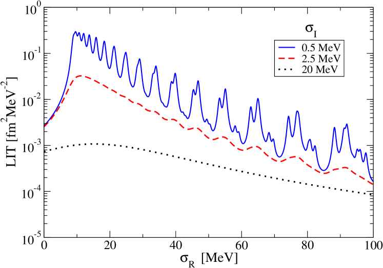
Figure 1: LIT of the ³He dipole response function for $T=1/2$ with $\sigma_{I}=0.5$, 2.5 and 20 MeV calculated with an HH basis of 30 hyperspherical and 31 hyperradial states for a total of 930 basis states ($b=0.3$ fm).

We start the discussion illustrating first results, where the HH basis is used for the calculation of the LIT of the ³He photodisintegration. We consider only the final state in the isospin $T=1/2$ channel, since the $T=3/2$ channel corresponds exclusively to a three-body breakup. In Fig. 1 we show results for various values of $\sigma_{I}$. One sees that with $\sigma_{I}=20$ MeV a smooth transform is obtained, then with an increase of the resolution to $\sigma_{I}=2.5$ MeV the transform starts to have an oscillating behaviour beyond 20 MeV, and a still further increase of the resolution to $\sigma_{I}=0.5$ MeV exhibits the underlying structure of the single LIT states (see Eq. (11)). From the last result one can conclude that the resolving power of the LIT is certainly not just given by the chosen $\sigma_{I}$ value.

For a higher degree of resolution one has to increase the density of LIT states, which can be achieved in two ways, namely by increasing the number of basis functions and by enhancing the $b$ parameter of the hyperradial wave function of Eq. (15). Both measures are taken for the results shown in Fig. 2, where we illustrate the low-energy part of the LIT for rather small $\sigma_{I}$ values. It is evident that the density of LIT states grows as expected. In Fig. 2d one observes a rather high LIT state density and one could easily further increase the density. However, one readily sees that there is not a single LIT state below the three-body breakup threshold at about 8 MeV (³He binding energy with MT-I/III potential). On the other hand the calculation of the $S$-factor $S_{12}$ requests energies just beyond the two-body breakup threshold at 5.8 MeV (difference of binding energies of ²H and ³He for the MT-I/III potential). Thus one cannot expect that an inversion of the LITs of Fig. 2 leads to a high-precision result in the region of astrophysical relevance. Here a comment is in order concerning the use of a more realistic nuclear force for a calculation of the LIT with the HH basis. In this case one can find a few LIT states below the three-body breakup threshold, but also there one encounters the problem of further increasing the density of LIT states in a systematic way in order to obtain a smooth LIT with a sufficiently small $\sigma_{I}$ BaB13 ; Lei15 .

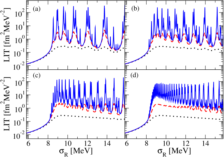
Figure 2: Low-energy part of the LIT of Fig. 1 with $\sigma_{I}=0.01$ (full), 0.1 (dashed) and 0.5 MeV (dotted), results with different HH basis systems: (a) same basis as in Fig. 1, (b) 40 hyperspherical and 51 hyperradial states ($b=0.3$ fm), (c) as in (b), but with $b=0.5$ fm, (d) 40 hyperspherical and 76 hyperradial states ($b=1$ fm).

Now we turn to the results with the Jacobi basis. Since in principle we are only interested in the cross section just above the two-body breakup threshold we only consider $S$-wave interaction for the pair coordinate, this means that in Eq. (12) only basis states with $l_{1}=0$ and $l_{2}=1$ are taken into account (as already mentioned for the dipole response we have $L=1$). For the radial parts of the pair and single-particle wave functions we choose $b_{1}=0.75$ fm and $b_{2}=0.5$ fm, respectively.

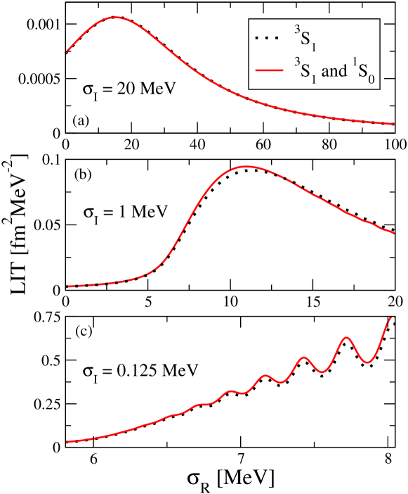
Figure 3: LIT of the ³He dipole response function for $T=1/2$ with $\sigma_{I}=20$, 1 and 0.125 MeV calculated with the Jacobi basis taking into account only ${}^{3}S_{1}$ states in the pair coordinate of $\phi$ (dotted) and in addition also ${}^{1}S_{0}$-states (full).

In Fig. 3 we show the LIT for the cases that the pair in $\phi$ of Eq. (16) is solely in a ${}^{3}S_{1}$-state and the additional effect when also ${}^{1}S_{0}$-states are allowed. One sees that the contribution due to the ${}^{1}S_{0}$-states is quite tiny. In fact a rather small number of basis states with the pair in the ${}^{1}S_{0}$ state ($N_{1}=5$, $N_{2}=19)$ is sufficient in order to obtain convergence. As shown in Fig. 4 the convergence of the main LIT contribution due to the ${}^{3}S_{1}$-states is not as rapid as in case of the ${}^{1}S_{0}$ states. On the one hand one needs only a rather moderate value for $N_{1}$ of about 20 to obtain a sufficient convergence in the pair coordinate as shown in Fig. 4b (note a result with $N_{1}$=24 could not be distinguished in the figure from the $N_{1}=19$ result). On the other hand the situation is different for the single-particle coordinate (see Fig. 4a). In order to have a sufficiently convergent LIT in the region just above the two-body breakup threshold with a small $\sigma_{I}$ value of 0.125 MeV one has to go up to an $N_{2}$ of about 70. In fact for our calculation of the $S$-factor $S_{12}$ we use $N_{2}=79$.

It is interesting to observe the different effects of an increase of $N_{1}$ and $N_{2}$. The enhancement of basis states for the pair coordinate in Fig. 4b shifts the transform to lower energies without changing the shape of the LIT. This corresponds to an energy shift of the low-energy LIT states to lower energies without a notable change of the density. On the contrary the increase of basis states for the single-particle coordinate (Fig. 4a) leads to a smoother result of the transform due to an increased density of LIT states.

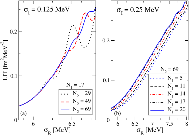
Figure 4: Convergence pattern for the LIT of the ³He dipole response function for $T=1/2$ calculated with the Jacobi basis: (a) $N_{1}=17$ and various $N_{2}$ values ($\sigma_{I}=0.125$ MeV) and (b) $N_{2}=69$ and various $N_{1}$ values ($\sigma_{I}=0.25$ MeV).

In Fig. 5 we compare the low-energy LIT calculated with HH and Jacobi basis systems for various $\sigma_{I}$ values. Note that different from the case with the Jacobi basis, where only $S$-wave interaction is taken into account, for the HH basis also interaction in higher partial waves is considered, however, the contribution of the latter should be quite small. In fact for large $\sigma_{I}$ (see Fig. 5a) one can hardly find any difference between both results. Even for $\sigma_{I}=5$ MeV, shown in Fig. 5b, the results are rather similar, whereas a decrease of $\sigma_{I}$ to 0.5 MeV, also shown in Fig. 5b, exhibits quite some difference: the peak of the LIT of the HH basis is considerably more pronounced than that of the Jacobi basis. To a large extent the difference is caused by the missing LIT states at low energy for the HH basis and not by the additional interaction in higher partial waves. Thus one may conclude that the lack of low-energy LIT states leads to a shift of low-energy strength to the peak region region just above the two-body breakup threshold.

The energy distribution of low-energy LIT states for both basis systems is nicely illustrated in Fig. 5c for $\sigma_{I}=0.01$ MeV. Only for the Jacobi basis one finds LIT states directly above the two-body breakup threshold. The LIT state density is so high that one obtains a smooth LIT in the very threshold region even with $\sigma_{I}=0.1$ MeV and up to the three-body breakup threshold with $\sigma_{I}=0.25$ MeV.

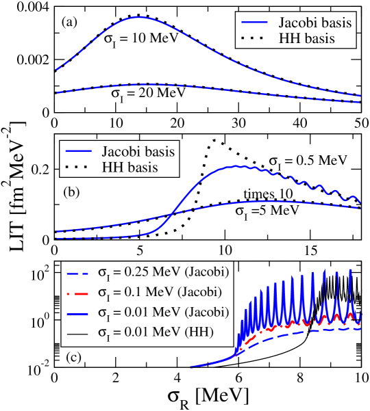
Figure 5: Comparison of the LIT calculated with HH and Jacobi basis systems with various $\sigma_{I}$ values as indicated in the figure.

In order to determine the cross section $\sigma_{\gamma}$ one has to invert the calculated transforms. With regard to the aim to determine the $S$-factor it is evident that close to the threshold region one wants to work with a high resolution, however, one has to take into account that with a small $\sigma_{I}$ value one does not obtain a smooth LIT at higher energies because the density of LIT states decreases with growing energy. In fact it is better to work with an energy dependent $\sigma_{I}$. Therefore we divide the $\sigma_{R}$ range in various intervals [$E_{j}$, $E_{j+1}]$ ($j=1,2,3,...,J)$ and take in this interval $\sigma_{I}=\sigma_{I,j}$. Considering that we have calculated the LIT for a certain number of $\sigma_{R}$ points $\sigma_{R,k}$ ($k=1,2,3,...,K)$ we rescale the LIT for all $\sigma_{R,k}\geq E_{j+1}$ by the factor

$$f(j+1)={\frac{L(\sigma_{k_{2}(j)},\sigma_{I,j})}{L(\sigma_{k_{1}(j+1)},\sigma_{I,j+1})}}\,,$$ (21)

where $\sigma_{k_{1}(j)}$ is the lowest and $\sigma_{k_{2}(j)}$ the highest $\sigma_{R}$ value in interval [$E_{j}$, $E_{j+1}]$. Note that this is made in a cumulative way, thus for the LIT in the last interval ($\sigma_{R}\in[E_{J-1}$, $E_{J}]$) we have the total factor $F=f(2)f(3)...f(J)$. The values we have chosen for $E_{j}$ and $\sigma_{I,j}$ are given in Table I. The application of Eq. (21) and the definitions given in Table 1 define a new transform ${\cal L}$.

Table 1: $E_{j}$ and $\sigma_{I,j}$ values for the definition of the new transform ${\cal L}$

$j$	$E_{j}$ [MeV]	$\sigma_{I,j}$ [MeV]
1	5.7	0.125
2	6.15	0.175
3	6.55	0.35
4	8.05	0.7
5	10.55	1.1
6	13.05	1.5
7	23.05	5
8	58.05	10
9	108.05	20
10	308.05	-

In Fig. 6 we show the newly defined transform ${\cal L}(\sigma)$, where we use a Jacobi basis with ($N_{1}=24$, $N_{2}=79)$ and ($N_{1}=5$, $N_{2}=19)$ for the ${}^{3}S_{1}$ states and the ${}^{1}S_{0}$ states, respectively. The dashed curve in the figure shows the LITs $L$ for the various energy intervals without any additional factor, whereas the continuous curve corresponds to the result when the additional factors of Eq. (21) are introduced. Note that according to the definition of the $f(j)$ the derivative of ${\cal L}$ seems to be not continuous, but actually this is not the case since the transform is only defined pointwise in $K$ $\sigma_{R}$ points. In principle one could also work with the transform described by the dashed curve in Fig. 6, but this would mean that the impact of the transform is reduced with growing energy. The rescaling simulates the case where the transform is calculated with a single $\sigma_{I}$.

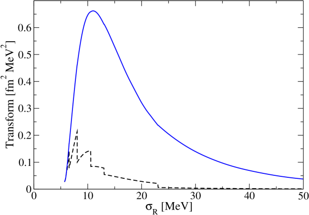
Figure 6: The LITs $L$ with $\sigma_{I}=\sigma_{I,j}$ in the various energy intervals $[E_{j}$, $E_{j+1}]$ (dashed) and the new transform ${\cal L}$ (full) as described in the text.

For the inversion we use our standard method, where the response function $R$ is expanded as follows

$$R(E_{\gamma}=E+E_{thr})=\sum_{n=1}^{N}c_{n}g_{n}(E)\,,$$ (22)

where $E$ is defined as in Eq. (1) and $E_{thr}$ is the energy of the two-body breakup threshold. In order to consider the effect of the Coulomb barrier we include the Gamow factor of Eq. (1) taking

$$g_{n}(E)=\exp(-2\pi\eta)\exp[(-\alpha E)/n]\,,$$ (23)

where $\alpha$ is a non-linear parameter. The various $g_{n}(E)$ are then transformed numerically to the $\sigma$-space according to the LIT transformation given in Eq. (6) for the response function. Note that in case of the transform ${\cal L}$ the factors $f(j)$ of Eq. (21) have to be taken properly into account. In this way one obtains a set of functions $\tilde{g}_{n}(\sigma)$ which are then used for the expansion of the transform, here given for the case of ${\cal L}$,

$${\cal L}(\sigma)=\sum_{n=1}^{N}c_{n}\tilde{g}_{n}(\sigma)\,.$$ (24)

For given values of $N$ and $\alpha$ of Eqs. (22) and (23) a best fit to the calculated ${\cal L}$ is made, which determines the coefficients $c_{n}$. Varying then only the non-linear parameter $\alpha$ over a wide range values one obtains the absolute best fit for a specific $N$. Then one repeats the procedure increasing $N$ by one. A stable inversion result should be obtained in a range $N_{A}\leq N\leq N_{B}$.

In Fig. 7 we show inversion results of $L(\sigma)$ for the HH basis and of ${\cal L}$ for the Jacobi basis. The parameters for the HH basis are the same as defined in caption of Fig. 2d, for the Jacobi basis we use the new transform ${\cal L}$ with the setting ($N_{1}=24$, $N_{2}=79$) and ($N_{1}=5$, $N_{2}=19$) for ${}^{3}S_{1}$- and ${}^{1}S_{0}$-states in the pair coordinate, respectively. Note that for the HH basis we take $\sigma_{I}=20$ MeV. We do not choose a higher resolution otherwise the inversion could be hampered too much by the fact that the low-energy strength is shifted to the peak region. Due to this misplaced strength one cannot expect that the two inversion results are extremely close to each other. On the other hand, as Fig. 7a shows, differences remain rather small. The peak heights are almost identical, but the peak of the HH basis is shifted somewhat to higher energies.

It is a bit surprising that the low-energy cross sections are not completely different (see Fig. 7b), but this is due to the correct implementation of the Gamow factor in the set of functions $g$ for the inversion. It is interesting to check the effect of an inversion of ${\cal L}$, where the Gamow factor in Eq. (23) is replaced by the factor $E^{3/2}$ (correct threshold behaviour without Coulomb barrier). Although we have a high-precision transform for the Jacobi basis the inversion without the Gamow factor does not lead to the correct threshold behaviour, but at least coincides with the proper inversion result above about 6 MeV.

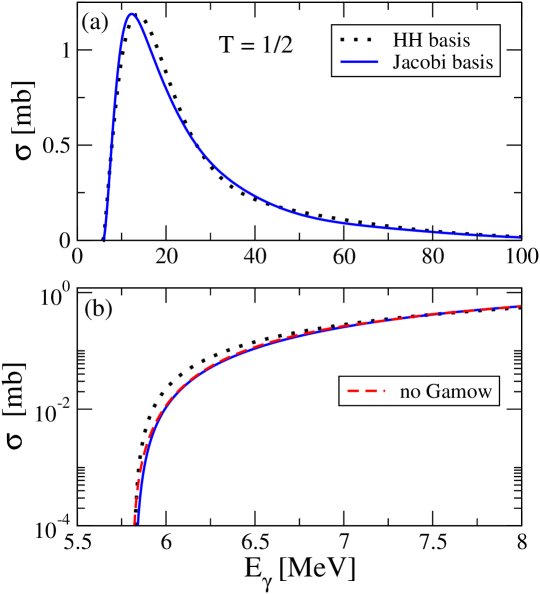
Figure 7: The ³He cross section $\sigma_{\gamma}$ of Eq. (4) obtained from inversions of $L(\sigma_{R},\sigma_{I}=20$ MeV) with HH basis (dotted) and of ${\cal L}(\sigma)$ with Jacobi basis (full); in (b) also shown inversion of ${\cal L}(\sigma)$ with Jacobi basis with factor $E^{3/2}$ instead of Gamow factor in functions $g$ of Eq. (23) (dashed).

In Fig. 8 we show a comparison of the LIT result with that of a calculation with explicit continuum wave functions. In the upper panel the ³He photodisintegration cross section $\sigma_{\gamma}$ is depicted. It is evident that there is an excellent agreement between both results. However, because of the strong fall-off of $\sigma_{\gamma}$ close to the breakup threshold it is difficult to understand the level of agreement in this energy range. This can be estimated much better for the $S$-factor since the Gamow factor is divided out. In Fig. 8b one finds also in this case a very good agreement between both calculations. It is worthwhile to mention that we find quite stable inversion results $11\leq N\leq 18$, where $N$ is the number of basis function used for the inversion (see Eqs. (22) and (23)). This enables us to make the following error estimate for the LIT inversion. We take the inversions for $N=11$ ($F_{\rm inv,11}(E)$) up to $N=18$ ($F_{\rm inv,18}(E)$) and first determined an average inversion result $\bar{F}_{\rm inv}(E)=\sum_{i=11}^{18}F_{\rm inv,i}(E)/8$, which is described by the full cure in Fig. 8b. In addition we have calculated the energy dependent standard deviation $\sigma_{\rm std}(E)$ and the dashed curves correspond to $\bar{F}_{\rm inv}(E)\pm\sigma_{\rm std}(E)$. As one sees the inversion error is rather small, but grows towards lower energies. One could further improve the inversions by making an even more precise LIT calculation. In our specific case it would probably be better to change the $b_{i}$ parameters of the radial basis function a bit rather than to increase the number of basis functions.

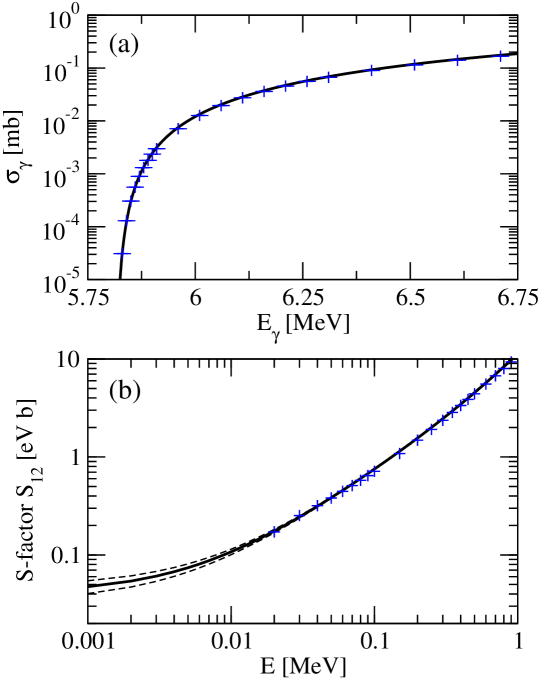
Figure 8: (a) Full curve same as in Fig. 7b and in addition results from the direct calculation with explicit continuum wave function (plus signs); (b) same results as in (a) but rescaled in order to determine the $S$-factor (see Eqs. (1) and (3)), inversion error shown by dashed lines (see text).

We summarize our work as follows. We have tested the LIT method for a calculation of the $S$-factor of the reaction ²H$(p,\gamma)^{3}$He using a simple central NN interaction (MT-I/III potential). The calculation is performed by first computing the cross section of the inverse reaction in unretarted dipole approximation and then using the law of detailed balances in order to determine the deuteron-proton capture cross section which then leads to the determination of the $S$-factor. For a precise application of the LIT method it is necessary to have a sufficient density of LIT states in the energy region of interest. Considering our specific case this corresponds for the ³He photodisintegration to the energy region between the two- and three-body breakup thresholds. We have found that a solution of the LIT equation with the MT-I/III potential via an expansion in hyperspherical harmonics does not yield a single LIT-state below the three-body breakup threshold, even though using a rather high number of basis functions of a rather large spatial extension. With a more realistic nuclear force the picture does not change essentially as can be deduced from another low-energy observable, namely the ⁴He isoscalar monopole resonance BaB13 ; Lei15 . As pointed out in Lei15 for an increase of the LIT state density in the low-energy region one needs to use a basis where the relevant dynamical variable, namely the single-particle coordinate (vector pointing from the center of mass of the (A-1) particle system to the A-th particle), appears explicitly. Therefore we have taken a basis which is a product of expansions of two basis systems, each of them depending either on the single-particle coordinate or on the pair coordinate. We could show that using such a basis one can systematically increase the low-energy LIT state density. Furthermore, we show that in order to take into account that the LIT states become less dense with increasing energy it is advantageous to use different $\sigma_{I}$-values in different energy intervals.

In addition to the LIT approach we have carried out the calculation with explicit contin- uum wave functions. They have been determined via solving the Schrödinger equation with the help of an expansion over a proper basis set. A comparison of results from both methods shows a very good agreement. For the LIT method we have also included an estimate of the inversion error.

References

- (1) E.G. Adelberger et al., Rev. Mod. Phys. 83, 195 (2011).
- (2) W. Leidemann and G. Orlandini, Prog. Part. Nucl. Phys. 68, 158 (2013).
- (3) J. Carbonell, A. Deltuva, A.C. Fonseca, and R. Lazauskas, Prog. Part. Nucl. Phys. 74, 55 (2014).
- (4) V.D. Efros, W. Leidemann and G. Orlandini, Phys. Lett. B 338, 130 (1994).
- (5) N. Barnea, V.D. Efros, W. Leidemann and G. Orlandini, Few-Body Syst. 47, 201 (2010).
- (6) D. Andreasi, W. Leidemann, Ch. Reiss and M. Schwamb, Eur. Phys. J. A, 24, 361 (2005).
- (7) W. Leidemann, Few-Body Syst. 42, 139 (2008).
- (8) V.D. Efros, W. Leidemann, G. Orlandini and N. Barnea, J. Phys. G 34, R459 (2007).
- (9) S. Bacca and S. Pastore, J. Phys. G 41, 123002 (2014).
- (10) S. Bacca, N. Barnea, W. Leidemann, and G. Orlandini, Phys. Rev. Lett. 110, 042503 (2013); Phys. Rev. C 91, 024303 (2015).
- (11) N. Barnea, W. Leidemann and G. Orlandini, Phys. Rev. C 61, 054001 (2000); Nucl. Phys. A 693, 565 (2001).
- (12) N. Barnea, V.D. Efros, W. Leidemann and G. Orlandini, Few-Body Syst. 35, 155 (2004).
- (13) W. Leidemann, Phys. Rev. C 91, 054001 (2015).
- (14) R.A. Malfliet and J.A. Tjon, Nucl. Phys. A 127, 161 (1969).
- (15) L.E. Marcucci, M. Viviani, R. Schiavilla, A. Kievsky and S. Rosati, Phys. Rev. C 72, 014001 (2005).
- (16) L.E. Marcucci, G. Mangano, A. Kievsky and M. Viviani, Phys. Rev. Lett. 116, 102501 (2016).
- (17) V. D. Efros, W. Leidemann and G. Orlandini, Phys. Lett. B 408, 1 (1997).
- (18) B.N. Zakhariev, V.V. Pustovalov and V.D. Efros, Sov. J. Nucl. Phys. 8, 234 (1968); V.P. Permjakov, V.V. Pustovalov, Yu.I. Fenin and V.D. Efros, Sov. J. Nucl. Phys. 14, 317 (1972).
- (19) C. Schwartz, Ann. Phys. 16, 36 (1961).
- (20) E.W. Schmid and K.H. Hoffmann, Nucl. Phys. A 175, 443 (1971).
- (21) A. Kievsky, priv. comm. (2016).
- (22) A. Deltuva, A.C. Fonseca, A. Kievsky, S. Rosati, P.U. Sauer, M. Viviani, Phys. Rev. C 71, 064003 (2005).
- (23) S. Deflorian, PhD thesis, University of Trento (2016).