Interferometric Monitoring of Gamma-ray Bright AGNs I: Results of Single-epoch Multifrequency Observations

Abstract

We present results of single-epoch very long baseline interferometry (VLBI) observations of gamma-ray bright active galactic nuclei (AGNs) using the Korean VLBI Network (KVN) at 22, 43, 86, and 129 GHz bands, which are part of a KVN key science program, Interferometric Monitoring of Gamma-ray Bright AGNs (iMOGABA). We selected a total of 34 radio-loud AGNs of which 30 sources are gamma-ray bright AGNs with flux densities of $>6\times 10^{-10}$ ph cm^-2 s^-1. Single-epoch multi-frequency VLBI observations of the target sources were conducted during a 24-hr session on 2013 November 19 and 20. All observed sources were detected and imaged at all frequency bands with or without a frequency phase transfer technique which enabled the imaging of 12 faint sources at 129 GHz, except for one source. Many of the target sources are resolved on milliarcsecond scales, yielding a core-jet structure with the VLBI core dominating the synchrotron emission on the milliarcsecond scale. CLEAN flux densities of the target sources are 0.43-28 Jy, 0.32-21 Jy, 0.18-11 Jy, and 0.35-8.0 Jy in the 22, 43, 86, and 129 GHz bands, respectively. Spectra of the target sources become steeper at higher frequency with the mean of the spectral indices of -0.40, -0.62, and -1.00 in the 22-43 GHz, 43-86 GHz and 86-129 GHz bands, respectively, implying that the target sources become optically thin at higher frequency (e.g., 86-129GHz).

1 Introduction

Active galactic nuclei (AGNs) are the most powerful and violent celestial objects in the Universe. AGNs emit a wide range of electromagnetic radiation in the radio to gamma-ray range, producing huge luminosity ($\sim 10^{42}-10^{48}$ erg s^-1) in very compact emitting regions on sub-pc scales; their emission is often highly variable and polarized (see e.g., Krolik, 1999). The AGNs are believed to have supermassive black holes (SMBH) in the centers, accretion disks around the SMBHs, and relativistic jets launched perpendicular to the accretion disk plane into interstellar space. Relativistic jets of the radio-loud AGNs often show variability in brightness (e.g., in radio, optical, etc.) on timescales of hours to years, and morphological changes on milliarcsecond (mas) scale (see e.g., Boettcher et al., 2012, for review).

Very rapid and strong variabilities (or flares) in the gamma-ray range from radio-loud AGNs have been observed during intensive gamma-ray monitoring of AGNs by several gamma-ray space telescopes: INTEGRAL , AGILE , FERMI , etc. The gamma-ray flares were detected from more than 100 AGNs including 3C 273, 4C +21.35, 4C 454.3 and 1510-089, by the Fermi Gamma-ray Space Telescope (GST) (see Kang et al., 2015, for references). To understand the gamma-ray flares in the AGNs, multiwavelength monitoring studies have been conducted to investigate the correlation between emission at gamma-ray and other wavelengths (e.g., Marscher et al., 2008; Abdo et al., 2010). The gamma-ray flares are correlated with the variability in brightness, polarization, and morphology of the jets at low energy regimes (e.g., radio, optical, etc.). The correlation of the gamma-ray flares with multiwavelength variability, in principle, implies co-spatiality of the gamma-ray flaring regions and the emission regions at other wavelengths.

Marscher et al. (2008) suggested that the gamma-ray flares from BL Lac may be generated through inverse Compton scattering in the innermost region of the jets threaded by a helical magnetic field or in a bright very long baseline interferometry (VLBI) core region corresponding to a standing shock wave, through compression by the shock front. Abdo et al. (2010) reported that the gamma-ray flares correlated with the change of optical polarization angle of 3C 279 provide evidence for the co-spatiality of the gamma-ray and optical emission regions with a highly ordered jet magnetic field in a curved trajectory within the jet. The different understandings of the cause and location of the gamma-ray flares imply that either the gamma-ray flares are generated under various situations or our understanding of the gamma-ray flares may still be uncertain.

Gamma-ray flares leading a delayed outburst at radio frequencies (e.g., Jorstad et al., 2001) motivated the conducting of many single-dish and VLBI observations (or monitoring programs) at centimeter (cm) and millimeter (mm) wavelengths (Savolainen et al., 2002; Lähteenmäki & Valtaoja, 2003; Lister et al., 2009; Ojha et al., 2009; Marscher et al., 2011; Angelakis et al., 2012; Nagai et al., 2013). Those VLBI monitoring programs are conducted only at a single frequency of $\leq$43 GHz, except for the TANAMI (Ojha et al., 2009) at 8.4 and 22 GHz, implying that those programs are not able to determine frequency-dependent properties of the gamma-ray flaring AGNs on mas-scales, including such properties as spectral index variation, time-dependent multiwavelength light curves of mas-scale structures, etc., which may be very important to investigate the correlation of the gamma-ray flares with both the optically thin and thick emissions of the jets.

The Korean VLBI Network (KVN) has enabled us to regularly obtain mas-scale images of gamma-ray bright AGNs at cm-to-mm wavelengths, leading to a key science program (KSP) of the KVN, the Interferometric Monitoring of Gamma-ray Bright AGNs (iMOGABA), which is a VLBI monitoring program for about 30 gamma-ray bright AGNs using the KVN at multifrequency bands (22-129 GHz). The iMOGABA initially started in 2012 December by conducting monthly one 24-hr VLBI observation in the 22, 43, 86, and 129 GHz bands. The iMOGABA has been selected as a KVN KSP since 2015 March, aiming at studying the origins of the gamma-ray flares of the AGNs. We selected a total of 34 radio-loud AGNs, as summarized in Table 1, of which 30 sources are gamma-ray bright AGNs with their flux densities of $>6\times 10^{-10}$ ph cm^-2 s^-1, including 24 sources monitored by the Fermi Gamma-ray Space Telescope using the Large Area Telescope on board. The selected sources consist of 24 quasars, 7 BL Lacs, and 3 radio galaxies.

In this paper, the first representative paper from the iMOGABA program, we report the results of a single-epoch VLBI observations of the iMOGABA. In Section 2, the observations and data analysis of the single-epoch VLBI session used in this paper is described. Then, we present the results of the single-epoch observations in Section 3; in Section 4, we present our discussion. Finally, in Section 5, we summarize what we have found.

2 Observations and data analysis

2.1 Observations

We observed a total of 34 radio-loud AGNs in the 22 GHz, 43 GHz, 86 GHz, and 129 GHz bands on 2013 November 19 UT 02:00 - November 20 UT 01:53, using the KVN which consists of three identical 21-m radio telescopes (Lee et al., 2011): KVN Yonsei (KY), KVN Ulsan (KU), and KVN Tamna (KT), with baseline lengths of 305–476 km (Lee et al., 2014), and a simultaneous multifrequency observing system (Han et al., 2008, 2013). All sources were observed with 1-8 scans of 5 min in length. The observing frequencies were 21.700–21.764 GHz, 43.400–43.464 GHz, 86.800–86.864 GHz, and 129.300–129.364 GHz, and in left circular polarization (LCP). The ratio of the starting frequencies is an integer so that the frequency phase technique can be applied to faint sources (Algaba et al., 2015). The total bandwidth is 256 MHz and is divided evenly for each frequency band. In order to measure changes in the opacity of the atmosphere during the observations, we conducted sky tipping curve measurements every hour, i.e., we measured the system temperatures at 8 elevations: 18.21^∘, 20.17^∘, 22.62^∘, 25.77^∘, 30.00^∘, 36.03^∘, 45.58^∘, and 65.38^∘, during the observations. Cross-scan observations for target sources were conducted every scan to correct antenna pointing offsets, which are the main source of amplitude uncertainty in KVN observations. The received signals were digitized (i.e. 2-bit quantized) by digital samplers in the antenna cabin and transmitted through optical fibers to the observing building. The transferred digital signals were requantized and divided into 16 sub-bands (IFs) of 16 MHz wide by a digital filter bank, and recorded by the Mark 5B system at a recording rate of 1024 Mbps. Correlation of the data was performed with the DiFX software correlator in the Korea-Japan Correlator Center (Lee et al., 2015a).

2.2 Data analysis

The DiFX correlator produced the spectrum of the cross-correlation function with resolution of 0.125 MHz and accumulation period of 1 s. Post-correlation processing was done using the NRAO Astronomical Image Processing System (AIPS). A standard AIPS procedure was applied. An antenna-based fringe fitting was conducted using AIPS task FRING. KVN Ulsan (KU) was selected as the reference antenna. The 5 min long scans were split into solution intervals that were 30 s long. Baseline-based fringe solutions (phase delays and delay rates) were searched for individual IF at all frequency bands. The baseline-based fringe solutions were used to determine the antenna-based fringe solutions.

All sources were detected at lower frequencies (e.g., 22-86 GHz) with this standard post-correlation processing. However, about a dozen of the observed sources were not detected in the 129 GHz band. In order to detect the non-detected sources, the FPT technique was applied, using an automatic VLBI data reduction pipeline developed for the KVN observations. The operation of the KVN Pipeline was described in detail by Hodgson et al. (2016). Thanks to the FPT technique, i.e., by transferring phase solutions from lower frequencies to higher as described by Rioja & Dodson (2011) and Rioja et al. (2014), sensitivity at high frequency was improved, and all of the non-detected sources were detected in the 129 GHz band.

Amplitude calibrations were performed based on system temperatures measured during observations at each station and on elevation dependence of the antenna gains provided. The system temperatures were corrected for the atmospheric opacity estimated from the sky tipping curve measurements conducted every hour. We expect that thanks to the good quality of the system temperatures, antenna gains, and atmospheric opacity for KVN stations, the uncertainty of the amplitude calibration is witin 10-30% at 22-129 GHz bands. Re-normalization of the fringe amplitudes was made to correct for the amplitude distortion due to quantization, and the quantization and re-quantization losses were corrected (Lee et al., 2015b).

2.3 Imaging with calibrated data

The phase- and amplitude-calibrated data were used to produce CLEAN contour maps of the sources via the Caltech DIFMAP software (Shepherd et al., 1994). The calibrated data were averaged in frequency, and the data at band edges were chopped to avoid flux loss due to bandpass shape. The uv-data were also averaged in time over 30 seconds in the 22, 43, and 86 GHz bands, and over 10 seconds in the 129 GHz band, taking into account coherence time at each frequency bands, and expecting a decoherence loss of upto 30% at 86-129GHz bands. Some outliers in the $uv$-data were flagged by investigating the visibility amplitude.

The averaged and edited uv-data were then fitted using a single circular two-dimensional Gaussian model, and the visibility phase was self-calibrated with the model. After removing the single Gaussian model, a combination of CLEAN point source models was applied. The visibility phase was again self-calibrated with the CLEAN model to produce the final CLEAN contour maps of the detected sources, when available. The visibility amplitude was not modified.

The residual noise in the final CLEAN map was investigated to evaluate the quality of the image, taking into account the assumption that the residual noise of the properly CLEAN image is random noise, and hence the amplitude of each pixel in the residual map should have a Gaussian distribution. So, the noise in the final image can be expressed quantitatively by the ratio of image noise rms to its mathematical expectation, $\xi_{\rm r}=s_{\rm r}/s_{\rm{r,exp}}$, where $|s_{\rm r}|$ is the maximum absolute flux density in the residual image and $|s_{\rm r,exp}|$ is the expectation of $s_{\rm r}$. For Gaussian noise with a zero mean, the expectation of $s_{\rm r}$ is $|s_{\rm{r,exp}}|=\sigma_{\rm r}{\left[\sqrt{2}\ln{\left(\frac{N_{\rm pix}}{\sqrt{2\pi}\sigma_{\rm r}}\right)}\right]}^{1/2}$, where $N_{\rm pix}$ is the total number of pixels in the image, and $\sigma_{\rm r}$ is the image noise rms. If $\xi_{\rm r}\rightarrow 1$, the residual noise approaches Gaussian noise; if $\xi_{\rm r}>1$, not all the structure has been adequately recovered; if $\xi_{\rm r}<1$, the image model has an excessively large number of degrees of freedom (Lobanov et al., 2006). The values of $\xi_{\rm r}$ of the images obtained in this paper are 0.42-0.74 at 22 GHz, 0.41-0.77 at 43 GHz, 0.43-0.75 at 86 GHz, and 0.43-0.81 at 129 GHz, as shown in Figure 1 and summarized in Table 2, implying that the images adequately represent the structure detected in the visibility data.

2.4 Model fitting and estimating parameters

Circular two-dimensional Gaussian models were used to fit the final CLEAN images, yielding the general fit parameters: $S_{\rm tot}$ (total flux density), $S_{\rm peak}$ (peak flux density), $\sigma_{\rm rms}$ (post-fit rms), $d$ (size), $r$ (radial distance, for jet components), $\theta$ (position angle, measured for jet components, with respect to the location of the core component), as summarized in Table 3. The uncertainties of the fit parameters were estimated, based on the signal-to-noise ratio of each component detection, by adopting an analytical first order approximation given by Fomalont (1999): $\sigma_{\rm peak}=\sigma_{\rm rms}{\left({1+\frac{S_{\rm peak}}{\sigma_{\rm rms}}}\right)}^{1/2}$, $\sigma_{\rm tot}=\sigma_{\rm peak}{\left({1+\frac{S_{\rm tot}^{2}}{S_{\rm peak}^{2}}}\right)}^{1/2}$, $\sigma_{d}=d\frac{\sigma_{\rm peak}}{S_{\rm peak}}$, $\sigma_{r}=\frac{1}{2}\sigma_{d}$, and $\sigma_{\theta}={\rm atan}\left(\frac{\sigma_{r}}{r}\right)$, where $\sigma_{\rm peak}$, $\sigma_{\rm tot}$, $\sigma_{\rm rms}$, $\sigma_{d}$, $\sigma_{r}$, and $\sigma_{\theta}$ are the uncertainties of peak flux density, total flux density, post-fit rms, size, radial distance, and position angle of a component, respectively. A component was considered to be unresolved when the fitted component size $d$ is smaller than its minimum resolvable size (Lobanov, 2005) as given by $d_{\rm min}=\frac{2^{1+\beta/2}}{\pi}{\left[{\pi ab\ln 2\ln{\frac{\rm S/N}{{\rm S/N}-1}}}\right]}^{1/2}$, where a and b are the axes of the restoring beam, S/N is the signal-to-noise ratio, and $\beta$ is the weighting function, which is 0 for natural weighting or 2 for uniform weighting. If $d<d_{\rm min}$, the uncertainties were estimated according to $d=d_{\rm min}$.

The total flux density and measured size of a Gaussian component leads to a simple estimation of the rest frame brightness temperature $T_{\rm b}$ of the given emission region represented by the Gaussian model as $T_{\rm b}=\frac{2\ln{2}}{{\pi}{k}}\frac{S_{\rm tot}\lambda^{2}}{d^{2}}(1+z)$, where $\lambda$ is the wavelength of observation, $z$ is the redshift, and $k$ is the Boltzmann constant. If $d<d_{\rm min}$, then the lower limit of $T_{\rm b}$ is obtained using $d=d_{\rm min}$.

3 Results

Out of 34 sources, 32 sources were detected and imaged at all frequency bands with or without a frequency phase transfer technique that enabled us to detect and image 13 faint sources at 129 GHz, except for 0218+357 which was detected for only one baseline at all frequency bands. The first 129 GHz VLBI images were made for most of the sources in this project.

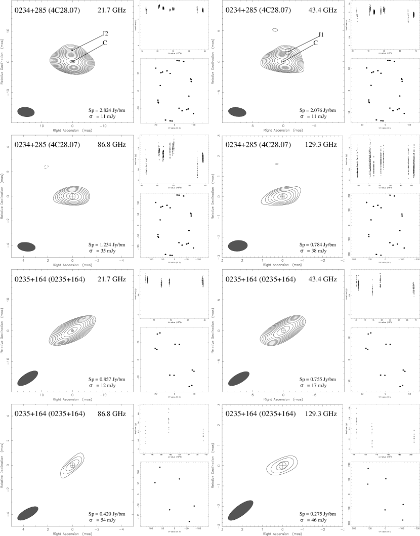
Figure 2: Contour maps of all sources with the distributions of the uv-sampling and of the visibility amplitude against uv-radius. In the left panel, a contour map of the CLEANed image is shown. The axes of the maps show the relative offset from the center of image in mas. Minimum contour level is shown in the lower-right corner of each map. The contours have a logarithmic spacing and are drawn at -1, 1, 1.4,…,$1.4^{n}$ of the minimum contour level. In the upper right panel, the X-axis represents the visibility amplitude (correlated flux density) in Jy, and the Y-axis shows the uv-distance in $10^{6}\lambda$. The corresponding uv-sampling distribution is given in the lower right palen. Image parameters of each image are summarized in Table 2.

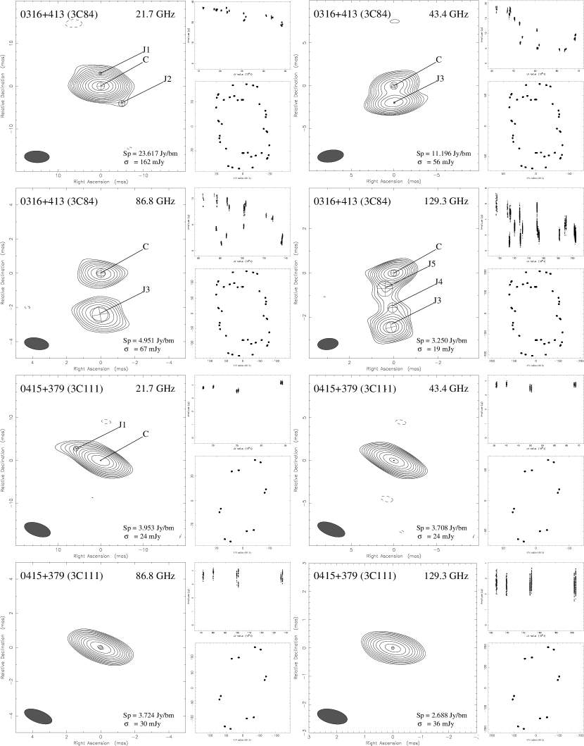
Figure 2: CLEAN images (continued)

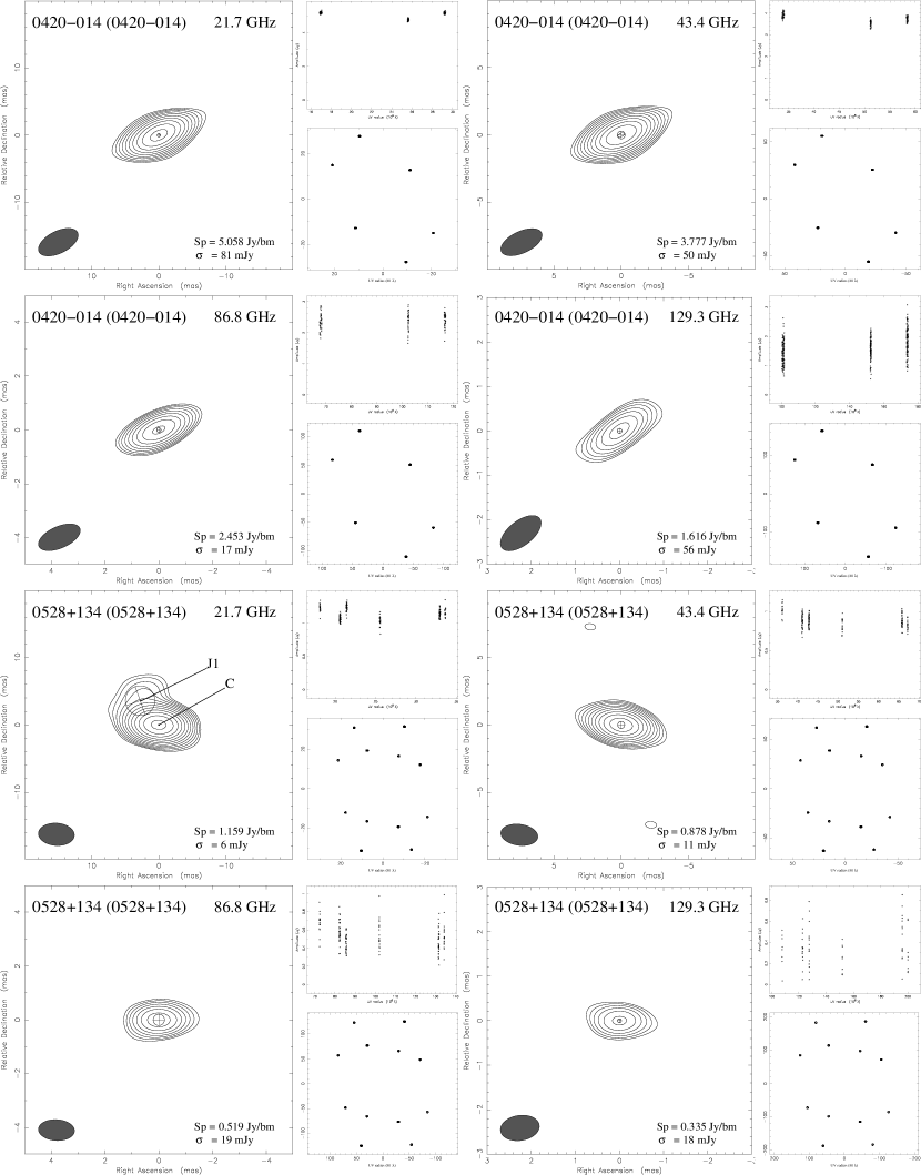
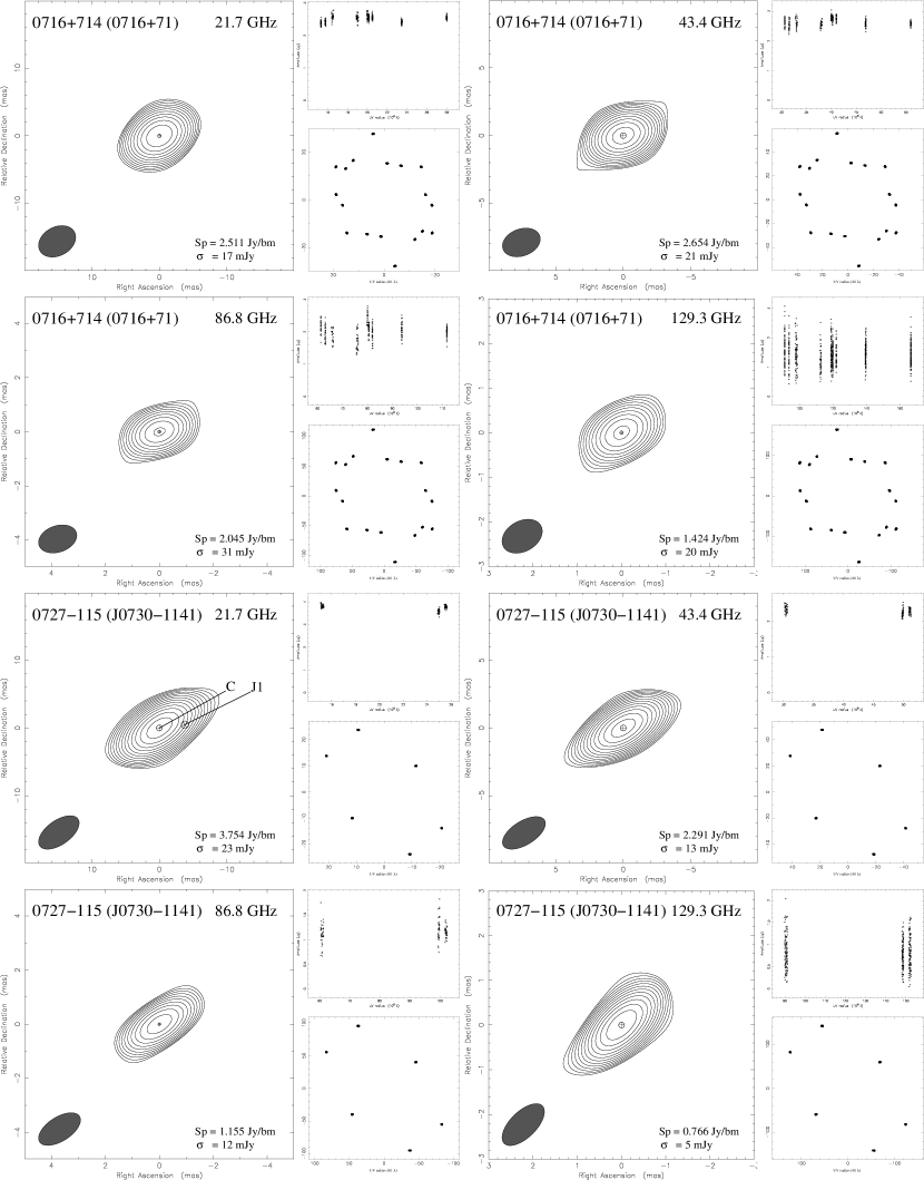
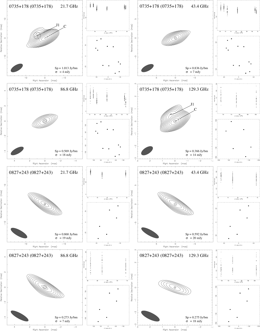
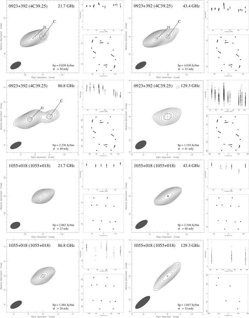
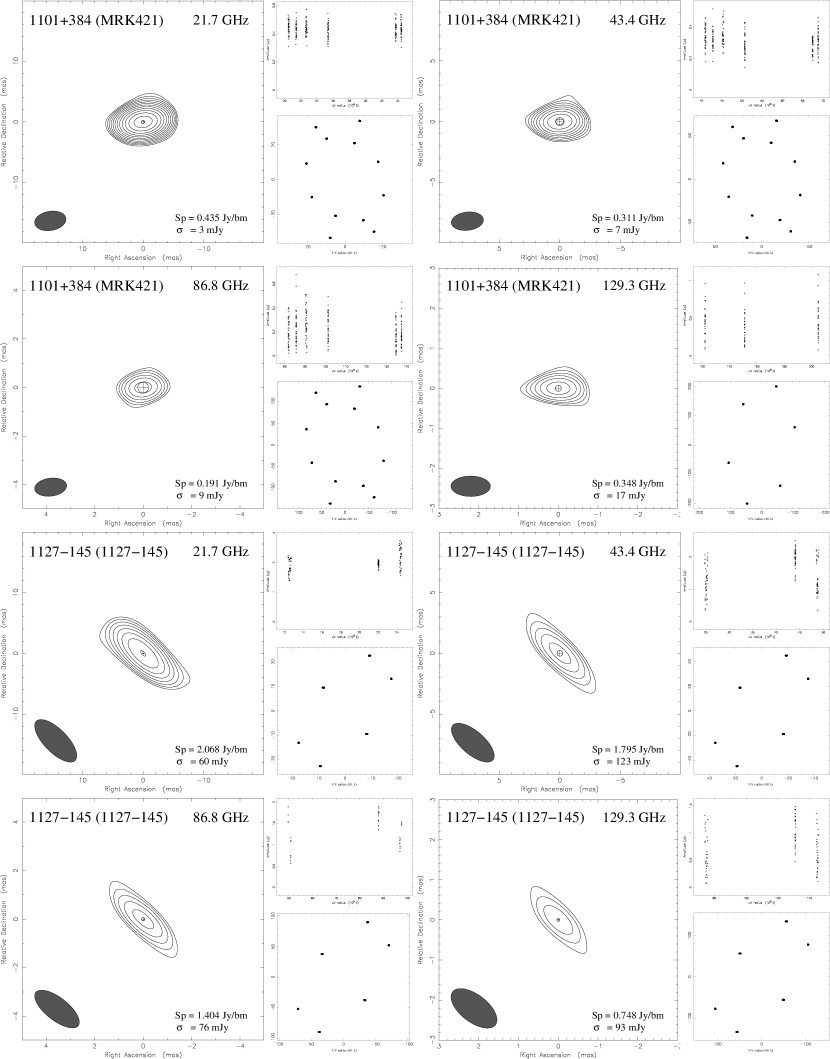
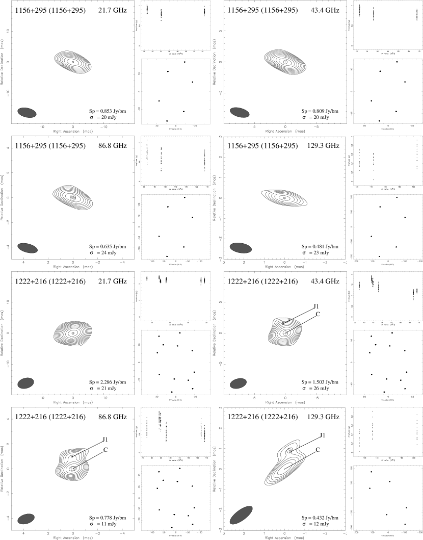
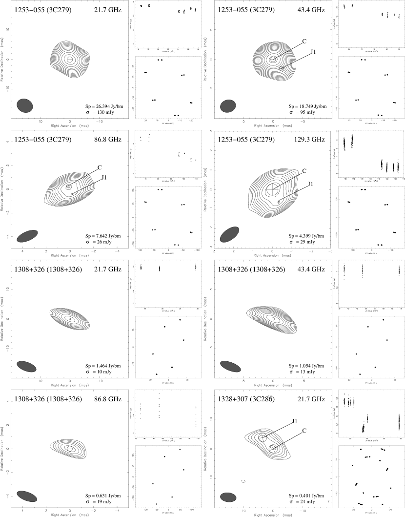
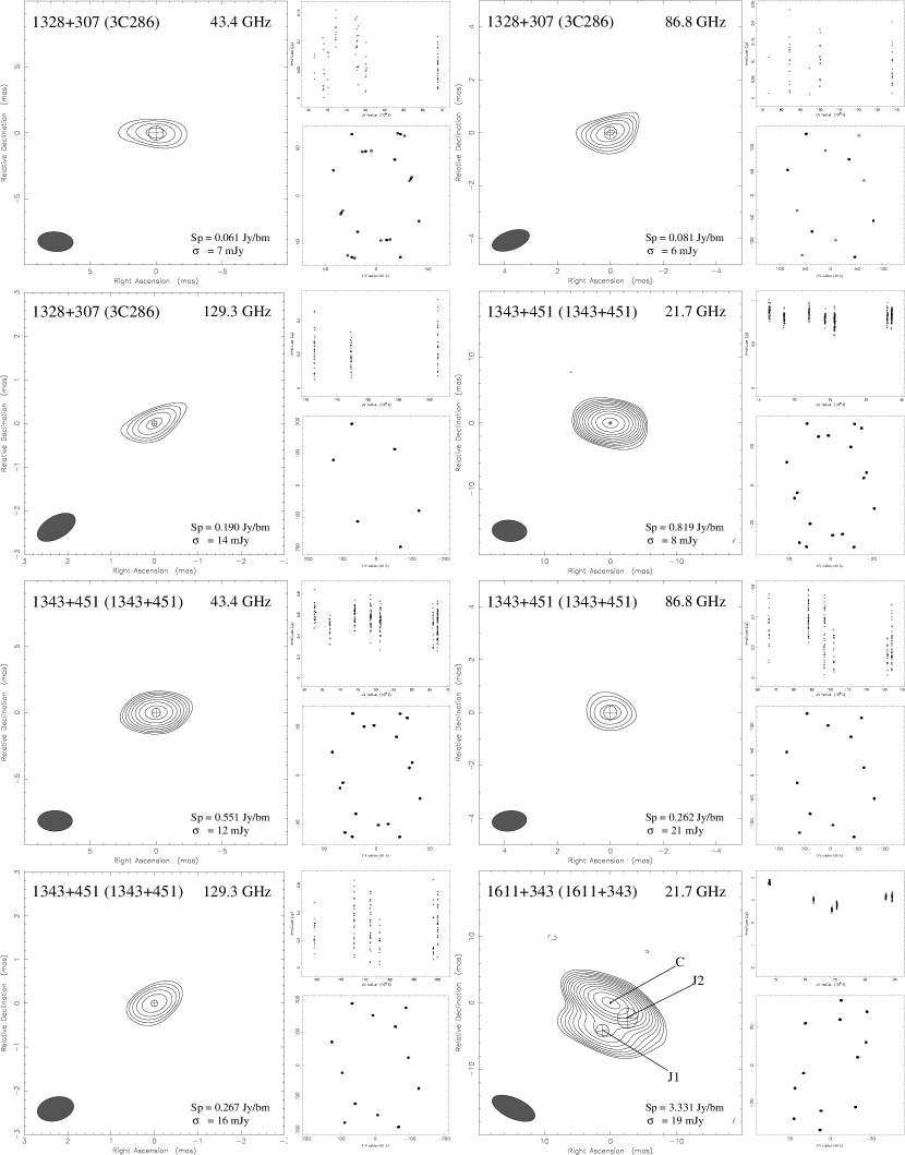
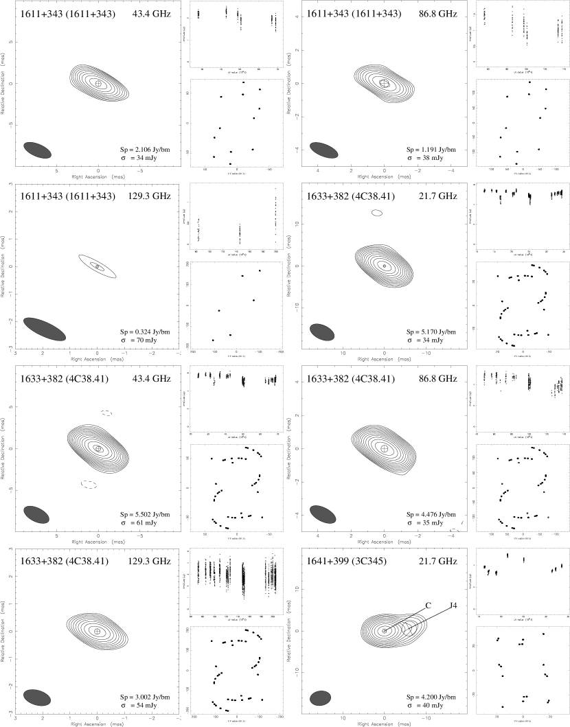
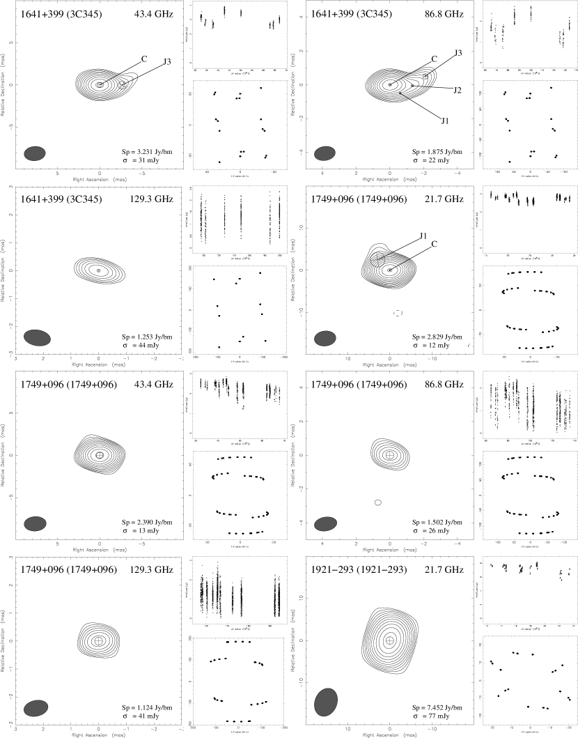
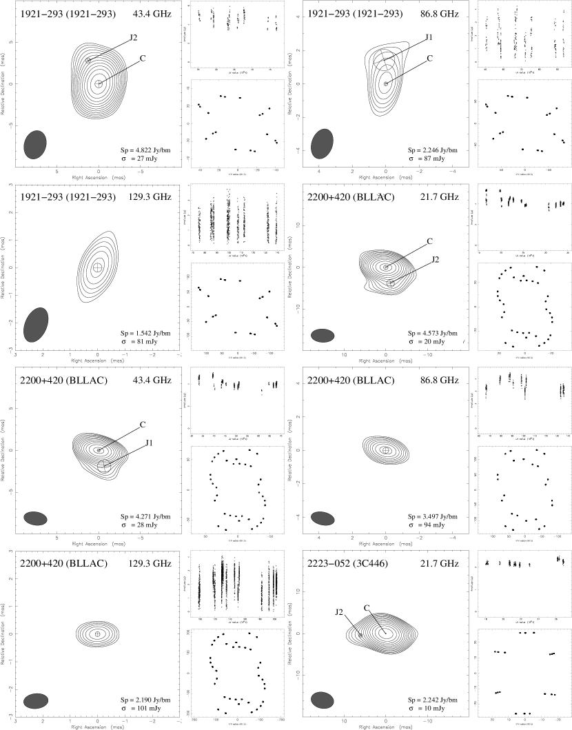
Figure 2: CLEAN images (continued)

Figure 2: CLEAN images (continued)

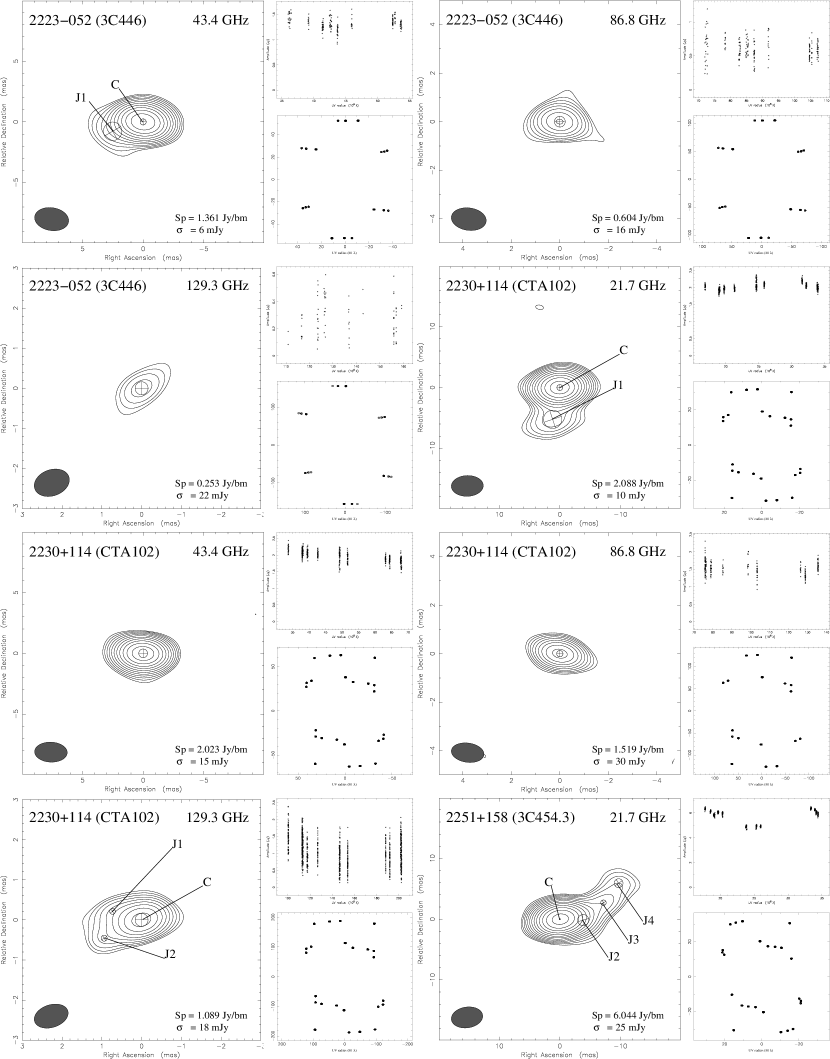
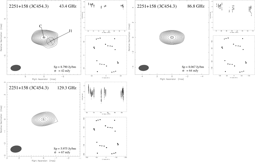
Figure 2: CLEAN images (continued)

In Figure 2, CLEAN contour maps for each source are presented for the 22, 43, 86, and 129 GHz bands, when available. A set of plots for each source at each frequency consists of a contour map in the left panel, a plot of the corresponding visibility amplitude against uv-radius in the top right panel, and a plot of the corresponding uv-sampling distribution in the bottom right panel. The contour map is shown with the X- and Y-axes in units of mas. The source name and the observing frequency are given at the top of the map. The FWHM of the restoring beam is drawn as a shaded ellipse on the map. The peak flux density and rms noise level are identified in the lower right corner of the map. The contours are drawn with a logarithmic spacing at -1, 1, 1.4,…,$1.4^{n}$ of the lowest flux density level which corresponds to three times the rms noise level. Most contour maps are centered on their brightest emission region (which is considered to be a VLBI core with fainter emission regions being the corresponding jet component, except for 3C 84 and 4C+39.25), but for some maps with extended source structure, the map center is shifted to fit the map in the box. The plot of the visibility amplitude, at the top right of each set, is drawn as a function of the uv-radius, i.e., the length of the baseline used to obtain the corresponding visibility point in units of $10^{6}\lambda$, where $\lambda$ is the observing wavelength. The visibility amplitude (i.e., the correlated flux density) is shown in units of Jy. The uv-sampling distribution, at the bottom right of each set, shows the distribution of the visibility in the uv-plane, whose range corresponds to that of the uv-radius. For the 12 sources (0235+164, 0528+134, 0735+178, 0827+243, 0836+710, 1127-145, 1156+295, 1222+216, 1343+451, 1611+343, and 3C 286) the FPTed images, i.e., the images obtained by the FPT technique, are presented for the 129 GHz band. In particular, the 43 and 86 GHz images for 3C 286 are also FPTed.

The KVN observations for this paper were done without the phase-referencing technique, i.e., without relative (or absolute) astrometric information of core or jet components with respect to calibrators. So, we considered a brightest emission region to be a VLBI core in each image and the others the jet, following a general strategy for identifying VLBI cores. However, we found that for some cases, maybe rare but well-known, the brightest component may not be the core. For example, 3C 84 (0316+413), the J3 component is brighter than the core (C) at 43 and 86 GHz. At 43 GHz, in particular, the J3 component was centered and the core was located in the northern area in the beginning of the imaging process due to its brightness. Considering the spectral index of the core (C) to be flat, we identified the northern component as a core, and shifted the map to south. Another exceptional source is 4C $+$39.25 (0923+392). The eastern component (J1) is brighter than the western component (C) and was located in the map center in the imaging process. Since, however, the fainter component is usually identified as the core (e.g., Niinuma et al., 2014), we considered the fainter component as the core and shifted the map to have the core in the center.

Parameters of the contour maps presented in Figure 2 are summarized in Table 2. For each image, Table 2 lists the source name, the observing frequency band, the parameters of the restoring beam (the size of the major axis $B_{\rm maj}$, the minor axis $B_{\rm min}$, and the position angle of the beam $B_{\rm PA}$), the total flux $S_{\rm KVN}$, the peak flux density $S_{\rm p}$, the off-source RMS $\sigma$, the dynamic range of the image $D$, and the quality $\xi_{\rm r}$ of the residual noise in the image.

The parameters of each model-fit component are listed in Table 3: the total flux $S_{\rm tot}$, peak flux density $S_{\rm peak}$, size $d$, radius, $r$ (only for jet components), position angle $\theta$ (only for jet components), and measured brightness temperature $T_{\rm b}$. In cases of multiple components (i.e., VLBI core and jet components) fitted, the parameters of the core component are followed by those of the jet components. The estimated uncertainties are given as in Section 2.4. The upper limits of size $d$, and the lower limits of brightness temperature $T_{\rm b}$ are in italics with flag symbols.

4 Discussion

4.1 Source morphology on mas scales

Many of the target sources are resolved on mas scales, yielding a core-jet structure. Out of 33 sources imaged, 22 sources show a core-jet structure at at least one of the observing frequency bands. Most of the sources with core-jet structure are imaged to show a single jet component, except for 0316+413 (3C 84), 1226+023 (3C 273B), 1611+343, 1641+399 (3C 345), 2230+114 (CTA102), and 2251+158 (3C 454.3), which show more than one jet component at at least one frequency band on the scales of 1-11 mas, contributing to the CLEAN flux density of the sources by $<$50%, as summarized in Table 3. Although many of the target sources are resolved, they are highly core-dominated in flux, i.e., the VLBI core flux density ($S_{\rm c}$) dominates the synchrotron emission on the mas-scales ($S_{\rm KVN}$), as shown in Figure 3. Some of the very compact sources show a ratio of $S_{\rm c}/S_{\rm KVN}$ larger than unity due to uncertainty of the CLEAN flux and of the model fitting.

The distributions of angular size for the core components of the imaged sources were investigated. As introduced in Section 2.4, a core component was considered to be unresolved when the fitted core size was smaller than its minimum resolvable size, yielding the upper limit of the angular size. The numbers of unresolved cores are 14 (22 GHz), 3 (43 GHz), 4 (86 GHz), and 5 (129 GHz) out of 33 imaged sources. Excluding the upper limits, the mean (and median) values of the measured core angular sizes are 1.135 mas (0.912 mas), 0.586 mas (0.591 mas), 0.411 mas (0.438 mas), and 0.232 mas (0.179 mas) in the 22, 43, 86, and 129 GHz bands, respectively, implying that the resolved core sizes become smaller at higher frequencies.

4.2 Brightness temperature

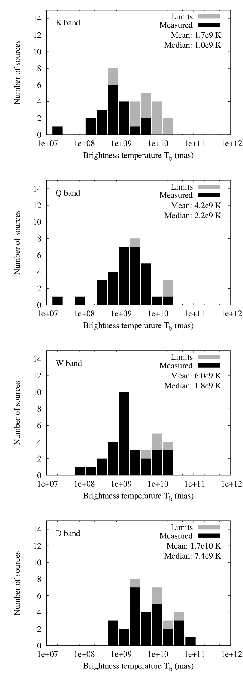
Figure 4: Distributions of the brightness temperature of the core components for the imaged sources. The mean and median of the distributions for the measured sizes are presented.

Figure 4 shows the brightness temperatures of the VLBI cores, including the lower limits (in grey), which were obtained for the unresolved cores (see Section 2.4). Excluding the limits, the measured brightness temperatures are in the ranges of $2.1\times 10^{7}$ K - $7.5\times 10^{8}$ K, $2.1\times 10^{7}$ K - $3.8\times 10^{10}$ K, $1.4\times 10^{8}$ K - $3.2\times 10^{10}$ K, and $7.7\times 10^{8}$ K - $1.2\times 10^{11}$ K, at 22, 43, 86, and 129 GHz, respectively. The mean values of the measured brightness temperature are $1.7\times 10^{9}$ K, $4.2\times 10^{9}$ K, $6.0\times 10^{9}$ K, and $1.7\times 10^{10}$ K in the 22, 43, 86, and 129 GHz bands, respectively, implying that the brightness temperatures of the sources become higher at higher frequency.

These results are different from those reported by Lee (2013), Lee (2014), and Lee et al. (2016): the brightness temperatures of the VLBI cores imaged at 86 GHz with the Global Millimeter VLBI Array (GMVA) are lower than those obtained at 2-15 GHz with the global VLBI array. The mean values of the brightness temperatures for the VLBI cores in Lee et al. (2016) are $8.9\times 10^{11}$ K and $1.3\times 10^{11}$ K at 15 and 86 GHz, respectively; these values are higher than those we obtained in this work, by factors of about 50 and 20, respectively, although the source samples and their sizes are different from each other. This difference may be due to the spatial resolution difference between the global VLBI arrays, which have a maximum baseline of about 10000 km, and the KVN, with its maximum baseline of about 500 km. However, the lower brightness temperatures at lower frequencies (e.g., 22 GHz) obtained with the KVN cannot be fully explained by the resolution difference. One explanation may be that the sources resolved at 22 GHz with the KVN are largely different from those resolved with the global array, since half of the cores in our sample were unresolved. Another explanation may be that the brightness temperature measurements at lower frequencies are affected partly by an instrumental beam blending effect: the core region may be diluted by jet emission (see e.g., Lee et al., 2016, and references therein). The core blending effect would make larger both the observed core flux density and the size. In this case of the 22 GHz observations with the KVN, the increasing factor of the observed core size $d$ is much larger than that of the observed core flux density $S_{\rm tot}$, and hence the brightness temperature ($\propto S_{\rm tot}/d^{2}$) becomes lower than its true value.

4.3 Source spectra

The 129 GHz images presented in this paper are the first results for most of the radio loud AGNs in our sample. Moreover, the simultaneous multifrequency images obtained at four frequency bands (22-129 GHz) are also the first results for the radio-loud AGNs, enabling us to investigate mas-scale spectral information for the radio loud AGNs free from any variability of source. Here we discuss the spectral properties of the target sources, taking into account the CLEAN flux densities obtained on mas-scales.

The CLEAN flux densities $S_{\rm KVN}$ of the target sources obtained with the KVN are in the ranges of 0.43-28 Jy, 0.32-21 Jy, 0.18-11 Jy, and 0.35-8.0 Jy in the 22, 43, 86, and 129 GHz bands, respectively, as shown in Figure 5. The distributions of the CLEAN flux density peak at around 2 Jy (22 and 43 GHz bands) and 1 Jy (86 and 129 GHz bands); these values show that most of the sources are brighter than 0.1 Jy at all frequencies. The mean values of the CLEAN flux density are 4.7 Jy (21.7 GHz), 3.8 Jy (43.4 GHz), 2.5 Jy (86.8 GHz), and 1.6 Jy (129.3 GHz), implying that the sources become fainter at higher frequency on mas-scales.

To investigate the spectral properties of the target sources, three models were used to fit it to the CLEAN flux density data: the power law, the broken power law, and the curved power law, as given by

$$S=a\nu^{\alpha},$$ (1)

where $S$ is the CLEAN flux density in Jansky, $\nu$ is the observing frequency in GHz, $a$ is constant in Jansky, and $\alpha$ is the spectral index for the power law,

$$S=b\left\{\left(\frac{\nu}{\nu_{\rm c}}\right)^{-\alpha_{\rm L}n}+\left(\frac{\nu}{\nu_{\rm c}}\right)^{-\alpha_{\rm H}n}\right\}^{-1/n},$$ (2)

where $b$ is constant in Jansky, $\nu_{\rm c}$ is a break frequency of the broken power law, $\alpha_{\rm L}$ and $\alpha_{\rm H}$ are the spectral indices at lower and higher frequencies than the break frequency, and $n$ is a numerical factor governing the sharpness of the break, here fixed to be 100 in order to make the break very sharp; and,

$$S=c_{1}\left(\frac{\nu}{\nu_{\rm r}}\right)^{\alpha+c_{2}{\rm ln}(\nu/\nu_{\rm r})},$$ (3)

where $c_{1}$ (in Jansky) and $c_{2}$ are constant, $\nu_{\rm r}$ is a reference frequency, and $\alpha$ is the spectral index at $\nu_{\rm r}$. As a first step, we attempt to fit the power law to the data. When the power law does not fit to the data, we use the curved power law. For 7 sources, the power law and curved power law do not fit well to the data and, hence, a broken power law is used to fit to the data for those sources. The CLEAN flux spectra of the 32 sources (except for 3C 286) are shown in Figure 6 with their best fitting model and the best fitting parameters: the spectral index $\alpha$ for the power law, the cut-off (turnover) frequency $\nu_{\rm c}$, the spectral indices at lower ($\alpha_{\rm L}$) and higher ($\alpha_{\rm H}$) frequencies than the break frequency, obtained from the broken power law, the cut-off (turnover) frequency $\nu_{\rm c}$, the peak flux density $S_{\rm m}$, and the spectral indices between 22-43 GHz (KQ), 43-86 GHz (QW), and 86-129 GHz (WD), obtained from the curved power law. Out of 32 sources, only 5 sources show the spectra well fitted with the power law; 27 sources have spectra with either a break or a curvature. For the 32 spectra shown in Figure 6, we used the best fitting model to obtain spectral indices in the KQ-band, QW-band, and WD-band. Figure 7 shows the distributions of the spectral indices, with mean (median) values of -0.40 (-0.42), -0.62 (-0.66), and -1.00 (-0.99) in the KQ, QW, and WD bands, respectively, indicating that many sources become optically thin at higher frequency (e.g., in the 86 and 129 GHz bands).

4.4 VLBI core size and jet geometry

In the VLBI observations, the location of the $\tau=1$ surface of the AGN thick core depends on the frequency according to the relation $r\propto\nu^{-1/k_{r}}$, leading to the well-known ‘core-shift’ effect (see, e.g. Lobanov, 1998; Hirotani, 2005; O’Sullivan & Gabuzda, 2009; Algaba et al., 2012). This implies that, at various observing frequencies, the VLBI core actually probes different distances from the SMBH. At the same time, if we consider the VLBI core as the innermost upstream regions of the unresolved jet, this suggests that measuring the core size at different frequencies can help us to investigate the innermost jet size at different locations, via the core-shift and, hence, the jet’s geometry. This approach has already been successfully applied in, for example, Hada et al. (2011) and Algaba et al. (2016). However, the former considered only one source, and the latter considered observations spanning over several years. The iMOGABA does not have any of these drawbacks and can consider a whole sample of simultaneous multi-frequency observations.

In Figure 8 we show a representative subset of sources to which this method has been applied. Here we plot the core radius (1/2 of the size) against the inverse of the frequency, which is proportional to the distance from the SMBH. We performed an exponential fit following $(size)\propto(distance^{\epsilon})$ to find the inferred jet geometry ($\epsilon=1$ conical; $\epsilon=1/2$ parabolic; c.f. Ghisellini et al. (1985)). In general, we can distinguish three different trends: i) all points seem to be reasonably well aligned and fit to a jet size increasing with distance (left column), ii) a certain convex trend is found for the data (middle column) or iii) other peculiar patterns are found (right column). In the following we briefly discuss these cases.

There are several cases in which the data are well fitted by an exponential function, in agreement with the discussion above. The largest group, however, shows an increase of the core size, which does not follow the expected exponential trend, but rather seems to show a size saturation threshold at lower frequencies. One possibility is that, due to the large scatter and limited data in the uv-plane, a small offset in the amplitude in one scan may cause the fitted Gaussian size to be slightly different, especially in the case of compact sources, which are common in the iMOGABA sample.

In some cases, the fit indicates a jet with a size that roughly constant or decreasing with size; the jet may even show a possibly oscillatory pattern. Whilst this phenomenology could be true for a reduced number of sources in very specific conditions for a given time, we believe that this is not the case here. Instead, we suggest that this behavior is rather due to other effects such as jet blending, the existence of various unresolved components, or extremely large viewing angles. As for the case mentioned above, the lack of a significant amount of data in the uv-plane may also contribute to a certain extent to the misidentification of some core sizes; thus, care should be taken. Averaging of the data through various epochs may partially solve this issue. This will be discussed in a forthcoming paper. Further discussion can also be found in Algaba et al. (2016).

5 Summary

An interferometric monitoring program for gamma-ray bright AGNs was launched and, by conducting monthly multifrequency VLBI observations of a total of 34 radio loud AGNs, continues to aim at revealing the origins of gamma-ray flares often detected in AGNs. One of the observing sessions in the program was conducted in 2013 on November 19 and 20, yielding 32 sources detected and imaged at all frequency bands with or without use of frequency phase transfer technique. The first 129 GHz VLBI images were made from most of the sources, establishing a 129 GHz VLBI image database with a size of 32 sources. In addition to the CLEAN images, we used two-dimensional circular Gaussian models to fit the CLEAN images and obtained the VLBI core sizes and brightness temperatures.

We find that the 22 sources show the core-jet structure at at least one of the observing frequency bands. Most of the sources with the core-jet structure are imaged to show a single jet component, except for six sources with multiple jet components on the scales of 1-11 mas, contributing to the CLEAN flux density of the sources by $<$50%. Although many of the target sources are resolved, they are highly core-dominated in flux. We also find that the resolved core sizes become smaller at higher frequencies, with the mean values of the measured core angular sizes of 1.135 mas, 0.586 mas, 0.411 mas, and 0.232 mas in the 22, 43, 86, and 129 GHz bands, respectively.

The mean values of the measured brightness temperature are $1.7\times 10^{9}$ K, $4.2\times 10^{9}$ K, $6.0\times 10^{9}$ K, and $1.7\times 10^{10}$ K in the 22, 43, 86, and 129 GHz bands, respectively, implying that the brightness temperatures of the sources become higher at higher frequency. We find that these brightness temperatures are lower than those obtained with global VLBI arrays, indicating that the brightness temperature measurements are affected by the low spatial resolution of the KVN observations and by the instrumental beam blending effect, especially in the 22 GHz band.

Thanks to the simultaneous multifrequency VLBI observations, we are able to investigate the spectral properties free from any source variability. We find that the sources become fainter at higher frequency, yielding optically thin spectra at mm wavelengths. More sophisticated modelling studies for spectral energy distribution with data in broader wavelength bands will be presented in forthcoming papers on individual sources in the iMOGABA program.

Figure 1: Distributions of the image quality factor $\xi_{\rm r}$. The mean and range of the distributions are presented.

Figure 2: CLEAN images (continued)

Figure 2: CLEAN images (continued)

Figure 2: CLEAN images (continued)

Figure 2: CLEAN images (continued)

Figure 2: CLEAN images (continued)

Figure 2: CLEAN images (continued)

Figure 2: CLEAN images (continued)

Figure 2: CLEAN images (continued)

Figure 2: CLEAN images (continued)

Figure 2: CLEAN images (continued)

Figure 2: CLEAN images (continued)

Figure 2: CLEAN images (continued)

Figure 3: Distributions of the ratio of the core flux density ($S_{\rm c}$) to the CLEAN flux density ($S_{\rm KVN}$). The mean and median of the distributions are presented.

Figure 5: Distributions of the CLEAN flux density. The mean and range of the distributions are presented.

Figure 6: Spectra of CLEAN flux density (black dot) and core flux density (red circle) for 32 sources imaged at 22-129 GHz. Black solid lines are the best fitting power law.

Figure 7: Distributions of the spectral indices. The mean and median of the distributions are presented.

Figure 8: Representative subset of plots for the core size (in mas) versus 1/frequency (in 1/GHz). The best fit to an exponential function is marked with a solid line, and the value of the exponent is shown in the top left corner. Left: all points are well aligned with increasing size with distance; Middle: a convex trend seems apparent; Right: other patterns.

Table 1: Source list

Source	Name	Type	$z$	$\alpha_{\rm 2000}$	$\delta_{\rm 2000}$	$S_{\rm Fermi}$
(1)	(2)	(3)	(4)	(5)	(6)	(7)
0218$+$357		Q	0.944	02 21 05.468	$+$35 56 13.73456	4.6e-09
0234$+$285	4C +28.07	Q	1.206	02 37 52.405	$+$28 48 08.98998	9.7e-09
0235$+$164		B	0.940	02 38 38.930	$+$16 36 59.27450	1.0e-08
0316$+$413	3C 84	G	0.018	03 19 48.160	$+$41 30 42.10558	2.1e-08
0415$+$379	3C 111	G	0.049	04 18 21.277	$+$38 01 35.80018	…
0420$-$014		Q	0.916	04 23 15.800	$-$01 20 33.06558	5.6e-09
0528$+$134		Q	2.070	05 30 56.416	$+$13 31 55.14944	3.7e-09
0716$+$714		B	0.127	07 21 53.448	$+$71 20 36.36340	2.2e-08
0727$-$115		Q	1.591	07 30 19.112	$-$11 41 12.60064	1.8e-08
0735$+$178		B	0.450	07 38 07.393	$+$17 42 18.99811	…
0827$+$243		Q	0.942	08 30 52.086	$+$24 10 59.82027	1.1e-09
0836$+$710		Q	2.218	08 41 24.365	$+$70 53 42.17302	1.3e-09
0851$+$202	OJ 287	B	0.306	08 54 48.874	$+$20 06 30.64077	5.9e-09
0923$+$392	4C +39.25	Q	0.695	09 27 03.013	$+$39 02 20.85177	…
1055$+$018		Q	0.888	10 58 29.605	$+$01 33 58.82359	6.5e-09
1101$+$384	Mrk 421	B	0.031	11 04 27.313	$+$38 12 31.79895	3.0e-08
1127$-$145		Q	1.184	11 30 07.052	$-$14 49 27.38835	9.0e-10
1156$+$295		Q	0.725	11 59 31.833	$+$29 14 43.82678	8.4e-09
1222$+$216		Q	0.434	12 24 54.458	$+$21 22 46.38856	2.6e-08
1226$+$023	3C 273B	Q	0.158	12 29 06.699	$+$02 03 08.59796	9.4e-09
1228$+$126	M87	G	0.004	12 30 49.423	$+$12 23 28.04365	1.3e-09
1253$-$055	3C 279	Q	0.536	12 56 11.166	$-$05 47 21.52490	2.1e-08
1308$+$326		Q	0.997	13 10 28.663	$+$32 20 43.78277	3.7e-09
1328$+$307	3C 286	Q	0.846	13 31 08.288	$+$30 30 32.95924	…
1343$+$451		Q	2.534	13 45 33.172	$+$44 52 59.57257	6.5e-09
1611$+$343		Q	1.400	16 13 41.064	$+$34 12 47.90878	6.5e-10
1633$+$382	4C +38.41	Q	1.813	16 35 15.492	$+$38 08 04.50043	1.1e-08
1641$+$399	3C 345	Q	0.593	16 42 58.809	$+$39 48 36.99385	2.5e-09
1749$+$096		B	0.322	17 51 32.818	$+$09 39 00.72829	4.3e-09
1921$-$293		Q	0.353	19 24 51.055	$-$29 14 30.12115	2.2e-09
2200$+$420		B	0.069	22 02 43.291	$+$42 16 39.97986	1.6e-08
2223$-$052	3C 446	Q	1.404	22 25 47.259	$-$04 57 01.39090	1.9e-09
2230$+$114	CTA 102	Q	1.037	22 32 36.408	$+$11 43 50.90394	5.0e-09
2251$+$158	3C 454.3	Q	0.859	22 53 57.747	$+$16 08 53.56073	1.1e-07

Note. — Column designation: 1 - IAU source name; 2 - common name; 3 - optical type obtained from Véron-Cetty & Véron (2006); 4 - redshift; 5 - Right Ascension (J2000) [hh mm ss]; 6 - declination (J2000) [dd mm ss]; 7 - gamma-ray flux density (ph cm^-2 s^-1).

Table 2: Image parameters

Name	Band	$B_{\rm maj}$	$B_{\rm min}$	$B_{\rm PA}$	$S_{\rm KVN}$	$S_{\rm p}$	$\sigma$	$D$	$\xi_{\rm r}$
(1)	(2)	(3)	(4)	(5)	(6)	(7)	(8)	(9)	(10)
0234$+$285	K	5.533	3.076	83.8	2.957	2.824	11	260	0.68
	Q	2.906	1.463	81.8	2.262	2.076	11	195	0.65
	W	1.459	0.723	82.9	1.384	1.234	35	35	0.70
	D	0.959	0.535	$-$86.1	0.808	0.784	38	21	0.63
0235$+$164	K	7.635	3.025	$-$57.2	0.862	0.857	12	72	0.54
	Q	3.833	1.458	$-$60.0	0.775	0.755	17	44	0.62
	W	1.887	0.701	$-$60.4	0.432	0.420	54	8	0.49
	D	1.495	0.509	$-$53.4	0.290	0.275	46	6	0.50
0316$+$413	K	5.866	2.790	88.3	27.795	23.617	162	146	0.62
	Q	3.075	1.420	$-$82.3	17.830	11.196	56	201	0.77
	W	1.446	0.688	80.9	10.350	4.951	67	73	0.71
	D	0.939	0.517	$-$83.5	6.720	3.250	19	174	0.72
0415$+$379	K	6.363	3.020	72.0	4.204	3.953	24	163	0.61
	Q	3.379	1.435	69.7	3.714	3.708	24	152	0.69
	W	1.710	0.712	69.7	3.830	3.724	30	124	0.59
	D	1.096	0.498	76.8	2.706	2.688	36	75	0.52
0420$-$014	K	6.414	3.265	$-$63.3	4.984	5.058	81	62	0.52
	Q	3.297	1.604	$-$65.1	3.814	3.777	50	76	0.46
	W	1.664	0.800	$-$66.3	2.452	2.453	17	144	0.46
	D	1.085	0.553	$-$52.2	1.610	1.616	56	29	0.44
0528$+$134	K	5.360	3.323	86.2	1.259	1.159	6	199	0.53
	Q	2.767	1.566	82.3	0.887	0.878	11	82	0.55
	W	1.344	0.776	86.7	0.532	0.519	19	27	0.56
	D	0.888	0.566	$-$81.5	0.337	0.335	18	19	0.55
0716$+$714	K	5.826	4.243	$-$61.5	2.507	2.511	17	145	0.58
	Q	2.897	1.992	$-$69.9	2.658	2.654	21	127	0.61
	W	1.462	0.975	$-$70.8	2.064	2.045	31	66	0.58
	D	0.970	0.681	$-$60.8	1.431	1.424	20	73	0.61
0727$-$115	K	6.929	3.570	$-$54.7	3.821	3.754	23	166	0.48
	Q	3.589	1.749	$-$58.2	2.298	2.291	13	176	0.44
	W	1.757	0.888	$-$57.4	1.155	1.155	12	95	0.43
	D	1.206	0.588	$-$45.9	0.770	0.766	5	158	0.48
0735$+$178	K	7.012	3.033	$-$59.8	1.088	1.013	4	250	0.62
	Q	3.521	1.456	$-$62.7	0.891	0.836	7	127	0.60
	W	1.867	0.708	$-$61.1	0.687	0.569	18	31	0.59
	D	1.050	0.501	$-$57.3	0.392	0.366	14	27	0.48
0827$+$243	K	9.665	3.073	60.9	0.872	0.868	19	46	0.46
	Q	5.178	1.436	60.8	0.606	0.592	20	29	0.48
	W	2.603	0.713	61.2	0.305	0.273	7	38	0.47
	D	1.614	0.521	64.0	0.278	0.275	18	15	0.47
0836$+$710	K	5.680	4.162	$-$53.6	1.762	1.648	11	148	0.55
	Q	2.924	1.998	$-$52.8	1.187	1.048	4	264	0.64
	W	1.466	0.991	$-$53.7	0.688	0.601	16	38	0.55
	D	0.926	0.700	$-$50.8	0.403	0.336	10	33	0.58
0851$+$202	K	6.126	3.080	$-$65.4	4.974	4.746	15	317	0.74
	Q	3.223	1.480	$-$66.3	3.716	3.683	25	149	0.64
	W	1.585	0.734	$-$64.7	2.425	2.453	48	51	0.70
	D	1.067	0.512	$-$58.5	1.692	1.651	47	35	0.59
0923$+$392	K	6.429	3.181	$-$61.0	8.338	8.039	50	162	0.65
	Q	3.314	1.515	$-$60.1	5.475	4.830	33	147	0.62
	W	1.697	0.730	$-$63.0	3.173	2.376	49	48	0.59
	D	1.023	0.569	$-$58.8	1.588	1.193	41	29	0.67
1055$+$018	K	5.620	3.449	$-$68.7	2.879	2.862	23	123	0.53
	Q	3.807	1.617	$-$58.0	2.314	2.348	40	58	0.48
	W	1.754	0.781	$-$60.4	1.607	1.484	28	53	0.57
	D	1.546	0.510	$-$50.7	1.053	1.047	33	32	0.47
1101$+$384	K	5.229	3.170	$-$80.4	0.433	0.435	3	143	0.51
	Q	2.663	1.508	$-$83.3	0.316	0.311	7	43	0.56
	W	1.329	0.741	$-$82.8	0.222	0.191	9	20	0.54
	D	0.992	0.509	89.8	0.354	0.348	17	21	0.45
1127$-$145	K	9.106	3.832	44.7	2.040	2.068	60	34	0.42
	Q	4.378	1.913	49.2	1.798	1.795	123	15	0.49
	W	2.228	0.933	51.9	1.496	1.404	76	19	0.52
	D	1.359	0.683	52.7	0.754	0.748	93	8	0.49
1156$+$295	K	6.153	2.993	77.5	0.858	0.853	20	44	0.43
	Q	3.218	1.437	75.3	0.800	0.809	20	40	0.41
	W	1.656	0.702	75.3	0.672	0.635	24	26	0.48
	D	1.089	0.480	80.5	0.478	0.481	23	21	0.46
1222$+$216	K	5.343	3.317	$-$75.0	2.298	2.286	21	107	0.57
	Q	2.728	1.553	$-$75.3	1.744	1.503	26	59	0.59
	W	1.399	0.760	$-$73.3	1.086	0.778	11	68	0.61
	D	1.336	0.506	$-$53.7	0.569	0.432	12	36	0.43
1226$+$023	K	5.816	3.493	$-$72.7	8.297	6.496	87	74	0.68
	Q	3.130	1.708	$-$73.2	6.802	4.606	25	187	0.72
	W	1.604	0.801	$-$66.0	3.688	2.219	47	47	0.69
	D	0.963	0.596	$-$67.6	2.354	1.564	26	61	0.71
1228$+$126	K	5.186	3.445	$-$83.9	2.052	1.854	14	129	0.60
	Q	2.661	1.642	$-$80.9	1.383	1.293	8	158	0.57
	W	1.353	0.793	$-$78.8	0.956	0.947	14	70	0.66
	D	0.962	0.561	$-$65.4	0.663	0.659	16	40	0.54
1253$-$055	K	5.499	4.506	66.6	27.655	26.394	130	202	0.53
	Q	2.659	2.116	$-$74.7	20.980	18.749	95	197	0.54
	W	1.885	0.777	$-$66.9	12.517	7.642	26	298	0.64
	D	1.141	0.551	$-$54.4	7.983	4.399	29	154	0.81
1308$+$326	K	6.875	3.004	70.0	1.464	1.464	10	140	0.45
	Q	3.685	1.411	69.1	1.062	1.054	13	84	0.43
	W	1.793	0.721	69.7	0.726	0.631	19	34	0.44
1328$+$307	K	5.438	3.117	83.2	0.819	0.401	24	17	0.63
	Q	2.682	1.494	86.0	0.067	0.061	7	9	0.67
	W	1.473	0.705	$-$70.7	0.084	0.081	6	14	0.47
	D	0.966	0.507	$-$60.5	0.189	0.190	14	13	0.45
1343$+$451	K	5.258	3.243	86.2	0.820	0.819	8	100	0.68
	Q	2.626	1.559	89.7	0.585	0.551	12	46	0.57
	W	1.313	0.766	$-$83.6	0.333	0.262	21	12	0.48
	D	0.853	0.544	$-$76.3	0.274	0.267	16	17	0.60
1611$+$343	K	6.967	3.088	66.1	4.018	3.331	19	172	0.67
	Q	3.524	1.486	67.0	2.244	2.106	34	61	0.63
	W	1.792	0.727	68.2	1.315	1.191	38	32	0.55
	D	1.684	0.515	65.6	0.309	0.324	70	5	0.47
1633$+$382	K	6.263	3.389	65.5	5.233	5.170	34	151	0.70
	Q	3.303	1.644	63.6	5.500	5.502	61	91	0.72
	W	1.705	0.818	62.5	4.837	4.476	35	127	0.62
	D	1.023	0.538	73.8	3.056	3.002	54	55	0.62
1641$+$399	K	5.053	3.521	$-$81.7	4.866	4.200	40	104	0.63
	Q	2.524	1.697	$-$85.5	3.695	3.231	31	106	0.62
	W	1.251	0.832	$-$81.2	2.390	1.875	22	85	0.66
	D	0.974	0.568	80.3	1.257	1.253	44	29	0.59
1749$+$096	K	5.135	3.567	$-$83.9	2.933	2.829	12	230	0.62
	Q	2.621	1.717	$-$86.6	2.560	2.390	13	181	0.67
	W	1.350	0.821	$-$80.5	1.891	1.502	26	58	0.77
	D	0.885	0.568	$-$78.0	1.174	1.124	41	28	0.65
1921$-$293	K	6.856	5.243	$-$22.3	7.553	7.452	77	97	0.57
	Q	3.466	2.604	$-$17.4	5.092	4.822	27	178	0.62
	W	1.841	1.252	$-$18.8	3.012	2.246	87	26	0.61
	D	1.320	0.798	$-$23.4	1.549	1.542	81	19	0.49
2200$+$420	K	5.575	3.196	87.6	5.239	4.573	20	223	0.70
	Q	2.799	1.588	81.0	4.674	4.271	28	152	0.64
	W	1.423	0.776	77.9	3.458	3.497	94	37	0.70
	D	0.900	0.546	$-$84.4	2.253	2.190	101	22	0.61
2223$-$052	K	5.495	3.886	78.0	2.312	2.242	10	222	0.56
	Q	2.827	1.878	81.0	1.452	1.361	6	213	0.56
	W	1.446	0.921	82.0	0.629	0.604	16	39	0.65
	D	0.909	0.650	$-$70.3	0.267	0.253	22	11	0.52
2230$+$114	K	5.268	3.409	$-$88.0	2.313	2.088	10	208	0.59
	Q	2.689	1.642	87.6	2.138	2.023	15	138	0.70
	W	1.354	0.792	82.1	1.506	1.519	30	51	0.61
	D	0.876	0.564	$-$72.3	1.568	1.089	18	59	0.59
2251$+$158	K	5.205	3.419	$-$81.5	7.036	6.044	25	239	0.54
	Q	2.722	1.582	$-$84.1	9.040	8.790	42	209	0.61
	W	1.348	0.781	$-$86.3	8.404	8.067	64	126	0.75
	D	0.901	0.553	$-$82.8	6.520	5.975	67	89	0.62

Note. — Column designation: 1 - source name; 2 - observing frequency band: K - 22 GHz band; Q - 43 GHz band; W - 86 GHz band; D - 129 GHz band; 3-5 - restoring beam: 3 - major axis [mas]; 4 - minor axis [mas]; 5 - position angle of the major axis [degree]; 6 - total cleaned KVN flux density [Jy]; 7 - peak flux density [Jy beam^-1]; 8 - off-source RMS in the image [Jy beam^-1]; 9 - dynamic range of the image; 10 - quality of the residual noise in the image.

Table 3: Model fitting parameters

Name	Band	ID	$S_{\rm tot}$	$S_{\rm peak}$	$d$	$r$	$\theta$	$T_{\rm b}$
(1)	(2)	(3)	(4)	(5)	(6)	(7)	(8)	(9)
0234+285	K	C	2.951$\pm$0.111	2.816$\pm$0.077	0.876$\pm$0.024	…	…	1.394$\pm$ 0.076
		J2	0.084$\pm$0.018	0.085$\pm$0.013	$<$0.602	3.741$\pm$0.046	1.4$\pm$0.7	$>$0.084
	Q	C	2.290$\pm$0.322	2.050$\pm$0.215	0.629$\pm$0.066	…	…	2.098$\pm$ 0.440
		J1	0.111$\pm$0.095	0.123$\pm$0.070	$<$1.171	1.820$\pm$0.334	-26.1$\pm$10.4	$>$0.029
	W	C	1.522$\pm$0.125	1.218$\pm$0.078	0.468$\pm$0.030	…	…	2.519$\pm$ 0.323
	D	C	0.839$\pm$0.060	0.785$\pm$0.041	0.183$\pm$0.010	…	…	9.080$\pm$ 0.949
0235+164	K	C	0.884$\pm$0.027	0.857$\pm$0.019	0.744$\pm$0.016	…	…	0.509$\pm$ 0.022
	Q	C	0.846$\pm$0.028	0.756$\pm$0.018	0.698$\pm$0.017	…	…	0.553$\pm$ 0.027
	W	C	0.496$\pm$0.069	0.420$\pm$0.045	0.408$\pm$0.043	…	…	0.950$\pm$ 0.202
	D	C	0.314$\pm$0.149	0.275$\pm$0.098	0.361$\pm$0.128	…	…	0.768$\pm$ 0.551
0316+413	K	C	28.231$\pm$1.670	22.837$\pm$1.050	1.770$\pm$0.081	…	…	1.507$\pm$ 0.139
		J1	1.481$\pm$0.175	1.435$\pm$0.122	0.713$\pm$0.061	2.991$\pm$0.030	1.7$\pm$0.6	0.487$\pm$ 0.083
		J2	0.408$\pm$0.300	0.458$\pm$0.224	$<$2.004	6.403$\pm$0.490	-129.2$\pm$4.4	$>$0.017
	Q	C	7.317$\pm$1.670	5.894$\pm$1.047	0.855$\pm$0.152	…	…	1.673$\pm$ 0.596
		J3	11.060$\pm$2.242	11.175$\pm$1.593	$<$0.281	1.985$\pm$0.020	-178.9$\pm$0.6	$>$23.345
	W	C	6.029$\pm$1.303	4.497$\pm$0.779	0.517$\pm$0.090	…	…	3.771$\pm$ 1.308
		J3	8.149$\pm$1.490	3.340$\pm$0.565	0.928$\pm$0.157	2.413$\pm$0.079	179.1$\pm$1.9	1.582$\pm$ 0.535
	D	C	3.795$\pm$0.329	3.246$\pm$0.214	0.276$\pm$0.018	…	…	8.329$\pm$ 1.097
		J3	2.977$\pm$0.313	1.830$\pm$0.164	0.487$\pm$0.044	2.444$\pm$0.022	177.3$\pm$0.5	2.099$\pm$ 0.376
		J4	0.469$\pm$0.186	0.338$\pm$0.109	0.441$\pm$0.142	1.559$\pm$0.071	177.9$\pm$2.6	0.403$\pm$ 0.260
		J5	0.689$\pm$0.374	0.288$\pm$0.144	0.700$\pm$0.351	0.812$\pm$0.175	150.6$\pm$12.2	0.235$\pm$ 0.236
0415+379	K	C	3.934$\pm$0.344	3.940$\pm$0.243	$<$0.255	…	…	$>$10.466
		J1	0.237$\pm$0.119	0.250$\pm$0.086	$<$1.460	6.446$\pm$0.252	64.5$\pm$2.2	$>$0.019
	Q	C	3.696$\pm$0.394	3.708$\pm$0.279	$<$0.156	…	…	$>$26.125
	W	C	3.894$\pm$0.090	3.712$\pm$0.062	0.219$\pm$0.004	…	…	13.994$\pm$ 0.471
	D	C	2.749$\pm$0.047	2.688$\pm$0.033	0.102$\pm$0.001	…	…	45.541$\pm$ 1.124
0420-014	K	C	5.113$\pm$0.064	5.058$\pm$0.045	0.463$\pm$0.004	…	…	7.508$\pm$ 0.134
	Q	C	4.046$\pm$0.132	3.777$\pm$0.090	0.574$\pm$0.014	…	…	3.866$\pm$ 0.184
	W	C	2.402$\pm$0.711	2.453$\pm$0.508	$<$0.227	…	…	$>$14.685
	D	C	1.643$\pm$0.164	1.616$\pm$0.115	0.110$\pm$0.008	…	…	42.745$\pm$ 6.083
0528+134	K	C	1.147$\pm$0.083	1.149$\pm$0.059	$<$0.203	…	…	$>$14.053
		J1	0.179$\pm$0.096	0.066$\pm$0.033	4.406$\pm$2.224	4.543$\pm$1.112	37.6$\pm$13.8	0.005$\pm$ 0.005
	Q	C	0.935$\pm$0.045	0.878$\pm$0.031	0.520$\pm$0.018	…	…	1.744$\pm$ 0.122
	W	C	0.614$\pm$0.054	0.519$\pm$0.035	0.420$\pm$0.028	…	…	1.756$\pm$ 0.238
	D	C	0.333$\pm$0.069	0.336$\pm$0.049	$<$0.097	…	…	$>$17.823
0716+714	K	C	2.490$\pm$0.465	2.511$\pm$0.330	$<$0.616	…	…	$>$1.213
	Q	C	2.733$\pm$0.047	2.654$\pm$0.033	0.427$\pm$0.005	…	…	2.775$\pm$ 0.069
	W	C	2.061$\pm$0.041	2.045$\pm$0.029	0.109$\pm$0.002	…	…	32.119$\pm$ 0.902
	D	C	1.436$\pm$0.034	1.425$\pm$0.024	0.073$\pm$0.001	…	…	49.894$\pm$ 1.679
0727-115	K	C	3.848$\pm$0.126	3.724$\pm$0.088	0.866$\pm$0.020	…	…	2.184$\pm$ 0.103
		J1	0.101$\pm$0.048	0.108$\pm$0.035	$<$1.587	3.822$\pm$0.258	-82.9$\pm$3.9	$>$0.017
	Q	C	2.367$\pm$0.044	2.292$\pm$0.031	0.428$\pm$0.006	…	…	5.500$\pm$ 0.148
	W	C	1.146$\pm$0.198	1.155$\pm$0.141	$<$0.143	…	…	$>$23.705
	D	C	0.786$\pm$0.025	0.766$\pm$0.018	0.129$\pm$0.003	…	…	20.106$\pm$ 0.931
0735+178	K	C	1.000$\pm$0.090	1.002$\pm$0.063	$<$0.274	…	…	$>$3.167
		J1	0.104$\pm$0.033	0.052$\pm$0.015	3.588$\pm$1.005	4.290$\pm$0.502	71.7$\pm$6.7	0.002$\pm$ 0.001
	Q	C	0.908$\pm$0.045	0.819$\pm$0.030	0.659$\pm$0.024	…	…	0.498$\pm$ 0.037
	W	C	0.738$\pm$0.079	0.551$\pm$0.047	0.550$\pm$0.047	…	…	0.581$\pm$ 0.099
	D	C	0.426$\pm$0.031	0.380$\pm$0.021	0.229$\pm$0.012	…	…	1.935$\pm$ 0.211
		J1	0.068$\pm$0.017	0.068$\pm$0.012	$<$0.118	0.645$\pm$0.010	29.7$\pm$0.9	$>$1.169
0827+243	K	C	0.905$\pm$0.027	0.868$\pm$0.019	0.912$\pm$0.020	…	…	0.347$\pm$ 0.015
	Q	C	0.667$\pm$0.039	0.592$\pm$0.026	0.727$\pm$0.032	…	…	0.403$\pm$ 0.035
	W	C	0.324$\pm$0.028	0.267$\pm$0.018	0.467$\pm$0.032	…	…	0.474$\pm$ 0.064
	D	C	0.287$\pm$0.015	0.275$\pm$0.011	0.158$\pm$0.006	…	…	3.668$\pm$ 0.286
0836+710	K	C	1.994$\pm$0.141	1.633$\pm$0.089	2.265$\pm$0.124	…	…	0.205$\pm$ 0.023
		J1	0.061$\pm$0.027	0.065$\pm$0.020	$<$1.470	4.698$\pm$0.227	-136.9$\pm$2.8	$>$0.015
	Q	C	1.065$\pm$0.029	1.048$\pm$0.021	0.317$\pm$0.006	…	…	5.603$\pm$ 0.221
		J2	0.137$\pm$0.017	0.137$\pm$0.012	0.213$\pm$0.018	2.458$\pm$0.009	-140.1$\pm$0.2	1.596$\pm$ 0.274
	W	C	0.656$\pm$0.160	0.590$\pm$0.107	0.460$\pm$0.083	…	…	1.639$\pm$ 0.596
	D	C	0.519$\pm$0.060	0.335$\pm$0.032	0.566$\pm$0.055	…	…	0.857$\pm$ 0.165
		J3	0.053$\pm$0.007	0.044$\pm$0.005	0.359$\pm$0.038	0.954$\pm$0.019	-153.8$\pm$1.1	0.217$\pm$ 0.046
0851+202	K	C	4.707$\pm$0.435	4.714$\pm$0.307	$<$0.266	…	…	$>$14.244
		J1	0.252$\pm$0.134	0.123$\pm$0.059	3.476$\pm$1.659	4.026$\pm$0.829	-107.2$\pm$11.6	0.004$\pm$ 0.004
	Q	C	3.838$\pm$0.089	3.683$\pm$0.062	0.414$\pm$0.007	…	…	4.805$\pm$ 0.162
	W	C	2.755$\pm$0.112	2.453$\pm$0.074	0.345$\pm$0.010	…	…	4.966$\pm$ 0.301
	D	C	1.764$\pm$0.106	1.653$\pm$0.073	0.179$\pm$0.008	…	…	11.813$\pm$ 1.041
0923+392	K	C	0.552$\pm$0.123	6.518$\pm$0.123	3.812$\pm$0.072	…	…	0.011$\pm$ 0.001
		J1	7.994$\pm$18.767	0.262$\pm$0.615	$<$0.326	5.683$\pm$0.383	100.3$\pm$3.9	$>$20.917
	Q	C	0.743$\pm$0.127	0.237$\pm$0.039	1.147$\pm$0.187	…	…	0.157$\pm$ 0.051
		J1	5.222$\pm$2.652	0.555$\pm$0.280	0.607$\pm$0.307	3.174$\pm$0.153	100.6$\pm$2.8	3.947$\pm$ 3.986
	W	C	0.509$\pm$0.056	0.501$\pm$0.039	0.755$\pm$0.059	…	…	0.249$\pm$ 0.039
		J1	3.309$\pm$2.701	0.301$\pm$0.245	0.629$\pm$0.511	2.779$\pm$0.256	98.3$\pm$5.3	2.329$\pm$ 3.787
	D	C	1.899$\pm$0.306	1.141$\pm$0.158	0.555$\pm$0.077	…	…	1.717$\pm$ 0.475
1055+018	K	C	2.849$\pm$0.262	2.856$\pm$0.185	$<$0.269	…	…	$>$12.239
	Q	C	2.438$\pm$0.071	2.348$\pm$0.049	0.438$\pm$0.009	…	…	3.942$\pm$ 0.166
	W	C	1.717$\pm$0.064	1.475$\pm$0.041	0.426$\pm$0.012	…	…	2.935$\pm$ 0.165
	D	C	1.068$\pm$0.030	1.047$\pm$0.021	0.103$\pm$0.002	…	…	31.226$\pm$ 1.233
1101+384	K	C	0.442$\pm$0.019	0.435$\pm$0.013	0.530$\pm$0.016	…	…	0.266$\pm$ 0.016
	Q	C	0.347$\pm$0.018	0.311$\pm$0.012	0.661$\pm$0.025	…	…	0.134$\pm$ 0.010
	W	C	0.222$\pm$0.052	0.187$\pm$0.034	0.438$\pm$0.079	…	…	0.196$\pm$ 0.071
	D	C	0.365$\pm$0.018	0.348$\pm$0.012	0.151$\pm$0.005	…	…	2.711$\pm$ 0.188
1127-145	K	C	2.074$\pm$0.144	2.068$\pm$0.102	$<$0.273	…	…	$>$10.012
	Q	C	1.837$\pm$0.213	1.794$\pm$0.149	0.464$\pm$0.039	…	…	3.062$\pm$ 0.509
	W	C	1.391$\pm$0.285	1.406$\pm$0.203	$<$0.197	…	…	$>$12.913
	D	C	0.747$\pm$0.087	0.749$\pm$0.061	$<$0.074	…	…	$>$48.720
1156+295	K	C	0.866$\pm$0.027	0.853$\pm$0.019	0.496$\pm$0.011	…	…	0.998$\pm$ 0.044
	Q	C	0.892$\pm$0.044	0.809$\pm$0.030	0.624$\pm$0.023	…	…	0.649$\pm$ 0.048
	W	C	0.790$\pm$0.064	0.635$\pm$0.040	0.462$\pm$0.029	…	…	1.049$\pm$ 0.132
	D	C	0.490$\pm$0.032	0.481$\pm$0.022	0.095$\pm$0.004	…	…	15.387$\pm$ 1.418
1222+216	K	C	2.351$\pm$0.044	2.287$\pm$0.031	0.713$\pm$0.010	…	…	1.090$\pm$ 0.029
	Q	C	1.734$\pm$0.090	1.495$\pm$0.059	0.792$\pm$0.031	…	…	0.651$\pm$ 0.051
		J1	0.175$\pm$0.019	0.171$\pm$0.013	0.356$\pm$0.028	1.603$\pm$0.014	13.6$\pm$0.5	0.325$\pm$ 0.051
	W	C	0.872$\pm$0.109	0.776$\pm$0.073	0.336$\pm$0.031	…	…	1.820$\pm$ 0.341
		J1	0.253$\pm$0.072	0.258$\pm$0.051	$<$0.195	0.981$\pm$0.019	4.2$\pm$1.1	$>$1.575
	D	C	0.403$\pm$0.136	0.426$\pm$0.099	$<$0.187	…	…	$>$2.708
		J1	0.123$\pm$0.057	0.123$\pm$0.040	$<$0.247	0.925$\pm$0.040	-14.1$\pm$2.5	$>$0.473
1226+023	K	C	6.945$\pm$0.810	6.391$\pm$0.548	1.307$\pm$0.112	…	…	0.774$\pm$ 0.133
		J3	1.511$\pm$0.375	1.538$\pm$0.268	$<$0.745	4.120$\pm$0.065	-136.2$\pm$0.9	$>$0.519
	Q	C	4.749$\pm$0.062	4.688$\pm$0.044	0.259$\pm$0.002	…	…	13.472$\pm$ 0.251
		J2	0.823$\pm$0.041	0.800$\pm$0.029	0.377$\pm$0.014	1.962$\pm$0.007	-140.2$\pm$0.2	1.102$\pm$ 0.079
		J3	0.958$\pm$0.054	0.675$\pm$0.031	1.386$\pm$0.064	4.344$\pm$0.032	-143.5$\pm$0.4	0.095$\pm$ 0.009
		J4	1.373$\pm$0.212	0.350$\pm$0.052	3.064$\pm$0.459	7.402$\pm$0.230	-141.9$\pm$1.8	0.028$\pm$ 0.008
		J5	0.720$\pm$0.161	0.291$\pm$0.060	2.353$\pm$0.487	10.642$\pm$0.243	-141.6$\pm$1.3	0.025$\pm$ 0.010
	W	C	2.987$\pm$0.248	2.144$\pm$0.145	0.641$\pm$0.043	…	…	1.383$\pm$ 0.187
		J1	1.293$\pm$0.246	0.852$\pm$0.135	0.709$\pm$0.113	1.043$\pm$0.056	-138.2$\pm$3.1	0.489$\pm$ 0.156
		J2	0.184$\pm$0.096	0.198$\pm$0.071	$<$0.398	1.931$\pm$0.071	-143.1$\pm$2.1	$>$0.221
	D	C	1.829$\pm$0.225	1.605$\pm$0.149	0.279$\pm$0.026	…	…	4.471$\pm$ 0.829
		J1	0.936$\pm$0.403	0.427$\pm$0.167	0.704$\pm$0.276	0.903$\pm$0.138	-143.1$\pm$8.7	0.359$\pm$ 0.282
1228+126	K	C	1.837$\pm$0.210	1.844$\pm$0.149	$<$0.321	…	…	$>$2.933
		J1	0.199$\pm$0.013	0.198$\pm$0.009	0.408$\pm$0.018	5.115$\pm$0.009	-69.7$\pm$0.1	0.197$\pm$ 0.018
	Q	C	1.286$\pm$0.197	1.295$\pm$0.140	$<$0.213	…	…	$>$4.690
		J1	0.098$\pm$0.034	0.090$\pm$0.023	$<$0.449	3.023$\pm$0.057	-70.0$\pm$1.1	$>$0.080
	W	C	1.068$\pm$0.049	0.947$\pm$0.033	0.362$\pm$0.012	…	…	1.345$\pm$ 0.093
	D	C	0.657$\pm$0.073	0.659$\pm$0.051	$<$0.054	…	…	$>$37.271
1253-055	K	C	30.173$\pm$1.175	26.605$\pm$0.777	1.882$\pm$0.055	…	…	2.150$\pm$ 0.126
	Q	C	20.803$\pm$0.811	18.545$\pm$0.540	0.857$\pm$0.025	…	…	7.148$\pm$ 0.416
		J1	1.888$\pm$0.356	1.720$\pm$0.240	0.843$\pm$0.118	2.106$\pm$0.059	-137.2$\pm$1.6	0.670$\pm$ 0.187
	W	C	7.396$\pm$1.100	6.780$\pm$0.743	0.300$\pm$0.033	0.287$\pm$0.016	28.3$\pm$3.3	20.738$\pm$ 4.553
		J1	5.256$\pm$1.195	5.320$\pm$0.850	$<$0.183	0.454$\pm$0.015	-152.8$\pm$1.8	$>$39.733
	D	C	7.699$\pm$1.481	4.123$\pm$0.699	0.591$\pm$0.100	…	…	5.562$\pm$ 1.887
		J1	2.372$\pm$0.688	2.426$\pm$0.492	$<$0.153	0.726$\pm$0.016	-153.7$\pm$1.2	$>$25.569
1308+326	K	C	1.436$\pm$0.405	1.464$\pm$0.289	$<$0.851	…	…	$>$0.650
	Q	C	1.105$\pm$0.030	1.055$\pm$0.021	0.434$\pm$0.009	…	…	1.925$\pm$ 0.077
	W	C	0.740$\pm$0.113	0.615$\pm$0.072	0.442$\pm$0.052	…	…	1.243$\pm$ 0.292
1328+307	K	C	0.602$\pm$0.194	0.375$\pm$0.103	2.917$\pm$0.798	…	…	0.021$\pm$ 0.012
		J1	0.453$\pm$0.070	0.283$\pm$0.037	2.875$\pm$0.376	5.248$\pm$0.188	43.2$\pm$2.1	0.017$\pm$ 0.004
	Q	C	0.083$\pm$0.015	0.061$\pm$0.009	1.106$\pm$0.166	…	…	0.021$\pm$ 0.006
	W	C	0.102$\pm$0.010	0.081$\pm$0.006	0.472$\pm$0.037	…	…	0.139$\pm$ 0.022
	D	C	0.195$\pm$0.020	0.190$\pm$0.014	0.122$\pm$0.009	…	…	3.973$\pm$ 0.586
1343+451	K	C	0.826$\pm$0.026	0.819$\pm$0.018	0.382$\pm$0.008	…	…	3.287$\pm$ 0.146
	Q	C	0.607$\pm$0.037	0.549$\pm$0.025	0.649$\pm$0.029	…	…	0.837$\pm$ 0.075
	W	C	0.326$\pm$0.060	0.250$\pm$0.036	0.499$\pm$0.073	…	…	0.760$\pm$ 0.221
	D	C	0.279$\pm$0.024	0.267$\pm$0.017	0.148$\pm$0.009	…	…	7.395$\pm$ 0.927
1611+343	K	C	3.229$\pm$0.386	3.242$\pm$0.273	$<$0.368	…	…	$>$9.380
		J1	0.723$\pm$0.129	0.582$\pm$0.081	1.940$\pm$0.271	4.360$\pm$0.135	163.9$\pm$1.8	0.076$\pm$ 0.021
		J2	0.258$\pm$0.102	0.173$\pm$0.057	3.041$\pm$1.001	3.443$\pm$0.500	-132.2$\pm$8.3	0.011$\pm$ 0.007
	Q	C	2.317$\pm$0.144	2.085$\pm$0.096	0.678$\pm$0.031	…	…	1.987$\pm$ 0.184
	W	C	1.508$\pm$0.126	1.186$\pm$0.078	0.509$\pm$0.033	…	…	2.295$\pm$ 0.301
	D	C	0.327$\pm$0.036	0.324$\pm$0.026	0.097$\pm$0.008	…	…	13.703$\pm$ 2.171
1633+382	K	C	5.266$\pm$0.104	5.172$\pm$0.073	0.608$\pm$0.009	…	…	6.584$\pm$ 0.185
	Q	C	5.856$\pm$0.112	5.503$\pm$0.077	0.559$\pm$0.008	…	…	8.661$\pm$ 0.241
	W	C	5.104$\pm$0.188	4.457$\pm$0.124	0.416$\pm$0.012	…	…	13.630$\pm$ 0.757
	D	C	3.247$\pm$0.145	3.004$\pm$0.099	0.202$\pm$0.007	…	…	36.776$\pm$ 2.418
1641+399	K	C	4.406$\pm$0.236	4.184$\pm$0.163	0.998$\pm$0.039	…	…	1.158$\pm$ 0.090
		J4	0.960$\pm$0.333	0.526$\pm$0.160	3.537$\pm$1.077	5.955$\pm$0.538	-84.5$\pm$5.2	0.020$\pm$ 0.012
	Q	C	3.432$\pm$0.210	3.225$\pm$0.144	0.534$\pm$0.024	…	…	3.150$\pm$ 0.281
		J3	0.372$\pm$0.102	0.308$\pm$0.065	0.940$\pm$0.198	2.667$\pm$0.099	-90.7$\pm$2.1	0.110$\pm$ 0.047
	W	C	1.930$\pm$0.141	1.879$\pm$0.098	0.162$\pm$0.008	…	…	19.247$\pm$ 2.016
		J1	0.118$\pm$0.038	0.123$\pm$0.027	$<$0.219	0.787$\pm$0.024	-128.9$\pm$1.8	$>$0.644
		J2	0.363$\pm$0.102	0.370$\pm$0.073	$<$0.190	1.340$\pm$0.019	-92.2$\pm$0.8	$>$2.630
		J3	0.159$\pm$0.032	0.148$\pm$0.022	0.316$\pm$0.047	2.169$\pm$0.024	-76.7$\pm$0.6	0.417$\pm$ 0.124
	D	C	1.215$\pm$0.392	1.254$\pm$0.281	$<$0.160	…	…	$>$12.434
1749+096	K	C	2.799$\pm$0.352	2.808$\pm$0.249	$<$0.357	…	…	$>$4.766
		J1	0.145$\pm$0.082	0.091$\pm$0.043	3.503$\pm$1.671	3.845$\pm$0.835	48.9$\pm$12.3	0.003$\pm$ 0.002
	Q	C	2.718$\pm$0.158	2.382$\pm$0.104	0.795$\pm$0.035	…	…	0.934$\pm$ 0.082
	W	C	1.700$\pm$0.523	1.465$\pm$0.341	0.470$\pm$0.110	…	…	1.671$\pm$ 0.782
	D	C	1.273$\pm$0.318	1.125$\pm$0.211	0.284$\pm$0.053	…	…	3.428$\pm$ 1.288
1921-293	K	C	8.091$\pm$0.297	7.456$\pm$0.201	1.808$\pm$0.049	…	…	0.550$\pm$ 0.030
	Q	C	5.223$\pm$0.354	4.816$\pm$0.240	0.888$\pm$0.044	…	…	1.472$\pm$ 0.147
		J2	0.271$\pm$0.103	0.281$\pm$0.074	$<$0.761	3.089$\pm$0.101	24.2$\pm$1.9	$>$0.104
	W	C	2.004$\pm$0.553	2.043$\pm$0.395	$<$0.279	…	…	$>$5.739
		J1	1.170$\pm$0.351	0.609$\pm$0.162	1.280$\pm$0.340	1.428$\pm$0.170	4.2$\pm$6.8	0.159$\pm$ 0.084
	D	C	1.697$\pm$0.087	1.543$\pm$0.058	0.320$\pm$0.012	…	…	3.683$\pm$ 0.278
2200+420	K	C	4.838$\pm$0.322	4.544$\pm$0.220	1.055$\pm$0.051	…	…	0.763$\pm$ 0.074
		J2	0.605$\pm$0.087	0.499$\pm$0.055	1.859$\pm$0.206	4.017$\pm$0.103	-163.8$\pm$1.5	0.031$\pm$ 0.007
	Q	C	4.351$\pm$0.164	4.231$\pm$0.114	0.350$\pm$0.009	…	…	6.236$\pm$ 0.337
		J1	0.499$\pm$0.112	0.283$\pm$0.055	1.623$\pm$0.316	2.038$\pm$0.158	-161.0$\pm$4.4	0.033$\pm$ 0.013
	W	C	3.925$\pm$0.094	3.498$\pm$0.063	0.352$\pm$0.006	…	…	5.561$\pm$ 0.199
	D	C	2.326$\pm$0.122	2.191$\pm$0.084	0.174$\pm$0.007	…	…	13.488$\pm$ 1.029
2223-052	K	C	2.240$\pm$0.164	2.244$\pm$0.116	$<$0.225	…	…	$>$17.503
		J2	0.084$\pm$0.029	0.087$\pm$0.021	$<$1.075	6.026$\pm$0.130	94.0$\pm$1.2	$>$0.029
	Q	C	1.427$\pm$0.134	1.360$\pm$0.093	0.503$\pm$0.034	…	…	2.228$\pm$ 0.304
		J1	0.136$\pm$0.042	0.094$\pm$0.024	1.521$\pm$0.383	2.632$\pm$0.191	107.0$\pm$4.2	0.023$\pm$ 0.012
	W	C	0.691$\pm$0.057	0.600$\pm$0.037	0.443$\pm$0.027	…	…	1.391$\pm$ 0.173
	D	C	0.298$\pm$0.046	0.253$\pm$0.030	0.326$\pm$0.039	…	…	1.107$\pm$ 0.263
2230+114	K	C	2.227$\pm$0.097	2.119$\pm$0.067	0.968$\pm$0.031	…	…	0.795$\pm$ 0.050
		J1	0.299$\pm$0.056	0.189$\pm$0.030	3.013$\pm$0.480	5.372$\pm$0.240	167.2$\pm$2.6	0.011$\pm$ 0.004
	Q	C	2.235$\pm$0.213	1.995$\pm$0.142	0.719$\pm$0.051	…	…	1.447$\pm$ 0.206
	W	C	1.618$\pm$0.083	1.519$\pm$0.057	0.260$\pm$0.010	…	…	8.010$\pm$ 0.600
	D	C	1.308$\pm$0.171	1.078$\pm$0.109	0.325$\pm$0.033	…	…	4.144$\pm$ 0.838
		J1	0.199$\pm$0.020	0.190$\pm$0.014	0.144$\pm$0.011	0.761$\pm$0.005	73.8$\pm$0.4	3.212$\pm$ 0.478
		J2	0.165$\pm$0.064	0.170$\pm$0.046	$<$0.181	1.046$\pm$0.025	115.8$\pm$1.3	$>$1.677
2251+158	K	C	5.924$\pm$0.499	5.936$\pm$0.353	$<$0.236	…	…	$>$32.440
		J2	0.582$\pm$0.100	0.485$\pm$0.064	1.842$\pm$0.244	3.856$\pm$0.122	-92.3$\pm$1.8	0.052$\pm$ 0.014
		J3	0.368$\pm$0.161	0.388$\pm$0.117	$<$1.234	7.690$\pm$0.186	-69.3$\pm$1.4	$>$0.074
		J4	0.249$\pm$0.053	0.224$\pm$0.036	1.458$\pm$0.232	11.371$\pm$0.116	-58.6$\pm$0.6	0.036$\pm$ 0.011
	Q	C	8.868$\pm$0.190	8.721$\pm$0.133	0.268$\pm$0.004	…	…	37.709$\pm$ 1.152
		J1	0.555$\pm$0.184	0.217$\pm$0.067	2.128$\pm$0.658	2.062$\pm$0.329	-120.1$\pm$9.1	0.037$\pm$ 0.023
	W	C	8.954$\pm$0.424	8.073$\pm$0.284	0.331$\pm$0.012	…	…	24.961$\pm$ 1.756
	D	C	6.124$\pm$0.390	5.933$\pm$0.271	0.127$\pm$0.006	…	…	115.964$\pm$10.610

Note. — Column designation: 1 - source name; 2 - observing frequency band: K - 22 GHz band; Q - 43 GHz band; W - 86 GHz band; D - 129 GHz band; 3 - component identification: C - core component; J - jet component; 4 - model flux density of the component [Jy]; 5 - peak brightness of individual component measured in the image [Jy beam^-1]; 6 - size [mas], italic numbers indicate upper limits; 7 - radius [mas]; 8 - position angle [deg]; 9 - measured brightness temperature [$10\times 9$ K], italic numbers indicate lower limits.

References

- Abdo et al. (2010) Abdo, A. A., Ackermann, M., Ajello, M., et al. 2010, Nature, 463, 919
- Algaba et al. (2012) Algaba, J.-C., Gabuzda, D. C., & Smith, P. S. 2012, MNRAS, 420, 542
- Algaba et al. (2015) Algaba, J.-C., Zhao, G.-Y., Lee, S.-S., et al. 2015, JKAS, 48, 237
- Algaba et al. (2016) Algaba, J.-C., Nakamura, M., Asada, K., & Lee, S.-S. 2016, in prep.
- Angelakis et al. (2012) Angelakis, E., Fuhrmann, L., Nestoras, I., et al. 2012, J. Phys. Conf. Ser., 372, 012007
- Boettcher et al. (2012) Boettcher, M., Harris, D. E., & Krawczynski, H. 2012, Relativistic Jets from Active Galactic Nuclei (Berlin: Wiley)
- Fomalont (1999) Fomalont, E. B. 1999, Synthesis Imaging in Radio Astronomy II, 180, 301
- Ghisellini et al. (1985) Ghisellini, G., Maraschi, L., & Treves, A. 1985, A&A, 146, 204
- Hada et al. (2011) Hada, K., Doi, A., Kino, M., Nagai, H., Hagiwara, Y. & Kawaguchi, N. 2011, Nature, 477, 185
- Han et al. (2008) Han, S.-T., Lee, J.-W., Kang, J., et al. 2008, Int. J. Infrared Milli. Waves, 29, 69
- Han et al. (2013) Han, S.-T., Lee, J.-W., Kang, J. et al. 2013, PASP, 125, 539
- Hirotani (2005) Hirotani, K. 2005, ApJ, 619, 73
- Hodgson et al. (2016) Hodgson, J., Lee, S.-S., Zhao, G.-Y., et al. 2016, JKAS, in press
- Jorstad et al. (2001) Jorstad, S. G., Marscher, A. P., Mattox, J. R., et al. 2001, ApJ, 556, 738
- Kang et al. (2015) Kang, S., Lee, S.-S., and Byun, D.-Y. 2015, JKAS, 48, 257
- Krolik (1999) Krolik, J. H. 1999, Active galactic nuclei : from the central black hole to the galactic environment (Princeton: Princeton University Press)
- Lähteenmäki & Valtaoja (2003) Lähteenmäki, A. & Valtaoja, E. 2003, ApJ, 590, 95
- Lee et al. (2011) Lee, S.-S., Byun, D. Y., Kim, J., et al. 2011, PASP, 123, 1398
- Lee (2013) Lee, S. S. 2013, JKAS, 46, 243
- Lee (2014) Lee, S. S. 2014, JKAS, 47, 303
- Lee et al. (2014) Lee, S.-S., Petrov, L., Byun, D. Y., et al. 2014, AJ, 147, 77
- Lee et al. (2015a) Lee, S.-S., Oh, C. S., Roh, D. G., et al. 2015a, JKAS, 48, 125
- Lee et al. (2015b) Lee, S.-S., Byun, D.-Y., Oh, C. S., et al. 2015b, JKAS, 48, 229
- Lee et al. (2016) Lee, S.-S., Lobanov, A., Krichbaum, T. P., et al. 2016, ApJ, 826, 135
- Lister et al. (2009) Lister, M. L., Homan, D. C., Kadler, M., et al. 2009, ApJ, 696, 22
- Lobanov (1998) Lobanov, A. P. 1998, A&A, 330, 79
- Lobanov (2005) Lobanov, A. P. 2005, arXiv astro-ph/0503225
- Lobanov et al. (2006) Lobanov, A. P., Krichbaum, T. P., Witzel, A., & Zensus, J. A. 2006, PASJ, 58, 253
- Marscher et al. (2008) Marscher, A. P., Jorstad, S. G., D’Arcangelo, F. D., et al. 2008, Nature, 452, 966
- Marscher et al. (2011) Marscher, A. P., Jorstad, S. G., Larionov, V. M., et al. 2011, JApA, 32, 233
- Nagai et al. (2013) Nagai, H., Kino, M., Niinuma, K., et al. 2013, PASJ, 65, 24
- Niinuma et al. (2014) Niinuma, K., Lee, S.-S., Kino, M., et al. 2014, PASJ, 66, 103
- Ojha et al. (2009) Ojha, R., Kadler, M., Böck, M., et al. 2010, A&A, 519, 45
- O’Sullivan & Gabuzda (2009) O’Sullivan, S. P. & Gabuzda, D. C. 2009, MNRAS, 400, 26
- Savolainen et al. (2002) Savolainen, T., Wiik, K., Valtaoja, E., et la. 2002, A&A, 394, 851
- Rioja & Dodson (2011) Rioja, M., & Dodson, R. 2011, AJ, 141, 114
- Rioja et al. (2014) Rioja, M. J., Dodson, R., Jung, T., et al. 2014, AJ, 148, 84
- Shepherd et al. (1994) Shepherd, M. C., Pearson, T. J., & Taylor, G. B. 1994, BAAS, 26, 987
- Véron-Cetty & Véron (2006) Véron-Cetty, M.-P., & Véron, P. 2006, A&A, 455, 773