Inertial Regularization and Selection (IRS)—Sequential Regression in High-Dimension and Sparsity

Abstract

In this paper, we develop a new sequential regression modeling approach for data streams. Data streams are commonly found around us, e.g in a retail enterprise sales data is continuously collected every day. A demand forecasting model is an important outcome from the data that needs to be continuously updated with the new incoming data. The main challenge in such modeling arises when there is a) high dimensional and sparsity, b) need for an adaptive use of prior knowledge, and/or c) structural changes in the system. The proposed approach addresses these challenges by incorporating an adaptive L1-penalty and inertia terms in the loss function, and thus called Inertial Regularization and Selection (IRS). The former term performs model selection to handle the first challenge while the latter is shown to address the last two challenges. A recursive estimation algorithm is developed, and shown to outperform the commonly used state-space models, such as Kalman Filters, in experimental studies and real data.

<ccs2012> <concept> <concept_id>10010147.10010257.10010321</concept_id> <concept_desc>Computing methodologies Machine learning algorithms</concept_desc> <concept_significance>500</concept_significance> </concept> </ccs2012>

[500]Computing methodologies Machine learning algorithms

1 Introduction

In recent times, huge amount of data is collected every day for most of statistical learning processes. For eg., Twitter, Facebook, Walmart, Weather, generates tremendous amount of data everyday. This leads to accumulation of large amounts of data over time. Such processes are also sometimes called as a data-streaming process. Modeling an entire datastream together is computationally challenging. Although, methods like Stochastic Gradient Method has been proven to work on such large data, it will fail when the process is also changing over time. We call such changing systems as evolving.

Take for example, the behavior of users on YouTube evolves over time. The user usage data is collected by YouTube, which should be used for continuously modeling and updating their recommender system. Another example can be found at retailers demand forecasting models. For eg., at Walmart several thousands of products are sold. For each type, several new brands are introduced or replaced every day. The demands of all these products interact with each other. The model should, thus, be continuously updated to accomodate for the dynamic changes made in the demand system.

Sequential modeling of such processes can alleviate the challenges posed by the dynamic changes in evolution in the system. Moreover, it significantly reduces the computation complexities. Several researchers have worked in this direction to develop methods specific to certain problems, for eg. evolutionary recommendation systems [6].

Broadly, the existing methods use a data-pruning or sequential models. A data-pruning approach takes the most recent data, either using a moving window or giving decreasing weight based on the oldness of the data. These methods are, however, ad-hoc with the window size or the weight functions difficult to optimize. Moreover, they do not appropriately use the model information learnt so far.

Sequential models, on the other hand, are better at using the past information on the model and updating it from the newly observed data. However, the commonly used sequential methods, like Kalman Filters, Particle Filter, etc. are not suitable for high-dimensional data. Moreover, they are not capable of optimally selecting a sub-model when there is sparsity.

On the other hand, the abovementioned problems are high-dimensional and sparse. Besides, following are the inherent challenges in the problem at hand,

1. Resemblance: On updating the model from new data, any abrupt model change can be difficult to interpret. For eg., suppose in the previous model a predictor variable, age and sex are significant and insignificant, respectively, but after an update in current epoch, the significance of age and sex reversed. Such abrupt changes can easily occur, due to multicollinearities and often performed suboptimal search of objective space and, thus, many possible solutions. However, interpreting adruptly changing solutions is difficult and undesirable.

2. Computation: Since the data size will increase exponentially, modeling all the data is computationally impractical. An effective sequential modeling is required to break the computation into smaller parts.

3. Robust (to noise and missing values): Some variables can be unobserved (or scantily observed) in certain epochs. For example, at Walmart several products get added/removed everyday or suspended for some time. It is still essential to keep track of these dynamic changes and appropriately handle the model. Also, there can be a large amount of noise occuring in an epoch (due to any external event). For example, someone else using your Netflix for a short while, often leading to your recommendations going of the chart.

4. Accuracy: Obtaining high prediction accuracy in a changing and high-dimensional process is difficult. Specifically, overfitting is a common issue in modeling a high-dimensional sparse model with poor model selection, leading to a high test error.

It is, therefore, important to develop a new method that can sequentially model a high-dimensional data streaming process, with inherent sparsity and evolution. To that end, we propose a method called Inertial Regularization and Selection (IRS). Similar to state-space models, IRS sequentially models them over subsequent time epochs. A time epoch can be a day, a week, or any other time interval at which the model is required to be updated.

IRS has an inertia component in the objective loss function. This inertia component resists abrupt model change, bringing resemblance with model learnt in earlier epochs. This also enables IRS to use the prior knowledge learnt on the model so far, together with the current epoch’s data, for a yield an accurate model. It also keeps the model smooth and robust to intermittent noisy observations. Besides, unlike other state-space models, it works better in high-dimensional and sparse problems due to its automatic optimal model selection property. An optimal sparse model estimate prevents overfitting, and thus, lowers test prediction errors.

IRS is a domain agnostic (generic) methodology that can handle any large or small statistical learning problems with different specifications. In this paper, it is developed for linear relationships and gaussian errors, however, it can be easily extended to non-linear scenarios using a link function. We show existing related methods as a special case of IRS, viz. Kalman filters, (adaptive) Lasso and Bayesian models. However, these models have certain critical limitations, especially in terms of ability to handle high-dimensions, use of past information (sequential modeling) and computation, discussed more in §2 below, which is overcome by IRS. Through development of IRS, this paper also shows the connection between Kalman Filters, regularization methods, and Bayesian frameworks. As a by-product, we also show an estimation procedure for Kalman filter which has significantly faster computation in the usual case of data size being larger than the number of predictors.

In the remaining of this paper, we first review the related work in this area in §2. Thereafter, we show the development of IRS in §3. This section provides the definition and elaboration of IRS, followed by development of IRS regularization parameters (§3.3). Besides, within this section, equivalence of IRS with other methods as special cases are shown in §3.4-3.6. Further, we present a closed-form solution under orthogonality conditions (in §3.8.1) and an iterative solution, for any general case, in Sec. 3.8.2. An algorithm based on the iterative solution is postulated in §3.8.3, which also discusses various computational and implementation aspects of IRS. Furthermore, we experimentally validate IRS’s efficacy in §4, and show its application on a real online retail data in §5. Finally, we discuss the paper and conclude in §6.

2 Related Work

Sequential modeling of statistical learning, specifically in context of regression, was attempted by Gauss (1777–1885) more than a century ago. However, his method, called as recursive least-squares (RLS) estimation came into light several years later after a rediscovery by [14]. RLS works by estimating regression parameters in a model with the available data and updates it when new data is observed. However, it works if the model parameters are expected to be stable, i.e. the model is not evolving. Moreover, since the entire data until the present is used for the model, the effect of successive new data on model starts to diminish. To account for this, a rolling regression, which a data-pruning approach that keeps only a fixed window of data for modeling. A gradual discounting of old data using some decaying function is also used. Nevertheless, RLS still suffers from its inability to effectively model an evolving process, and also in handle high-dimensional data.

To better account for the model evolution, Kalman filters (KF) were developed[10]. KF is a sequential learning procedure, where the model at any any epoch is estimated as a weighted average of its predicted state from the previous state and the estimate from the new data. For a consistent estimation, KF incorporates the model’s covariance for the model reestimations — the weights in the weighted average proportional to this covariance —, but it is not designed to handle high-dimensional data. Other generalizations of KF, viz. extended Kalman filter and unscented Kalman filter [9] were developed for nonlinear systems, but also lacked in their ability to model high-dimensional data.

Ensemble Kalman filter (EnKF)[7], was developed for high-dimensional situations. It is a combination of the sequential Monte Carlo and Kalman filter. However, EnKFs are majorly focused on a proper approximation of the model’s covariance matrix in situations of high-dimension but less data (via. Monte Carlo approximations). Here an ensemble a collection of model realizations from different Monte Carlo generated data replications, from which the model covariance is approximated as the sample covariance. As can be noted, it does not address the issue of sparse model selection under high-dimensionality. While some “localization” techniques are some times used for dimension reduction[13], for eg. in geophysics the model is decomposed into many overlapping local patches based on their physical location, filtering is performed on each local patch, and the local updates are combined to get the complete model. However, this technique is not easy to generalize to any model.

Particle filters (PF)[8] are another class of method for state-space modeling under nonlinearity. It is usually seen as an alternative to KFs in nonlinear scenarios. But they severely suffer from the “curse of dimensionality” due to its nonparametric nature even for moderately large dimension[12]. [11] developed an ensemble filtering method by combining the EnKF and PF for high-dimensional settings. They used a similar “localization” technique described above, which limits its application.

State-space models, specifically Kalman filter, have been extensively developed in the field of signal processing. To handle high-dimension and sparsities in signals the methods extended the Kalman filters to address them. [17] proposed a Kalman filtered compressed sensing, which was further extended in [3], who directly modified the Kalman filter equations using compressed sensing and quasi-norm constraints to account for sparsity. However, these methods lack theoretical support and has limited application. [4, 5] showed different signal regularization possibilities for different signal dynamics scenarios. They also showed an extension of [1] and [2] by adding an $L_{2}$ penalty in the optimization objective. While this is close to our objective, they used fixed penalty parameters, and did not develop the methodology. Besides, [5] proprosed a special bayesian formulation with Gamma prior distributions that is good for the signal problems addressed in the paper but not generically applicable. Moreover, similar to a fused lasso setup, a L1 penalty to smoothen the dynamically changing system together with L1 regularization for sparsity was also proposed by them and [15]. However, these methods are difficult to optimize and, do not guarantee the covergence from an erroneous initialization to a steady-state estimation error.

In contrast to the existing methods, the proposed IRS can easily handle linear and nonlinear (with linear link function) models in high-dimensional space. As we will show in this paper, it provides an efficient sequential modeling approach to accurate model such problems.

3 Inertial Regularization and Selection (IRS)

3.1 Definition and Notations

The following defines an evolutionary model for a data streaming process.

$$\theta_{t} = F_{t}\theta_{t-1}+\nu_{t}$$ (1)

$$y_{t} = X_{t}\theta_{t}+\epsilon_{t}$$ (2)

Here $t$ denotes a time epoch for modeling. An epoch can be a day, a week or any other time span, during which the model state is assumed to not change. The observed data at $t$ is denoted by $X_{t}$ for all independent variables (also referred to as predictors) and $y_{t}$ is the response. Eq. 2 is conventional statistical model where the response is a linear function of predictors. $\theta_{t}$ is the model parameter and $\epsilon_{t}$ is an error term from a normal distribution with mean 0 and covariance $W_{t}$, i.e. $\epsilon_{t}\sim N(0,W_{t})$. Besides, $\theta_{t}$ also specifies the model state at epoch $t$.

While Eq. 2 models the response, Eq. 1 captures the any change in the state. Often these state changes are small and/or smooth (gradual). As also mentioned before, these changes are called as evolution. Eq. 1 also has a linear structure, where $F_{t}$ is called state transition parameter and $\nu_{t}$ is the state change process noise, assumed to be $\sim N(0,Q_{t})$. Besides, in the rest of the paper we refer Eq. 1 as state-model and Eq. 2 as response-model.

The data sample size and the number of predictor variables at $t$ is denoted as $n_{t}$ and $p_{t}$, respectively. Thus, $X_{t}\in\mathbb{R}^{n_{t}\times p_{t}}$ and $y_{t}\in\mathbb{R}^{n_{t}}$. Additionally, the covariance of $\theta_{t}$ is denoted as $\Sigma_{t}$.

3.2 IRS Model

The objective of IRS model is to sequentially learn a statistical model from a streaming data from a high dimensional process. For that, the following objective function is proposed that, upon minimization, yields an optimal model estimate at any epoch $t$.

$$\mathcal{L}(\theta_{t})=\frac{1}{2n_{t}}(y_{t}-X_{t}\theta_{t})^{T}W_{t}^{-1}(y_{t}-X_{t}\theta_{t})+\\ \frac{\tau}{2p_{t}}(\theta_{t}-F_{t}\theta_{t-1})^{T}\Sigma_{t|t-1}^{-1}(\theta_{t}-F_{t}\theta_{t-1})+\frac{\lambda}{p_{t}}\sum_{i=1}^{p_{t}}\frac{|\theta_{t_{i}}|}{|\theta_{t_{i}}^{*}|}$$ (3)

The above objective comprises of three components:

a) The first term is a sum of residual squares scaled by the residual error covariance,

b) The second term is a $L_{2}$-norm regularization that penalizes any drastic change in the model estimate. A change here implies the difference in the model state at $t$ from the expected model state at $t$, given the state at $t-1$ $(=F_{t}\theta_{t-1})$. The second term is, thus, called an inertia component because it resists drastic changes, and in effect, keeps the updated model estimate close to the anticipated model derived from the past model. Besides, this inertia also resists a change due to any noisy observations. These properties are a result of using $\Sigma_{t|t-1}^{-1}$ as an adaptive penalty for an effective model updation, and also helps the inertia component differentiate an abnormal observation from noise (discussed in §3.3 and 6).

c) The third term is a $L_{1}$-norm penalty term for an optimal model selection. Although, the $L_{1}$ penalty is imposed “spatially”, i.e. only on the model parameters at epoch $t$, the selected model will still resemble with the selected model in the past. This is in part due to the inertial component and an adaptive penalty parameter $\theta_{t}^{*}$. This aspect is further elaborated in §3.3.

In Eq. 3, $\theta_{t-1}$ is unknown, but it is shown in Appendix-A that it suffices to use the previous epoch’s model estimate instead of their true values. This is a founding property for IRS, that allows a sequential (online) modeling. $\theta_{t-1}$ can be, thus, replaced with its estimate $\hat{\theta}_{t-1}$. For a succinct notation, we denote $\hat{\theta}_{t|t-1}=F_{t}\hat{\theta}_{t-1}$, where $\hat{\theta}_{t|t-1}$ is the estimate model state at $t$ given $\theta_{t-1}$. Similarly, the expected covariance of $\hat{\theta}_{t|t-1}$, denoted by $\hat{\Sigma}_{t|t-1}$, is derived from the previous state’s covariance, where $\hat{\Sigma}_{t|t-1}=F_{t}\hat{\Sigma}_{t-1}F_{t}^{T}+Q_{t}$. Likewise, $\theta_{t}^{*}$ is replaced by $\hat{\theta}_{t}^{*}$. The resultant online objective function for sequential modeling is, thus,

$$\hat{\theta}_{t}=\arg\min_{\theta_{t}}\frac{1}{2n_{t}}(y_{t}-X_{t}\theta_{t})^{T}W_{t}^{-1}(y_{t}-X_{t}\theta_{t})+\\ \frac{\tau}{2p_{t}}(\theta_{t}-\hat{\theta}_{t|t-1})^{T}\hat{\Sigma}_{t|t-1}^{-1}(\theta_{t}-\hat{\theta}_{t|t-1})+\frac{\lambda}{p_{t}}\sum_{i=1}^{p_{t}}\frac{|\theta_{t_{i}}|}{|\hat{\theta}_{t_{i}}^{*}|}$$ (4)

Besides, hyperparameters $\lambda$ and $\tau$ regulates the amount of penalty imposed for limiting the model size (sparsity) and closeness to the expected model given the past, respectively. $\lambda$ and $\tau$ are later shown to be independent of epoch $t$ unless there is any true drastic change in the system. This is an important property because it removes the computational overhead of searching optimal $\lambda$ and $\tau$for every epoch. Besides, each term in the objective is normalized by their size, $n_{t}$ or $p_{t}$, to meet this end.

On another note, Eq. 4 bears close resemblance with an Elastic-net formulation (Zou and Hastie, 2005). Their difference, illustrated graphically in Fig. 1a-1b for a simple 2-dimensional model, further explains and highlights the differentiating properties of IRS. As shown in the figures, the $L_{2}$ penalty term in Elastic-net is centered around 0, while IRS’s $L_{2}$ regularization is around, $\hat{\theta}_{t|t-1}$, the model estimate given the past or the prior knowledge. Moreover, IRS attempts to find a sparse model that also matches the prior knowledge. This reinstates the previous claim that despite of a spatial $L_{1}$ penalty the resultant model resembles the model derived from the past.

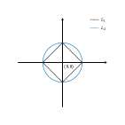
(a) Elastic-net

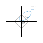
(b) Inertial Regularization and Selection (IRS)

Figure 1: Graphical illustration of proposed Inertial Regularization and Selection (IRS), and contrasting it with Elastic-net.

3.3 Why $\Sigma_{t|t-1}$ and $\theta_{t}^{*}$ adapted regularization?

In a sequential regularization model, it is critical to update the regularization penalties in a data driven manner. Otherwise, a repetitive regularization optimization for each epoch can be computationally cumbersome. We, therefore, use estimates of $\Sigma_{t|t-1}$ and $\theta_{t}^{*}$, which are derived from the data and have the necessary properties, discussed below, that results into an accurate model estimation.

For the inertia part, we want close to the expected value of $\theta_{t}$ given $\hat{\theta}_{t-1}$, i.e. $\hat{\theta}_{t|t-1}$. But the extent of regularization should be different for different $\theta_{t_{i}}$’s. The $\theta_{t_{i}}$ with higher expected variance should be regularized lesser. This is because, higher variance indicates that the $\theta_{t_{i}}$’s estimate from the past is not reliable. Thus, it should be learnt more from a recent data from epoch $t$ than keeping close to the past. And it is vice-versa if the expected variance of $\theta_{t_{i}}$ is small — tend to keep it close to a reliable past knowledge. Therefore, the inertia should be weighted by the inverse of the variance. Besides, as the correlations between the model parameters should be taken into account, as well, to adjust the changes in correlated parameters, we use $\Sigma_{t|t-1}^{-1}$ as an adaptive inertia weight.

In addition to the above intuition, $\Sigma_{t|t-1}^{-1}$ also stabilizes the inertial component. The inertial component can be regarded as a sum of residual squares from Eq. 1, i.e. we aim to minimize the residuals of $(\theta_{t}-\hat{\theta}_{t|t-1})$. Thus, the residual sum of squares should be scaled by its covariance, where $\Sigma_{t|t-1}=\text{cov}(\theta_{t}-\hat{\theta}_{t|t-1})$.

Besides, an adaptive penalty is applied on the $L_{1}$ norm for model selection. As suggested in [18], inverse of a reasonable estimate for $\theta$ provides a good adaptive penalty term for $L_{1}$ norm. [18] suggested an OLS estimate for a Lasso problem as a good estimate for the adaptive penalty, as it brings estimation consistency and guarantees oracle properties. As shown later, in §3.4, the IRS objective function in Eq. 4 is equivalent to a Lasso problem. From this Lasso equivalence, it can be seen that the OLS estimate desired for adaptively penalizing $\theta_{t}$ is same as an only inertia regularized estimate for $\theta_{t}$ , denoted as $\hat{\theta}_{t}^{*}$. The expression for $\hat{\theta}_{t}^{*}$ is derived and given in Appendix-B. We, therefore, use $\lambda/|\hat{\theta}_{t_{i}}^{*}|$ as penalty for the $\theta_{t_{i}}$’s $L_{1}$ regularization.

3.4 Lasso equivalence

Here we show a Lasso equivalent formulation of IRS. This is an important property because it shows IRS can inherit from a well developed pool of Lasso based techniques. In fact, the use of $\theta_{t}^{*}$ as the adaptive $L_{1}$ penalty for model selection is drawn from this Lasso equivalence. Besides, the estimation algorithm for IRS developed in §3.8 is also inspired from Lasso solutions.

The following shows the Lasso equivalence using a transformation and augmentation of data $X_{t}$ and $y_{t}$.

$$\begin{split}\tilde{X}_{t}=\left[\begin{array}[]{c}\frac{1}{\sqrt{2n_{t}}}W_{t}^{-\frac{1}{2}}X_{t}\\ \sqrt{\frac{\tau}{2p_{t}}}\Sigma_{t|t-1}^{-\frac{1}{2}}\end{array}\right];\>\>&\tilde{y}_{t}=\left[\begin{array}[]{c}\frac{1}{\sqrt{2n_{t}}}W_{t}^{-\frac{1}{2}}y_{t}\\ \sqrt{\frac{\tau}{2p_{t}}}\Sigma_{t|t-1}^{-1/2}\hat{\theta}_{t|t-1}\end{array}\right]\end{split}$$ (5)

Using transformed data in Eq. 5, we can rewrite the objective function in Eq. 4 as a Lasso problem, as given below (see Appendix-C for proof).

$$\mathcal{L}_{\hat{\theta}_{t-1}}(\theta_{t})=\left(\tilde{y}_{t}-\tilde{X}_{t}\theta_{t}\right){}^{T}\left(\tilde{y}_{t}-\tilde{X}_{t}\theta_{t}\right)+\frac{\lambda}{p_{t}}\sum_{i=1}^{p_{t}}\frac{|\theta_{t_{i}}|}{|\hat{\theta}_{t_{i}}^{*}|}$$ (6)

3.5 Kalman Filter as a special case

The Kalman Filter is found to be a special case of IRS. This finding highlights the commonality between filtering methods and regularization.

When $\lambda=0$, IRS becomes equivalent to a more general Kalman filter which has a weight adjusted state update, i.e. a weighted average of the state estimate from past and a Kalman estimate from the current data. The following shows the IRS estimate expression as equal to a Kalman filter expression (see Appendix-D for the proof).

$$\hat{\theta}_{t}^{*} = \left[X_{t}^{T}W_{t}^{-1}X_{t}+\tau^{*}\Sigma_{t|t-1}^{-1}\right]^{-1}\cdot$$ (7)

$$\left[X_{t}^{T}W_{t}^{-1}y_{t}+\tau^{*}\Sigma_{t|t-1}^{-1}\hat{\theta}_{t|t-1}\right]$$

$$= \hat{\theta}_{t|t-1}+\frac{1}{\tau^{*}}K_{t}(y_{t}-X_{t}\hat{\theta}_{t|t-1})$$

where, $K_{t}=\Sigma_{t|t-1}X_{t}^{T}\left(W_{t}+\frac{1}{\tau^{*}}X_{t}\Sigma_{t|t-1}X_{t}^{T}\right)^{-1}$ , also known as Kalman gain, and $\tau^{*}=\tau n_{t}/p_{t}$. As we can see above (Eq. 7), the expression for $\theta_{t}$ estimate is same as a conventional (unweighted) Kalman filter when $\tau^{*}=1$, and otherwise a weighted Kalman filter when $\tau^{*}$ is any other positive value. Besides, when $\tau^{*}=1$, the covariance of $\hat{\theta}_{t}^{*}$ can be shown to be same as in Kalman filter.

$$\Sigma_{t}^{*} = \text{cov}\left\{\left[X_{t}^{T}W_{t}^{-1}X_{t}+\Sigma_{t|t-1}^{-1}\right]^{-1}\cdot\right.$$ (8)

$$\left.\left[X_{t}^{T}W_{t}^{-1}y_{t}+\Sigma_{t|t-1}^{-1}\hat{\theta}_{t|t-1}\right]\right\}$$

$$= (I-K_{t}X_{t})\Sigma_{t|t-1}$$

It can be noted that, for estimating $\theta_{t}$ and $\Sigma_{t}$, the Kalman filter expression requires inverse of $K_{t}$. $K_{t}$, however, is a $n_{t}\times n_{t}$ matrix, inverting which can be computationally expensive when data size, $n_{t}$, is large. We provide an implementation for Kalman filter in Appendix-D, which is significantly faster for a usual scenario of $p_{t}<n_{t}$.

3.6 Equivalent Bayesian Formulation

The Bayesian formulation of IRS will have the following prior for $\theta$,

$$p_{\lambda,\tau}(\theta_{t})\propto\exp-\left(\frac{\lambda}{p_{t}}\sum_{i=1}^{p_{t}}\frac{|\theta_{t_{i}}|}{|\hat{\theta}_{t_{i}}^{*}|}\right)\cdot\\ \exp\left(-\frac{\tau}{2p_{t}}(\theta_{t}-\hat{\theta}_{t|t-1})^{T}\Sigma_{t|t-1}(\theta_{t}-\hat{\theta}_{t|t-1})\right)$$ (9)

This prior is a joint distribution of a double-exponential distribution for the $L_{1}$ penalty and a Gaussian centered around $\hat{\theta}_{t|t-1}$ and scaled with the covariance $\Sigma_{t|t-1}$ for the inertial $L_{2}$ penalty. The parameters $\theta_{t}$ can be estimated as the Bayes posterior mode (see Appendix-A).

3.7 Model covariance

Due to an $L_{1}$ norm term in the loss function, it is difficult to obtain an accurate estimate for the model covariance, $\Sigma_{t}$. Bootstraping can be a numerical way to estimate it. However, bootstrapping can be time consuming. Therefore, we propose an approximate closed form estimate, similar to the one proposed in [16]. In [16], the $L_{1}$ penalty $\sum|\theta_{i}|$ was replaced with $\sum\theta_{i}^{2}/|\theta_{i}|$, and the covariance matrix was approximated at the lasso estimate, $\hat{\theta}$, as a ridge regression expression.

This estimation, however, gives a 0 variance estimate if $\hat{\theta}_{i}$’s equal to 0. This is not desired in IRS, because a variance estimate for each $\theta_{i}$ is necessary for the inertial component. We, therefore, provide a slightly modified covariance expression, where $|\theta_{t_{i}}|$ is replaced by $\theta_{t_{i}}^{2}/|\hat{\theta}_{t_{i}}^{*}|$. Thus, an approximate covariance estimate is given as,

$$\Sigma_{t} = A_{t}^{-1}\left(X_{t}^{T}W_{t}^{-1}X_{t}+\tau^{*2}\Sigma_{t|t-1}^{-1}\right)A_{t}^{-1}$$ (10)

where,

$$A_{t} = X_{t}^{T}W_{t}^{-1}X_{t}+\lambda D_{t}^{-1}+\tau^{*}\Sigma_{t|t-1}^{-1}$$ (11)

$$D_{t} = \text{diag}\left(I(\hat{\theta}_{t_{i}}\neq 0)|\hat{\theta}_{t_{i}}||\hat{\theta}_{t_{i}}^{*}|+\right.$$ (12)

$$\left.(1-I(\hat{\theta}_{t_{i}}\neq 0))|\hat{\theta}_{t_{i}}^{*}|^{2};\,i=1,\ldots,p_{t}\right)$$

and $\tau^{*}=\tau n_{t}/p_{t}$.

3.8 Model Estimation

In this section, we first develop a closed form solution under orthogonality conditions, and then present an iterative proximal gradient estimation method for any general case. An algorithm is then laid out for implementing IRS in §3.8.3, where the various computational and implementation aspects are discussed.

3.8.1 Closed-form solution under orthogonality

The developed estimation technique possesses a closed-form solution if, (a) the predictors are orthonormal ($X_{t}^{T}X_{t}=I$), i.e. all columns in $X_{t}$ are linearly independent of each other, (b) the error of response model is i.i.d., $W_{t}=w_{t}^{2}I$, and, (c) the error covariance of the state model is i.i.d., $Q_{t}=q_{t}^{2}I$, which is often implied from if (a) is true.

Orthogonality conditions, a) $X_{t}^{T}X_{t}=I$, b) $W_{t}=w_{t}^{2}I$, and c) $Q_{t}=q_{t}^{2}I$. Under these conditions, $\Sigma_{t}$, and in turn $\Sigma_{t|t-1}$, will be diagonal matrices. Suppose we denote, $\Sigma_{t|t-1}=\boldsymbol{\rho}_{t}I$, where $\rho_{t_{i}}$ is the expected variance of $\theta_{t_{i}}$.

Plugging these conditions into Eq. 22, we get the OLS estimate expression as,

$$\hat{\theta}_{t}^{*} = \left(\frac{1}{w_{t}^{2}}I+\tau^{*}(\boldsymbol{\rho}_{t}I)^{-1}\right)^{-1}\left(\frac{1}{w_{t}^{2}}X_{t}^{T}y_{t}+\tau^{*}(\boldsymbol{\rho}_{t}I)^{-1}\hat{\theta}_{t|t-1}\right)$$ (13)

$$= (\boldsymbol{\rho}_{t}^{*}I)\left(\frac{1}{w_{t}^{2}}X_{t}^{T}y_{t}+\tau^{*}(\boldsymbol{\rho}_{t}I)^{-1}\hat{\theta}_{t|t-1}\right)$$

where, $\tau^{*}=\frac{\tau n_{t}}{p_{t}}$ and $\frac{1}{\rho_{t_{i}}^{*}}=\frac{1}{w_{t}^{2}}+\frac{\tau^{*}}{\rho_{t_{i}}},i=1,\ldots,p_{t}$.

We will use this expression to derive the IRS closed-form solution under orthogonality. From the Lasso equivalent formulation of IRS, the parameter estimate can be computed by minimizing, Eq. 6, i.e.,

$$\mathcal{L}(\theta_{t})=\left(\tilde{y}_{t}-\tilde{X}_{t}\theta_{t}\right){}^{T}\left(\tilde{y}_{t}-\tilde{X}_{t}\theta_{t}\right)+\frac{\lambda}{p_{t}}\sum_{i=1}^{p_{t}}\frac{|\theta_{t_{i}}|}{|\hat{\theta}_{t_{i}}^{*}|}$$ (14)

$$\arg\min_{\theta_{t}} -2\tilde{y}_{t}^{T}\tilde{X}_{t}\theta_{t}+\theta_{t}^{T}\tilde{X}_{t}^{T}\tilde{X}_{t}\theta_{t}+\frac{\lambda}{p_{t}}\sum_{i=1}^{p_{t}}\frac{|\theta_{t_{i}}|}{|\hat{\theta}_{t_{i}}^{*}|}$$

$$= -2\left(\frac{1}{2n_{t}}y_{t}^{T}W_{t}^{-1}X_{t}\theta_{t}+\frac{\tau}{2p_{t}}\hat{\theta}_{t|t-1}^{T}\Sigma_{t|t-1}^{-1}\theta_{t}\right)+$$

$$\frac{1}{2n_{t}}\theta_{t}^{T}X_{t}^{T}W_{t}^{-1}X_{t}\theta_{t}+\frac{\tau}{2p_{t}}\theta_{t}^{T}\Sigma_{t|t-1}^{-1}\theta_{t}+\frac{\lambda}{p_{t}}\sum_{i=1}^{p_{t}}\frac{|\theta_{t_{i}}|}{|\hat{\theta}_{t_{i}}^{*}|}$$

$$\propto -\left(\frac{1}{w_{t}^{2}}y_{t}^{T}X_{t}\theta_{t}+\tau^{*}(\boldsymbol{\rho}_{t}I)^{-1}\hat{\theta}_{t|t-1}^{T}\theta_{t}\right)+$$

$$\frac{1}{2w_{t}^{2}}\theta_{t}^{T}\theta_{t}+\tau^{*}(\boldsymbol{\rho}_{t}I)^{-1}\theta_{t}^{T}\theta_{t}+\frac{\lambda n_{t}}{p_{t}}\sum_{i=1}^{p_{t}}\frac{|\theta_{t_{i}}|}{|\hat{\theta}_{t_{i}}^{*}|}$$

$$= -\left(\frac{1}{w_{t}^{2}}y_{t}^{T}X_{t}+\tau^{*}(\boldsymbol{\rho}_{t}I)^{-1}\hat{\theta}_{t|t-1}^{T}\right)\theta_{t}+$$

$$\frac{1}{2}\left(\frac{1}{w_{t}^{2}}+\tau^{*}(\boldsymbol{\rho}_{t}I)^{-1}\right)\theta_{t}^{T}\theta_{t}+\frac{\lambda n_{t}}{p_{t}}\sum_{i=1}^{p_{t}}\frac{|\theta_{t_{i}}|}{|\hat{\theta}_{t_{i}}^{*}|}$$

$$= -(\boldsymbol{\rho}_{t}^{*}I)^{-1}\hat{\theta}_{t}^{*T}\theta_{t}+\frac{1}{2}(\boldsymbol{\rho}_{t}^{*}I)^{-1}\theta_{t}^{T}\theta_{t}+\frac{\lambda n_{t}}{p_{t}}\sum_{i=1}^{p_{t}}\frac{|\theta_{t_{i}}|}{|\hat{\theta}_{t_{i}}^{*}|}$$

$$= \sum_{i=1}^{p_{t}}-\frac{1}{\rho_{t_{i}}^{*}}\hat{\theta}_{t_{i}}^{*}\theta_{t_{i}}+\frac{1}{2\rho_{t_{i}}^{*}}\theta_{t_{i}}^{2}+\frac{\lambda n_{t}}{p_{t}}\frac{|\theta_{t_{i}}|}{|\hat{\theta}_{t_{i}}^{*}|}$$ (15)

\

On solving this for both cases when, $\theta_{i}^{(t)}\geq 0$ and $\leq 0$, we get the following solution,

$$\hat{\theta}_{t_{i}} = \text{sgn}(\hat{\theta}_{t_{i}}^{*})\left(\left|\hat{\theta}_{t_{i}}^{*}\right|-\frac{\lambda n_{t}}{p_{t}}\frac{\rho_{t_{i}}^{*}}{|\hat{\theta}_{t_{i}}^{*}|}\right)^{+}$$ (16)

where, $(\cdot)^{+}$ is a soft-thresholding function.

The components in the solution expression (Eq. 16) can be interpreted as a shrinkage on the inertia regularized parameter (OLS) estimate, $\hat{\theta}_{t_{i}}^{*}$, such that the amount of shrinkage is determined by, a) the magnitude of $\hat{\theta}_{t_{i}}^{*}$, for an adaptive variable selection from $L_{1}$ penalty, and b) $\rho_{t_{i}}^{*}$, which is proportional to the expected variance of the OLS estimate, $\hat{\theta}_{t_{i}}^{*}$, thus, IRS strongly shrinks $\hat{\theta}_{t_{i}}^{*}$ if its expected variance is high.

Therefore, parameters with high variance and low magnitude will be removed. The addition of variance element boosts the model selection capability to select a better model, resulting into a lower prediction errors.

3.8.2 Iterative estimation

Since, most commonly found problems do not satisfy an orthogonality condition, we develop a proximal gradient method to estimate the parameters in a general case.

$$\mathcal{L}(\theta_{t}) = \left\{\frac{1}{2n_{t}}\left(y_{t}-X_{t}\theta_{t}\right){}^{T}W_{t}^{-1}\left(y_{t}-X_{t}\theta_{t}\right)\right.+$$

$$\underbrace{\left.\frac{\tau}{2p_{t}}(\theta_{t}-\hat{\theta}_{t|t-1})^{T}\Sigma_{t|t-1}^{-1}(\theta_{t}-\hat{\theta}_{t|t-1})\right\}}_{f(\theta_{t})\rightarrow\text{differentiable}}$$

$$+\frac{\lambda}{p_{t}}\sum_{i=1}^{p_{t}}\frac{|\theta_{t_{i}}|}{|\hat{\theta}_{t_{i}}^{*}|}_{g(\theta_{t})\rightarrow\text{non-differentiable}}$$

$$= f(\theta_{t})+g(\theta_{t})$$

Since, $g$ is a $L_{1}$ function, an iterative proximal gradient algorithm will perform the following update,

$$\theta_{t_{i}}^{l+1} \leftarrow \text{Prox}_{\nu}\left(\theta_{t_{i}}^{l}-s^{l}\nabla f(\theta_{t_{i}}^{l})\right)$$ (17)

where, $\nu=\frac{\lambda s^{l}}{p_{t}|\hat{\theta}_{t_{i}}^{*}|}$ and $\text{Prox}_{\nu}(x)=\begin{cases}x-\nu&;x\geq\nu\\ 0&;|x|<\nu\\ x+\nu&;x\leq-\nu\end{cases}$ , $s^{l}$ is a step size for iteration $l$ (the step size can be kept same for all $l$ or decreased with increasing $l$) and

$$\nabla f(\theta_{t}^{l})=-\frac{1}{n_{t}}(X_{t})^{T}W_{t}^{-1}(y_{t}-X_{t}\theta_{t}^{l})+\frac{\tau}{p_{t}}\Sigma_{t|t-1}^{-1}(\theta_{t}^{l}-\hat{\theta}_{t|t-1})$$ (18)

Note that, any other estimation technique, for example, subgradient method or Least-Angle Regression (LARS), for estimating $\theta$. We chose proximal gradient method because of its ease of understanding and implementation. Besides, it performs well in most circumstances.

3.8.3 Algorithm

In this section, we present Algorithm-1 for implementing the iterative estimation method discussed above. The algorithm takes in the predictor matrices, $X_{t}$, and the responses, $y_{t}$, as they are collected for epoch $t=1,2,\ldots$. The $X_{t}$’s are standardized within each epoch $t$, such that the columns in $X_{t}$ has a mean of 0 and variance of 1. $y_{t}$, on the other hand, is centered to remove an intercept from the model.

The algorithm assumes $F_{t}$ and $Q_{t}$ as known inputs. In practice, $F_{t}$ is often set as equal to an identity matrix, $F_{t}=I$, and $Q_{t}$ as $\acute{o}^{2}I$, where $\acute{o}$ is a small positive number. Besides, the response error, $\epsilon_{t}$, in Eq. 2, is assumed as i.i.d., i.e. $W_{t}=w^{2}I$, and $p_{t}=p,\forall t$. While these are reasonable assumptions for most applications, it can be easily extended for circumstances outside of these assumptions.

As shown in Algorithm-1, the IRS estimation process starts from line-24. To initialize, an OLS estimate is computed, and residual sum of squares is used for obtaining $w^{2}$. Besides, the covariance is initialized as identity. Thereafter, for any $t$, $\hat{\theta}_{t|t-1}$, $\Sigma_{t|t-1}$ and $w^{2}$ (for approximating $W_{t}$) are computed and passed into ProximalDescent function, alongwith the data and regularization parameters, $(\lambda,\tau)$. This function implements the proximal gradient steps shown above in §3.8.2. Note that, it takes inverse of $\Sigma_{t|t-1}$ to save computation. Besides, it is recommended to have relatively larger data size in the initial epoch to avoid yielding a sub-optimal initial model.

A common issue in regularization models is tuning the penalty parameters, viz. $(\lambda,\tau)$ in IRS. It would have been even more challenging if IRS required to (re)tune $(\lambda,\tau)$ for each estimation epoch. However, due to the adaptive regularization developed in §3.3, it can be shown that the expected value of the loss function, $\mathcal{L}_{\hat{\theta}_{t-1}}(\theta_{t})$, remains a constant, i.e. independent of epoch t (see Appendix ??). This implies that an appropriately chosen $(\lambda,\tau)$ can be used for any $t=1,2,\ldots$.

Therefore, for IRS, we can use a k-fold cross validation (CV) on a two-dimensional grid search for $(\lambda,\tau)$, and model first few epochs for each grid point and measure their prediction errors. We used a 10-fold CV on first three epochs for $(\lambda,\tau)$ selection. Zou and Hastie (2005) have described this approach in detail and provided other possible selection approaches.

Computational time is another common issue in estimation procedures. The developed proximal gradient based algorithm has a fast convergence, which can be further boosted by changing the stepsize, $s$, for each iteration in line 11-18. This is common practice, with one simple approach as starting with a large value for $s$ and gradually decreasing it after each iteration. Another approach is to adaptively increase or decrease $s$ based on an increase or decrease in the residual error from $\theta_{t}^{l}$. Using this, the proximal gradient was found to converge in less than 50 iterations for upto 1000-dimensional models.

Besides, in implementation, operations in lines 13-16 can be vectorized and approximate matrix inversion methods can be used for a faster computation. Furthermore, accelerated proximal gradient and stochastic proximal gradient methods can be used to boost the computation.

1:$X_{t},y_{t},\hat{\theta}_{t-1},\Sigma_{t-1},\lambda,\tau,Q_{t};t=1,2,\ldots$  

2:function Prox($x,\nu$)

3:     $x\leftarrow\begin{cases}x-\nu&x>\nu\\ 0&|x|\leq\nu\\ x+\nu&x<-\nu\end{cases}$

4:     return $x$

5:end function

6:

7:function ProximalDescent($X_{t},y_{t},\hat{\theta}_{t|t-1},\newline \Sigma_{t|t-1}^{-1},w^{2},\lambda,\tau$)

8:     $n_{t}\leftarrow\arg_{n_{t}}X_{t}\in\mathbb{R}^{n_{t}\times p}$

9:     $\tau^{*}\leftarrow\tau n_{t}/p$

10:     $W_{t}\leftarrow w^{2}I_{n_{t}}$

11:     $\hat{\theta}_{t}^{*}\leftarrow(X_{t}^{T}W_{t}^{-1}X_{t}+\tau^{*}\Sigma^{-1}_{t|t-1})^{-1}(X_{t}^{T}W_{t}^{-1}{y}_{t}+\tau^{*}\Sigma^{-1}_{t|t-1}\hat{\theta}_{t|t-1})$

12:

13:     Initialize:

14:      $l=0,\theta_{t}^{0}=\hat{\theta}_{t}^{*},s$

15:     while $l<L$ do

16:         $\nabla f(\theta_{t}^{l})\leftarrow\frac{-1}{n_{t}}X^{T}_{t}W_{t}^{-1}(Y_{t}-X_{t}\theta_{t}^{l})+\frac{\tau}{p}\Sigma_{t|t-1}^{-1}(\theta_{t}^{l}-\hat{\theta}_{t|t-1})$

17:         for $i\in 1,\ldots,p$ do

18:              $\nu\leftarrow\frac{\lambda s}{p|\hat{\theta}^{*}_{t_{i}}|}$

19:              $\theta_{t_{i}}^{l}$ $\leftarrow$ Prox($\theta_{t_{i}}^{l}-s\nabla f(\theta_{t}^{l})_{i},\nu$)

20:         end for

21:         $l\leftarrow l+1$

22:     end while

23:     $D_{t}\leftarrow\text{Diag}(\mathbf{1}(\hat{\theta}_{t_{i}}\neq 0)|\hat{\theta}_{t_{i}}||\hat{\theta}_{t_{i}}^{*}|+(1-\mathbf{1}(\hat{\theta}_{t_{i}}\neq 0))|\hat{\theta}_{t_{i}}^{*}|^{2};i=1,\ldots,p)$

24:     $A_{t}\leftarrow X_{t}^{T}W_{t}^{-1}X_{t}+\lambda D_{t}^{-1}+\tau^{*}\Sigma^{-1}_{t|t-1}$

25:     $\Sigma_{t}\leftarrow A_{t}^{-1}(X_{t}^{T}W_{t}^{-1}X_{t}+{\tau^{*}}^{2}\Sigma_{t|t-1}^{-1})A_{t}^{-1}$

26:     return $\hat{\theta}_{t},\Sigma_{t}$

27:end function

28:

29:Initialize:

30:     

$n_{1}\leftarrow\arg_{n_{1}}X_{1}\in\mathbb{R}^{n_{1}\times p}$

$\hat{\theta}_{0}\leftarrow(X_{1}^{T}X_{1})^{-1}X_{1}y_{1}$

31:$w^{2}\leftarrow(y_{1}-X_{1}\hat{\theta}_{0})^{T}(y_{1}-X_{1}\hat{\theta}_{0})/(n_{1}-1)$

32:$\Sigma_{0}\leftarrow I_{p}$

33:IRS Estimation for, $t=1,2,\ldots$

34:$n_{t}\leftarrow\arg_{n_{t}}X_{t}\in\mathbb{R}^{n_{t}\times p}$

35:$\hat{\theta}_{t|t-1}\leftarrow F_{t}\hat{\theta}_{t-1}$

36:$\Sigma_{t|t-1}\leftarrow F_{t}\Sigma_{t-1}F_{t}^{T}+Q_{t}$

37:$w^{2}\leftarrow(y_{t}-X_{t}\hat{\theta}_{t|t-1})^{T}(y_{t}-X_{t}\hat{\theta}_{t|t-1})/(n_{t}-1)$

38:$\hat{\theta}_{t},\Sigma_{t}$ $\leftarrow$

39:ProximalDescent($X_{t},y_{t},\hat{\theta}_{t|t-1},\Sigma_{t|t-1}^{-1},w^{2},\lambda,\tau$)

40: 

41:Model estimate: $\hat{\theta}_{t},\Sigma_{t}$

Algorithm 1 Inertial Regularization and Selection (IRS) estimation

3.9 Ability to handle missing values and structural changes

A beneficial feature of IRS is the ease of handling missing values and any change in model structure. A change in model structure implies any addition or removal of model predictors. In case of missing values, IRS can still provide a reasonable parameter estimate in a modeling epoch by using the prior knowledge.

If a new predictor variable is added, for eg., one new product at Walmart, it can be easily incorporated in the modeling by expanding $\hat{\theta}_{t|t-1}$ and $\hat{\Sigma}_{t|t-1}$. If there is no expert prior knowledge for the new predictor, $\hat{\theta}_{t|t-1}$ can be expanded with 0 values and $\hat{\Sigma}_{t|t-1}$ with 0 off-diagonal (no correlation) and a large variance. This is same as an uninformative prior used is a Bayesian estimation. However, in several cases there is some expert knowledge. For instance, in the above Walmart example if the new product is a new baby diaper, we will have some knowledge for its parameter from similar products, and/or its correlations with other baby and related products.

Besides, IRS can handle removal of a predictor more cleverly than most other conventional methods. A removed predictor does not mean its effect will be gone immediately. In fact it will take some time before its effect vanishes completely. For eg. suppose a TV brand, say XYZ, is removed from a Walmart store, but since XYZ’s sales must be interacting with other TV sales, the effect of its absence will be felt for some time (maybe raising the demand for others) before gradually dying out. In IRS, it is not necessary to manually remove any predictor variable from the model even if we know it is physically removed. The inertial and selection component in IRS will automatically update the resultant effect and eventually remove the predictor variables from the model when its effect declines completely.

It is worthwhile to note that this IRS property also handles situations when the removal of the predictor is temporary. In the above Walmart eg., a reintroduction of the TV XYZ can be easily incorporated in the modeling updates, with the effect of reintroduction being the opposite of removal — the effect gradually increasing in the model.

This ability to easily handle missing values and structural changes in model is a valuable property because it makes the sequential modeling more robust to the real world scenarios.

4 Experimental Validation

In this section, we experimentally validate the efficacy of IRS. We compare it with Lasso, Kalman Filter (KF) and Ensemble KF (EnKF). Lasso was applied locally on each epoch $t$to show a prediction error baseline if the prior knowledge is ignored in sequential process. KF and EnKF are commonly used state-of-the-art state-space models against which IRS’s performance will be gauged.

We setup two types of experiments for validation, denoted as Exp-1 and Exp-2. In Exp-1, the number of model parameters (predictors) are kept same for all epochs, $p_{t}=p=\{500,5000\},t=1,2,\ldots,T$. The model parameters are randomly initialized for $t=1$ from a multivariate normal distribution with mean as 0, and an arbitrary covariance, such that a sparsity level of 0.2 is maintained. As the model enters from epoch $t$ to $t+1$, its parameters change with a random walk of variance 1. The sample size is randomly selected between $(1.8p,2.1p)$. The data is generated for 9 epochs, i.e. $T=9$. A 10-fold CV is performed on initial three epochs sample for regularization parameter selection. Thereafter, again a 10-fold CV is performed to fit each method, and the average test prediction error, rMSEs, are shown in Fig. 2a-2b.

The figures show that Lasso has a similar rMSE as IRS in the initial epoch. Thereafter, while Lasso’s prediction error remain approximately at the same level, IRS’s error reduces. This is due to the use of knowledge used from the past for updating the model with current data. KF and EnKF similar had a reducing error rates, however, they had a higher error than IRS and Lasso for the most of epochs. This can be attributed to their inability to work in a high-dimensional sparse processes. Besides, their performance seems to worsen when $p=5000$, compared to when $p=500$. This maybe due to KF and EnKF overfitting the data, resulting into higher test prediction errors, that gets higher as dimension increases.

In Exp-2, we initialized the model similar as Exp-1. However, for subsequent epochs, $t>1$, a parameter in $\theta_{t}$ was changed as, a) if $\theta_{t-1_{i}}$ is 0, it can become non-zero at $t$ with a small activation probability $(=0.05)$, and its value is again drawn from the initial multivariate normal distribution, b) if $\theta_{t-1_{i}}\neq 0$, then it can be deactivated (made equal to $0$) if it is less than a deactivation threshold $(=0.1)$ with a probability $(=0.1)$, c) if $\theta_{t-1_{i}}\neq 0$ and it is not deactivated, then it is changed with a random walk, $F_{t_{i}}=1$, or directionally $F_{t_{i}}=(1+N(0,0.1))$ with added random noise $(\sim N(0,1))$.

This setup emulates a real world problem where, an otherwise insignificant variable becomes significant and vice-versa, due to any systemic changes. Also, the shift in $\theta$ is sometimes directional, indicating an evolution. Regardless, we will perform the sequential modeling assuming $F_{t}=I$, to stay in tandem with the common state-space modeling practice.

In addition to incorporating evolution, we also reduce the data sample size for progressing epochs to test each methods’ efficacy in working with growing prior knowledge and lesser data.

Again, a 10-fold CV is performed and the average rMSEs from test prediction is reported in Fig. 3a-3b. As expected, the errors increase with passing epochs due to lesser sample size. While in the initial epochs, all methods have roughly the same error rate, it increases sharply for a localized Lasso fit. Between, EnKF and KF, the latters error rate grows faster and surpasses the rMSE of EnKF after some epochs pass. This can be due to EnKF’s better ability to estimate the parameter covariance even with lesser data (using the Monte Carlo setup). Among all, the increase in error rate is the lowest for IRS.

This result shows that IRS is also robust to the evolutionary model changes, and can work with lesser data as it garners more prior knowledge. This is an important feature for sequential modeling — indicating the ability of quickly updating the model as the system gets older.

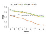
(a) $p=500$

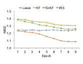
(b) $p=5000$

Figure 2: Exp-1: Average rMSE of test errors from a 10-fold cross validation.

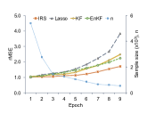
(a) $p=500$

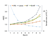
(b) $p=5000$

Figure 3: Exp-2: Average rMSE of test errors from a 10-fold cross validation.

The results in this section show the importance of use of past information for sequentially modeling data that arrives in a streaming fashion. For high-dimensional sparse and evolving models, it is shown that IRS outperforms the state-space models popular for such sequential modeling. Next, we will show a real world application of IRS.

5 Application on an online Retail Data

Here we show a real world application of IRS using a retail data from a UK-based and registered non-store online retail. The company mainly sells unique all-occasion gifts to mostly wholesalers and some individuals. The company was established in 1981 and relied on direct mailing catalogues. It went online in about 2010, since when it started accumulating huge amount of data.

A subset of that data used in this study lies between Dec, 2010 to Dec, 2011. The data is a customer transaction dataset, which has several variables, namely, product name, quantity sold, invoice date-time, unit price, customer-id, and country. For our analysis, we drop the variable customer-id, and select data from the country, UK. From this filtered data, we take a subset belonging to 41 products, such that it comprises of high to low selling items.

The “quantity sold” for a product in a transaction is the response variable, and the model’s objective is to predict it using all available predictors. For predictors, we extract the day-of-week and quarter-of-day from the invoice date-time to form predictors. Month is not taken because the data is for just one year, thus, deriving month seasonal effects will not be possible. Besides, other predictors are the unit price and product name. We create dummy columns for the categorical product name and day-of-week variables. Finally, a predictor matrix is made by taking in all predictor variables and their second-order interactions. Interaction effects are important to consider because sales of one product usually effects sales of some others. In total, the predictor matrix has 363 columns, that is, we have a 363-dimensional model.

Each month is treated as a modeling epoch. A 10-fold CV is performed on the first three epochs for penalty parameters, $(\lambda,\tau)$, selection, and then IRS is performed sequentially on all epochs. The 10-fold CV test prediction error (mean absolute percentage error, MAPE) in Fig. 5 show that IRS is more accurate than others. This is because several predictors in the above model will be statistically insignificant, thus, would require an effective model selection, in addition to use of the prior knowledge. However, as also mentioned before, KF and EnKF cannot effectively find a parsimonious model, and, thus, has poorer test accuracy.

In addition, we show another result of prediction errors for low selling products in Fig. 5. Demand forecast of low selling items are usually more difficult because of fewer available data. As shown in the figure, IRS again outperfoms other models. This can be attributed to IRS’s better capability is working with lesser data.

An online retail data, such as the one used here, is often very high-dimensional due to several categorical variables and interactions. Besides, the demand patterns typically have an inherent evolutionary characteristics. Note that, this evolution is different from the seasonalities and trend. Evolution is a gradual change due to various external factors, that are hard to measure. IRS is, thus, well suited for such problems. It can account for the evolutionary changes, and can handle high-dimensions, as well as, an automatic model selection.

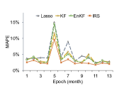
Figure 4: Forecasting accuracy for a randomly selected set of items.

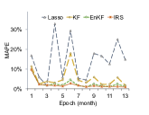
Figure 5: Forecasting accuracy for low selling items.

6 Discussion and Conclusion

In the previous section (§5), we show IRS’s superior prediction accuracy in an online retail data problem. This is an example of a high-dimensional statistical learning problem with sparsity and large data collection in a streaming fashion, where the process can also evolve. A majority of statistical learning problems found these days have similar properties. For instance, sensors data, telecommunications, weblogs, console logs, user music/movie play history (on services like spotify and Netflix), etc. Besides, in such problems various variables get added or removed from the process over time. Under all this fast-paced dynamics, IRS can be easily applied and yield a high accuracy.

In general, IRS’s ability to auto-tune its regularization parameters (given in §3.3) from the data makes it easy to implement. Due to this auto-tune ability, as further elucidated in §3.8.3, IRS has just two hyperparameters, $(\lambda,\tau)$, which if suitably selected provides an optimal solution for any epoch $t=1,2,\ldots$. However, in event of any abnormal or extreme system change, $(\lambda,\tau)$ may need to be re-tuned. Nevertheless, under normal conditions IRS provides a seamless sequential estimation for a statistical learning model.

Besides, the combination of inertial and $L_{1}$ penalty terms bring important properties of resemblance and model selection. Due to the inertia penalty, the model does not drastically change between epochs, thus, keeps a resemblance with what an analyst already knows about the model. The $L_{1}$ penalty provides an appropriate model selection on top of it. It must be noted that in model selection, the prior knowledge is also incorporated by using an adaptive penalty. This prevents the $L_{1}$ penalty from selecting an extremely different model than the past.

However, a potential downside of the resemblance property could be if the initial model is severely sub-optimal, the subsequent models can also be poor. In such cases, it may take several epochs for the model estimate to get close to the optimal. Therefore, to avoid this, it is recommended in §3.8.3 to use a larger amount of data in the initial epoch.

Regardless, IRS is also robust to noise and missing values due to the inertia component. This, alongwith an optimal model selection via $L_{1}$ penalty significantly boosts the test prediction accuracy, demonstrated in §4-5.

In this paper, we show IRS’s equivalence with Lasso, Kalman Filter and Bayesian estimation in §3.4-3.6. This also shows the interconnection between them for a statistical learning. Specifically, Kalman filters are often seen as a different family of estimators isolated from regularization techniques. Here, we establish their connection, and also present a faster implementation for Kalman filter in Appendix-D.

In summary, we develop a new method – Inertial Regularization and Selection (IRS) – for sequentially modelin an evolving statistical learning model. We present the modeling approach for a linear state-change (evolution) and a linear state-response model with gaussian errors. However, it can be easily extended to any non-linear model, if there is a link function transforming it into a linear form. For eg., a binary response in a classification model can be modeled using a logit-link for the state response model. The method is shown to outperform existing methods and several real world applications.

Appendix A Online recursive estimation loss function

The parameter estimate is a Bayesian formulation can be found from the Maximum a Posteriori (MAP) function, as shown below,

$$\{\hat{\theta}_{t}\}_{t=\{1,\ldots T\}} = \arg\max\left[\left(\prod_{t=1}^{T}p(\theta_{t}|\theta_{t-1})p(y_{t}|\theta_{t}\right)\right.$$ (19)

$$\left.p(y_{0}|\theta_{0})p(\theta_{0})\right]$$

$$= \arg\max\left[p(y_{T}|\theta_{T})p(\theta_{T}|\theta_{T-1})\right.\cdot$$

$$\left(\prod_{t=1}^{T-1}p(\theta_{t}|\theta_{t-1})p(y_{t}|\theta_{t})\right)$$

$$\left.p(y_{0}|\theta_{0})p(\theta_{0})\right]$$

A marginalization can be performed on Eq. 19 to find a globally optimal solution at the $T^{th}$ epoch.

$$\hat{\theta}_{T} = \arg\max_{\theta_{T}}\left[\int_{\mathbb{R}^{T}}p(y_{T}|\theta_{T})p(\theta_{T}|\theta_{T-1})\left(\prod_{t=1}^{T-1}p(\theta_{t}|\theta_{t-1})\cdot\right.\right.$$ (20)

$$\left.\left.p(y_{t}|\theta_{t})\right)\cdot p(y_{0}|\theta_{0})p(\theta_{0})d\{\theta_{i}\}_{i=1,\ldots,T-1}\right]$$

$$= \arg\max\left[p(y_{T}|\theta_{T})p(\theta_{T}|\theta_{T-1})\int_{\mathbb{R}^{T}}\left(\prod_{t=1}^{T-1}p(\theta_{t}|\theta_{t-1})\cdot\right.\right.$$

$$\left.\left.p(y_{t}|\theta_{t})\right)p(y_{0}|\theta_{0})p(\theta_{0})d\{\theta_{i}\}_{i=1,\ldots,T-1}\right]$$

The integral part in Eq. 20 is essentially the prior on $\theta_{T}$. Thus, for an online estimation, the updated form of Eq. 19 for $\theta_{T}$, given below, can be used.

$$\hat{\theta}_{T} = \arg\max_{\theta_{T}}p(y_{T}|\theta_{T})p_{\hat{\theta}_{T-1}}(\theta_{T})$$ (21)

Eq. 21 summarizes all the past information from the likelihood $\theta_{T}|\{y_{t}\}_{t=1,\ldots,T-1}$ into the prior for $\theta_{T}$ given $\hat{\theta}_{T-1}$. Using the Bayesian prior distribution for IRS given in §3.6, into Eq. 21, we get,

$$\hat{\theta}_{T} = \arg\max_{\theta_{T}}\exp\left[-(y_{T}-X_{T}\theta_{T})^{T}W_{T}^{-1}(y_{T}-X_{T}\theta_{T})\right]\cdot$$

$$\exp\left[-\tau(\theta_{T}-\hat{\theta}_{T|T-1})^{T}\Sigma_{T|T-1}^{-1}(\theta_{T}-\hat{\theta}_{T|T-1})-\right.$$

$$\left.\sum\lambda_{t_{i}}\frac{|\theta_{T_{i}}|}{|\hat{\theta}_{T_{i}}^{*}|}\right]$$

$$= \arg\min_{\theta_{T}}(y_{T}-X_{T}\theta_{T})^{T}W_{T}^{-1}(y_{T}-X_{T}\theta_{T})+$$

$$\tau(\theta_{T}-\hat{\theta}_{T|T-1})^{T}\Sigma_{T|T-1}^{-1}(\theta_{T}-\hat{\theta}_{T|T-1})+\sum\lambda_{t_{i}}\frac{|\theta_{T_{i}}|}{|\hat{\theta}_{T_{i}}^{*}|}$$

Appendix B OLS estimate for the LASSO equivalent

The OLS estimate, denoted by $\hat{\theta}_{t}^{*}$ , for IRS can be easily found from its lasso equivalent given in Eq. 6, in §3.4.

$$\hat{\theta}_{t}^{*} = (\tilde{X}_{t}^{T}\tilde{X}_{t})^{-1}\tilde{X}_{t}^{T}\tilde{y}_{t}$$ (22)

$$= \left(\frac{1}{2n_{t}}X_{t}^{T}W_{t}^{-1}X_{t}+\frac{\tau}{2p_{t}}\Sigma_{t|t-1}^{-1}\right)^{-1}\cdot$$

$$\left(\frac{1}{2n_{t}}X_{t}^{T}W_{t}^{-1}y_{t}+\frac{\tau}{2p_{t}}\Sigma_{t|t-1}^{-1}\hat{\theta}_{t|t-1}\right)$$

$$= \left(X_{t}^{T}W_{t}^{-1}X_{t}+\tau^{*}\Sigma_{t|t-1}^{-1}\right)^{-1}\left(X_{t}^{T}W_{t}^{-1}y_{t}+\tau^{*}\Sigma_{t|t-1}^{-1}\hat{\theta}_{t|t-1}\right)$$

where, $\tau^{*}=\frac{\tau n_{t}}{p_{t}}$.

Appendix C Proving LASSO equivalence

Using an augmented $X$ and $y$ in Eq. 5, we need to show,

$$(\tilde{y}_{t}-\tilde{X}_{t}\theta_{t})^{T}(\tilde{y}_{t}-\tilde{X}_{t}\theta_{t})_{\text{L.H.S.}}$$

$$= \left[\frac{1}{2n_{t}}(Y_{t}-X_{t}\theta_{t})^{T}W_{t}^{-1}(Y_{t}-X_{t}\theta_{t})+\right.$$

$$\left.\frac{\tau}{2p_{t}}(\theta_{t}-\hat{\theta}_{t|t-1})^{T}\Sigma_{t|t-1}^{-1}(\theta_{t}-\hat{\theta}_{t|t-1})\right]_{\text{R.H.S.}}$$

To prove L.H.S. is equal to R.H.S., we expand L.H.S.:

$$(\tilde{y}_{t}-\tilde{X}_{t}\theta_{t})^{T}(\tilde{y}_{t}-\tilde{X}_{t}\theta_{t})$$

$$= \tilde{y}_{t}^{T}\tilde{y}_{t}-2\tilde{y}_{t}^{T}\tilde{X}_{t}\theta_{t}+\theta_{t}^{T}\tilde{X}_{t}^{T}\tilde{X}_{t}\theta_{t}$$

$$= \frac{1}{2n_{t}}y_{t}^{T}W_{t}^{-1}y_{t}+\frac{\tau}{2p_{t}}\hat{\theta}_{t|t-1}^{T}\Sigma_{t|t-1}^{-1}\hat{\theta}_{t|t-1}$$

$$-2\left(\frac{1}{2n_{t}}y_{t}^{T}W_{t}^{-1}X_{t}\theta_{t}+\frac{\tau}{2p_{t}}\hat{\theta}_{t|t-1}^{T}\Sigma_{t|t-1}^{-1}\theta_{t}\right)$$

$$+\frac{1}{2n_{t}}\theta_{t}^{T}X_{t}^{T}W_{t}^{-1}X_{t}\theta_{t}+\frac{\tau}{2p_{t}}\theta_{t}^{T}\Sigma_{t|t-1}^{-1}\theta_{t}$$

$$= \frac{1}{2n_{t}}\left(y_{t}^{T}W_{t}^{-1}y_{t}-2y_{t}^{T}W_{t}^{-1}X_{t}\theta_{t}+\theta_{t}^{T}X_{t}^{T}W_{t}^{-1}X_{t}\theta_{t}\right)$$

$$+\frac{\tau}{2p_{t}}\left(\theta_{t}^{T}\Sigma_{t|t-1}^{-1}\theta_{t}-2\hat{\theta}_{t|t-1}^{T}\Sigma_{t|t-1}^{-1}\theta_{t}+\hat{\theta}_{t|t-1}^{T}\Sigma_{t|t-1}^{-1}\hat{\theta}_{t|t-1}\right)$$

$$= \frac{1}{2n_{t}}(y_{t}-X_{t}\theta_{t})^{T}W_{t}^{-1}(y_{t}-X_{t}\theta_{t})+$$

$$\frac{\tau}{2p_{t}}(\theta_{t}-\hat{\theta}_{t|t-1})^{T}\Sigma_{t|t-1}^{-1}(\theta_{t}-\hat{\theta}_{t|t-1})$$

$$=$$ R.H.S.

Appendix D Showing Kalman Filter Equivalence

Here we expand the IRS expression for $\theta_{t}$ estimate when $\lambda=0$, denoted by $\hat{\theta}_{t}^{*}$, given in Eq. 22 in Appendix-B.

$$\hat{\theta}_{t}^{*} = \left[X_{t}^{T}W_{t}^{-1}X_{t}+\tau^{*}\Sigma_{t|t-1}^{-1}\right]^{-1}\cdot$$ (23)

$$\left[X_{t}^{T}W_{t}^{-1}y_{t}+\tau^{*}\Sigma_{t|t-1}^{-1}\hat{\theta}_{t|t-1}\right]$$

$$= \left[\frac{1}{\tau^{*}}\Sigma_{t|t-1}-\frac{1}{\tau^{*}}K_{t}X_{t}\frac{1}{\tau^{*}}\Sigma_{t|t-1}\right]\cdot$$

$$\left[X_{t}^{T}W_{t}^{-1}y_{t}+\tau^{*}\Sigma_{t|t-1}^{-1}\hat{\theta}_{t|t-1}\right]$$

$$= \hat{\theta}_{t|t-1}-\frac{1}{\tau^{*}}K_{t}X_{t}\hat{\theta}_{t|t-1}+$$

$$\left[\frac{1}{\tau^{*}}\Sigma_{t|t-1}X_{t}^{T}W_{t}^{-1}-\frac{1}{(\tau^{*})^{2}}K_{t}X_{t}\Sigma_{t|t-1}X_{t}^{T}W_{t}^{-1}\right]y_{t}$$

$$= \hat{\theta}_{t|t-1}-\frac{1}{\tau^{*}}K_{t}X_{t}\hat{\theta}_{t|t-1}+$$

$$K_{t}\left[\frac{1}{\tau^{*}}\left(W_{t}+\frac{1}{\tau^{*}}X_{t}\Sigma_{t|t-1}X_{t}^{T}\right)W_{t}^{-1}-\right.$$

$$\left.\frac{1}{(\tau^{*})^{2}}X_{t}\Sigma_{t|t-1}X_{t}^{T}W_{t}^{-1}\right]y_{t}$$

$$= \hat{\theta}_{t|t-1}+\frac{1}{\tau^{*}}K_{t}(y_{t}-X_{t}\hat{\theta}_{t|t-1})$$

where, $K_{t}=\Sigma_{t|t-1}X_{t}^{T}\left(W_{t}+\frac{1}{\tau^{*}}X_{t}\Sigma_{t|t-1}X_{t}^{T}\right)^{-1}$ , also known as Kalman gain.

Besides, when $\tau^{*}=1$, the covariance of $\hat{\theta}_{t}^{*}$ can be shown to be same as in Kalman filter.

$$\Sigma_{t}^{*} = \text{cov}\left\{\underbrace{\left[X_{t}^{T}W_{t}^{-1}X_{t}+\Sigma_{t|t-1}^{-1}\right]}_{E_{t}}^{-1}\cdot\right.$$

$$\left.\left[X_{t}^{T}W_{t}^{-1}y_{t}+\Sigma_{t|t-1}^{-1}\hat{\theta}_{t|t-1}\right]\right\}$$

$$= E_{t}^{-1}X_{t}^{T}W_{t}^{-1}\text{cov}(y_{t})W_{t}^{-1}X_{t}^{T}E_{t}^{-1}+$$

$$E_{t}^{-1}\Sigma_{t|t-1}^{-1}\text{$\hat{\theta}_{t|t-1}$}\Sigma_{t|t-1}^{-1}E_{t}^{-1}$$

$$= E_{t}^{-1}\left(X_{t}^{T}W_{t}^{-1}X_{t}^{T}+\Sigma_{t|t-1}^{-1}\right)E_{t}^{-1}$$

$$= E_{t}^{-1}E_{t}E_{t}^{-1}$$

$$= \left(X_{t}^{T}W_{t}^{-1}X_{t}^{T}+\Sigma_{t|t-1}^{-1}\right)^{-1}$$

$$= \Sigma_{t|t-1}-$$

$$\Sigma_{t|t-1}X_{t}^{T}\left(W_{t}+X_{t}\Sigma_{t|t-1}X_{t}^{T}\right)^{-1}X_{t}\Sigma_{t|t-1}$$

$$= \Sigma_{t|t-1}-K_{t}X_{t}\Sigma_{t|t-1}$$

$$= (I-K_{t}X_{t})\Sigma_{t|t-1}$$

Faster Kalman filter algorithm

Given a previous estimate of $\theta$ and its covariance, as $\hat{\theta}_{t-1}$ and $\Sigma_{t-1}$, and the data, the updated model is found using the following steps,

$$\hat{\theta}_{t|t-1} = F_{t}\hat{\theta}_{t-1}$$ (24)

$$\Sigma_{t|t-1} = F_{t}\Sigma_{t-1}F_{t}^{T}+Q_{t}$$ (25)

$$K_{t} = \Sigma_{t|t-1}X_{t}^{T}\left(\Sigma_{t}+X_{t}\Sigma_{t|t-1}X_{t}^{T}\right)^{-1}$$ (26)

$$\hat{\theta}_{t} = \hat{\theta}_{t|t-1}+K_{t}\left(y_{t}-X_{t}\hat{\theta}_{t|t-1}\right)$$ (27)

$$\Sigma_{t} = \left(I-K_{t}X_{t}\right)\Sigma_{t|t-1}$$ (28)

The formulation shows an evolving model as an additive function of the prior model. However, computationally it becomes intensive if the datasize is even reasonably large. This is due to a $n_{t}\times n_{t}$ matrix inversion required in Eq. 26. Using the IRS equivalence for Kalman, we can have the following procedure for Kalman filter estimation, which is significantly faster when $p<n_{t}$, i.e. the number of parameters being less than the datasize, which is more common in statistical learning models (unlike the signal processing model, a primary focus for Kalman filters).

A faster algorithm for Kalman will, thus, replace Eq. 26-28 as,

$$\hat{\theta}_{t} = \left[X_{t}^{T}R_{t}^{-1}X_{t}+\Sigma_{t|t-1}^{-1}\right]^{-1}\left[X_{t}^{T}R_{t}^{-1}y_{t}+\Sigma_{t|t-1}^{-1}\hat{\theta}_{t|t-1}\right]$$

$$\Sigma_{t} = \left(X_{t}^{T}R_{t}^{-1}X_{t}+\Sigma_{t|t-1}^{-1}\right)^{-1}$$

Appendix E Stationarity of IRS loss function

The IRS loss function given in Eq. 4 has three components. Here we will show that they are individually stationary, meaning they have a constant expectation, independent of time epochs.

$$\mathcal{L}_{\hat{\theta}_{t-1}}(\theta_{t}) = \underbrace{\frac{1}{2n_{t}}(y_{t}-X_{t}\theta_{t})^{T}W_{t}^{-1}(y_{t}-X_{t}\theta_{t})}_{(\text{A})}+$$ (29)

$$\underbrace{\frac{\tau}{2p_{t}}(\theta_{t}-\hat{\theta}_{t|t-1})^{T}\Sigma_{t|t-1}^{-1}(\theta_{t}-\hat{\theta}_{t|t-1})}_{(\text{B})}+$$

$$\underbrace{\frac{\lambda}{p_{t}}\sum_{i=1}^{p_{t}}\frac{|\theta_{t_{i}}|}{|\hat{\theta}_{t_{i}}^{*}|}}_{(\text{C})}$$

We will use the following identity applicable for a random variable, $x\sim N(\mu,\Sigma)$, and any known matrix $A$.

$$E[x^{T}Ax] = \text{Tr}(A\Sigma)+\mu^{T}A\mu$$ (30)

• Part $(\text{A})$: $y_{t}-X_{t}\theta_{t}\sim N(0,W_{t})$, where $W_{t}$ is a symmetric matrix. Therefore, $E[(\text{A})]=\frac{1}{2n_{t}}\left(\text{Tr}(W_{t}^{-1}W_{t})+0\right)=\frac{1}{2n_{t}}n_{t}=\frac{1}{2}$.

• Part $(\text{B})$: $\theta_{t}-\hat{\theta}_{t|t-1}\sim N(0,\Sigma_{t|t-1})$. Similarly, as for part $(\text{A})$, we will have, $E[(\text{B})]=\frac{\tau}{2}$.

• Part $(\text{C})$: Suppose, $\theta_{t_{i}}$ is approximated as a hard-thresholded estimate from OLS, $\theta_{t_{i}}=\hat{\theta}_{t_{i}}^{*}\cdot\epsilon_{t_{i}}^{*}$, where $\epsilon_{t_{i}}^{*}\sim\text{Bernoulli}(\alpha)$. Therefore, $E\left[\left|\frac{\theta_{t_{i}}}{\hat{\theta}_{t_{i}}^{*}}\right|\right]=\alpha\implies E[(\text{C})]=\lambda\alpha$. Here, $\alpha$ can be interpreted as the proportion of variables that are selected from the $L_{1}$ penalization. Assuming $\alpha$ is same for all epochs, the expectation of part $(\text{C})$ is independent of $t$.

References

- [1] E. Candes and J. Romberg. Sparsity and incoherence in compressive sampling. Inverse problems, 23(3):969, 2007.
- [2] E. J. Candes, M. B. Wakin, and S. P. Boyd. Enhancing sparsity by reweighted 1 minimization. Journal of Fourier analysis and applications, 14(5-6):877–905, 2008.
- [3] A. Carmi, P. Gurfil, and D. Kanevsky. Methods for sparse signal recovery using kalman filtering with embedded pseudo-measurement norms and quasi-norms. IEEE Transactions on Signal Processing, 58(4):2405–2409, 2010.
- [4] A. Charles, M. S. Asif, J. Romberg, and C. Rozell. Sparsity penalties in dynamical system estimation. In Information Sciences and Systems (CISS), 2011 45th Annual Conference on, pages 1–6. IEEE, 2011.
- [5] A. S. Charles and C. J. Rozell. Dynamic filtering of sparse signals using reweighted 1. In 2013 IEEE International Conference on Acoustics, Speech and Signal Processing, pages 6451–6455. IEEE, 2013.
- [6] Y. Ding and X. Li. Time weight collaborative filtering. In Proceedings of the 14th ACM international conference on Information and knowledge management, pages 485–492. ACM, 2005.
- [7] G. Evensen. The ensemble kalman filter: Theoretical formulation and practical implementation. Ocean dynamics, 53(4):343–367, 2003.
- [8] N. J. Gordon, D. J. Salmond, and A. F. Smith. Novel approach to nonlinear/non-gaussian bayesian state estimation. In IEE Proceedings F-Radar and Signal Processing, volume 140, pages 107–113. IET, 1993.
- [9] S. J. Julier and J. K. Uhlmann. Unscented filtering and nonlinear estimation. Proceedings of the IEEE, 92(3):401–422, 2004.
- [10] R. E. Kalman. A new approach to linear filtering and prediction problems. Journal of basic Engineering, 82(1):35–45, 1960.
- [11] J. Lei and P. Bickel. Ensemble filtering for high dimensional non-linear state space models. University of California, Berkeley, Rep, 779:23, 2009.
- [12] J. S. Liu. Monte Carlo strategies in scientific computing. Springer Science & Business Media, 2008.
- [13] E. Ott, B. R. Hunt, I. Szunyogh, A. V. Zimin, E. J. Kostelich, M. Corazza, E. Kalnay, D. Patil, and J. A. Yorke. A local ensemble kalman filter for atmospheric data assimilation. Tellus A, 56(5):415–428, 2004.
- [14] R. L. Plackett. Some theorems in least squares. Biometrika, 37(1/2):149–157, 1950.
- [15] D. Sejdinovic, C. Andrieu, and R. Piechocki. Bayesian sequential compressed sensing in sparse dynamical systems. In Allerton Conf. Communication, Control, and Computing. Citeseer, 2010.
- [16] R. Tibshirani. Regression shrinkage and selection via the lasso. Journal of the Royal Statistical Society. Series B (Methodological), pages 267–288, 1996.
- [17] N. Vaswani. Kalman filtered compressed sensing. In 2008 15th IEEE International Conference on Image Processing, pages 893–896. IEEE, 2008.
- [18] H. Zou. The adaptive lasso and its oracle properties. Journal of the American statistical association, 101(476):1418–1429, 2006.