Enhancement of small-scale turbulent dynamo by large-scale shear

Abstract

Small-scale dynamos are ubiquitous in a broad range of turbulent flows with large-scale shear, ranging from solar and galactic magnetism to accretion disks, cosmology and structure formation. Using high-resolution direct numerical simulations we show that in non-helically forced turbulence with zero mean magnetic field, large-scale shear supports small-scale dynamo action, i.e., the dynamo growth rate increases with shear and shear enhances or even produces turbulence, which, in turn, further increases the dynamo growth rate. When the production rates of turbulent kinetic energy due to shear and forcing are comparable, we find scalings for the growth rate $\gamma$ of the small-scale dynamo and the turbulent velocity $u_{\rm rms}$ with shear rate $S$ that are independent of the magnetic Prandtl number: $\gamma\propto|S|$ and $u_{\rm rms}\propto|S|^{2/3}$. For large fluid and magnetic Reynolds numbers, $\gamma$, normalized by its shear-free value, depends only on shear. Having compensated for shear-induced effects on turbulent velocity, we find that the normalized growth rate of the small-scale dynamo exhibits the scaling, $\widetilde{\gamma}\propto|S|^{2/3}$, arising solely from the induction equation for a given velocity field.

1. Introduction

In an electrically conducting turbulent fluid, the dynamo is a fundamental phenomenon that can explain the origin of magnetic fields in solar like stars, galaxies, accretion discs, etc. Two types of turbulent dynamos are usually discussed in the literature: large-scale and small-scale dynamos (see, e.g., Moffatt, 1978; Zeldovich et al., 1990; Brandenburg & Subramanian, 2005). Magnetic field generation on scales smaller and larger than the integral scale of turbulence are described as small-scale dynamo (SSD) and large-scale dynamo (LSD), respectively. The small-scale dynamos are ubiquitous and naturally find applications in a broad range of topics such as galactic magnetism (Kulsrud & Anderson, 1992; Rieder & Teyssier, 2016), solar coronal heating (Amari et al., 2015), accretion disks (Blackman & Nauman, 2015), cosmology and structure formation (Pakmor, 2014), Riemannian manifolds (Sokoloff & Rubashny, 2013), formation of the first stars in the Universe (Schleicher et al., 2010), etc.

The nature of the SSD depends strongly on the magnetic Prandtl number, ${\rm Pr}_{\rm M}=\nu/\eta$ (see, e.g., Kulsrud & Anderson, 1992; Schekochihin et al., 2004; Haugen et al., 2004; Schekochihin et al., 2005; Brandenburg, 2011), where $\eta$ is the magnetic diffusivity due to the electrical conductivity of the plasma and $\nu$ is its kinematic viscosity. Random stretching of the magnetic field by smooth velocity fluctuations in the viscous subrange of scales describes the small-scale dynamo for ${\rm Pr}_{\rm M}\gg 1$ (see, e.g., Zeldovich et al., 1990; Kleeorin & Rogachevskii, 1994; Subramanian, 1998; Kleeorin et al., 2002; Bhat & Subramanian, 2014; Schekochihin et al., 2004; Haugen et al., 2004; Schekochihin et al., 2005). The small-scale dynamo at low ${\rm Pr}_{\rm M}$ is excited by the turbulent inertial-range velocity fluctuations (the spatially rough velocity field). The growth rate of the small-scale dynamo at low ${\rm Pr}_{\rm M}$ is determined by the resistive magnetic diffusion scale (see, e.g., Kazantsev, 1968; Vainshtein & Zeldovich, 1972; Rogachevskii & Kleeorin, 1997; Boldyrev & Cattaneo, 2004; Iskakov et al., 2007; Schekochihin et al., 2007; Schober et al., 2012).

Large-scale velocity shear is a common feature of many astrophysical flows in, e.g., solar and stellar convective zones, galaxies, accretion disks (see, e.g., Moffatt, 1978; Zeldovich et al., 1990; Brandenburg & Subramanian, 2005). In recent years, a non-helical turbulent shear dynamo has been discussed, where the presence of large-scale shear in turbulence with zero mean kinetic helicity yields a large-scale dynamo (see, e.g., Vishniac & Brandenburg, 1997; Sokoloff, 1997; Rogachevskii & Kleeorin, 2003; Brandenburg, 2005; Kleeorin & Rogachevskii, 2008; Yousef et al., 2008; Brandenburg et al., 2008; Käpylä et al., 2008; Sridhar & Subramanian, 2009; Sridhar & Singh, 2010; Singh & Sridhar, 2011; Sridhar & Singh, 2014). The main conclusion from these studies is that a combination of homogeneous non-helical turbulence and large-scale shear is able to generate a large-scale magnetic field without any mean kinetic helicity. Like many other large-scale turbulent dynamos, they yield pronounced large-scale magnetic structures. Large-scale shear in non-helical turbulence also causes a “vorticity dynamo”, i.e., the excitation of a large-scale instability, resulting in an exponential growth of the mean vorticity (Elperin et al., 2003; Yousef et al., 2008; Käpylä et al., 2009).

In turbulence with large-scale shear, the SSD can be strongly affected by shear, notably because turbulence itself can be produced by the shear. However, the details related to the effect of shear on the small-scale dynamo are unclear. Recent analytical study by Kolokolov et al. (2011) has demonstrated that, for a given random smooth velocity field, large-scale shear can support a small-scale dynamo, such that the dynamo growth rate, which we denote as $\widetilde{\gamma}$ arising solely from the induction equation, increases with shear rate $S$ as $\widetilde{\gamma}\propto|S|^{2/3}$. This is compatible with an upper bound for growth rates discussed in Proctor (2012).

In this Letter, we study the effects of large-scale shear on a small-scale dynamo using high-resolution direct numerical simulations (DNS) for different magnetic Prandtl numbers ranging from 0.5 to 10. Using the budget equation for turbulent kinetic energy, we develop a framework for identifying a scaling function that we then determine in DNS. In agreement with earlier work by Kolokolov et al. (2011), we demonstrate that the growth rate of a SSD in non-helically forced turbulence increases with the shear rate.

2. Budget equation

Since large-scale shear can affect the turbulent velocity, we start with a theoretical analysis based on the budget equation for turbulent kinetic energy, ${\cal E}_{\rm K}={\textstyle{1\over 2}}\overline{{\bm{u}}^{2}}$, assuming incompressibility (Monin & Yaglom, 1971):

$${D{\cal E}_{\rm K}\over Dt}+{\rm div}\,{\bm{\Phi}}_{\rm K} = -\overline{u_{i}\,u_{j}}\,\nabla_{j}\overline{U}_{i}+\overline{{\bm{u}}{\bm{\cdot}}{\bm{f}}_{\rm f}}-\varepsilon,$$ (1)

where $D/Dt=\partial/\partial t+\overline{\bm{U}}{\bm{\cdot}}{\bm{\nabla}}$ is the advective derivative, ${\bm{u}}$ is the fluctuating velocity, $\overline{\bm{U}}$ is the mean velocity, and $\varepsilon$ is the dissipation rate of ${\cal E}_{\rm K}$. The term ${\bm{\Phi}}_{\rm K}=\rho^{-1}\overline{{\bm{u}}\,p}+\overline{{\bm{u}}\,u^{2}}/2$ includes the third-order moments that determine the flux of ${\cal E}_{\rm K}$, where $p$ are the pressure fluctuations, and $\rho$ is the fluid density. The term $\overline{{\bm{u}}{\bm{\cdot}}{\bm{f}}_{\rm f}}$ in Equation (1) describes the production rate of turbulence caused by external forcing, while the first term in the right hand side of Equation (1) determines the turbulence production rate caused by large-scale shear.

The Reynolds stresses in isotropic turbulence are (Monin & Yaglom, 1971; Elperin et al., 2002):

$$\overline{u_{i}\,u_{j}}={\overline{u^{2}}\over 3}\,\delta_{ij}-{\nu_{{}_{\rm T}}\over 2}\,\left(\nabla_{i}\overline{U}_{j}+\nabla_{j}\overline{U}_{i}\right),$$ (2)

where $\nu_{{}_{\rm T}}$ is the turbulent viscosity and $\delta_{ij}$ is the Kronecker tensor. Let us consider for simplicity turbulence with a linear velocity shear, $\overline{\bm{U}}=(0,Sx,0)$, which results in anisotropy of turbulence. However, the modification of the Reynolds stresses by anisotropic turbulence does not change the turbulence production rate caused by linear velocity shear; see Equations (A33) and (12) in Elperin et al. (2002). The dissipation rate of ${\cal E}_{\rm K}$ for large fluid Reynolds numbers is estimated as $\varepsilon\sim{\cal E}_{\rm K}/\tau_{\rm f}=u_{\rm rms}^{3}/2\ell_{\rm f}$ (Monin & Yaglom, 1971), while the turbulent viscosity is estimated as $\nu_{{}_{\rm T}}\sim\ell_{\rm f}\,u_{\rm rms}/3$, where $\ell_{\rm f}$ is the integral scale of the turbulence, $u_{\rm rms}=\sqrt{\overline{{\bm{u}}^{2}}}$ and $\tau_{\rm f}=\ell_{\rm f}/u_{\rm rms}$ is the characteristic turbulent time based on the integral scale.

Substituting Equation (2) into Equation (1) we obtain:

$${D{\cal E}_{\rm K}\over Dt}+{\rm div}\,{\bm{\Phi}}_{\rm K}=\overline{{\bm{u}}{\bm{\cdot}}{\bm{f}}_{\rm f}}+{\nu_{{}_{\rm T}}\over 2}\,S^{2}-{u_{\rm rms}^{3}\over 2\ell_{\rm f}}.$$ (3)

Depending on the value of shear, Equation (3) implies the following scalings for $u_{\rm rms}(S)$ in stationary homogeneous turbulence:

(i) Small shear: the turbulent production rate caused by the forcing is much larger than that caused by the shear, so that $u_{0}^{3}/2\ell_{\rm f}\sim\overline{{\bm{u}}{\bm{\cdot}}{\bm{f}}_{\rm f}}$, and $\nu_{{}_{\rm T}}=\nu_{{}_{\rm T}}^{(0)}\sim\ell_{\rm f}\,u_{0}/3$, where $u_{0}=u_{\rm rms}(S=0)$. For small shear, $u_{\rm rms}$ is weakly dependent on shear.

(ii) Intermediate shear: the turbulent production rates caused by the forcing and the shear are of the same order, and the balance, $u_{\rm rms}^{3}/\ell_{\rm f}\sim\nu_{{}_{\rm T}}^{(0)}S^{2}$, yields the following scaling: $u_{\rm rms}\propto|S|^{2/3}$.

(iii) Strong shear: the turbulent production rate in Equation (3) caused by the forcing can be neglected, so that turbulence is produced only by shear. The steady-state solution of the equation, $\nu_{{}_{\rm T}}S^{2}-u_{\rm rms}^{3}/\ell_{\rm f}=0$, yields the scaling $u_{\rm rms}=S\,\ell_{\rm f}$. This implies that for shear-produced turbulence, the small-scale shear rate $u_{\rm rms}/\ell_{\rm f}$ cannot be much smaller than the large-scale shear.

3. Growth rate of the small-scale dynamo

Let us consider first the case ${\rm Pr}_{\rm M}\ll 1$, when the resistive magnetic diffusion scale is much larger than the Kolmogorov viscous scale. This implies that the resistive scale is located inside the inertial range of the turbulence, where the fluid motions are spatially rough. The small-scale dynamo occurs due to random stretching of the magnetic field by the turbulent velocity, while scale-dependent turbulent magnetic diffusivity causes dissipation of the magnetic field. At the resistive scale, the scale-dependent turbulent magnetic diffusivity approaches $\eta$. The strongest magnetic field stretching is at small scales, i.e., at the resistive scale. Therefore, the growth rate of the small-scale dynamo (far from the threshold) in turbulence without large-scale shear for ${\rm Pr}_{\rm M}\ll 1$ is estimated as the inverse resistive time (see, e.g., Kazantsev, 1968; Schekochihin et al., 2007):

$$\gamma_{0}\sim u_{\eta}/\ell_{\eta}\sim\tau_{\rm f}^{-1}\,{\rm Re}_{\rm M}^{1/2},$$ (4)

where $u_{\eta}=(\varepsilon\,\ell_{\eta})^{1/3}$ is the characteristic turbulent velocity at the resistive scale, $\ell_{\eta}$, and ${\rm Re}_{\rm M}$ is the magnetic Reynolds number.

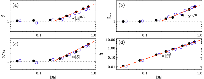
Figure 1.— Shear dependencies of (a) $\widetilde{\gamma}$, (b) $\widetilde{u}_{\rm rms}$, (c) $\gamma/\gamma_{0}$, and (d) $\widetilde{\Pi}$, shown for two choices of ${\rm Pr}_{\rm M}$, both sets having $u_{\max}/c_{\rm s}=0.07$, and $|S|_{\max}/c_{\rm s}k_{\rm f}=0.02$. Filled (black) circles: ${\rm Pr}_{\rm M}=0.5$ with $\gamma_{0}/u_{0}k_{\rm f}=0.02$, and ${\rm Re}_{\rm M}^{(0)}\equiv u_{0}/k_{\rm f}\eta=121$; open (blue) circles: ${\rm Pr}_{\rm M}=3$, with $\gamma_{0}/u_{0}k_{\rm f}=0.05$, and ${\rm Re}_{\rm M}^{(0)}\equiv u_{0}/k_{\rm f}\eta=148$.

Using Equation (4), we assume that the growth rate of the small-scale dynamo instability with large-scale shear, normalized by that without shear, can be estimated as

$$\frac{\gamma(S)}{\gamma_{0}}\sim\left(\frac{u_{\rm rms}(S)}{u_{0}}\right)^{1/2}\,\widetilde{\gamma}(S),$$ (5)

where $\gamma_{0}=\gamma(S=0)$ and $u_{0}=u_{\rm rms}(S=0)$ represent the dynamo growth rate and the rms velocity for $S=0$, and $\widetilde{\gamma}(S=0)=1$. Let us define the normalized rms velocity, $\widetilde{u}_{\rm rms}=u_{\rm rms}(S)/u_{0}$. Here we assumed that the turbulent forcing scale, $\ell_{\rm f}$, is independent of large-scale shear. The contribution $\widetilde{u}_{\rm rms}^{1/2}$, to the dynamo growth rate is caused by the effect of large-scale shear on the turbulent velocity field, while the function $\widetilde{\gamma}(S)$ determines the effect of large-scale shear on the growth of the small-scale dynamo instability for a given turbulent velocity field. Thus the normalized growth rate, $\widetilde{\gamma}$, which can be interpreted as a contribution to the dynamo growth rate arising solely from the induction equation for a given velocity field, can be expressed as

$$\widetilde{\gamma}=\gamma(S)\Big{/}\left(\gamma_{0}\,\,\sqrt{\widetilde{u}_{\rm rms}}\right)\,.$$ (6)

It is useful to define the ratio of the turbulent production rates caused by shear and forcing,

$$\widetilde{\Pi}=\frac{\Pi_{S}}{\Pi_{\rm f}}=\frac{\nu_{{}_{\rm T}}S^{2}}{u_{\rm rms}f}=\frac{2\pi S^{2}}{3k_{\rm f}f}\,.$$ (7)

For ${\rm Pr}_{\rm M}\gg 1$, magnetic fluctuations are determined by the smooth velocity field in the viscous subrange. We assume that in turbulence with large-scale shear, Equation (5) is also valid for ${\rm Pr}_{\rm M}\geq 1$. In the next section we perform DNS to determine the scaling laws for $\gamma(S)/\gamma_{0}$ and $u_{\rm rms}(S)/u_{0}$.

4. Numerical setup

We consider low-Mach-number compressible isothermal magnetohydrodynamic turbulence with background shear, $\overline{\bm{U}}^{S}=(0,Sx,0)$ with $S<0$, and a white-noise nonhelical random statistically homogeneous isotropic body force $f$ as the source of turbulent motions. The departure $U$ from the mean shear flow obeys

$${{\cal D}{}\mbox{\boldmath$U$}{}\over{\cal D}{}t}=-\mbox{\boldmath$U$}{}\cdot\mbox{\boldmath$\nabla$}{}\mbox{\boldmath$U$}{}+SU_{x}\hat{\mbox{\boldmath$y$}}{}-c_{\rm s}^{2}\mbox{\boldmath$\nabla$}{}\ln\rho+\rho^{-1}\mbox{\boldmath$J$}{}\times\mbox{\boldmath$B$}{}$$

$$\quad\quad\quad+\mbox{\boldmath$f$}{}+\mbox{\boldmath$F$}{}_{\rm visc},$$ (8)

$${{\cal D}{}\ln\rho\over{\cal D}{}t}=-\mbox{\boldmath$U$}{}\cdot\mbox{\boldmath$\nabla$}{}\ln\rho-\mbox{\boldmath$\nabla$}{}\cdot\mbox{\boldmath$U$}{},$$ (9)

$${{\cal D}{}\mbox{\boldmath$A$}{}\over{\cal D}{}t}=-SA_{y}\hat{\mbox{\boldmath$x$}}{}+\mbox{\boldmath$U$}{}\times\mbox{\boldmath$B$}{}-\eta\mbox{\boldmath$J$}{}\,,$$ (10)

where ${\cal D}{}/{\cal D}{}t\equiv\partial_{t}+Sx\,\nabla_{y}$ is the advective derivative with respect to $\overline{\bm{U}}^{S}$, $\mbox{\boldmath$B$}{}=\mbox{\boldmath$\nabla$}{}\times\mbox{\boldmath$A$}{}$ is the magnetic field in terms of the vector potential $A$, $\mbox{\boldmath$F$}{}_{\rm visc}=\rho^{-1}\mbox{\boldmath$\nabla$}{}\cdot(2\nu\rho\mbox{\boldmath${\sf S}$}{})$ is the viscous force, ${\sf S}_{ij}={\textstyle{1\over 2}}(\nabla_{i}U_{j}+\nabla_{j}U_{i})-{\textstyle{1\over 3}}\delta_{ij}\mbox{\boldmath$\nabla$}{}\cdot\mbox{\boldmath$U$}{}$ is the traceless rate of strain tensor, $\mbox{\boldmath$J$}{}=\mbox{\boldmath$\nabla$}{}\times\mbox{\boldmath$B$}{}/\mu_{0}$ is the current density, $\mu_{0}$ is the vacuum permeability, and $c_{\rm s}$ is the isothermal sound speed. These equations are solved with shearing-periodic boundary conditions using the Pencil Code (https://github.com/pencil-code). It uses sixth-order explicit finite differences in space and a third-order accurate time-stepping method.

We solve Equations (8)–(10) in a cubic domain of size $L^{3}$ using $512^{3}$ or $1024^{3}$ spatial resolution and choose $k_{\rm f}=2.2\,k_{1}$, where $k_{1}=2\pi/L$. Thus the chosen stochastic forcing injects energy at scales close to the box-scale. This allows us to study the SSD in the absence of the large-scale dynamo (LSD), or the so-called shear dynamo, that is also expected to be excited in such a setup. However, the LSD would require a reasonably larger scale separation. Nevertheless, the growth rates measured from an early kinematic stage predominantly reflect the growth of SSD which grows at a rate much faster than that of the possible LSD.

The system of equations is characterized by the following set of non-dimensional numbers:

$${\rm Re}_{\rm M}=\frac{u_{\rm rms}}{\eta k_{\rm f}},\quad\mbox{\rm Re}=\frac{u_{\rm rms}}{\nu k_{\rm f}},\quad{\rm Pr}_{\rm M}=\frac{\nu}{\eta},$$

$$\mbox{{\rm Sh}}=\frac{S}{u_{0}\,k_{\rm f}},\quad\widetilde{\rm S}{\rm h}=\frac{S}{u_{\rm rms}\,k_{\rm f}},\quad\Sigma_{\rm f}=\frac{c_{\rm s}\,\nu k_{1}^{2}}{f}$$ (11)

where Re and ${\rm Re}_{\rm M}$ are the fluid and magnetic Reynolds numbers, ${\rm Pr}_{\rm M}$ is the magnetic Prandtl number, Sh and $\widetilde{\rm S}{\rm h}$ are the shear parameters based on $u_{0}$ and $u_{\rm rms}$, respectively, and $\Sigma_{\rm f}$ characterizes the inverse forcing.

5. DNS results

In this section we discuss the results of DNS and compare with the theoretical predictions.

5.1. The dynamo growth rate and production of turbulence

First we determine the small-scale dynamo growth rate as a function of $S$. To this end we drop the Lorentz force in the momentum equation (8). In Fig. 1 we show the shear dependencies of (i) the normalized dynamo growth rate, $\widetilde{\gamma}(S)$ which is defined by Equation (6), (ii) the normalized rms velocity, $\widetilde{u}_{\rm rms}=u_{\rm rms}(S)/u_{0}$, (iii) total growth rate $\gamma$, and (iv) the ratio of turbulence production rates $\widetilde{\Pi}$, for two values of ${\rm Pr}_{\rm M}$ (smaller and larger than unity). Figure 1 demonstrates the existence of the following scalings for intermediate shear when the ratio $\widetilde{\Pi}$ is of the order of unity:

$$\gamma/\gamma_{0}\propto|S|,\quad\widetilde{u}_{\rm rms}\propto|S|^{2/3},\quad\widetilde{\gamma}\propto|S|^{2/3}\,.$$ (12)

These scalings are independent of ${\rm Pr}_{\rm M}$. The small-scale dynamo growth rate increases with shear, which implies that large-scale shear supports the small-scale dynamo. The obtained DNS scaling for $\widetilde{\gamma}$ coincides with that found by Kolokolov et al. (2011) from solution of the equation for the pair correlation function of the magnetic field. This equation was derived from the induction equation for a given random smooth velocity field.

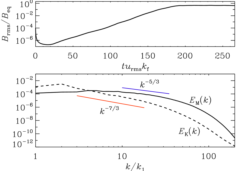
Figure 2.— Nonlinear evolution of $B_{\rm rms}/B_{\rm eq}$ (upper panel) and spectra of magnetic $E_{\rm M}(k)$ (solid) and kinetic $E_{\rm K}(k)$ (dashed) energies in the saturation stage (lower panel) at ${\rm Pr}_{\rm M}=10$ with $|\widetilde{\rm S}{\rm h}|=0.23$, $u_{\rm rms}/c_{\rm s}=0.04$ and $|S|/c_{\rm s}k_{\rm f}=0.009$.

5.2. Nonlinear stage of the SSD

In Fig. 2 we plot the nonlinear evolution of $B_{\rm rms}/B_{\rm eq}$ and spectra of magnetic, $E_{\rm M}(k)$, and kinetic, $E_{\rm K}(k)$, energies in the saturation stage, where $B_{\rm eq}=(\mu_{0}\rho)^{1/2}u_{\rm rms}$ is the equipartition magnetic field. Magnetic fluctuations reach saturation at the equipartition level and have a short inertial range compatible with a $k^{-5/3}$ spectrum. At larger scales, the velocity is compatible with a $k^{-7/3}$ spectrum which is expected for anisotropic sheared fluctuations produced by tangling of the large-scale gradient of the mean velocity by the background random velocity field. This spectrum was predicted analytically by Lumley (1967), detected in atmospheric turbulence by Wyngaard & Cote (1972) and confirmed in DNS by Ishihara et al. (2002).

Figure 3 shows results based on $1024^{3}$ simulations at ${\rm Pr}_{\rm M}=10$ for varying forcing strengths while keeping the shear-rate $S$ as fixed. The turbulence is produced by shear in all three cases, which yields the same $u_{\rm rms}$ in the saturated state, thus resulting in the same value for the shear parameter $\widetilde{\rm S}{\rm h}$. The growth rates of SSD are found to be identical, as would be expected from our above findings. Note that the onset of the dynamo growth is delayed for weaker forcing (e.g., red curve in Fig. 3).

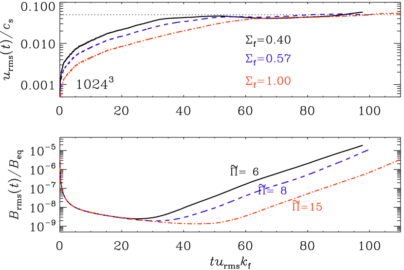
Figure 3.— Temporal evolution of $u_{\rm rms}$ and $B_{\rm rms}$ from three runs with solid, dashed, and dash-dotted curves in the order of decreased forcing, while all other parameters are the same: ${\rm Pr}_{\rm M}=10$, $\mbox{\rm Re}=220$, $|\widetilde{\rm S}{\rm h}|=0.3$, $u_{\rm rms}/c_{\rm s}=0.05$, and $|S|/c_{\rm s}k_{\rm f}=0.02$. For all three cases we find $\gamma/u_{\rm rms}k_{\rm f}=0.146$.

5.3. Mean-flow generation

Figure 2 demonstrates the fact that shear fundamentally modifies the nature of background turbulence, resulting in a $k^{-7/3}$ spectrum, which leads to the generation of a large-scale flow. In Fig. 4 we show a space-time diagram of the mean flow components, $\overline{U}_{x}$ and $\overline{U}_{y}$, where the mean is obtained by applying a planar (here $xy$) average. Both $\overline{U}_{x}$ and $\overline{U}_{y}$ spontaneously develop a mean pattern in the direction normal to the shear plane. Such a generation of mean flow has been first explored by Elperin et al. (2003) and numerically demonstrated by Yousef et al. (2008); Käpylä et al. (2009). The mean flow pattern begins to develop after a few tens of eddy turnover time, $(u_{\rm rms}k_{\rm f})^{-1}$. We found that $\overline{U}_{y}$ is about four times stronger compared to $\overline{U}_{x}$ and both are excited in phase, which is in agreement with Käpylä et al. (2009).

5.4. Saturation of the shear parameter

Based on $512^{3}$ simulations at magnetic Prandtl number ${\rm Pr}_{\rm M}=0.5$ and $3$, we showed in Fig. 1b that the $u_{\rm rms}$ increases with shear. The dimensionless shear parameter, $\widetilde{\rm S}{\rm h}$, defined with respect to $u_{\rm rms}(S)$, is thus expected to approach saturation at large shear rates in the regime of shear-produced turbulence. Here we check the saturation of $\widetilde{\rm S}{\rm h}$ by performing a suite of lower resolution, $128^{3}$, simulations at ${\rm Pr}_{\rm M}=1$. For a fixed shear rate, we explore the shear-produced turbulence regime (i.e., the regime with $\widetilde{\Pi}>1$) by successively decreasing the forcing strength, i.e., by increasing $\Sigma_{\rm f}$; see Equations (7) and (11) for definitions of $\widetilde{\Pi}$ and $\Sigma_{\rm f}$, respectively.

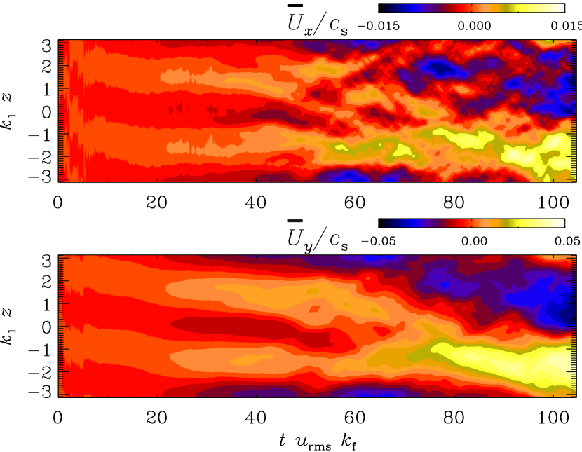
Figure 4.— $\overline{U}_{x}$ (top) and $\overline{U}_{y}$ (bottom) as functions of time and $z$ from a $1024^{3}$ simulation with ${\rm Pr}_{\rm M}=10$, $|\widetilde{\rm S}{\rm h}|=0.3$, $\widetilde{\Pi}=15$ and $u_{\rm rms}/c_{\rm s}=0.046$.

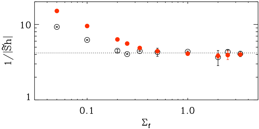
Figure 5.— Saturation of the shear parameter $\widetilde{\rm S}{\rm h}$ as a function of $\Sigma_{\rm f}$ for two choices of shear-rate, $|S|/c_{\rm s}k_{\rm f}=0.022$ (black, open circles) and $|S|/c_{\rm s}k_{\rm f}=0.013$ (red, filled circles), both at ${\rm Pr}_{\rm M}=1$. Larger values of $\Sigma_{\rm f}$ corresponds to the regime where the turbulence is predominantly produced by shear. The dotted line represents $|\widetilde{\rm S}{\rm h}|=3/4\pi$.

In Fig. 5, we demonstrate the saturation of the shear parameter, $\widetilde{\rm S}{\rm h}$ as a function of $\Sigma_{\rm f}$. Two different choices of the shear rate result in the overlap of $1/|\widetilde{\rm S}{\rm h}|$ at large values of $\Sigma_{\rm f}$ and show saturation at a constant level corresponding to $|\widetilde{\rm S}{\rm h}|\approx 3/4\pi$. Thus, in a realistic setup with subsonic turbulence, such as the one being studied here, it would not be possible to explore values of $|\widetilde{\rm S}{\rm h}|$ that are much larger than about $0.25$. Note that the abscissae in Fig. 1 correspond to Sh which is defined with respect to $u_{0}$, instead of $u_{\rm rms}(S)$, and therefore extend up to about unity.

The effect of shear on the SSD becomes noticeable only when shear-rate exceeds certain threshold such that the turbulence production ratio, $\widetilde{\Pi}$, becomes of order unity or larger. This results in a narrow range of possible values for the shear parameter to determine the scalings of the SSD growth rates versus shear rate. Thus, one interesting regime of a very strong shear is not found in DNS.

6. Discussion

It is worth noting that recent simulations by Tobias & Cattaneo (2013) of a prescribed deterministic non-helical flow with large-scale shear and a superposition of small-scale cellular deterministic flows, have shown that large-scale shear reduces the small-scale dynamo growth rate. In those simulations, the Navier-Stokes equation is not used, so the effects of shear-produced turbulence, whereby large-scale shear increases the turbulent velocity, have been ignored. As a result, shear suppresses the small-scale dynamo by a sweeping effect, i.e., the shear de-correlates the small eddies from the magnetic field by advecting the field. On the other hand, in our study a different setup is used, where large-scale shear fundamentally modifies and even produces turbulence, and enhances the efficiency of the small-scale dynamo. Notably, the generation of non-uniform mean velocity field, as shown in Fig. 4, was not observed in Tobias & Cattaneo (2013). This additionally confirms the difference between their setup and ours.

Remarkably, we obtain from DNS the same scaling, $\widetilde{\gamma}(S)\propto|S|^{2/3}$, for SSD growth rate as was theoretically predicted by Kolokolov et al. (2011) for a given velocity field. Interestingly, the occurrences of intermittent shear bursts were found to amplify the growth of the SSD in turbulent magnetoconvection (Pratt et al., 2013).

7. Conclusions

Using DNS, it was demonstrated that the small-scale dynamo growth rate increases with shear in nonhelical turbulence. The scalings for the growth rate of the small-scale dynamo, $\gamma\propto|S|$, and for the turbulent velocity, $u_{\rm rms}\propto|S|^{2/3}$, are independent of ${\rm Pr}_{\rm M}$, when the turbulent production rates caused by shear and forcing are of the same order. The contribution to the dynamo growth rate, $\widetilde{\gamma}\propto|S|^{2/3}$, is also found to be independent of ${\rm Pr}_{\rm M}$. This contribution is determined solely by the equation for the pair correlation function of the magnetic field derived from the induction equation.

We found that large-scale shear has the following three different effects that are relevant for turbulent small-scale dynamo:

1. Direct effect of shear on the generation of small-scale magnetic fields through the induction equation.

2. Production of turbulence by the shear which further enhances the SSD action.

3. Generation of large-scale non-uniform motions due to interaction of turbulence with mean shear by the vorticity dynamo, which in turn produces new large-scale shear, thus enhancing the SSD.

References

- Amari et al. (2015) Amari, T., Luciani, J., & Aly, J. 2015, Nature, 522, 188
- Bhat & Subramanian (2014) Bhat, P., & Subramanian, K. 2014, Astrophys. J., 791, L34
- Blackman & Nauman (2015) Blackman, E. G., & Nauman, F. 2015, J. Plasma Phys., 81, 395810505
- Boldyrev & Cattaneo (2004) Boldyrev, S., & Cattaneo, F. 2004, Phys. Rev. Lett., 92, 144501
- Brandenburg (2005) Brandenburg, A. 2005, Astrophys. J., 625, 539
- Brandenburg (2011) Brandenburg, A. 2011, Astrophys. J., 741, 92
- Brandenburg & Subramanian (2005) Brandenburg, A., & Subramanian, K. 2005, Phys. Rep., 417, 1
- Brandenburg et al. (2008) Brandenburg, A., Rädler,K.-H., Rheinhardt, M., & Käpylä, P. J. 2008, Astrophys. J., 676, 740
- Elperin et al. (2003) Elperin, T., Kleeorin, N., & Rogachevskii, I. 2003, Phys. Rev. E, 68, 016311
- Elperin et al. (2002) Elperin, T., Kleeorin, N., Rogachevskii, I., & Zilitinkevich, S. S., 2002, Phys. Rev. E, 66, 066305
- Ishihara et al. (2002) Ishihara, T., Yoshida, K., & Kaneda, Y. 2002, Phys. Rev. Lett., 88, 154501
- Iskakov et al. (2007) Iskakov, A. B., Schekochihin, A. A., Cowley, S. C., McWilliams, J. C., & Proctor, M. R. E. 2007, Phys. Rev. Lett., 98, 208510
- Haugen et al. (2004) Haugen, N. E. L., Brandenburg, A., & Dobler, W. 2004, Phys. Rev. E, 70, 016308
- Kulsrud & Anderson (1992) Kulsrud, R. M., & Anderson, S. W. 1992, Astrophys. J., 396, 606
- Kazantsev (1968) Kazantsev, A. P. 1968, Sov. Phys. JETP, 26, 1031
- Käpylä et al. (2008) Käpylä, P. J., Korpi, M. J., & Brandenburg, A. 2008, A&A, 491, 353
- Käpylä et al. (2009) Käpylä, P. J., Mitra, D., & Brandenburg, A. 2009, Phys. Rev. E, 79, 016302
- Kleeorin & Rogachevskii (1994) Kleeorin, N., & Rogachevskii, I. 1994, Phys. Rev. E, 50, 493
- Kleeorin & Rogachevskii (2008) Kleeorin, N., & Rogachevskii, I. 2008, Phys. Rev. E, 77, 036307
- Kleeorin & Rogachevskii (2012) Kleeorin, N., & Rogachevskii, I. 2012, Phys. Scr., 86, 018404
- Kleeorin et al. (2002) Kleeorin, N., Rogachevskii, I., & Sokoloff, D. 2002, Phys. Rev. E, 65, 036303
- Kolokolov et al. (2011) Kolokolov, I. V., Lebedev, V. V., & Sizov, G. A. 2011, J. Exper. Theor. Phys., 113, 339
- Lumley (1967) Lumley, J. L. 1967, Phys. Fluids, 10, 1405
- Moffatt (1978) Moffatt, H. K., Magnetic Field Generation in Electrically Conducting Fluids (Cambridge University Press, New York, 1978).
- Monin & Yaglom (1971) Monin, A. S., & Yaglom, A. M., Statistical Fluid Mechanics (MIT Press, Cambridge, Massachusetts, 1971), Vol. 1.
- Pakmor (2014) Pakmor, R., Marinacci, F., & Springel, V. 2014, ApJ, 783, L20
- Pratt et al. (2013) Pratt, J., Busse, A., & Müller, W.-C. 2013, A&A, 557, A76
- Proctor (2012) Proctor, M. R. E. 2012, J. Fluid Mech., 697, 504
- Rieder & Teyssier (2016) Rieder, M., & Teyssier, R. 2016, MNRAS, 457, 1722
- Rogachevskii & Kleeorin (1997) Rogachevskii, I., & Kleeorin, N. 1997, Phys. Rev. E, 56, 417
- Rogachevskii & Kleeorin (2003) Rogachevskii, I., & Kleeorin, N. 2003, Phys. Rev. E, 68, 036301
- Schekochihin et al. (2004) Schekochihin, A. A., Cowley, S. C., Taylor, S. F., Maron, J. L., & McWilliams, J. C. 2004, Astrophys. J., 612, 276
- Schekochihin et al. (2005) Schekochihin, A. A., Haugen, N. E. L., Brandenburg, A., Cowley, S. C., Maron, J. L., & McWilliams, J. C. 2005, Astrophys. J., 625, L115
- Schekochihin et al. (2007) Schekochihin, A. A., Iskakov, A. B., Cowley, S. C., McWilliams, J. C., Proctor, M. R. E., & Yousef, T. A. 2007, New J. Phys., 9, 300
- Schleicher et al. (2010) Schleicher, D. R. G., Banerjee, R., Sur, S., Arshakian, T. G., Klessen, R. S., Beck, R., & Spaans, M. 2010, A&A, 522, A115
- Schober et al. (2012) Schober, J., Schleicher, D., Federrath, Ch., Klessen, R., & Banerjee, R. 2012, Phys. Rev. E, 85, 026303
- Singh & Sridhar (2011) Singh, N. K., & Sridhar, S. 2011, Phys. Rev. E, 83, 056309
- Soker (2017) Soker, N. 2017, MNRAS, 466, 4776
- Sokoloff (1997) Sokoloff, D. D. 1997, Astron. Rep., 41, 68
- Sokoloff & Rubashny (2013) Sokoloff, D., & Rubashny, A. 2013, Geophys. Astrophys. Fluid Dyn., 107, 403
- Sridhar & Singh (2010) Sridhar, S., & Singh, N. K. 2010, J. Fluid Mech., 664, 265
- Sridhar & Singh (2014) Sridhar, S., & Singh, N. K. 2014, MNRAS, 445, 3770
- Sridhar & Subramanian (2009) Sridhar, S., & Subramanian, K. 2009, Phys. Rev. E, 80, 066315
- Subramanian (1998) Subramanian, K. 1998, MNRAS, 294, 718
- Tobias & Cattaneo (2013) Tobias, S. M., & Cattaneo, F. 2013, Nature, 497, 463
- Vainshtein & Zeldovich (1972) Vainshtein, S. I., & Zeldovich, Ya. B. 1972, Sov. Phys. Usp., 15, 159
- Vishniac & Brandenburg (1997) Vishniac, E. T., & Brandenburg, A. 1997, Astrophys. J., 475, 263
- Wyngaard & Cote (1972) Wyngaard, J. C., & Cote, O. R. 1972, Q. J. R. Meteorol. Soc., 98, 590
- Yousef et al. (2008) Yousef, T. A., Heinemann, T., Schekochihin, A. A., Kleeorin, N., Rogachevskii, I., Iskakov, A. B., Cowley, S. C., & McWilliams, J. C. 2008a, Phys. Rev. Lett., 100, 184501
- Zeldovich et al. (1990) Zeldovich, Ya. B., Ruzmaikin, A. A., & Sokoloff, D. D., The Almighty Chance (Word Scientific Publ., London, 1990).