Sets of Priors Reflecting Prior-Data Conflict and Agreement

Abstract

In Bayesian statistics, the choice of prior distribution is often debatable, especially if prior knowledge is limited or data are scarce. In imprecise probability, sets of priors are used to accurately model and reflect prior knowledge. This has the advantage that prior-data conflict sensitivity can be modelled: Ranges of posterior inferences should be larger when prior and data are in conflict. We propose a new method for generating prior sets which, in addition to prior-data conflict sensitivity, allows to reflect strong prior-data agreement by decreased posterior imprecision.

1 Introduction

The Bayesian approach to inference [6] offers the advantage to combine data and prior expert knowledge in a unified reasoning process. It combines a parametric sample model, denoted by a conditional distribution $f({\bm{x}}\mid\vartheta)$ of data ${\bm{x}}=(x_{1},\ldots,x_{n})$ given parameter $\vartheta$ with a prior distribution $f(\vartheta)$, expressing expert opinion on $\vartheta$. Given ${\bm{x}}$, the prior distribution is updated by Bayes’ Rule to obtain the posterior distribution $f(\vartheta\mid{\bm{x}})\propto f({\bm{x}}\mid\vartheta)\cdot f(\vartheta)$. The choice of prior distribution is often debatable. One can employ sensitivity analysis to study the effect of different prior distributions on the inferences, as done in robust Bayesian methods [2]. The method presented in this paper also uses sets of priors, with interpretation in line with theory of imprecise probability [1, 8], considering sets of posterior distributions as the proper method to express the precision of probability statements themselves: the smaller the set of posteriors, the more precise the probability statements. This relation should hold in particular in case of prior-data conflict: From the viewpoint of the prior $f(\vartheta)$, the observed data ${\bm{x}}$ seem very surprising, i.e., information from data is in conflict with prior assumptions [4]. This is most relevant when there is not enough data to largely reduce the influence of the prior on the posterior; it is then unclear whether to put more trust to prior assumptions or to the observations, and posterior inferences should clearly reflect this state of uncertainty. [11] pointed out that both precise and imprecise models based on conjugate priors can be insensitive to prior-data conflict.

For Bayesian inference based on a precise conjugate prior, learning from data amounts to averaging between prior and data [10, § 1.2.3.1]. This is the root of prior-data conflict insensitivity: When observed data are very different to what is assumed in the prior, this conflict is simply averaged out and not reflected in the variance of the posterior, giving a false sense of certainty: A posterior with small variance indicates that we know what is going on quite precisely, but in case of prior-data conflict we do not. Prior-data conflict is reflected by increased imprecision in inferences, so more cautious probability statements, when using carefully tailored sets of conjugate priors [11]. One approach is to define sets of conjugate priors via sets of canonical parameters which ensure prior-data conflict sensitivity. [11] suggested a parameter set shape that balances tractability and ease of elicitation with desired inference properties. This approach has been applied in common-cause failure modelling [7] and system reliability [12]. We further refine this approach by complementing the increased imprecision reaction to prior-data conflict with further reduced imprecision if prior and data coincide especially well, which we call strong prior-data agreement. These desired inference properties are achieved through a novel, more complex parameter set shape. For ease of presentation, we restrict presentation to the Beta-Binomial model, the approach is generalizable to arbitrary canonical conjugate priors. Section 2 gives a quick overview on Bayesian inference with sets of Beta priors. The new shape is defined in terms of a parametrization recently suggested by Bickis [3] and explained in Sect. 3. We suggest a shape in this parametrization that reacts to both prior-data conflict and strong prior-data agreement (Sect. 4). Section 5 discusses generalizations and potential applications.

2 Generalized Bayesian Inference for Binary Data

The Binomial distribution models the probability to observe $s$ successes in $n$ independent trials given $p$, the success probability in each trial. In a Bayesian setting, information about $p$ is expressed by a prior distribution $f(p)$ and updating is straightforward if one uses a conjugate prior distribution, for which the posterior distribution belongs to the same family as the prior, just with updated parameters. The conjugate prior for the Binomial distribution is the Beta distribution,

$$f(p) \propto p^{n^{(0)}y^{(0)}-1}\,(1-p)^{n^{(0)}(1-y^{(0)})-1}\,,$$ (1)

written here in terms of the canonical parameters $n^{(0)}>0$ and $y^{(0)}\in(0,1)$, where $y^{(0)}$ is the prior expectation for $p$, and $n^{(0)}$ is a pseudocount or prior strength parameter. The posterior given $s$ successes in $n$ trials is a Beta distribution with updated parameters

$$n^{(n)} =n^{(0)}+n\,, y^{(n)} =\frac{n^{(0)}}{n^{(0)}+n}\cdot y^{(0)}+\frac{n}{n^{(0)}+n}\cdot\frac{s}{n}\,.$$ (2)

The posterior mean $y^{(n)}$ for $p$ is a weighted average of the prior mean $y^{(0)}$ and the observed fraction of successes $s/n$, with weights proportional to $n^{(0)}$ and $n$, respectively. This averaging between prior and data is a concern if observed data differ greatly from what is expressed in the prior, as such conflict is averaged out and not reflected in the posterior.

[11] showed that it is possible to obtain a meaningful reaction to prior-data conflict by using sets of priors $\mathcal{M}^{(0)}$ produced through parameter sets $I\!\!\Pi^{(0)}=[\underline{n}^{(0)},\overline{n}^{(0)}]\times[\underline{y}^{(0)},\overline{y}^{(0)}]$. More generally, [10, §3.1] describes a framework for Bayesian inference using sets of conjugate priors based on arbitrary parameter sets $I\!\!\Pi^{(0)}$. Here, each prior parameter pair $(n^{(0)},y^{(0)})\in I\!\!\Pi^{(0)}$ corresponds to a Beta prior, so $\mathcal{M}^{(0)}$ can be taken directly as a set of Beta priors. Alternatively, one may take the convex hull of all Beta priors with $(n^{(0)},y^{(0)})\in I\!\!\Pi^{(0)}$ as $\mathcal{M}^{(0)}$; $\mathcal{M}^{(0)}$ then consists of all finite mixtures of Beta distributions with $(n^{(0)},y^{(0)})\in I\!\!\Pi^{(0)}$. It is a modeling decision whether to take $\mathcal{M}^{(0)}$ as containing only Beta priors or also the mixtures. In the first case, bounds for all inferences can be obtained by optimizing over $I\!\!\Pi^{(0)}$. In the second case, optimizing over $I\!\!\Pi^{(0)}$ will only yield bounds for all inferences that are linear functions of $n^{(0)}$ and $y^{(0)}$, as the linearity ensures that bounds must correspond to the extreme points of the convex set of priors, which are the Beta priors with $(n^{(0)},y^{(0)})\in I\!\!\Pi^{(0)}$. In both cases, the set of posteriors $\mathcal{M}^{(n)}$ is obtained by updating each prior in $\mathcal{M}^{(0)}$ according to Bayes’ Rule. This element-by-element updating can be rigorously justified as ensuring coherence [8, §2.5], and was termed “Generalized Bayes’ Rule” by Walley [8, §6.4]. In the first case, $\mathcal{M}^{(n)}$ is a set of Beta distributions with parameters $(n^{(n)},y^{(n)})$, obtained by updating $(n^{(0)},y^{(0)})\in I\!\!\Pi^{(0)}$ according to (2), leading to the set of updated parameters

$$I\!\!\Pi^{(n)} =\Big{\{}(n^{(n)},y^{(n)})\mid(n^{(0)},y^{(0)})\in I\!\!\Pi^{(0)}=[\underline{n}^{(0)},\overline{n}^{(0)}]\times[\underline{y}^{(0)},\overline{y}^{(0)}]\Big{\}}\,.$$ (3)

In the second case, the set of Beta distributions corresponding to $(n^{(n)},y^{(n)})\in I\!\!\Pi^{(n)}$ forms the extreme points of the convex set of posteriors $\mathcal{M}^{(n)}$, such that, just like $\mathcal{M}^{(0)}$, $\mathcal{M}^{(n)}$ can be described as a set of all finite mixtures of Beta distributions with $(n^{(n)},y^{(n)})\in I\!\!\Pi^{(n)}$, see [10, pp. 56f].

$\mathcal{M}^{(n)}$ forms the basis for all inferences, leading to probability ranges obtained by minimizing and maximizing over $\mathcal{M}^{(n)}$. For example, the posterior predictive probability for the event that a future single draw is a success is equal to $y^{(n)}$; for an imprecise model $\mathcal{M}^{(0)}$ based on $I\!\!\Pi^{(0)}$, the lower and upper probability are

$$\inf_{I\!\!\Pi^{(n)}}y^{(n)} =\inf_{I\!\!\Pi^{(0)}}\frac{n^{(0)}y^{(0)}+s}{n^{(0)}+n} \sup_{I\!\!\Pi^{(n)}}y^{(n)} =\sup_{I\!\!\Pi^{(0)}}\frac{n^{(0)}y^{(0)}+s}{n^{(0)}+n}\,.$$ and

The relation between $I\!\!\Pi^{(0)}$ and $\mathcal{M}^{(0)}$, as well as between $I\!\!\Pi^{(n)}$ and $\mathcal{M}^{(n)}$, allows to characterize model properties through properties of $I\!\!\Pi^{(0)}$ and $I\!\!\Pi^{(n)}$, as is done in [10, §3.1.2 – 3.1.4]. The well-known Imprecise Dirichlet Model [9] corresponds to a choice of $I\!\!\Pi^{(0)}=n^{(0)}\times(\underline{y}^{(0)},\overline{y}^{(0)})$ where $(\underline{y}^{(0)},\overline{y}^{(0)})=(0,1)$. The model proposed by [5] generally assumes $I\!\!\Pi^{(0)}=n^{(0)}\times[\underline{y}^{(0)},\overline{y}^{(0)}]$, and was shown to be insensitive to prior-data conflict by [11], who proposed parameter sets $I\!\!\Pi^{(0)}=[\underline{n}^{(0)},\overline{n}^{(0)}]\times[\underline{y}^{(0)},\overline{y}^{(0)}]$ instead. Indeed, for $I\!\!\Pi^{(0)}=n^{(0)}\times[\underline{y}^{(0)},\overline{y}^{(0)}]$, we get $I\!\!\Pi^{(n)}=n^{(n)}\times[\underline{y}^{(n)},\overline{y}^{(n)}]$, where $\underline{y}^{(n)}=(n^{(0)}\underline{y}^{(0)}+s)/(n^{(0)}+n)$ and $\overline{y}^{(n)}=(n^{(0)}\overline{y}^{(0)}+s)/(n^{(0)}+n)$. The posterior imprecision in the $y$ dimension, denoted by $\Delta_{y}(I\!\!\Pi^{(n)})$, is then

$$\Delta_{y}(I\!\!\Pi^{(n)}) =\overline{y}^{(n)}-\underline{y}^{(n)}=\frac{n^{(0)}(\overline{y}^{(0)}-\underline{y}^{(0)})}{n^{(0)}+n}\,,$$

and so the same for any fixed $n$, independent of $s$. In contrast, parameter sets $I\!\!\Pi^{(0)}=[\underline{n}^{(0)},\overline{n}^{(0)}]\times[\underline{y}^{(0)},\overline{y}^{(0)}]$ provide prior-data conflict sensitivity, since

$$\Delta_{y}(I\!\!\Pi^{(n)}) =\frac{\overline{n}^{(0)}(\overline{y}^{(0)}-\underline{y}^{(0)})}{\overline{n}^{(0)}+n}+\inf_{y^{(0)}\in[\underline{y}^{(0)},\overline{y}^{(0)}]}|s/n-y^{(0)}|\frac{n(\overline{n}^{(0)}-\underline{n}^{(0)})}{(\underline{n}^{(0)}+n)(\overline{n}^{(0)}+n)}\,.$$

The shape of $I\!\!\Pi^{(0)}$ poses a trade-off [10, §3.1.4]: Less complex shapes are easy to handle and lead to tractable models, but will offer less flexibility in expressing prior information and may have undesired inference properties. In contrast, more complex shapes may allow for more sophisticated model behaviour at the cost of more involved handling.

3 A Novel Parametrization for Beta Priors

A conjugate Beta prior is updated by a shift in the parameter space, given by rewriting (2):

$$n^{(0)} \mapsto n^{(0)}+n\,, y^{(0)} \mapsto y^{(0)}+\frac{s-ny^{(0)}}{n^{(0)}+n}\,.$$

The shift for the $n$ coordinate is the same for all elements $(n^{(0)},y^{(0)})$ of $I\!\!\Pi^{(0)}$. The shift in the $y$ coordinate depends on $n^{(0)}$, $n$, $s$, and the location of $y^{(0)}$ itself (in fact, how far $y^{(0)}$ is from $s/n$). The shape of $I\!\!\Pi^{(0)}$ changes during the update step to $I\!\!\Pi^{(n)}$, the effects on posterior inferences may be difficult to grasp. To isolate the influence of a set shape, we consider a recently proposed parametrization [3], where each coordinate has the same shift in updating, such that updating a prior set corresponds to a shift of the entire set. In this novel parametrization, a conjugate prior is represented by a coordinate $(\eta_{0}^{(0)},\eta_{1}^{(0)})$, related to $(n^{(0)},y^{(0)})$ by

$$n^{(0)} =\eta_{0}^{(0)}+2\,, y^{(0)} =\frac{\eta_{1}^{(0)}}{\eta_{0}^{(0)}+2}+\frac{1}{2}\,.$$ (4)

The domain of $\eta_{0}$ and $\eta_{1}$ in case of the Beta-Binomial model is

$$\mathrm{H} =\Big{\{}(\eta_{0},\eta_{1})\Big{|}\eta_{0}>-2,\ |\eta_{1}|<\frac{1}{2}(\eta_{0}+2)\Big{.}\Big{\}}\,,$$ (5)

the Bayes update step in terms of $\eta_{0}$ and $\eta_{1}$ is given by

$$\eta_{0}^{(n)} =\eta_{0}^{(0)}+n\,, \eta_{1}^{(n)} =\eta_{1}^{(0)}+\frac{1}{2}(s-(n-s))=\eta_{1}^{(0)}+s-\frac{n}{2}\,.$$ (6)

Each success thus leads to a step of $1$ in the $\eta_{0}$ direction and of $+\frac{1}{2}$ in the $\eta_{1}$ direction, while each failure leads to a step of $1$ in the $\eta_{0}$ direction and of $-\frac{1}{2}$ in the $\eta_{1}$ direction. While $y^{(0)}$ had the convenient property of being equal to the prior expectation for $p$, $\eta_{1}$ is only slightly more difficult to interpret. From (4) we can derive that points $(\eta_{0},\eta_{1})\in\mathrm{H}$ on rays emanating from the coordinate $(-2,0)$, i.e., coordinates satifying $\eta_{1}=(\eta_{0}+2)(y_{c}-1/2)$, will have a constant expectation of $y_{c}$. The domain $\mathrm{H}$, and these rays of constant expectation emanating from the coordinate $(-2,0)$, can be seen in Fig. 1.

In the parametrization in terms of $(n^{(0)},y^{(0)})$, posterior inferences based on $y^{(n)}$ become less imprecise with increasing $n$ because $\Delta_{y}(I\!\!\Pi^{(n)})\to 0$ for $n\to\infty$. In the domain $\mathrm{H}$, parameter sets do not change size during update, but the rays of constant expectation fan out for increasing $n$. The more $\mathrm{H}^{(n)}$ is located to the right, the fewer rays of constant expectation it intercepts, and so imprecision decreases. Imprecision in terms of $y^{(n)}$ can thus be imagined as the size of the ‘shadow’ that a set $\mathrm{H}^{(n)}$ casts given a light source in $(-2,0)$. The smaller this shadow, the less imprecise the inferences. Denoting the bounds of this shadow by

$$\underline{y}^{(n)}_{\mathrm{H}} :=\min_{(\eta_{0}^{(n)},\eta_{1}^{(n)})\in\mathrm{H}^{(n)}}\frac{\eta_{1}^{(n)}}{\eta_{0}^{(n)}+2}+\frac{1}{2}\,, \overline{y}^{(n)}_{\mathrm{H}} :=\max_{(\eta_{0}^{(n)},\eta_{1}^{(n)})\in\mathrm{H}^{(n)}}\frac{\eta_{1}^{(n)}}{\eta_{0}^{(n)}+2}+\frac{1}{2}\,,$$

we call the $\eta_{0}$ coordinate of $\arg\min_{(\eta_{0},\eta_{1})\in\mathrm{H}^{(n)}}y^{(n)}$ and $\arg\max_{(\eta_{0},\eta_{1})\in\mathrm{H}^{(n)}}y^{(n)}$ the lower and upper touchpoint of $\mathrm{H}^{(n)}$ responsible for the shadow $[\underline{y}^{(n)}_{\mathrm{H}},\overline{y}^{(n)}_{\mathrm{H}}]$. Mutatis mutandis, the same definitions can be made for the prior set $\mathrm{H}^{(0)}$. Due to the fanning out of rays, most shapes for $\mathrm{H}^{(0)}$ will lead to decreasing imprecision for increasing $n$. For example, models with $I\!\!\Pi^{(0)}=n^{(0)}\times[\underline{y}^{(0)},\overline{y}^{(0)}]$ are represented by a line segment $\mathrm{H}^{(0)}=\eta_{0}^{(0)}\times[\underline{\eta}_{1}^{(0)},\overline{\eta}_{1}^{(0)}]$, and imprecision decreases because a line segment of fixed size will cast a smaller shadow when further to the right, as illustrated in Fig. 1.

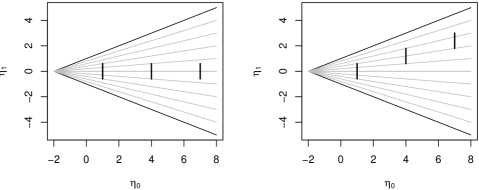
Figure 1: Prior parameter set $\mathrm{H}^{(0)}=\eta_{0}^{(0)}\times[\text{\text@underline{$\eta$}${}_{1}^{(0)}$},\overline{\eta}_{1}^{(0)}]$ and respective posterior sets $\mathrm{H}^{(n)}$ for $s/n=0.5$ (left) and $s/n=0.9$ (right). Bounds for the domain $\mathrm{H}$ are in black, with rays of constant expectation for $y_{c}=\{0.1,0.2,\ldots,0.9\}$ in grey. Note that all sets have the same size, imprecision decreasing only through their position on the $\eta_{0}$ axis.

For prior-data conflict sensitivity, we need sets $\mathrm{H}^{(0)}$ that cover a range of $\eta_{0}$ values, just like sets $I\!\!\Pi^{(0)}$ with a range of $n^{(0)}$ values are necessary to ensure this property. A set $\mathrm{H}^{(0)}$ that is elongated along a certain ray of constant expectation will behave similar to a rectangular $I\!\!\Pi^{(0)}$. When shifted along its ray of constant expectation, imprecision will be reduced as the shadow of $\mathrm{H}^{(0)}$ will become smaller just as described above for line segments. When $\mathrm{H}^{(0)}$ is instead shifted away from its ray of constant expectation, imprecision will increase, as a prolonged shape that is now turned away from its ray will cast a larger shadow.

4 The Boatshape

The shape for $\mathrm{H}^{(0)}$ that we suggest to obtain both prior-data conflict sensitivity and reduced imprecision in case of strong prior-data agreement looks like a boat with a transom stern (see Fig. 2 below). The curvature along its length in the direction of its constant rays of expectation leads to smaller $\Delta_{y}(I\!\!\Pi^{(n)})$ as compared to a rectangular $I\!\!\Pi^{(0)}$ with the same prior range $\Delta_{y}(I\!\!\Pi^{(0)})$, see Fig. 3. The strong prior-data agreement effect is realized through the touchpoints determining $\underline{y}^{(n)}_{\mathrm{H}}$ and $\overline{y}^{(n)}_{\mathrm{H}}$ moving along the shape during updating, see Sect. 4.2. This is advantageous since the spread of the Beta posteriors is determined by $\eta_{0}=n^{(0)}-2$. In case of strong prior-data agreement, variances in the ‘critical’ distributions at the boundary of the posterior expectation interval $[\underline{y}^{(n)}_{\mathrm{H}},\overline{y}^{(n)}_{\mathrm{H}}]$ will thus be lower leading to reduced imprecision.

4.1 Basic Definition

We suggest an exponential function for the contours of a boat-shaped parameter set $\mathrm{H}^{(0)}$. We first restrict discussion on prior sets that are symmetric to the $\eta_{0}$ axis, i.e., centered around $y_{c}=0.5$. Sets $\mathrm{H}^{(0)}$ with central ray $y_{c}\neq 0.5$ can be obtained by rotating the set around $(\eta_{0},\eta_{1})=(-2,0)$ such that $y_{c}$ forms the axis of symmetry. Results for sets with $y_{c}=0.5$ generalize straightforwardly to the case $y_{c}\neq 0.5$; an example is given in Fig. 6. The lower and the upper contour functions are defined as

$$\underline{c}^{(0)}(\eta_{0}) =-a\left(1-e^{-b(\eta_{0}-\underline{\eta}_{0})}\right)\,, \overline{c}^{(0)}(\eta_{0}) =a\left(1-e^{-b(\eta_{0}-\underline{\eta}_{0})}\right)\,,$$ (7)

where $a>0$ and $b>0$ are parameters controlling the shape of $\mathrm{H}^{(0)}$, which is defined as

$$\mathrm{H}^{(0)}=\{(\eta_{0},\eta_{1})\colon\underline{\eta}_{0}\leq\eta_{0}\leq\overline{\eta}_{0},\underline{c}^{(0)}(\eta_{0})\leq\eta_{1}\leq\overline{c}^{(0)}(\eta_{0})\}\,.$$ (8)

A prior boatshape set, together with corresponding posterior sets for different observations, is shown in Fig. 2. The same prior and posterior sets in terms of $(n^{(0)},y^{(0)})$ are depicted in Fig. 3.

Figure 2: Boatshape prior and posterior sets for data in accordance and in conflict with the prior set. The parameters for the prior set are $\underline{\eta}_{0}=1$, $\overline{\eta}_{0}=6$, $a=1.5$, and $b=0.9$. While the posterior sets for $\frac{s}{n}=0.5$ move along the ray for $y_{c}=0.5$, the posterior sets for $\frac{s}{n}=1$ are shifted away from the ray for $y_{c}=0.5$, resulting in increased posterior imprecision. Note that lower and upper touchpoints are in the middle of the contour for the prior set and the posterior sets resulting for data $\frac{s}{n}=0.5$, while the lower touchpoint is at the end for the posterior sets for data $\frac{s}{n}=1$.

The parameter $a$ determines the half-width of the set; the size in the $\eta_{1}$ dimension would be $2a$ if $\overline{\eta}_{0}\to\infty$. Parameter $b$ determines the ‘bulkyness’ of the shape. Together with $\underline{\eta}_{0}$, $a$ and $b$ determine $[\underline{y}^{(0)}_{\mathrm{H}},\overline{y}^{(0)}_{\mathrm{H}}]$. Decreasing $\underline{\eta}_{0}$, or increasing $a$ or $b$, leads to a wider $[\underline{y}^{(0)}_{\mathrm{H}},\overline{y}^{(0)}_{\mathrm{H}}]$. $\overline{\eta}_{0}$ plays only a role in determining when the ‘unhappy learning’ phase starts (see end of Sect. 4.3).

Figure 3: Boatshape prior and posterior sets from Fig. 2 in the $(n^{(0)},y^{(0)})$ parametrization. The rectangular prior set with the same range for $y^{(0)}$ as the prior boatshape set and the corresponding posterior sets are drawn with dashed lines. Unions of symmetric credibility intervals ($\gamma=0.5$) are drawn as vertical bars. Note that all posterior boatshape sets have shorter $y^{(n)}$ ranges than their corresponding posterior rectangle sets, and boatshape credibility regions are especially short for posterior sets where $\frac{s}{n}=0.5$.

We see from the prior set in Fig. 3 that the lower and the upper bound for $y^{(0)}$ is attained in the middle of the set contour. To determine $\underline{y}^{(0)}_{\mathrm{H}}$ and $\overline{y}^{(0)}_{\mathrm{H}}$, we need to find the corresponding touchpoints ${\eta_{0}^{l}}{}^{(0)}$ and ${\eta_{0}^{u}}{}^{(0)}$ by identifying the rays of constant expectation that are tangents to $\mathrm{H}^{(0)}$ and then solving for $\eta_{0}$. Since $\mathrm{H}^{(0)}$ is symmetric to the $\eta_{0}$ axis, we have ${\eta_{0}^{l}}{}^{(0)}={\eta_{0}^{u}}{}^{(0)}$ and we will determine ${\eta_{0}^{u}}{}^{(0)}$ by considering the upper contour tangent. We get

$$1+b({\eta_{0}^{u}}{}^{(0)}+2) \stackrel{{\scriptstyle!}}{{=}}e^{b({\eta_{0}^{u}}{}^{(0)}-\underline{\eta}_{0})}\,.$$ (9)

This equation only has one solution for ${\eta_{0}^{u}}{}^{(0)}>\underline{\eta}_{0}$ that is, however, not available in closed form. Generally, the nearer ${\eta_{0}^{u}}{}^{(0)}$ is to $\underline{\eta}_{0}$, the larger $\frac{d}{d\eta_{0}}\overline{c}^{(0)}({\eta_{0}^{u}}{}^{(0)})$, such that $\overline{y}^{(0)}_{\mathrm{H}}$ is further away from $\frac{1}{2}$.

4.2 Strong Prior-Data Agreement Property

Sets (8) lead to reduced imprecision in inferences when data are strongly supporting prior information as the touchpoint moves further to the right in that case. The basic shape is symmetric around the $\eta_{0}$ axis ($\mathrm{H}^{(0)}$ has central ray $y_{c}=0.5$), and updating with strong-agreement data $s/n=0.5$ means that $\mathrm{H}^{(0)}$ is shifted along the $\eta_{0}$ axis by $n$, such that also $\mathrm{H}^{(n)}$ is symmetric around the $\eta_{0}$ axis. We thus need to consider only one touchpoint. Movement to the right means that the upper posterior touchpoint ${\eta_{0}^{u}}{}^{(n)}$ is larger than the updated prior touchpoint ${\eta_{0}^{u}}{}^{(0)}$, so we need to show that ${\eta_{0}^{u}}{}^{(n)}>{\eta_{0}^{u}}{}^{(0)}+n$. The upper contour for the posterior boatshape, updated with $s=\frac{n}{2}$, is $\overline{c}^{(0)}$ from (7) shifted to the right by $n$, i.e., $\overline{c}^{(n)}(\eta_{0})=a-ae^{-b(\eta_{0}-n-\underline{\eta}_{0})}$. The equation to identify the posterior upper touchpoint is

$$1+b({\eta_{0}^{u}}{}^{(n)}+2) \stackrel{{\scriptstyle!}}{{=}}e^{b({\eta_{0}^{u}}{}^{(n)}-n-\underline{\eta}_{0})}\,.$$ (10)

Comparing (10) to (9), both have a linear function with slope $b$ and intercept $1+2b$ on the left hand side. The exponential function on the right hand side of (10) is the function on the right hand side of (9) shifted to the right by $n$. We can picture this situation as in Fig. 4: ${\eta_{0}^{u}}{}^{(0)}$ is identified by the intersection of the linear function with the left, non-shifted exponential, whereas ${\eta_{0}^{u}}{}^{(n)}$ is at the intersection of the linear function with the right, shifted exponential. Since $b>0$, we have indeed ${\eta_{0}^{u}}{}^{(n)}>{\eta_{0}^{u}}{}^{(0)}+n$.

Figure 4: Illustration for the argument that ${\eta_{0}^{u}}{}^{(n)}>{\eta_{0}^{u}}{}^{(0)}+n$.

4.3 Touchpoints for Arbitrary Updates

Let us now consider the update of the basic boatshape (8) in the general case $s\neq\frac{n}{2}$, investigating the effect that different values of $s$ for fixed $n$ have on ${\eta_{0}^{l}}{}^{(n)}$ and ${\eta_{0}^{u}}{}^{(n)}$ For $s\neq\frac{n}{2}$, $\mathrm{H}^{(n)}$ is not symmetric to the $\eta_{0}$ axis, and we have to derive the touchpoints ${\eta_{0}^{l}}{}^{(n)}$ and ${\eta_{0}^{u}}{}^{(n)}$ separately. The upper and lower contours for $\mathrm{H}^{(n)}$ are

$$\overline{c}^{(n)}(\eta_{0}) =s-\frac{n}{2}+a-ae^{-b(\eta_{0}-n-\underline{\eta}_{0})}\,, \underline{c}^{(n)}(\eta_{0}) =s-\frac{n}{2}-a+ae^{-b(\eta_{0}-n-\underline{\eta}_{0})}\,,$$

leading to

$$\frac{a}{s-\frac{n}{2}+a}\big{(}1+b({\eta_{0}^{u}}{}^{(n)}+2)\big{)} \stackrel{{\scriptstyle!}}{{=}}e^{b({\eta_{0}^{u}}{}^{(n)}-n-\underline{\eta}_{0})}\,,$$ (11)

$$\frac{a}{\frac{n}{2}-s+a}\big{(}1+b({\eta_{0}^{l}}{}^{(n)}+2)\big{)} \stackrel{{\scriptstyle!}}{{=}}e^{b({\eta_{0}^{l}}{}^{(n)}-n-\underline{\eta}_{0})}\,.$$ (12)

We see that the graph from Fig. 4 holds here as well, except that the linear function on the left hand side of (11) and (12) is changed in slope and intercept by a factor. (Equivalently, we can consider it to be rotated around the root $-2-\frac{1}{b}$.) For $s=\frac{n}{2}$, this factor is 1 for both (11) and (12), reducing to (10). Due to symmetry of $\mathrm{H}^{(0)}$ we consider, without loss of generality, only the case $s>\frac{n}{2}$.

The factor $\frac{a}{s-\frac{n}{2}+a}$ in (11) is smaller than $1$ and decreasing in $s$ to $\frac{a}{\frac{n}{2}+a}$ for $s=n$. As the linear function’s slope will be less steep (the intercept is lowered as well), the intersection with the exponential function moves to the left, i.e. ${\eta_{0}^{u}}{}^{(n)}(s)<{\eta_{0}^{u}}{}^{(n)}(\frac{n}{2})$ for $\frac{n}{2}<s<n$. This means that $\overline{y}^{(n)}_{\mathrm{H}}(s)>\overline{y}^{(n)}_{\mathrm{H}}(\frac{n}{2})$. However, ${\eta_{0}^{u}}{}^{(n)}(s)$ can decrease only to $\underline{\eta}_{0}+n$: When ${\eta_{0}^{u}}{}^{(n)}(s)$ reaches the left end of $\mathrm{H}^{(n)}$ at $\underline{\eta}_{0}+n$, the gradual increase of $\overline{y}^{(n)}_{\mathrm{H}}$ through the changing tangent slope is replaced by a different change mechanism, where increase of $\overline{y}^{(n)}_{\mathrm{H}}$ is solely due to the shift of $\mathrm{H}^{(n)}$ in the $\eta_{1}$ coordinate. Due to (4), $\overline{y}^{(n)}_{\mathrm{H}}$ is then linear in $s$.

In (12), the factor to the linear function is $\frac{a}{\frac{n}{2}-s+a}$. Here, we have to distinguish the two cases $\frac{n}{2}\leq s<\frac{n}{2}+a$ and $s\geq\frac{n}{2}+a$. In the first case, the factor is larger than $1$ and increasing in $s$ so the intersection of the linear function with the exponential function will move to the right, such that ${\eta_{0}^{l}}{}^{(n)}(s)$ becomes larger, and $\underline{y}^{(n)}_{\mathrm{H}}$ increases. In the second case, the factor is undefined (for $s=\frac{n}{2}+a$) or negative (for $s>\frac{n}{2}+a$) and there is no intersection of the linear function with the exponential function for any $\eta_{0}>\underline{\eta}_{0}+n$. So for $s\geq\frac{n}{2}+a$, the whole set is above the $\eta_{0}$ axis, and the touchpoint must thus be at $\overline{\eta}_{0}+n$. Actually, ${\eta_{0}^{l}}{}^{(n)}(s)=\overline{\eta}_{0}+n$ already for some $\frac{n}{2}\leq s<\frac{n}{2}+a$, when the intersection point reaches $\overline{\eta}_{0}+n$. At this point, gradual increase of $\underline{y}^{(n)}_{\mathrm{H}}$ resulting from the movement of ${\eta_{0}^{l}}{}^{(n)}(s)$ along the set towards the right is replaced by a linear increase in $s$. Again, this is because the $\eta_{1}$ coordinate is incremented according to (6), and from (4) we see that $\underline{y}^{(n)}$ is linear in $\eta_{1}$.

4.4 Posterior Imprecision

We now summarize the results from Sect. 4.3 and give two numerical examples. For $s>\frac{n}{2}$, both $\overline{y}^{(n)}$ and $\underline{y}^{(n)}$ will at first increase gradually with $s$, as ${\eta_{0}^{u}}{}^{(n)}$ moves to the left, and ${\eta_{0}^{l}}{}^{(n)}$ moves to the right. We will call such updating of the prior parameter set, where both lower and upper posterior touchpoints are in the middle of the set, happy learning.

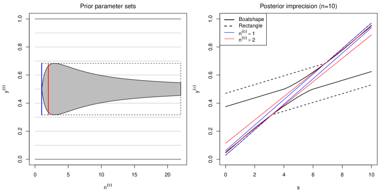
Figure 5: Boatshape set with $y_{c}=0.5$ together with rectangle set, $1\times[\underline{y}^{(0)},\overline{y}^{(0)}]$ and $2\times[\underline{y}^{(0)},\overline{y}^{(0)}]$ with same prior imprecision (left), and the corresponding lower and upper bounds for $y^{(n)}$ as functions of $s$ (right).

At some $s^{u}$, ${\eta_{0}^{u}}{}^{(n)}$ will reach $\underline{\eta}_{0}+n$, and at some $s^{l}$, ${\eta_{0}^{l}}{}^{(n)}$ will reach $\overline{\eta}_{0}+n$. Whether $s^{l}<s^{u}$ or vice versa depends on the choice of parameters $\underline{\eta}_{0},\overline{\eta}_{0},a$ and $b$. When $s$ is larger than either $s^{l}$ or $s^{u}$, we have unhappy learning, where data $s$ is very much out of line with our prior expectations as expressed by $\mathrm{H}^{(0)}$. Ultimately, when $s>s^{u}$ and $s>s^{l}$, both $\overline{y}^{(n)}_{\mathrm{H}}$ and $\underline{y}^{(n)}_{\mathrm{H}}$ will increase linearly in $s$, but with different slopes. $\overline{y}^{(n)}_{\mathrm{H}}$ will increase with slope $\frac{1}{\underline{\eta}_{0}+n+2}$, whereas $\underline{y}^{(n)}_{\mathrm{H}}$ will increase with the lower slope $\frac{1}{\overline{\eta}_{0}+n+2}$.

These findings are illustrated in Fig. 5 for a boatshape set with $y_{c}=0.5$, $\underline{\eta}_{0}=-1$, $\overline{\eta}_{0}=20$, $a=1$ and $b=0.4$. These are compared to a rectangular set and two line segment sets with the same $y^{(0)}$ range. Here we see a linear increase of $\overline{y}^{(n)}_{\mathrm{H}}$ for $s<4$ and a superlinear increase for $s\geq 4$. We have happy learning for $s\in[4,6]$, and unhappy learning for $s\neq[4,6]$. For $s\approx 5$, $\Delta_{y}$ for the boatshape set is about half of $\Delta_{y}$ for the rectangle set. The line segment sets lead to very short $y^{(n)}$ ranges, but do not reflect prior-data conflict.

Figure 6 depicts a numerical example for the case $y_{c}=0.75$. Notice that the rotated boatshape parameter set is not symmetric in the $(n^{(0)},y^{(0)})$ space. We see that $[\underline{y}^{(n)}_{\mathrm{H}},\overline{y}^{(n)}_{\mathrm{H}}]$ is nearly as short as $[\underline{y}^{(n)},\overline{y}^{(n)}]$ for the line segments sets when $s\approx 0.75$, but that unlike those, the boatshape offers prior-data conflict sensitivity. Interestingly, all four sets lead to a similar $\underline{y}^{(n)}$ for $s<5$.

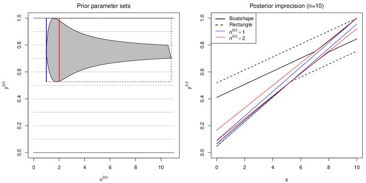
Figure 6: Boatshape set with $y_{c}=0.75$ together with rectangle set, $1\times[\underline{y}^{(0)},\overline{y}^{(0)}]$ and $2\times[\underline{y}^{(0)},\overline{y}^{(0)}]$ with same prior imprecision (left), and the corresponding lower and upper bounds for $y^{(n)}$ as functions of $s$ (right).

5 Concluding Remarks

For application of the novel method presented in this paper, elicitation of the boatshape set parameters must be considered, pre-posterior analysis seems useful for this. It will be interesting to investigate whether another way of defining a set aligned to a certain ray could be useful, namely by shifting each part of $\mathrm{H}^{(0)}$ from (8) in the $\eta_{1}$ dimension onto the desired ray (similar to turning a right prism into an oblique prism). Alternatives to the functional form of the contour functions (7) could also be worth of study. The method was presented here for the case of binary data, it can be easily generalized to cover all sample distributions that belong to the exponential family, since for those a conjugate prior in the $(\eta_{0},\eta_{1})$ parametrization can be constructed having a purely data-dependent translation as update step [3, p. 56].

In the parameter space described in Sect. 3, updating the prior set amounts to a purely data-dependent translation, leaving the set shape unchanged. As shown, this enables flexible modeling of prior information and tailored posterior inference properties, while remaining within the generalized Bayesian paradigm, hence opening a wide field of research on prior set shapes for specific inference objectives.

5.0.1 Acknowledgements

Gero Walter was supported by the Dinalog project “Coordinated Advanced Maintenance and Logistics Planning for the Process Industries” (CAMPI).

References

- [1] Augustin, T., Coolen, F., de Cooman, G., Troffaes, M.: Introduction to Imprecise Probabilities. Wiley, Chichester (2014)
- [2] Berger, J. et al.: An overview of robust Bayesian analysis. TEST 3, 5–124 (1994)
- [3] Bickis, M.: The geometry of imprecise inference. In: Augustin, T., Doria, S., Miranda, E., Quaeghebeur, E. (eds.) ISIPTA ’15: Proceedings of the Ninth International Symposium on Imprecise Probability: Theories and Applications, pp. 47–56. SIPTA (2015), http://www.sipta.org/isipta15/data/paper/31.pdf
- [4] Evans, M., Moshonov, H.: Checking for prior-data conflict. Bayesian Analysis 1, 893–914 (2006), http://projecteuclid.org/euclid.ba/1340370946
- [5] Quaeghebeur, E., de Cooman, G.: Imprecise probability models for inference in exponential families. In: Cozman, F., Nau, R., Seidenfeld, T. (eds.) ISIPTA ’05. Proceedings of the Fourth International Symposium on Imprecise Probabilities and Their Applications. pp. 287–296. SIPTA, Manno (2005)
- [6] Robert, C.P.: The Bayesian Choice: From Decision-Theoretic Foundations to Computational Implementation. Springer, New York (2007)
- [7] Troffaes, M., Walter, G., Kelly, D.: A robust Bayesian approach to modelling epistemic uncertainty in common-cause failure models. Reliability Engineering & System Safety 125, 13–21 (2014), http://dx.doi.org/10.1016/j.ress.2013.05.022
- [8] Walley, P.: Statistical Reasoning with Imprecise Probabilities. Chapman and Hall, London (1991)
- [9] Walley, P.: Inferences from multinomial data: Learning about a bag of marbles. Journal of the Royal Statistical Society, Series B 58(1), 3–34 (1996)
- [10] Walter, G.: Generalized Bayesian inference under prior-data conflict. Ph.D. thesis, Ludwig-Maximilians-Universität München (2013), http://nbn-resolving.de/urn:nbn:de:bvb:19-170598
- [11] Walter, G., Augustin, T.: Imprecision and prior-data conflict in generalized Bayesian inference. Journal of Statistical Theory and Practice 3, 255–271 (2009)
- [12] Walter, G., Graham, A., Coolen, F.P.A.: Robust Bayesian estimation of system reliability for scarce and surprising data. In: Podofillini, L., Sudret, B., Stojadinović, B., Zio, E., Kröger, W. (eds.) Safety and Reliability of Complex Engineered Systems: ESREL 2015, pp. 1991–1998. CRC Press (2015)