Temporal steering in four dimensions with applications to coupled qubits and magnetoreception.

Abstract

Einstein-Podolsky-Rosen (EPR) steering allows Alice to remotely prepare a state in some specific bases for Bob through her choice of measurements. The temporal analog of EPR steering, temporal steering, also reveals the steerability of a single system between different times. Focusing on a four-dimensional system, here we investigate the dynamics of the temporal steering measures, the temporal steering robustness, using five mutually unbiased bases. As an example of an application, we use these measures to examine the temporal correlations in a radical pair model of magneto-reception. We find that, due to interactions with a static nuclear spin, the radical pair model exhibits strong non-Markovianity.

I introduction

Quantum steering Schrödinger (1935); Reid (1989); Wiseman et al. (2007); Cavalcanti et al. (2009) is an intriguing phenomenon wherein one party can remotely steer the quantum state of another party through their choice of measurements. Remarkably, there exists a hierarchy relation between steering, Bell nonlocality, and entanglement. That is, states which are Bell nonlocal are also steerable, and all steerable states are entangled, but not vice versa Wiseman et al. (2007); Quintino et al. (2015). Numerous applications of steering have been considered, such as the connection to one-side device independent quantum key distribution Branciard et al. (2012); Gallego and Aolita (2015), a geometrical representation of steering Jevtic et al. (2014), the correspondence with measurement incompatibility Uola et al. (2014); Quintino et al. (2014); Uola et al. (2015), steering beyond quantum theory Sainz et al. (2015), multipartite steering Armstrong et al. (2015); Li et al. (2015a); Cavalcanti et al. (2015), etc. In addition, there have been many efforts at quantifying steering Skrzypczyk et al. (2014); Piani and Watrous (2015); Kogias et al. (2015); Gallego and Aolita (2015); Costa and Angelo (2016); Cavalcanti and Skrzypczyk (2016). In addition, many experiments exhibiting the reality of steering have also been performed Wittmann et al. (2012); Smith et al. (2012); Saunders et al. (2010); Li et al. (2015a).

A range of different types of quantum correlations also appear when measuring a single system at different times. For example, the Leggett-Garg (LG) inequality Leggett and Garg (1985); Emary et al. (2014), a temporal analog of Bell’s inequality, based on the assumption of macroscopic realism, relies on combining two-time correlation functions Emary et al. (2012); Lambert et al. (2010). Similarly, other types of temporal correlations have been proposed and investigated, including quantum entanglement in time, temporal nonlocality, and bounding temporal quantum correlations Brukner et al. (2004); Fritz (2010); Budroni et al. (2013); Budroni and Emary (2014). Motivated by the correspondence between Bell’s nonlocality and the LG inequality, a temporal analog of steering was proposed by Chen et al. Chen et al. (2014, 2016); Li et al. (2015b). Focusing on a single system transmitted from Alice to Bob, temporal steering demonstrates Alice’s influence on Bob via her choice of measurements. Temporal steering is related to quantum key distribution Chen et al. (2014, 2016); Bartkiewicz et al. (2016b); Li et al. (2015b), measurement incompatibility Karthik et al. (2015), and quantum non-Markovianity Chen et al. (2016). The first experiment showing temporal steering has also recently been reported by Bartkiewicz et al. Bartkiewicz et al. (2016a).

Although some works concerning temporal steering have been proposed, research on temporal steering in higher dimensions is still lacking. Here, we introduce a new quantifier, temporal steering robustness, in analogy with spatial steering robustness Piani and Watrous (2015). Then, we move on to considering the temporal steering robustness of four dimensional systems. As examples, we first consider two coupled qubits, and construct its temporal assemblage using five mutually unbiased bases (MUBs) Klappenecker and Roetteler (2003). Second, we consider the radical-pair model, a “toy model” used to describe the sensitivity of certain chemical reactions to magnetic fields, and which is one of the candidate models for the origin of avian magnetoreception. Finally, we investigate the non-Markovianity of the dynamics of electrons in the radical pair model, as revealed by nonmonotonic temporal steering.

II Temporal steering and how to quantify it

II.1 Formulation of temporal steering

First, let us briefly review the concept of temporal steering. Alice performs a measurement, which can be described by a set of positive-operator valued measures (POVMs) $\{E_{a|x}\}$, with measurement choice $x$ on an initial state $\rho_{0}$ at time $t=0$. After the measurement, she obtains an outcome $a$ and a postmeasurement state $\hat{\sigma}_{a|x}(t=0)=M_{a|x}\rho_{0}M^{\dagger}_{a|x}/p(a|x)$, where $p(a|x)=\text{tr}(M_{a|x}\rho_{0}M^{\dagger}_{a|x})$, with $M^{\dagger}_{a|x}M_{a|x}=E_{a|x}$. After that Alice sends the state $\hat{\sigma}_{a|x}(t=0)$ to Bob through a quantum channel $\Lambda$, in which a unitary evolution or environment-induced noise may take place. After the transmission, Bob receives the assemblage $\hat{\sigma}_{a|x}(t)=\Lambda[\hat{\sigma}_{a|x}(t=0)]$ at time $t$.

To verify whether Alice’s choice of measurement influences Bob’s received state, Bob checks whether the assemblage ${\sigma}_{a|x}(t):=p(a|x)\sigma_{a|x}(t)$ can be written in a hidden-state form:

$$\sigma_{a|x}(t)~{}=~{}\sigma_{a|x}^{\textrm{T,US}}~{}=~{}\sum_{\lambda}P(\lambda)~{}P(a|x,\lambda)~{}\sigma_{\lambda}.$$ (1)

If it is the case, Bob would think that the probability distribution $P(\lambda)$ can be reconstructed from Alice’s measurement setting $x$ and the outcome $a$. In addition, he would also think that the states he receives are predetermined by $\sigma_{\lambda}$ during each round of the experiment, and not actually influenced by Alice’s measurement choice. Thus all Alice has to do is use her knowledge of the probability distribution $\lambda$ and $P(a|x,\lambda)$ to construct her measurement results. What Bob receives is the statistical average of the state of Eq. (1). Conversely, if it is not the case that his assemblage can be written in a hidden-state form, he convinces himself that the state he receives is actually influenced by Alice’s choice of measurement.

In Ref. Piani and Watrous (2015), Piani and Watrous introduced a quantifier of steering — steering robustness, the minimum noise needed to destroy the steerability of the assemblage. Here, we show that there also exists a temporal analog of steering robustness — temporal steering robustness (TSR), that can serve as a quantifier of temporal steering.

Similar to the steering robustness, the temporal steering robustness is defined as the minimum noise needed to destroy the temporal steerability of the temporal assemblage:

$$\text{TSR}:=\text{min}{}{} t\geq 0$$ (2)

subject to $$\left\{\frac{\sigma_{a|x}^{\text{T}}+t~{}\tau_{a|x}}{1+t}\right\}_{a,x}~{}~{}\text{temporal unsteerable},$$

$$\{\tau_{a|x}\}_{a,x}:\text{an assemblage}.$$

Following the procedure in Ref. Piani and Watrous (2015), the condition (2) can also be written as an semidefinite programming (SDP) optimization problem:

$$\text{TSR}=\text{min}{}{} \text{tr}\sum_{\lambda}\sigma_{\lambda}-1$$ (3)

subject to $$\sum_{\lambda}D_{\lambda}(a|x)\sigma_{\lambda}\geq\sigma_{a|x}~{}~{} \forall~{}a,x$$

$$\sigma_{\lambda}\geq 0 \forall~{}\lambda,$$

where $\sigma_{\lambda}=(1+t)\sigma^{\textrm{T},\text{US}}_{a|x}$ and $D_{\lambda}(a|x)=\delta_{a,\lambda(x)}$ Chen et al. (2016); Skrzypczyk et al. (2014) is the deterministic value of the single-party conditional probability distributions $P(a|x,\lambda)$. In the following section, we will use the temporal steering robustness to realize the temporal correlation in higher-order system for some specific quantum channel.

III Temporal Steering in Systems with Dimension $\bm{d=4}$

III.1 Two qubits coherently coupled with each other

In this section, we examine the dynamics of the temporal steerability of a system composed of two qubits coherently coupled with each other, given by the interaction Hamiltonian $H=g(\sigma_{1}^{+}\sigma_{2}^{-}+\sigma_{1}^{-}\sigma_{2}^{+})$, where $g$ is the coupling strength between the two qubits, and $\sigma_{i}^{+}$ and $\sigma_{i}^{-}$ are the raising and lowering operators of the $i$th qubit, respectively. In addition, each qubit is subject to a Markovian decay process. The evolution of the entire system is expressed by the master equation with Lindblad form Lindblad (1976)

$$\dot{\rho}=\frac{1}{i\hbar}[H,\rho]+\sum_{i=1}^{2}\frac{\gamma}{2}(2\sigma_{i}^{-}\rho\sigma_{i}^{+}-\sigma_{i}^{+}\sigma_{i}^{-}\rho-\rho\sigma_{i}^{+}\sigma_{i}^{-}),$$ (4)

where $\gamma$ is the decay rate. Mathematically, we can treat the two qubits as a single four-dimensional system, i.e., $|gg\rangle\equiv|1\rangle,~{}~{}|ge\rangle\equiv|2\rangle,~{}~{}|eg\rangle\equiv|3\rangle$, and $|ee\rangle\equiv|4\rangle$, for which the maximum number of MUBs measurement is five. The set of $5$ MUBs is denoted by $M_{a|x}=|\phi_{a|x}\rangle\langle\phi_{a|x}|$ Wiesniak et al. (2011), as detailed in Appendix A.

We assume that the initial state of the two-qubit system is the maximally-mixed state $\rho(0)=\openone/4$, where $\openone$ is the identity matrix. The postmeasurement state $\sigma_{a|x}(t)=M_{a|x}\rho(0)M_{a|x}/p(a|x)$ can be obtained straightforwardly. Figure 1 shows the dynamics of the temporal steering robustness with two measurement settings ($n=2$ and choosing the measurement settings $x=1,2$) with different decay rates $\gamma$. In Fig. 2, we compare the dynamics of temporal steering robustness for different numbers of measurement settings ($n=2$ to $n=5$, and choosing the measurement setting $x=1,...,n$ for each curve). We can see that the temporal steering robustness increases when the number of measurement settings increases, as expected from the original definition of the temporal steering robustness in Eq. (3).

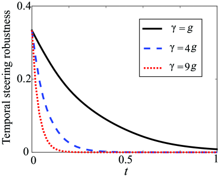
Figure 1: (Color online) The dynamics of temporal steering robustness (two measurement settings) for two coherently coupled qubits with different decay rates $\gamma$. The black-solid, blue-dashed, and red-dotted curves represent $\gamma=g,4g,$ and $9g$, respectively. Here, $t$ is in units of $\gamma^{-1}$. The initial state is in the maximally-mixed state $\rho(0)=\openone/4$.

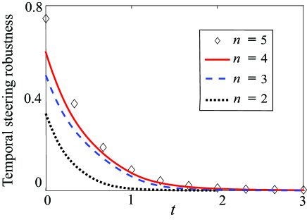
Figure 2: The dynamics of temporal steering robustness of two qubits with different numbers of measurement settings $n$. The decay rate is set as $\gamma=g$, and the initial state is in the maximally-mixed state $\rho(0)=\openone/4$. Here, we compare the results of four kinds of measurement settings ($n=2$ to $5$). For example, when $n=3$, $\{M_{a|x}\}=\{M_{a|1},M_{a|2},M_{a|3}\}$. We see that the temporal steering robustness increases with the number of measurement settings, due to the intrinsic definition of the measure of (temporal) steerability Skrzypczyk et al. (2014); Piani and Watrous (2015); Chen et al. (2016).

III.2 Temporal Steering Robustness of the Radical Pair

The mechanism by which birds and other animals navigate using the geomagnetic field is still unclear. Among various proposals, the radical-pair model has received considerable attention due to its ability to predict many of the behavioral features seen in experiments and its uniquely quantum features Gauger et al. (2011). In addition, radical-pair reactions are known to occur within the biological photoreceptor cryptochrome Mouritsen et al. (2004); Moller et al. (2004), perhaps leading to a biologically detectable signal. In the traditional “toy-model” of this process, a radical pair within or attached to the cryptochrome is formed when an electron is excited from a donor to a receptor molecule, which thus hosts spatially-separated electrons in a spin-singlet or triplet state. The electron pair then evolves coherently between these states, under the influence of the geomagnetic field and the hyperfine interactions with the host nuclei Ritz et al. (2010); Lambert et al. (2013a). At a later time, the singlet-triplet conversion leads to different chemical reaction products that could lead to a biologically-detectable signal. Figure 3 depicts the basic concept of the radical-pair model. Of course, in reality the chemical-process may be much more complicated than this toy-model suggests, but it is helpful to consider such a model because of its simplicity and intuitive ability to explain some behaviorial features. Despite this simplicity, here we find that the analysis of higher-dimensional steering in this model reveals some surprising and counterintuitive features.

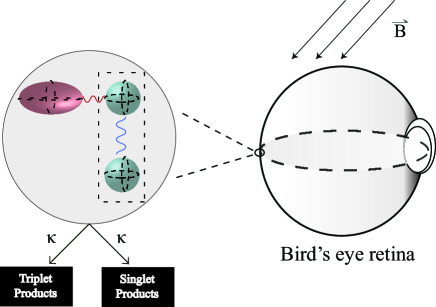
Figure 3: (Color online) Schematic diagram of the radical-pair model. The radical-pair mechanism for avian navigation can explain some of the features of behavioral experiments of European robins Gauger et al. (2011); Moller et al. (2004); Ritz et al. (2010). It is thought that it may occur within certain cryptochrome proteins residing in the eye. The simplest radical-pair toy-model is composed of two electrons and a nucleus, coupled to one of the electrons with the hyperfine interaction. The singlet and triplet states of the two electrons in the radical pair inter-convert due to a combination of the Zeeman splitting due to the geomagnetic field, and an anisotropic nuclear hyperfine interaction. At later times, the singlet and triplet states decay into chemical products, dependent on their spin nature, which we track with the ancilla shelving states $S$ and $T$, respectively.

The simplest radical-pair model contains two electrons and one nuclear spin Gauger et al. (2011). The nucleus interacts with only one of the electrons, while the other is free. The hyperfine interaction between the nucleus and the electron together with the Zeeman effect induce the interconversion between the singlet and triplet states. For the radical-pair model to be sensitive to the angle of the external geomagnetic field, the hyperfine coupling tensor must be anisotropic. The anisotropic hyperfine tensor between the nuclear spin and electron-1 can be written as $\mathbf{A}=\rm{diag}(\mathrm{A}_{\mathrm{x}},\mathrm{A}_{\mathrm{y}},\mathrm{A}_{\mathrm{z}})$. Here, we consider two kinds of anisotropic hyperfine tensors $\mathrm{A}_{\mathrm{x}}=\mathrm{A}_{\mathrm{y}}=0$, $|\mathrm{A}_{\mathrm{z}}|=10^{5}$ and $\mathrm{A}_{\mathrm{x}}=\mathrm{A}_{\mathrm{y}}=\mathrm{A}_{\mathrm{z}}/2$ with $|\mathrm{A}_{\mathrm{z}}|=10^{5}$ m eV  Gauger et al. (2011); Lambert et al. (2013b); Pauls et al. (2013). The Zeeman effect is included due to the coupling between the magnetic field and the electrons. The Hamiltonian of the entire system is

$$H=\sum_{i=1}^{2}\gamma\mathbf{B}\cdot\mathbf{S}_{i}+\mathbf{I}\cdot\mathbf{A}\cdot\mathbf{S}_{1},$$ (5)

where $\mathbf{S}_{i}\equiv(\sigma_{\mathrm{x},i},\sigma_{\mathrm{y},i},\sigma_{\mathrm{z},i})$ are the electron spin operators ($i=\mathrm{1}$,2) with Pauli matrices $\sigma$, $\mathbf{I}$ is the spin operator for the nucleus, and $\mathbf{B}$ is the magnetic field. Here, $\gamma=\frac{1}{2}\mu_{B}g_{s}$ is the gyromagnetic ratio with $\mu_{B}$ being the Bohr’s magneton and $g_{s}=2$ being the magnetic moment Lambert et al. (2013b). The magnetic field for the two electrons and the nucleus can be generally described by

$$\mathbf{B}=B_{0}(\cos\phi\sin\theta,\sin\phi\sin\theta,\cos\theta),$$ (6)

where $B_{0}$ = 47 $\mu$T is the intensity of the Earth’s magnetic field. Without loss of generality, an axial symmetry is usually assumed: $\phi=0$ and $\theta\in[0,\pi/2]$.

To mimic the process that the singlet and triplet states decay to the chemical compounds, we additionally add two ancilla-shelving systems (called $S$ and $T$) to the Hilbert space to keep track of the population decay into singlet and triplet products, respectively. These are not physical systems but just mathematically convenient to aid in tracking the change in population. One can also adopt other approaches, which are typically more numerically conservative, but here it is convenient as we wish to investigate the temporal dynamics of the electron-spin systems without loss of population, which we can do by tracing out the ancillas. This corresponds to postselecting on populations which have not decayed. Of course, if one cares about the magnitude of a signal corresponding to the decay processes, one should investigate these populations directly.

Later, we will use a master equation with the Lindblad terms to describe the Markovian decay process from the singlet state, as recorded by the ancilla $S$, as well as from the triplet state, as recorded by the ancilla $T$. The bases of every element of our system are as follows: First, the bases of the electron pair are defined as $\{|s\rangle,|t_{0}\rangle,|t_{-1}\rangle,|t_{+1}\rangle\}$, with $|s\rangle$ and $\{|t_{i}\rangle\}_{i=-1,0,1}$ being that singlet and triplet states, respectively. Second, $|\uparrow\rangle$ and $|\downarrow\rangle$ are the bases describing the nuclear-spin states. Finally, $\{|S_{j}\rangle\}$ and $\{|T_{j}\rangle\}$ (where $j=0,1$) are states of the ancilla $S$ and ancilla $T$, respectively, with $j=0$ describing the subspace where the system has not decayed, and $j=1$ the subspace where it has. With the above definitions, we can now define the projection operators as $P_{s,\uparrow}=|s,\uparrow,S_{1},T_{0}\rangle\langle s,\uparrow,S_{0},T_{0}|$, $P_{t_{0},\uparrow}=|t_{0},\uparrow,S_{0},T_{1}\rangle\langle t_{0},\uparrow,S_{0},T_{0}|$, $P_{t_{-1},\uparrow}=|t_{-1},\uparrow,S_{0},T_{1}\rangle\langle t_{-1},\uparrow,S_{0},T_{0}|$, and $P_{t_{+1},\uparrow}=|t_{+1},\uparrow,S_{0},T_{1}\rangle\langle t_{+1},\uparrow,S_{0},T_{0}|$. The projective operators describe the spin-selective recombination into the chemical compounds (ancilla $S$ and ancilla $T$ states). We also consider additional environmental noise described by the standard Lindblad formalism Gauger et al. (2011); Bandyopadhyay et al. (2012). The dynamics of the density matrix is obtained by solving the following master equation

$$\dot{\rho}= \frac{1}{i\hbar}[H,\rho]+\kappa\sum_{i}^{8}\bigg{[}P_{i}\rho P_{i}^{\dagger}-\frac{1}{2}(P_{i}^{\dagger}P_{i}\rho+\rho P_{i}^{\dagger}P_{i})\bigg{]}+$$ (7)

$$\Gamma\sum_{i=1}^{2}\bigg{[}\sigma_{\mathrm{z},i}\rho\sigma_{\mathrm{z},i}^{\dagger}-\frac{1}{2}(\sigma_{\mathrm{z},i}^{\dagger}\sigma_{\mathrm{z},i}\rho+\rho\sigma_{\mathrm{z},i}^{\dagger}\sigma_{\mathrm{z},i})\bigg{]},$$

where $\sigma_{z,i}$ are the Lindblad operators of the two electrons. Here, we assume that all the singlet and triplet recombination operators have the same decay rate $\kappa=10^{4}$ s^-1, and $\Gamma=10^{3}$ s^-1 is the rate of decoherence of each electron. The value $\kappa=10^{4}$ s^-1 is chosen as it is the one thought to explain certain experimental results in which a small oscillating magnetic field can disrupt the European Robins’ ability to navigate Ritz et al. (2004, 2009); Gauger et al. (2011). An implication of these results is that the decoherence time of the radial-pair model could of the order of 100 $\mu$s or more Gauger et al. (2011).

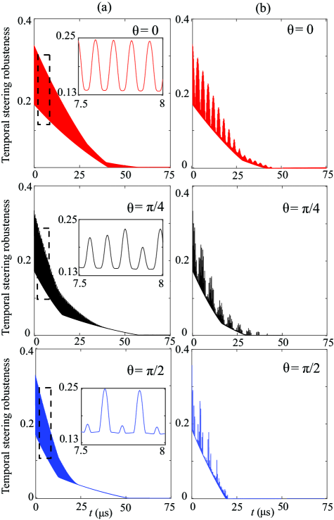
Figure 4: (Color online) The dynamics of temporal steering robustness (two measurement settings, $M_{a|1}$ and $M_{a|2}$) of the radical-pair model. The red, black and blue solid curves represent the results of the angle $\theta=0$, $\theta=\pi/4$, and $\theta=\pi/2$, between the magnetic field and the radical-pair, respectively. In column (a), we set the anisotropic tensor: $\mathrm{A}_{\mathrm{x}}=\mathrm{A}_{\mathrm{y}}=0$, $\mathrm{A}_{\mathrm{z}}=|10^{5}|$ meV Gauger et al. (2011); Lambert et al. (2013b); Pauls et al. (2013). The times when the signals vanish, for the red, black, and blue solid curves curves are $56$ $\mu\textbf{s}$, $53$ $\mu\textbf{s}$, and $50$ $\mu\textbf{s}$ , respectively. In column (b), we set the anisotropic tensor: $\mathrm{A}_{\mathrm{x}}=\mathrm{A}_{\mathrm{y}}=\mathrm{A}_{\mathrm{z}}/2$ with $|\mathrm{A}_{\textrm{z}}|=10^{5}$ meV. The times when the signals vanish, for the red, black and blue solid curves are $45$ $\mu\textbf{s}$, $41$ $\mu\textbf{s}$, and $20$ $\mu\textbf{s}$, respectively. The dynamics of the temporal steering robustness obviously depends on the angle $\theta$ between the magnetic field and the radical-pair in this simplest model.

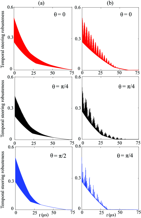
Figure 5: (Color online) The dynamics of temporal steering robustness (three measurement settings, $M_{a|1}$, $M_{a|2}$ and $M_{a|3}$) of the radical-pair model. The red, black, and blue solid curves show the results for the angles $\theta=0$, $\theta=\pi/4$, and $\theta=\pi/2$, between the magnetic field and the radical-pair, respectively. The difference between Fig. 4 and 5 is the number of the measurement settings, $n_{x}$. In column (a), the times when the signals vanish, for the red, black, and blue solid curves are $75$ $\mu\textbf{s}$, $71$ $\mu\textbf{s}$, and $69$ $\mu\textbf{s}$, respectively. In column (b), the times when the signals vanish, for the red, black, and blue solid curves are $62$ $\mu\textbf{s}$, $57$ $\mu\textbf{s}$, and $34$ $\mu\textbf{s}$, respectively.

Previous works Gauger et al. (2011); Pauls et al. (2013); Cai et al. (2010a) have looked at the behavior of the entanglement between the free electron and the electron coupled with the nucleus. Here, we are primarily interested in the temporal quantum correlations of the two-electron system at different times. Also, we assume that the initial state of the entire system (the two electrons, the nuclear spin, and the ancillas $S$ and $T$) is $\rho(t=0^{-})=\frac{1}{8}\times\openone\otimes|S_{0}\rangle\langle S_{0}|\otimes|T_{0}\rangle\langle T_{0}|$, where $\frac{1}{8}\times\openone$ is the maximally-mixed state of the two electrons and nuclear spin Cai et al. (2010a). The five MUBs measurements are performed on the two-qubit system at time $t=0$, producing the temporal state assemblage $\sigma_{a|x}(t)$, and the dynamics of the temporal steering robustness can then be obtained. In Figs. 4 and 5, we plot the dynamics of the temporal steering robustness with two ($n=2$ and choosing the measurement setting $x=1$, 2) and three ($n=3$ and choosing the measurement setting $x=1$, 2, 3) measurement settings, respectively. Here, we can see that the dynamics of the temporal steering robustness is clearly dependent on the orientation $\theta$. While it is hard to state a strong connection between such temporal quantum correlations and the functionality of the avian compass, in the next section we will argue that these results imply a counterintuitive appearance of non-Markovianity in this model, easy to miss without looking at a quantity like the temporal steering robustness.

III.3 The non-Markovianity of the Radical Pair

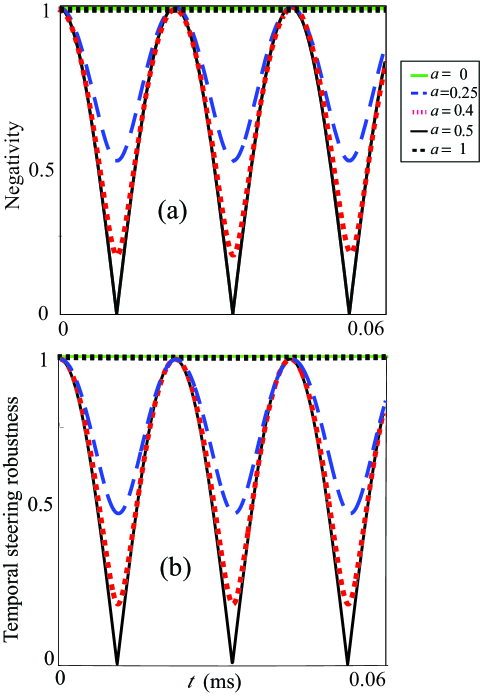
Figure 6: (Color online) The time evolution of the (a) negativity and (b) temporal steering robustness for two electrons of our simplified radical-pair model (i.e., $\Gamma=\kappa=0$). The initial state is a direct product state between the electron singlet state and the nuclear spin state $\rho_{nu}(0)=a\mid\uparrow\rangle\langle\uparrow\mid+(1-a)\mid\downarrow\rangle\langle\downarrow\mid$, with the relative weight $a=0$ (green-solid), $a=0.25$ (blue-dashed), $a=0.4$ (red-dotted), $a=0.5$ (black-solid), and $a=1$ (black-dotted), respectively. When $a=0.25$, $0.4$, and $0.5$, the oscillating curves indicate the non-Markovian nature of the dynamics. In particular, for $a=0.5$, the nuclear spin possesses the largest Shannon entropy and results in the largest oscillation magnitudes in both panels. Consequently, the dynamics of the two electrons shows the strongest non-Markovianity. On the other hand, because $a=0$, $1$, the two electron state evolves unitarily. Hence, the negativity and temporal steering robustness are constant in time.

In Ref. Chen et al. (2016), it was shown that the temporal steerable weight is nonincreasing under completely positive and trace-preserving maps, hence it can be used to define a practical measure of non-Markovianity. Compare Eq. 3 with the SDP formulation of temporal steerable weight in Ref. Chen et al. (2016); it is easy to show that temporal steering robustness can also reveal non-Markovian dynamics. The wavy curves in Figs. 4 and 5 indicate the appearance of non-Markovianity in the radical-pair model. At first this may seem counterintuitive, because the equation of motion is in a Markovian Lindblad form, and, when the hyperfine interaction tensor is $\mathbf{A}=\rm{diag}(0,0,\mathrm{A}_{\mathrm{z}})$, the nuclear-spin polarization remains unchanged during the spin dynamics Cai et al. (2012). However, because the initial state is assumed to be maximally mixed, the electrons effectively experience a mixture of two different evolutions, depending on the nuclear-spin state, leading to the observed non-Markovianity.

TO acquire more insights into this non-Markovianity, we simplify the model by neglecting the decay rate (i.e., $\Gamma=\kappa=0$) and consider the coherent dynamics of the two electrons and nuclear spin. Assuming that the initial state is a direct product state between the electron singlet state and the nuclear-spin state $\rho_{nu}(0)=a|\uparrow\rangle\langle\uparrow|+(1-a)|\downarrow\rangle\langle\downarrow|$. The total density matrix at a later time can be expressed as

$$\rho(t)=a\rho^{1}_{e1,e2}(t)\otimes|\uparrow\rangle\langle\uparrow|+(1-a)\rho^{2}_{e1,e2}(t)\otimes|\downarrow\rangle\langle\downarrow|,$$ (8)

where

$$\rho^{1}_{e1,e2}(t)=\exp[{i\mathrm{A}_{\mathrm{z}}\sigma_{\mathrm{z}}^{1}t}]|s\rangle\langle s|\exp[{-i\mathrm{A}_{\mathrm{z}}\sigma_{\mathrm{z}}^{1}t}]~{}~{}\textrm{and}$$ (9)

$$\rho^{2}_{e1,e2}(t)=\exp[{-i\mathrm{A}_{\mathrm{z}}\sigma_{\mathrm{z}}^{1}t}]|s\rangle\langle s|\exp[{i\mathrm{A}_{\mathrm{z}}\sigma_{\mathrm{z}}^{1}t}],$$

describe the dynamic evolutions of the two electrons under the influence of the magnetic fields locally induced by the nuclear spinors Cai et al. (2012).

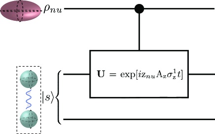
Figure 7: (Color online) Schematic illustration revealing the analogy of our radical-pair model to a controlled-NOT gate. The nuclear spin and two electrons play a role analogous to the control qubit and target qubit, respectively. The nuclear spin state decides the unitary operator $\mathbf{U}=\exp[{i\mathrm{z}_{nu}\mathrm{A}_{\mathrm{z}}\sigma_{\mathrm{z}}^{1}t}]$ exerting on electron 1, where $\mathrm{z}_{nu}=\pm 1$ is the eigenvalue of $\sigma_{\mathrm{z}}$. When $a$ gradually approaches $0.5$, the nuclear spin (C qubit) becomes more uncertain and possesses higher Shannon entropy. Therefore, the non-Markovianity of the two electrons is stronger.

To reveal the non-Markovian nature of the dynamics of the two electrons, we first notice that the state of the two electrons can be expressed as $\rho_{e1,e2}=\mathrm{Tr}_{nu}\rho(t)$. Inspired by the RHP non-Markovianity measure Rivas et al. (2010), in Fig. 6, we show the entanglement of the two electrons quantified by the negativity Życzkowski et al. (1998). When $a=0$ or $1$, the nuclear spin is a pure state in $|\uparrow\rangle$ or $|\downarrow\rangle$, respectively, and the two electron state evolves unitarily. As the nuclear spin becomes a mixed state ($a=0.25$, 0.4, and 0.5), the two electron state is in the form of a convex combination of $\rho_{e1,e2}^{1}(t)$ and $\rho_{e1,e2}^{2}(t)$. Consequently, the time evolution of the entanglement between the two electrons shows oscillations. Therefore, the nuclear spin plays the role of a non-Markovian environment. However, if we consider the entanglement of the nuclear spin and one of the electrons alone, by tracing out the other electron, there is, of course, no entanglement between the nuclear spin and the electron Cubitt et al. (2003).

It is interesting to notice that the non-Markovianity of the convex combination of two unitary transformations, as given by Eq. (8), can be seen as a pair of qubits coupled with each other via a controlled-NOT (CNOT) gate Chen et al. (2015). As shown in Fig. 7, the nuclear spin plays a role analogous to the control qubit (C qubit), which decides the corresponding mixture of unitary operators being exerted on electron 1. It was shown in Ref. (Chen et al., 2015) that when $a$ gradually approaches $0.5$, namely the C qubit becomes more uncertain and possesses higher Shannon entropy, the target qubit exhibits stronger non-Markovianity. This is exactly in line with our results that, as $a$ approaching $0.5$, the oscillation magnitude in Fig. 6 becomes larger, indicating stronger non-Markovianity in the dynamics of the two electrons.

IV CONCLUSION

In summary, we investigate the temporal steering robustness as a mean to quantify temporal steering in high-dimensional systems.To explore its applications, we investigate the dynamics of temporal steering robustness in the radical-pair model. We show that the dynamics of the temporal steering robustness is clearly dependent on the orientation $\theta$. We also reveal the non-Markovianity of the radical-pair model induced by the nuclear spin. The time evolution of the radical pair is the convex combination of two unitary transformations. The different proportions of the nuclear state decide the convex combination of two unitary transformations of the radical pair. When the nuclear spin state is up or down, the dynamics of the system is completely positive and trace-preserving. However, when the nuclear spin is a mixed state, the radical pair behaves non-Markovianly. It is interesting because the nuclear spins are in thermal equilibrium, a completely mixed state. It suggests that non-Markovianity not only plays a role in photosynthesis Lambert et al. (2013a), but may also have some influence in the avian compass.

V APPENDIX

In this appendix, we explicitly give the MUBs which are used as the measurement operators. The MUBs are two orthonormal bases $\{|b_{1}\rangle,...|b_{d}\rangle\}$ and $\{|c_{1}\rangle,...|c_{d}\rangle\}$ of dimensions $d$, such that their complex inner-product between any basis states $|b_{i}\rangle$ and $|c_{j}\rangle$ can be expressed as $|\langle b_{i}|c_{j}\rangle|^{2}=1/d$ Klappenecker and Roetteler (2003). The set of $5$ MUBs is denoted by $\{M_{a|x}\}_{a|x}$, with $a=1$,$2$,$3$,$4$; $x=1$,$2$,$3$,$4$,$5$; and $M_{a|x}=|\phi_{a|x}\rangle\langle\phi_{a|x}|$ where

$$\begin{split}|\phi_{1|1}\rangle&=|1\rangle~{}~{}~{}~{}|\phi_{2|1}\rangle=|2\rangle\\ |\phi_{3|1}\rangle&=|3\rangle~{}~{}~{}~{}|\phi_{4|1}\rangle=|4\rangle\\ \\ |\phi_{1|2}\rangle&=\frac{1}{2}(|1\rangle+|2\rangle+|3\rangle+|4\rangle)\\ |\phi_{2|2}\rangle&=\frac{1}{2}(|1\rangle+|2\rangle-|3\rangle-|4\rangle)\\ |\phi_{3|2}\rangle&=\frac{1}{2}(|1\rangle-|2\rangle-|3\rangle+|4\rangle)\\ |\phi_{4|2}\rangle&=\frac{1}{2}(|1\rangle-|2\rangle+|3\rangle-|4\rangle)\\ \\ |\phi_{1|3}\rangle&=\frac{1}{2}(|1\rangle-|2\rangle-\mathrm{i}|3\rangle-\mathrm{i}|4\rangle)\\ |\phi_{2|3}\rangle&=\frac{1}{2}(|1\rangle-|2\rangle+\mathrm{i}|3\rangle+\mathrm{i}|4\rangle)\\ |\phi_{3|3}\rangle&=\frac{1}{2}(|1\rangle+|2\rangle+\mathrm{i}|3\rangle-\mathrm{i}|4\rangle)\\ |\phi_{4|3}\rangle&=\frac{1}{2}(|1\rangle+|2\rangle-\mathrm{i}|3\rangle+|4\rangle)\\ \\ |\phi_{1|4}\rangle&=\frac{1}{2}(|1\rangle-\mathrm{i}|2\rangle-\mathrm{i}|3\rangle-|4\rangle)\\ |\phi_{2|4}\rangle&=\frac{1}{2}(|1\rangle-\mathrm{i}|2\rangle+\mathrm{i}|3\rangle+|4\rangle)\\ |\phi_{3|4}\rangle&=\frac{1}{2}(|1\rangle+\mathrm{i}|2\rangle+\mathrm{i}|3\rangle-|4\rangle\\ |\phi_{4|4}\rangle&=\frac{1}{2}(|1\rangle+\mathrm{i}|2\rangle-\mathrm{i}|3\rangle+|4\rangle)\\ \\ |\phi_{1|5}\rangle&=\frac{1}{2}(|1\rangle-\mathrm{i}|2\rangle-|3\rangle-\mathrm{i}|4\rangle)\\ |\phi_{2|5}\rangle&=\frac{1}{2}(|1\rangle-\mathrm{i}|2\rangle+|3\rangle+\mathrm{i}|4\rangle)\\ |\phi_{3|5}\rangle&=\frac{1}{2}(|1\rangle+\mathrm{i}|2\rangle-|3\rangle+\mathrm{i}|4\rangle)\\ |\phi_{4|5}\rangle&=\frac{1}{2}(|1\rangle+\mathrm{i}|2\rangle+|3\rangle-\mathrm{i}|4\rangle).\end{split}$$ (10)

References

- Schrödinger (1935) E. Schrödinger, “Discussion of probability relations between separated systems,” Proc. Cambridge Phiols. Soc. 31, 555–563 (1935).
- Reid (1989) M. D. Reid, “Demonstration of the Einstein-Podolsky-Rosen paradox using nondegenerate parametric amplification,” Phys. Rev. A 40, 913–923 (1989).
- Wiseman et al. (2007) H. M. Wiseman, S. J. Jones, and A. C. Doherty, “Steering, entanglement, nonlocality, and the Einstein-Podolsky-Rosen paradox,” Phys. Rev. Lett. 98, 140402 (2007).
- Cavalcanti et al. (2009) E. G. Cavalcanti, S. J. Jones, H. M. Wiseman, and M. D. Reid, “Experimental criteria for steering and the Einstein-Podolsky-Rosen paradox,” Phys. Rev. A 80, 032112 (2009).
- Quintino et al. (2015) M. T. Quintino, T. Vértesi, D. Cavalcanti, R. Augusiak, M. Demianowicz, A. Acín, and N. Brunner, “Inequivalence of entanglement, steering, and Bell nonlocality for general measurements,” Phys. Rev. A 92, 032107 (2015).
- Branciard et al. (2012) C. Branciard, E. G. Cavalcanti, S. P. Walborn, V. Scarani, and H. M. Wiseman, “One-sided device-independent quantum key distribution: Security, feasibility, and the connection with steering,” Phys. Rev. A 85, 010301 (2012).
- Gallego and Aolita (2015) R. Gallego and L. Aolita, “Resource theory of steering,” Phys. Rev. X 5, 041008 (2015).
- Jevtic et al. (2014) S. Jevtic, M. Pusey, D. Jennings, and T. Rudolph, “Quantum steering ellipsoids,” Phys. Rev. Lett. 113, 020402 (2014).
- Uola et al. (2014) R. Uola, T. Moroder, and O. Gühne, “Joint measurability of generalized measurements implies classicality,” Phys. Rev. Lett. 113, 160403 (2014).
- Quintino et al. (2014) M. T. Quintino, T. Vértesi, and N. Brunner, “Joint measurability, Einstein-Podolsky-Rosen steering, and Bell nonlocality,” Phys. Rev. Lett. 113, 160402 (2014).
- Uola et al. (2015) R. Uola, C. Budroni, O. Gühne, and J.-P. Pellonpää, “One-to-one mapping between steering and joint measurability problems,” Phys. Rev. Lett. 115, 230402 (2015).
- Sainz et al. (2015) A. B. Sainz, N. Brunner, D. Cavalcanti, P. Skrzypczyk, and T. Vértesi, “Postquantum steering,” Phys. Rev. Lett. 115, 190403 (2015).
- Armstrong et al. (2015) S. Armstrong, M. Wang, R. Y. Teh, Q. Gong, Q. He, J. Janousek, H.-A. Bachor, M. D. Reid, and P. K. Lam, “Multipartite Einstein-Podolsky-Rosen steering and genuine tripartite entanglement with optical networks,” Nat Phys 11, 167–172 (2015).
- Li et al. (2015a) C.-M. Li, K. Chen, Y.-N. Chen, Q. Zhang, Y.-A. Chen, and J.-W. Pan, “Genuine high-order Einstein-Podolsky-Rosen steering,” Phys. Rev. Lett. 115, 010402 (2015a).
- Cavalcanti et al. (2015) D. Cavalcanti, P. Skrzypczyk, G. H. Aguilar, R. V. Nery, P. S. Ribeiro, and S. P. Walborn, “Detection of entanglement in asymmetric quantum networks and multipartite quantum steering,” Nature Communications 6, 7941 (2015).
- Skrzypczyk et al. (2014) P. Skrzypczyk, M. Navascués, and D. Cavalcanti, “Quantifying Einstein-Podolsky-Rosen steering,” Phys. Rev. Lett. 112, 180404 (2014).
- Piani and Watrous (2015) M. Piani and J. Watrous, “Necessary and sufficient quantum information characterization of Einstein-Podolsky-Rosen steering,” Phys. Rev. Lett. 114, 060404 (2015).
- Kogias et al. (2015) I. Kogias, A. R. Lee, S. Ragy, and G. Adesso, “Quantification of Gaussian quantum steering,” Phys. Rev. Lett. 114, 060403 (2015).
- Costa and Angelo (2016) A. C. S. Costa and R. M. Angelo, “Quantification of Einstein-Podolski-Rosen steering for two-qubit states,” Phys. Rev. A 93, 020103 (2016).
- Cavalcanti and Skrzypczyk (2016) D. Cavalcanti and P. Skrzypczyk, “Quantum steering: a short review with focus on semidefinite programming,” ArXiv e-prints (2016), arXiv:1604.00501 [quant-ph] .
- Wittmann et al. (2012) B. Wittmann, S. Ramelow, F. Steinlechner, N. K. Langford, N. Brunner, H. M. Wiseman, R. Ursin, and A. Zeilinger, “Loophole-free Einstein-Podolsky-Rosen experiment via quantum steering,” New Journal of Physics 14, 053030 (2012).
- Smith et al. (2012) D. H. Smith, G. Gillett, M. P. de Almeida, C. Pryde, Branciard, A. Fedrizzi, T. J. Weinhold, A. Lita, B. Calkins, T. Gerrits, H. M. Wiseman, S. W. Nam, and A. G. White, “Conclusive quantum steering with superconducting transition-edge sensors,” Nature Communications 3, 845–879 (2012).
- Saunders et al. (2010) D. J. Saunders, S. J. Jones, H. M. Wiseman, and G. J. Pryde, “Experimental EPR-steering using Bell-local states,” Nature Phys 6, 845–879 (2010).
- Leggett and Garg (1985) A. J. Leggett and A. Garg, “Quantum mechanics versus macroscopic realism: Is the flux there when nobody looks?” Phys. Rev. Lett. 54, 857–860 (1985).
- Emary et al. (2014) C. Emary, N. Lambert, and F. Nori, “Corrigendum: Leggett-Garg inequalities (2014 rep. prog. phys. 77 016001),” Reports on Progress in Physics 77, 039501 (2014).
- Emary et al. (2012) C. Emary, N. Lambert, and F. Nori, “Leggett-Garg inequality in electron interferometers,” Phys. Rev. B 86, 235447 (2012).
- Lambert et al. (2010) N. Lambert, C. Emary, Y.-N. Chen, and F. Nori, “Distinguishing quantum and classical transport through nanostructures,” Phys. Rev. Lett. 105, 176801 (2010).
- Brukner et al. (2004) C. Brukner, S. Taylor, S. Cheung, and V. Vedral, “Quantum Entanglement in Time,” arXiv:quant-ph/0402127 (2004).
- Fritz (2010) T. Fritz, “Quantum correlations in the temporal Clauser-Horne-Shimony-Holt (CHSH) scenario,” New Journal of Physics 12, 083055 (2010).
- Budroni et al. (2013) C. Budroni, T. Moroder, M. Kleinmann, and O. Gühne, “Bounding temporal quantum correlations,” Phys. Rev. Lett. 111, 020403 (2013).
- Budroni and Emary (2014) C. Budroni and C. Emary, “Temporal quantum correlations and Leggett-Garg inequalities in multilevel systems,” Phys. Rev. Lett. 113, 050401 (2014).
- Chen et al. (2014) Y.-N. Chen, C.-M. Li, N. Lambert, S.-L. Chen, Y. Ota, G.-Y. Chen, and F. Nori, “Temporal steering inequality,” Phys. Rev. A 89, 032112 (2014).
- Chen et al. (2016) S.-L. Chen, N. Lambert, C.-M. Li, A. Miranowicz, Y.-N. Chen, and F. Nori, “Quantifying non-Markovianity with temporal steering,” Phys. Rev. Lett. 116, 020503 (2016).
- Li et al. (2015b) C.-M. Li, Y.-N. Chen, N. Lambert, C.-Y. Chiu, and F. Nori, “Certifying single-system steering for quantum-information processing,” Phys. Rev. A 92, 062310 (2015b).
- Bartkiewicz et al. (2016b) K. Bartkiewicz, A. Černoch, K. Lemr, A. Miranowicz, and F. Nori, “Temporal steering and security of quantum key distribution with mutually unbiased bases against individual attacks,” Phys. Rev. A 93, 062345 (2016b).
- Karthik et al. (2015) H. S. Karthik, J. P. Tej, A. R. U. Devi, and A. K. Rajagopal, “Joint measurability and temporal steering,” J. Opt. Soc. Am. B 32, A34–A39 (2015).
- Bartkiewicz et al. (2016a) K. Bartkiewicz, A. Černoch, K. Lemr, A. Miranowicz, and F. Nori, “Experimental temporal quantum steering,” Scientific Reports 6, 38076 (2016a).
- Klappenecker and Roetteler (2003) A. Klappenecker and M. Roetteler, “Constructions of Mutually Unbiased Bases,” eprint arXiv:quant-ph/0309120 (2003), quant-ph/0309120 .
- Lindblad (1976) G. Lindblad, “On the generators of quantum dynamical semigroups,” Comm. Math. Phys. 48, 119–130 (1976).
- Wiesniak et al. (2011) M. Wiesniak, T. Paterek, and A. Zeilinger, “Entanglement in mutually unbiased bases,” New Journal of Physics 13, 053047 (2011).
- Gauger et al. (2011) E. M. Gauger, E. Rieper, J. J. L. Morton, S. C. Benjamin, and V. Vedral, “Sustained quantum coherence and entanglement in the avian compass,” Phys. Rev. Lett. 106, 040503 (2011).
- Mouritsen et al. (2004) H. Mouritsen, U. Janssen-Bienhold, M. Liedvogel, G. Feenders, J. Stalleicken, P. Dirks, and R. Weiler, “Cryptochromes and neuronal-activity markers colocalize in the retina of migratory birds during magnetic orientation,” Proc. Natl. Acad. Sci. U.S.A. 101, 14294–14299 (2004).
- Moller et al. (2004) A. Moller, S. Sagasser, W. Wiltschko, and B. Schierwater, “Retinal cryptochrome in a migratory passerine bird: a possible transducer for the avian magnetic compass,” Naturwissenschaften 91, 585–588 (2004).
- Ritz et al. (2010) T. Ritz, M. Ahmad, H. Mouritsen, R. Wiltschko, and W. Wiltschko, “Photoreceptor-based magnetoreception: optimal design of receptor molecules, cells, and neuronal processing,” J. R. Soc. Interface 7, S135–S146 (2010).
- Lambert et al. (2013a) N. Lambert, Y.-N. Chen, Y.-C. Cheng, C.-M. Li, G.-Y. Chen, and F. Nori, “Quantum biology,” Nature Physics 9, 10–18 (2013a).
- Lambert et al. (2013b) N. Lambert, S. D. Liberato, C. Emary, and F. Nori, “Radical-pair model of magnetoreception with spin-orbit coupling,” New Journal of Physics 15, 083024 (2013b).
- Pauls et al. (2013) J. A. Pauls, Y. Zhang, G. P. Berman, and S. Kais, “Quantum coherence and entanglement in the avian compass,” Phys. Rev. E 87, 062704 (2013).
- Bandyopadhyay et al. (2012) J. N. Bandyopadhyay, T. Paterek, and D. Kaszlikowski, “Quantum coherence and sensitivity of avian magnetoreception,” Phys. Rev. Lett. 109, 110502 (2012).
- Ritz et al. (2004) T. Ritz, P. Thalau, J. B. Phillips, R. Wiltschko, and W. Wiltschko, “Resonance effects indicate a radical-pair mechanism for avian magnetic compass,” Nature 429, 177–180 (2004).
- Ritz et al. (2009) T. Ritz, R. Wiltschko, P. J. Hore, C. T. Rodgers, K. Stapput, P. Thalau, C. R. Timmel, and W. Wiltschko, “Magnetic compass of birds is based on a molecule with optimal directional sensitivity,” Biophysical Journal 96, 3451 – 3457 (2009).
- Cai et al. (2010a) J. Cai, G. G. Guerreschi, and H. J. Briegel, “Quantum control and entanglement in a chemical compass,” Phys. Rev. Lett. 104, 220502 (2010a).
- Cai et al. (2012) J. Cai, F. Caruso, and M. B. Plenio, “Quantum limits for the magnetic sensitivity of a chemical compass,” Phys. Rev. A 85, 040304 (2012).
- Rivas et al. (2010) A. Rivas, S. F. Huelga, and M. B. Plenio, “Entanglement and non-Markovianity of quantum evolutions,” Phys. Rev. Lett. 105, 050403 (2010).
- Życzkowski et al. (1998) K. Życzkowski, P. Horodecki, A. Sanpera, and M. Lewenstein, “Volume of the set of separable states,” Phys. Rev. A 58, 883–892 (1998).
- Cubitt et al. (2003) T. S. Cubitt, F. Verstraete, W. Dür, and J. I. Cirac, “Separable states can be used to distribute entanglement,” Phys. Rev. Lett. 91, 037902 (2003).
- Chen et al. (2015) H.-B. Chen, J.-Y. Lien, G.-Y. Chen, and Y.-N. Chen, “Hierarchy of non-Markovianity and -divisibility phase diagram of quantum processes in open systems,” Phys. Rev. A 92, 042105 (2015).