On the East-West Longitudinally Asymmetric Distribution of Solar Proton Events

Abstract

A large data set of 78 solar proton events observed near the Earth’s orbit during 1996-2011 is investigated. An East-West longitudinal (azimuthal) asymmetry is found to exist in the distribution of flare sources of solar proton events. With the same longitudinal separation between the flare sources and the magnetic field line footpoint of observer, the number of the solar proton events originating from solar sources located on the eastern side of the nominal magnetic footpoint of observer is larger than the number of the solar proton events from solar sources located on the western side. We emphasize the importance of this statistical investigation in two aspects. On the one hand, this statistical finding confirms our previous simulation results obtained by numerically solving five-dimensional Fokker-Planck equation of solar energetic particle (SEP) transport. On the other hand, the East-West longitudinally (azimuthally) asymmetric distribution of solar proton events accumulated over a long time period provides an observational evidence for the effects of perpendicular diffusion on the SEP propagation in the heliosphere. We further point out that, in the sense of perpendicular diffusion, our numerical simulations and statistical results of SEP events confirm each other. We discuss in detail the important effects of perpendicular diffusion on the formation of the East-West azimuthal (longitudinal) asymmetry of SEP distribution in two physical scenarios, i.e., “multiple SEP events with one spacecraft" and “one SEP event with multiple spacecraft". A functional relation $I_{max}(r)=kr^{-1.7}$ quantifying the radial dependence of SEP peak intensities is obtained and utilized in the analysis of physical mechanism. The relationship between our results and those of Dresing et al. is also discussed.

1 Introduction

Solar energetic particles (SEPs) are charged energetic particles occasionally emitted by the Sun during its burst events. Generally, SEPs are produced by solar flares or/and related to coronal mass ejections (CMEs), although the relative importance of flares and CME-driven shocks in producing high-energy particles is not completely understood. The propagation of SEPs in the heliosphere remains one of the important subjects of space physics, heliophysics, and plasma physics. In addition, large solar proton events (SPEs) significantly affect the solar-terrestrial space environment, and thereby have become an important topic in the research fields of space radiation, space weather, and space climate. Recently, multi-spacecraft observations (STEREO-A/B, ACE, SOHO, Wind, etc.) and three-dimensional transport modeling have been intensely used in the studies of SEP events.

Essentially, the propagation of SEPs in interplanetary space includes several fundamental physical mechanisms, such as particle streaming along magnetic field lines, convection with the solar wind, adiabatic magnetic focusing, pitch-angle diffusion, adiabatic cooling, and perpendicular diffusion. According to the well-known quasi-linear theory for cosmic ray diffusion (Jokipii, 1966), the perpendicular diffusion coefficient is usually much smaller than the parallel diffusion coefficient. Therefore, the effects of perpendicular diffusion were often ignored in previous theoretical, numerical, and observational studies of SEP propagation. However, the observations of SEP events detected by the Helios mission proposed some nonlinear effects near $90^{\circ}$ pitch angle of particles (e.g., Hasselmann & Wibberenz, 1968, 1970; Beeck & Wibberenz, 1986; Beeck et al., 1987). Further investigations showed that when the magnetic turbulence is quite strong, the perpendicular diffusion could be comparable to the parallel diffusion (e.g., Shalchi, 2005). Recently, with the launch of the twin spacecraft STEREO-A/B and the development of three-dimensional transport modeling, the significant role of perpendicular diffusion in the SEP propagation has become gradually and increasingly well known in the SEP community. The important effects of perpendicular diffusion on SEP transport and distribution in the heliosphere were found in both numerical modeling studies and observational studies (e.g., Zhang et al., 2009; He et al., 2011; He & Wan, 2015; He, 2015; Dröge et al., 2010, 2014; Dresing et al., 2012, 2014; Giacalone & Jokipii, 2012; Strauss & Fichtner, 2015). Note that the diffusion could not only be anisotropic with respect to the directions perpendicular and parallel to the magnetic field, but that it could also be fully anisotropic. For example, the case of two different perpendicular diffusion coefficients has been discussed in Effenberger et al. (2012), and also applied to SEPs by Kelly et al. (2012). In the sense of perpendicular diffusion, some interesting SEP phenomena were reproduced or found by performing complete model calculations of SEP propagation in the three-dimensional interplanetary magnetic field with the effects of turbulence (for a recent brief review, see He, 2015).

In previous simulation works, it was found that with the same heliographic longitude separation between the magnetic footpoint of the observer and the solar sources, the SEPs associated with the sources located at east are detected earlier and with larger fluxes than those associated with the sources located at west (He et al., 2011; He & Wan, 2015). This SEP phenomenon was called the “East-West azimuthal asymmetry" by He et al. (2011). In this work, we focus on the so-called East-West azimuthal asymmetry of SEPs in view of statistical analysis of solar proton events. We mainly pay attention to the relatively longitudinal distribution of solar proton events. The longitudinally asymmetric distribution phenomenon of solar proton events is found. With the same longitudinal separation between magnetic footpoint of observer and solar sources, the number of the SPEs originating from sources located on the eastern side of the magnetic footpoint of observer is larger than the number of the SPEs from sources located on the western side. Essentially, this observational result is consistent with our previous numerical simulation results. We further discuss in detail the physical mechanism responsible for this SEP phenomenon in two scenarios, i.e., “multiple SEP events with one spacecraft" and “one SEP event with multiple spacecraft". The effects of perpendicular diffusion on the heliospheric propagation and the East-West longitudinally (azimuthally) asymmetric distribution of SEPs are emphasized in the discussions. We also compare our statistical and numerical results with the observational study of Dresing et al. (2014). In the context of perpendicular diffusion, our results and those of Dresing et al. (2014) are unified and identified with each other.

This paper is structured as follows. In Section 2, we briefly describe the collected data set of 78 solar proton events accumulated during 1996-2011, based on which the statistical analysis will be carried out. In Section 3, we present the statistical results of the 78 solar proton events. In Section 4, we discuss the physical mechanism responsible for the East-West longitudinal (azimuthal) asymmetry of SEP distribution in the heliosphere. The important effects of perpendicular diffusion will be discussed in detail. The inherent relationship between our works and other statistical survey of SEP events (Dresing et al., 2014) will be discussed in Section 5. A summary of our results will be provided in Section 6.

2 Solar Proton Events Analyzed in This Investigation

The 78 solar proton events affecting the Earth environment detected during 1996-2011 are collected from Space Weather Prediction Center of National Oceanic and Atmospheric Administration (NOAA). The solar proton events and associated flares and CMEs are listed in Table 1. The maximum intensity of each solar proton event for energies $>10$ MeV is larger than 10 particle flux units (pfu). Note that 1 pfu=1 particles/($cm^{2}-sr-s$). We also note that the 78 solar proton events presented in Table 1 are collected from the original listing by excluding the events without identifiable origin location on the solar surface. The SEP events without definite source location are randomly distributed on the solar surface, i.e., the SEP events excluded from the listing may locate on either the eastern or the western side of the solar surface.

The first three columns in Table 1 give the start time, maximum time, and proton flux of each SEP event, respectively. The main direction and onset time of CME associated with each particle event are listed in Column 4. Columns 5 and 6 provide the maximum time and importance (X ray/optical) of flare associated with each SEP event. The majority of the SEP events presented in Table 1 were observed at the onset of the solar events. Generally, intense SEP events are usually associated with both major flares and large CMEs, and consequently, the relative roles of flares and CME-driven shocks in producing high-energy particles are not completely understood (Cliver & Cane, 2002). In addition, most of the SEPs in impulsive events are released near the surface of the Sun. Even in many gradual events, energetic particles, particularly those with high energies, are generated near the Sun, where the shock is very fast, the magnetic field is quite strong and the seed particles are dense (Zhang et al., 2009). Therefore, in the investigation, we do not particularly discriminate between the two types of particle sources. The location and number of each associated active region are listed in columns 7 and 8, respectively. The last three columns in Table 1 provide the solar wind speeds measured by spacecraft Solar and Heliospheric Observatory (SOHO), ACE, and the mean value of them, respectively. By averaging SOHO or ACE data measured in the time interval $[T_{max}-2hr,T_{max}+2hr]$, in which $T_{max}$ indicates the maximum time of the corresponding SEP event, we can obtain the solar wind speed in each SEP event. The averaged solar wind speed will be used in our statistical investigation. As one can see, for some solar proton events, only the SOHO data of solar wind speeds are available, and for some events, only the ACE data are available. Moreover, if there are not valid solar wind speed data in the time range $[T_{max}-2hr,T_{max}+2hr]$ for a certain solar proton event, the averaged solar wind speed obtained from the complete observational data on the whole day when the maximum of the event occurred will be used. In addition, we note that the solar wind speed $790~{}km~{}s^{-1}$ during the 2003 October 28 solar proton event listed in Table 1 is adopted from Veselovsky et al. (2004).

In the investigation, we utilize the solar wind speeds according to the rules as: if both of the solar wind speeds obtained from SOHO and ACE data, respectively, are available, then we employ the mean value of them, i.e., $\overline{V}^{sw}=(V^{sw}_{soho}+V^{sw}_{ace})/2$, where $V^{sw}_{soho}$ and $V^{sw}_{ace}$ are the solar wind speeds averaged from SOHO and ACE data, respectively; otherwise, the solar wind speed derived from the measurements by a single spacecraft (SOHO or ACE) will be used.

3 East-West Azimuthal Asymmetry of Solar Proton Events

The rotation angle of the nominal interplanetary magnetic field line connecting the observer at radial distance $r$ with the Sun can be calculated through this expression (e.g., Parker, 1958)

$$\phi_{s}=\Omega r/V^{sw}.$$ (1)

Here, $\Omega$ indicates the Sun’s angular rotation rate, $r$ indicates the heliocentric radial distance, and $V^{sw}$ indicates the solar wind speed. Note that the nominal magnetic footpoint of the spacecraft calculated through the above expression may differ from the actual footpoint, since sometimes the deviations of the interplanetary magnetic field can be significant. But in the statistical sense, this will not affect our main results. The west and east heliographic longitudes $\phi$ of the solar sources are usually indicated by positive and negative values, respectively. The relative longitude $\phi_{r}$ between the solar flare and the observer’s magnetic footpoint can be obtained via this relation

$$\phi_{r}=\phi-\Omega r/V^{sw}.$$ (2)

According to the realistic solar wind speed measured by the spacecraft, we can obtain the relative longitude $\phi_{r}$ for each solar proton event listed in Table 1.

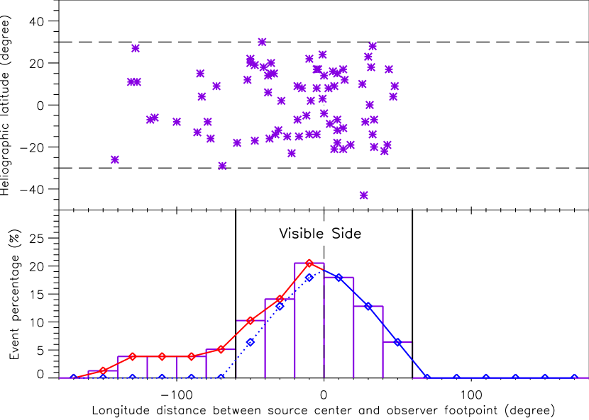
Figure 1: Spatial distribution of the solar sources of 78 solar proton events observed near the Earth’s orbit during 1996-2011. Upper panel: latitudinal and longitudinal distribution. Lower panel: number percentage distribution of the solar events along the relative longitude $\phi_{r}$. Adapted from Figure 1 of He & Wan (2013).

We present the statistical result of the solar proton events in Figure 1. A preliminary result was reported in He & Wan (2013). In the upper panel, it can be seen that the solar flares are primarily distributed within $[S30^{\circ},N30^{\circ}]$, which is consistent with the result in Zhao et al. (2007). We divide the relative longitude $\phi_{r}$ into bins: $[-180^{\circ},-160^{\circ}]$, $[-160^{\circ},-140^{\circ}]$, $\ldots$, $[160^{\circ},180^{\circ}]$. The number percentage distribution of the solar events along the relative longitude $\phi_{r}$ is presented in the lower panel. We note that the negative value (left) and positive value (right) indicate that the solar flares locate on the eastern side and western side of the magnetic footpoint of observer, respectively. To directly compare the event number percentages between the east and west relative longitude, the event number percentages on the right side are mirrored to the left side, indicated by a blue dotted line. We mainly pay attention to the central longitude range of the visible side of the Sun, as indicated between the two vertical lines in Figure 1. It can be seen that with the same longitudinal separation between the magnetic footpoint of observer and solar sources, the number of the solar proton events originating from sources located on the eastern side of the observer’s magnetic footpoint is larger than the number of the solar proton events from sources located on the western side (He & Wan, 2013).

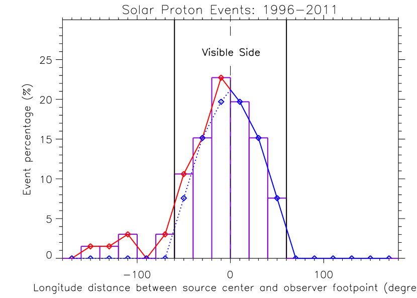
Figure 2: Number percentage distribution of the solar sources of the 66 SEP events with relatively short delays along the relative longitude $\phi_{r}$. With the same longitudinal distance between the observer’s magnetic footpoint and solar sources, the number of the SEP events originating from sources located on the eastern (left) side of the observer’s footpoint is larger than the number of the SEP events from sources located on the western (right) side.

Generally, a SEP event which starts with a long delay at the observer is more possibly related to a CME-driven shock. So we further collect 66 SEP events from Table 1 by excluding the events with a delay of more than 24 hours with respect to the flare maximum. We also statistically investigate the number percentage distribution of these 66 SEP events along the relative longitude $\phi_{r}$. Figure 2 shows the statistical results. We also pay attention to the central longitude range of the visible side of the Sun. As we can see, the number percentage of the SEP events on the left side is generally larger than that on the right side, similar to the results in Figure 1. As noted above, most of the high-energy SEPs (associated with either flares or CME-driven shocks) are probably produced near the Sun. After the SEPs are released on or near the Sun, they will transport in the interplanetary magnetic field with turbulence. During the transport processes in the heliosphere, the parallel diffusion and perpendicular diffusion play a very important role in the SEP distribution and anisotropy. Therefore, we note that even for CME-associated SEP events, the East-West longitudinal (azimuthal) asymmetry of SEP distribution, due to the effects of perpendicular diffusion, will hold. In this sense, it is not very necessary to particularly discriminate between the two types of SEP sources, i.e., solar flares and CME-driven shocks. Actually, the traditional classification paradigm of the so-called impulsive and gradual SEP events is increasingly challenged by the current multi-spacecraft observations (STEREO-A/B, ACE, SOHO, Wind, etc.) and the numerical modeling of three-dimensional focused transport of SEPs.

4 Discussions on the Mechanism Responsible for East-West Azimuthal Asymmetry of SEPs

Our previous numerical simulations of SEP transport with the effect of perpendicular diffusion demonstrated that there exists an East-West longitudinal (azimuthal) asymmetry both in the entire intensities and in the peak intensities of SEPs transporting in the interplanetary space (see He et al., 2011; He & Wan, 2013, 2015). As pointed out by these works, the longitudinally (azimuthally) asymmetric distribution of SEPs results from the East-West azimuthal asymmetry in the geometry of the Parker interplanetary magnetic field as well as the effects of perpendicular diffusion on the transport processes of SEPs in the heliosphere. The formation mechanism of the East-West longitudinal (azimuthal) asymmetry of SEP distribution via perpendicular diffusion is sketched in Figure 3, which is referred to the physical scenario of “multiple SEP events with one spacecraft". The SEP transport in the interplanetary magnetic field mainly includes the parallel diffusion and the perpendicular diffusion. Due to the effect of the perpendicular diffusion, the SEPs released from acceleration regions with limited coverage can cross the interplanetary magnetic field lines and transport to distant heliospheric locations with very wide longitudinal or/and latitudinal separations. In Figure 3, the intensity of SEPs (detected at spacecraft’s position $O_{2}$) originating from solar source A (as an example) located on the eastern side of the observer footpoint is nearly equivalent to the SEP intensity at position $A_{1}$, in a statistical sense. Similarly, the intensity of SEPs (detected at spacecraft’s position $O_{2}$) released from solar source B (with the same longitudinal separation as source A relative to the observer footpoint) located on the western side is nearly equivalent to the SEP intensity at position $B_{1}$, in a statistical sense. As one can see, the heliocentric radial distance $\overline{OA_{1}}$ between solar center (O) and the position $A_{1}$ is shorter than that $\overline{OB_{1}}$ between solar center (O) and the position $B_{1}$. Note that the extent of the length difference between the heliocentric radial distances $\overline{OA_{1}}$ and $\overline{OB_{1}}$ depends on the longitudinal separation between the sources and the observer’s footpoint. Specifically, a larger longitudinal separation leads to a more significant length difference between the radial distances of the east and west equivalent positions (e.g., $A_{1}$ and $B_{1}$ in Figure 3).

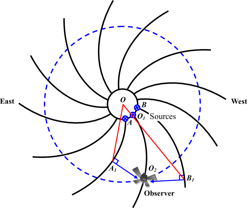
Figure 3: Diagram to illustrate the formation of the East-West longitudinal (azimuthal) asymmetry of SEP distribution via perpendicular diffusion in the physical scenario of “multiple SEP events with one spacecraft". In a statistical sense, the intensity of SEPs (detected at position $O_{2}$) originating from solar source A (B) located on the eastern (western) side of the observer footpoint is nearly equivalent to the SEP intensity at position $A_{1}$ ($B_{1}$). The heliocentric radial distance $\overline{OA_{1}}$ between solar center (O) and the position $A_{1}$ is shorter than that $\overline{OB_{1}}$ between solar center (O) and the position $B_{1}$.

Observational analysis showed that the peak intensities of SEPs decrease with the heliocentric radial distance (r) in a functional form of $r^{-\alpha}$, with $\alpha$ varying in a wide range. Basically, our numerical modeling of the five-dimensional Fokker-Planck transport equation has confirmed these observational results. In this paper, we present a numerical modeling result in Figure 4 regarding radial dependence of intensity-time profiles and peak intensities of SEPs observed along the nominal Parker magnetic field line connecting the spacecraft with the solar source. The upper panel of Figure 4 presents the intensity-time profiles of $32$ MeV protons observed at different heliocentric radial distances: $0.25$, $0.4$, $0.6$, $0.8$, and $1.0$ AU. Both the solar source and the observers are located at $90^{\circ}$ colatitude in this typical case study. As one can see, during the entire evolution process, the particle intensity observed at a smaller radial distance is higher than the particle intensity detected at a larger radial distance.

In addition, we can obviously see that during the late phase, the intensity-time profiles of all the SEP cases display nearly the same decay rate, which is known as the SEP reservoir phenomenon in spacecraft observations (e.g., Roelof et al., 1992). Therefore, our simulations of a series of SEP cases with different radial distances reproduce the so-called SEP reservoir phenomenon. Actually, our numerical simulations with perpendicular diffusion reproduced various SEP reservoirs at different heliospheric locations (longitude, latitude, and radial distance) without invoking the prevailing hypothesis of a reflecting boundary (magnetic mirror) or diffusion barrier (solar wind structure) (e.g., He et al., 2011; He & Wan, 2015; He, 2015). Additionally, so far no any explicit observational evidence or quantitative description of reflecting boundaries (magnetic mirrors) or diffusion barriers (solar wind structures), which were once prevalently supposed to exist in the heliosphere to contain the particles long enough to form the observed SEP reservoirs, has been provided or specified within the community (for discussions, see He, 2015). Actually, as He & Wan (2015) and He (2015) pointed out, it is difficult to imagine such an “overwhelming" reflecting boundary (magnetic mirror) or diffusion barrier (solar wind structure) covering all of the longitudes, all of the latitudes, and even all of the radial distances, and even exactly accompanying almost all of the SEP events including the so-called impulsive or ³He-rich events. Therefore, in the sense of perpendicular diffusion, we suggest that the so-called SEP “reservoir" should be renamed SEP “flood", which is more appropriate to illustrate the transport processes of SEPs in the heliosphere.

In the upper panel of Figure 4, the filled circles with different colors on the intensity-time profiles denote the peak intensities of the corresponding SEP cases. We extract the information of the peak intensities and the relevant radial distances in the SEP cases, and present it in the lower panel of Figure 4. We further model the radial dependence of the peak intensities $I_{max}$ with a power-law function $I_{max}(r)=kr^{-\alpha}$, where $k$ is a constant in this case study. We obtain the power-law index $\alpha=1.7$ in this series of SEP cases. We note that the index $\alpha$ mainly depends on the properties (e.g., coverage, location) of SEP sources and the relative locations of magnetic field line footpoints of the observers. From the lower panel of Figure 4, we can clearly see that the peak particle intensities of SEP events exponentially decrease with the increasing radial distances.

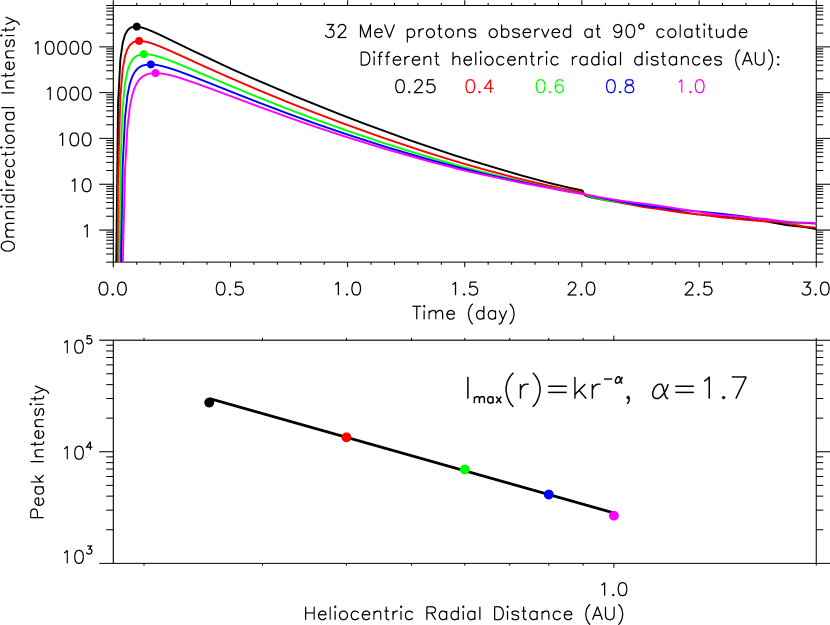
Figure 4: Simulated radial dependence of intensity-time profiles and peak intensities of SEPs observed along the nominal Parker magnetic field line connecting the solar source. Upper panel: The intensity-time profiles of $32$ MeV protons observed at different radial distances: $0.25$, $0.4$, $0.6$, $0.8$, and $1.0$ AU. Both the solar source and the observers are located at $90^{\circ}$ colatitude. Note that the so-called SEP reservoir phenomenon is reproduced in the simulations of a series of SEP cases with different radial distances. Lower panel: The radial dependence of the SEP peak intensities extracted from the intensity-time profiles shown in the upper panel. A functional form of $I_{max}(r)=kr^{-\alpha}$ with index $\alpha=1.7$ is obtained.

According to the relationship $\overline{OA_{1}}<\overline{OB_{1}}$ sketched in Figure 3 and the radial dependence of SEP peak intensities $I_{max}(r)=kr^{-\alpha}$ with, e.g., $\alpha=1.7$ in this work, we can readily deduce that the peak intensity observed at position $A_{1}$ is larger than that observed at position $B_{1}$. Actually as shown in the upper panel of Figure 4, the SEP intensity detected at position $A_{1}$ is larger than that detected at position $B_{1}$ through the whole evolution process. We also note that these results are valid for arbitrary energies of energetic particles and for arbitrary particle species including electrons and heavy ions. Therefore, the particle fluence and radiation dose received at position $A_{1}$ are, respectively, higher than those received at position $B_{1}$. Then according to the intensity equivalence relationship discussed above between $A_{1}$ and $O_{2}$ (observing SEPs from source A) as well as that between $B_{1}$ and $O_{2}$ (observing SEPs from source B), we can infer that the entire intensity, peak intensity, particle fluence, and radiation dose originating from source A are, respectively, larger than those originating from source B. We note that these conclusions hold for arbitrary couple of solar sources located on the eastern and western sides of the observer’s magnetic footpoint, respectively, but with the same longitudinal separation relative to the observer’s magnetic footpoint.

In typical cases of interplanetary conditions, the perpendicular diffusion coefficient should be smaller than the parallel diffusion coefficient, as performed in our previous numerical modeling, although the effect of perpendicular diffusion always plays a very important role in the transport and distribution of SEPs. Therefore, we note that the longitudinal separation between the source region and the magnetic footpoint of the observer is the most crucial factor in determining the longitudinal variation of the entire intensity and the peak intensity of SEPs, indicating that the farther the magnetic footpoint of the observer is away from the solar source, the smaller the SEP intensity will be observed by the spacecraft and also the later the SEP event onset will be detected.

The probability of an SEP event being detected by spacecraft in the interplanetary space is related to the SEP intensity in the event and the detection threshold of the instruments onboard the spacecraft. In addition, note that the criterion of an event being recorded in the SPE listing of NOAA is that the flux of the event being larger than or equal to 10 pfu. Therefore, the spacecraft detection threshold and SPE listing criterion naturally play a role in the historical records of SEP events affecting the Earth environment. Our previous simulations showed that with the same longitudinal separations between the solar sources and the magnetic footpoint of the observer, the SEP events originating from solar sources on the eastern side of the magnetic footpoint of the observer reveal larger fluxes than those from solar sources on the western side (He et al., 2011; He & Wan, 2015). Therefore, the SEP events from solar sources on the eastern (western) side of observer’s magnetic footpoint will have a larger (smaller) probability of being detected and recorded by spacecraft near the Earth’s orbit. When a large data set of SEP events is taken into account, it is natural and expectable to obtain the East-West longitudinal (azimuthal) asymmetry (Figures 1 and 2). As discussed above, the detection threshold and listing criterion naturally play a role in the statistical results of the East-West longitudinally (azimuthally) asymmetric distribution of SEP events. We point out that no matter what the detection threshold (e.g., particle flux, particle energy, particle species, etc.) or listing criterion is, the result of the East-West longitudinal (azimuthal) asymmetry of SEP events will hold, provided that a relatively large data set is taken into account. We emphasize that our numerical simulations of five-dimensional transport equation and statistical analysis of SEP events confirm each other. Furthermore, the combination of statistical survey and numerical modeling regarding the East-West longitudinal (azimuthal) asymmetry presents a unique evidence for the effects of perpendicular diffusion on the SEP propagation in the heliosphere.

5 Relationship between Our Results and Those of a Recent Work

In a recent work (Dresing et al., 2014), the authors also presented a statistical survey of the longitudinal distribution of SEP peak intensities observed by twin spacecraft STEREO-A/B and near-Earth spacecraft ACE. A similar investigation of SEP peak intensities can be found in Lario et al. (2013), where the SEP intensity asymmetry was also presented. Essentially, their results, obtained in a “one SEP event with multiple spacecraft" style, are consistent with and confirm our numerical modeling and observational results. In this section, we discuss the relationship between our results and those of Dresing et al. (2014).

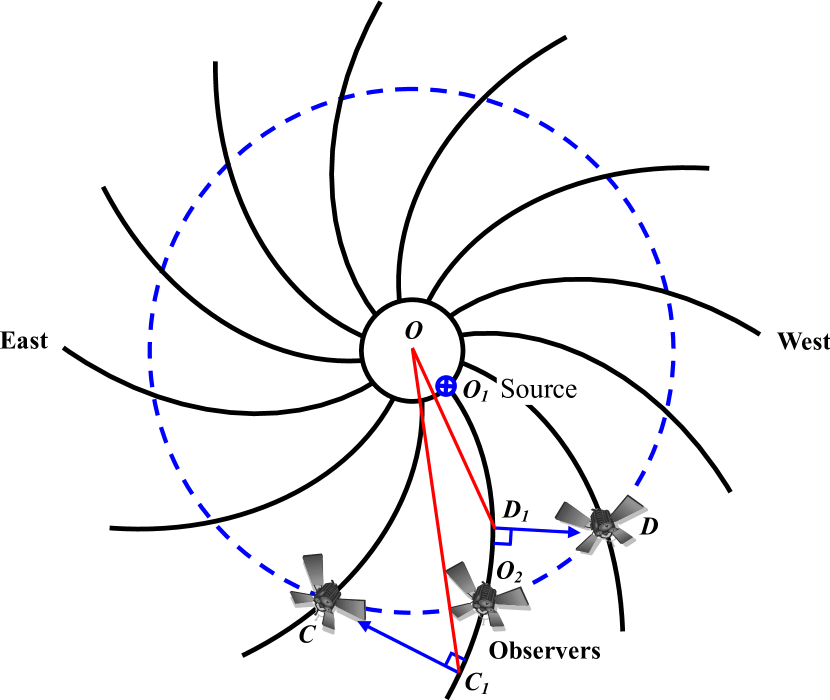
Figure 5: Diagram to illustrate the formation of the East-West longitudinal (azimuthal) asymmetry of SEP distribution via perpendicular diffusion in the physical scenario of “one SEP event with multiple spacecraft". In a statistical sense, the SEP intensity observed by spacecraft D (C) located on the western (eastern) side is nearly equivalent to the SEP intensity observed at position $D_{1}$ ($C_{1}$). The heliocentric radial distance $\overline{OD_{1}}$ between solar center (O) and the position $D_{1}$ is smaller than that $\overline{OC_{1}}$ between solar center (O) and the position $C_{1}$.

Figure 5 sketches the physical scenario of the multi-spacecraft observations of SEPs originating from a common particle source (e.g., source $O_{1}$) on the solar surface. The three spacecraft (marked with C, $O_{2}$, and D, respectively, from East to West) are located at heliospheric positions with the same heliocentric radial distance but with different heliolongitudes. Specifically, the spacecraft $O_{2}$ in the middle is directly connected to the solar source $O_{1}$ by the interplanetary magnetic field line, whereas the magnetic footpoints of the spacecraft C on the left and spacecraft D on the right are located on the eastern side and western side, respectively, with the same longitudinal separation, relative to the solar source $O_{1}$. After being released from the solar surface, the energetic particles will transport diffusively in turbulent interplanetary magnetic field, consisting of parallel diffusion along and perpendicular diffusion across the mean magnetic field. Due to the effects of perpendicular diffusion, the energetic particles released from a solar source (e.g., source $O_{1}$) with limited coverage can be detected by multiple spacecraft with wide longitudinal or/and latitudinal separations between every couple of them. The SEP intensity observed by spacecraft D located on the western side is nearly equivalent to the SEP intensity observed at position $D_{1}$, in a statistical sense. Likewise, the SEP intensity detected by spacecraft C located on the eastern side is nearly equivalent to the SEP intensity detected at position $C_{1}$, in a statistical sense. As we can see, the heliocentric radial distance $\overline{OD_{1}}$ between solar center (O) and the position $D_{1}$ is smaller than that $\overline{OC_{1}}$ between solar center (O) and the position $C_{1}$. Note that the extent of the length difference between the radial distances $\overline{OC_{1}}$ and $\overline{OD_{1}}$ depends on the longitudinal separation between the source and the observer footpoints. A larger longitudinal separation leads to a more considerable length difference between the radial distances $\overline{OC_{1}}$ and $\overline{OD_{1}}$. In combination with the numerical simulation result of the radial dependence of SEP intensity-time profiles and SEP peak intensities ($I_{max}(r)=kr^{-\alpha}$) as shown in Figure 4 and discussed above, we can readily infer that the SEP intensity (both entire intensity and peak intensity) observed at position $D_{1}$ is larger than that observed at position $C_{1}$. According to the intensity equivalence relationship between positions D and $D_{1}$ as well as that between positions C and $C_{1}$, we can infer that the SEP intensity (both entire intensity and peak intensity) observed by the western spacecraft D is larger than that observed by the eastern spacecraft C. As a natural result of interplay between perpendicular diffusion and parallel diffusion, the observation location of the highest intensity-time profile and the largest peak intensity of SEPs will shift from the place of best magnetic connection and slightly toward the west of the associated SEP source. We note that these results are valid for arbitrary energies of energetic particles and for arbitrary particle species including electrons and heavy ions.

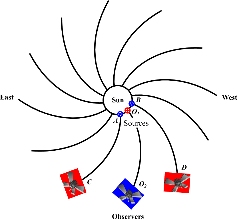
Figure 6: Diagram to illustrate the relationship between the two physical scenarios of “multiple SEP events with one spacecraft" (sources A and B and spacecraft $O_{2}$ labeled in blue) and “one SEP event with multiple spacecraft" (source $O_{1}$ and spacecraft C and D labeled in red). The relative position between source A (B) and spacecraft $O_{2}$ is equivalent to the relative position between source $O_{1}$ and spacecraft D (C). With this “spiral transformation trick", the two physical scenarios are unified and identified with each other.

Figure 6 presents the relationship between our physical scenario and that of Dresing et al. (2014). The SEP sources A and B and spacecraft $O_{2}$ labeled in blue indicate the “multiple SEP events with one spacecraft" scenario, and the SEP source $O_{1}$ and spacecraft C and D labeled in red indicate the “one SEP event with multiple spacecraft" scenario. We emphasize the importance of the concept of “relative position" in understanding the physical relationship between our results and those of Dresing et al. (2014). As shown in Figure 6, the relative position between SEP source A and spacecraft $O_{2}$ is equivalent to the relative position between source $O_{1}$ and spacecraft D; the relative position between source B and spacecraft $O_{2}$ is equivalent to the relative position between source $O_{1}$ and spacecraft C. Therefore, the intensity observed by spacecraft $O_{2}$ of SEPs originating from source A is equivalent to the intensity observed by spacecraft D of SEPs originating from source $O_{1}$; the intensity observed by spacecraft $O_{2}$ of SEPs originating from source B is equivalent to the intensity observed by spacecraft C of SEPs originating from source $O_{1}$. Accordingly, with the same longitudinal separation between the solar source and the magnetic footpoint of the observer, the following two results are essentially the same: (1) in the scenario of “multiple SEP events with one spacecraft", the SEP intensity originating from the solar source (e.g., source A in Figure 6) located at the eastern side of observer footpoint is larger than the SEP intensity originating from the source (e.g., source B) located at the western side; (2) in the scenario of “one SEP event with multiple spacecraft", the SEP intensity observed by the spacecraft (e.g., spacecraft D) located at the western side of the SEP source is larger than the SEP intensity detected by the spacecraft (e.g., spacecraft C) located at the eastern side. By performing such “spiral transformation trick" as shown in Figure 6, the two physical scenarios presented in our works (He et al., 2011; He & Wan, 2013, 2015) and in Dresing et al. (2014) are essentially unified and identified with each other.

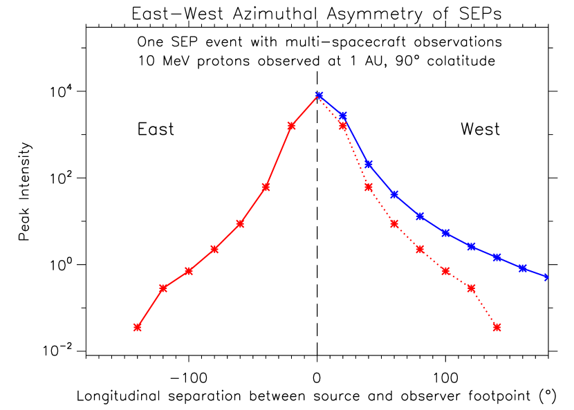
Figure 7: Multidimensional numerical modeling of the East-West longitudinal (azimuthal) asymmetry of SEP distribution in the scenario of “one SEP event with multiple spacecraft". The red (blue) solid line on the left (right) indicates the peak intensities of $10$ MeV protons observed by spacecraft located at the eastern (western) side of the solar source. The red dotted line on the right is mirrored from the left. It can be clearly seen that the SEP peak intensities observed by spacecraft located at the western side of the SEP source are systematically larger than those observed by spacecraft located at the eastern side. In addition, the location of the largest SEP peak intensity slightly shifts to the west of the SEP source.

As an example, Figure 7 presents the multidimensional numerical modeling result of the East-West longitudinal (azimuthal) asymmetry of SEPs in the scenario of “one SEP event with multiple spacecraft". For more details on the numerical model and numerical method of the five-dimensional Fokker-Planck focused transport equation, we refer the reader to our simulation works (e.g., He et al., 2011; He & Wan, 2015; He, 2015). In this work, we only present Figure 7 to demonstrate the relationship between our results and those of Dresing et al. (2014). The red solid line on the left-hand half in Figure 7 indicates the peak intensities of $10$ MeV protons observed by a series of spacecraft located at the eastern side of the nominal magnetic field line connecting the solar source. On the right-hand half of Figure 7, the blue solid line indicates the peak intensities of $10$ MeV protons detected by a series of spacecraft located at the western side of the nominal field line connecting the SEP source. For direct comparison between the two halves, we further mirror the SEP peak intensities from the left-hand half to the right-hand half with a red dotted line. After this operation, we can clearly see that the SEP peak intensities observed by spacecraft located at the western side of the SEP source are systematically larger than those observed by spacecraft located at the eastern side. According to the discussions above and our numerical simulations, actually, during the entire evolution process, the SEP intensity observed at the western side is larger than that observed at the eastern side, provided that the magnetic footpoints of the pair of observers located at the western and eastern sides, respectively, are with the same longitudinal separation relative to the SEP source. In addition, due to the interplay between perpendicular diffusion and parallel diffusion, the longitudinal location at which the largest SEP peak intensity is observed slightly shifts to somewhere on the western side of the SEP source. Basically, the accurate extent of west-shift depends on the ratio of perpendicular to parallel diffusion coefficients, geometry of the Parker magnetic spiral (corresponding to solar wind speed), particle energy and species, coverage of the SEP sources, and particle spatial distribution in the sources.

6 Summary and Conclusions

He et al. (2011) reported that with the same longitudinal separation between magnetic footpoint of observer and SEP sources, the SEPs produced from the sources located east are detected earlier with higher fluxes than those associated with the sources located west (see also He & Wan, 2013, 2015). Our statistical survey of solar proton events showed that with the same longitudinal separation between the observer’s magnetic footpoint and the SEP sources, the number of SEP events associated with the sources located on the eastern side of the observer’s magnetic footpoint is larger than the number of the SEP events originating from the sources located on the western side. Generally, the probability of a solar proton event being observed by spacecraft in the interplanetary space depends on the SEP intensity in the event as well as the instrumental sensitivity threshold of the spacecraft. Therefore, our statistical analysis of SEP events accumulated over 16 years and our numerical simulations of the five-dimensional Fokker-Planck transport equation modeling taking into account perpendicular diffusion confirm each other. We further point out that the statistical results of solar proton events accumulated over a long time period provide an observational evidence for the effects of perpendicular diffusion on the SEP propagation in the interplanetary space.

We discuss in detail the effects of perpendicular diffusion on the formation of the East-West longitudinally (azimuthally) asymmetric distribution of SEPs. The role of perpendicular diffusion in the physical scenarios of both “multiple SEP events with one spacecraft" and “one SEP event with multiple spacecraft" is thoroughly demonstrated. We obtain the radial dependence of SEP peak intensities $I_{max}(r)=kr^{-1.7}$ from numerically modeling the five-dimensional Fokker-Planck focused transport equation. We employ this functional relation ($I_{max}(r)=kr^{-1.7}$) to quantitatively illustrate and explain the East-West longitudinal (azimuthal) asymmetry of SEP distribution in the heliosphere. The inherent relationship between our results (He et al., 2011; He & Wan, 2013, 2015) and those of Dresing et al. (2014) is comprehensively discussed. In the context of perpendicular diffusion, our results and those of Dresing et al. (2014) are essentially unified and identified with each other. We note that the SEP phenomenon of longitudinally (azimuthally) asymmetric distribution (“East-West azimuthal asymmetry") cannot be decently explained by any other hypothetical mechanisms including the so-called reflecting boundary (magnetic mirror) and diffusion barrier (solar wind structure).

In this work, we primarily discuss the SEP scenario in the ecliptic plane. It should be noted that the results and the conclusions presented above essentially hold for arbitrary heliospheric latitudes. As a special and unique SEP phenomenon, the East-West longitudinally (azimuthally) asymmetric distribution of SEPs represents the important effects of the perpendicular diffusion processes (which was usually ignored in previous studies, especially in the observational community) and of the large-scale Parker spiral geometry of the interplanetary magnetic field. In addition, we note that the East-West longitudinal (azimuthal) asymmetry of SEP distribution is a universal phenomenon independent of particle energy, particle species, particle origin (on or near the Sun or in the interplanetary space), and observer’s location (latitude, longitude, and radial distance) in the heliosphere. Therefore, our results presented in this work will be valuable for understanding the Sun-Earth relations and especially for understanding the three-dimensional propagation of SEPs in the heliosphere.

Appendix A List of Solar Proton Events

We list here the solar proton events analyzed in this study. See Table 1 for details.

Table 1: Solar Proton Events Affecting the Earth Environment (1996-2011)(collected from Space Weather Prediction Center of NOAA)

Solar Proton Event Associated CME Flare and Active Region Solar Wind Speed Start Maximum Proton Flux Onset Flare Maximum Importance Location Region No. SOHO ACE Mean (Day/UT) (Day/UT) (pfu @ $>10$ MeV) (Direction/Day/UT) (Day/UT) (X Ray/Opt.) $(km~{}s^{-1})$ 1997.11.04/08:30 1997.11.04/11:20 72 W/04/06:10 1997.11.04/05:58 X2/2B S14W33 8100 343 1997.11.06/13:05 1997.11.07/02:55 490 W/06/$>$13:00 1997.11.06/11:55 X9/2B S18W63 8100 425 1998.04.20/14:00 1998.04.21/12:05 1700 W/20/10:07 1998.04.20/10:21 M1/EPL S43W90 8194 377 354 366 1998.05.02/14:20 1998.05.02/16:50 150 Halo/02/14:06 1998.05.02/13:42 X1/3B S15W15 8210 569 557 563 1998.05.06/08:45 1998.05.06/09:45 210 W/06/08:29 1998.05.06/08:09 X2/1N S11W65 8210 437 461 449 1998.08.24/23:55 1998.08.26/10:55 670 NA 1998.08.24/22:12 X1/3B N30E07 8307 651 1998.09.25/00:10 1998.09.25/01:30 44 NA 1998.09.23/07:13 M7/3B N18E09 8340 713 1998.09.30/15:20 1998.10.01/00:25 1200 NA 1998.09.30/13:50 M2/2N N23W81 8340 456 1998.11.14/08:10 1998.11.14/12:40 310 NA 1998.11.14/05:18 C1/BSL N28W90 8375? 407 1999.01.23/11:05 1999.01.23/11:35 14 NA 1999.01.20/20:04 M5 N27E90 588 1999.05.05/18:20 1999.05.05/19:55 14 Halo/03/06:06 1999.05.03/06:02 M4/2N N15E32 8525 448 423 436 1999.06.04/09:25 1999.06.04/10:55 64 NW/04/07:26 1999.06.04/07:03 M3/2B N17W69 8552 416 408 412 2000.02.18/11:30 2000.02.18/12:15 13 W/18/09:54 2000.02.17/20:35 M1/2N S29E07 8872 368 2000.04.04/20:55 2000.04.05/09:30 55 W/04/16:32 2000.04.04/15:41 C9/2F N16W66 8933 394 382 388 2000.06.07/13:35 2000.06.08/09:40 84 Halo/06/15:54 2000.06.06/15:25 X2/3B N20E18 9026 689 704 697 2000.06.10/18:05 2000.06.10/20:45 46 Halo/10/17:08 2000.06.10/17:02 M5/3B N22W38 9026 479 468 474 2000.07.14/10:45 2000.07.15/12:30 24000 Halo/14/10:54 2000.07.14/10:24 X5/3B N22W07 9077 398 2000.07.22/13:20 2000.07.22/14:05 17 NW/22/12:30 2000.07.22/11:34 M3/2N N14W56 9085 412 411 412 2000.09.12/15:55 2000.09.13/03:40 320 Halo/12/13:31 2000.09.12/12:13 M1/2N S17W09 Filament 397 416 407 2000.10.16/11:25 2000.10.16/18:40 15 Halo/16/07:27 2000.10.16/07:28 M2 N04W90 9182? 527 544 536 2000.10.26/00:40 2000.10.26/03:40 15 Halo/25/08:26 2000.10.25/11:25 C4 N00W90 395 390 393 2000.11.24/15:20 2000.11.26/20:30 940 Halo/24/05:30 2000.11.24/05:02 X2/3B N20W05 9236 530 585 558 2001.01.28/20:25 2001.01.29/06:55 49 Halo/28/15:54 2001.01.28/16:00 M1/1N S04W59 9313 392 395 394 2001.03.29/16:35 2001.03.30/06:10 35 Halo/29/10:26 2001.03.29/10:15 X1/1N N14W12 9393 450 2001.04.02/23:40 2001.04.03/07:45 1110 NW/02/ 22:00 2001.04.02/21:51 X20 N18W82 9393 443 480 462 2001.04.10/08:50 2001.04.11/20:55 355 Halo/10/05:30 2001.04.10/05:26 X2/3B S23W09 9415 724 2001.04.15/14:10 2001.04.15/19:20 951 W/15/14:30 2001.04.15/13:50 X14/2B S20W85 9415 409 496 453 2001.04.28/04:30 2001.04.28/05:00 57 Halo/26/12:30 2001.04.26/13:12 M7/2B N17W31 9433 644 619 632 2001.09.15/14:35 2001.09.15/14:55 11 SW/15/11:54 2001.09.15/11:28 M1/1N S21W49 9608 518 586 552 2001.09.24/12:15 2001.09.25/22:35 12900 Halo/24/10:30 2001.09.24/10:38 X2/2B S16E23 9632 418 2001.10.01/11:45 2001.10.02/08:10 2360 SW/01/05:30 2001.10.01/05:15 M9 S22W91 9628 445 483 464 2001.10.19/22:25 2001.10.19/22:35 11 Halo/19/16:50 2001.10.19/16:30 X1/2B N15W29 9661 352 344 348 2001.10.22/19:10 2001.10.22/21:30 24 SE/22/18:26 2001.10.22/17:59 X1/2B S18E16 9672 532 528 530 2001.11.04/17:05 2001.11.06/02:15 31700 Halo/04/16:35 2001.11.04/16:20 X1/3B N06W18 9684 399 413 406 2001.11.19/12:30 2001.11.20/00:10 34 Halo/17/05:30 2001.11.17/05:25 M2/1N S13E42 9704 522 509 516 2001.11.22/23:20 2001.11.24/05:55 18900 Halo/22/23:30 2001.11.22/23:30 M9/2N S15W34 9704 428 467 448 2001.12.26/06:05 2001.12.26/11:15 779 W/26/05:30 2001.12.26/05:40 M7/1B N08W54 9742 392 383 388 2001.12.29/05:10 2001.12.29/08:15 76 E/28/20:06 2001.12.28/20:45 X3 S26E90 9767 433 439 436 2002.02.20/07:30 2002.02.20/07:55 13 W/20/06:30 2002.02.20/06:12 M5/1N N12W72 9825 400 2002.03.17/08:20 2002.03.17/08:50 13 Halo/15/23:06 2002.03.15/23:10 M2/1F S08W03 9866 278

Solar Proton Event Associated CME Flare and Active Region Solar Wind Speed Start Maximum Proton Flux Onset Flare Maximum Importance Location Region No. SOHO ACE Mean (Day/UT) (Day/UT) (pfu @ $>10$ MeV) (Direction/Day/UT) (Day/UT) (X Ray/Opt.) $(km~{}s^{-1})$ 2002.03.20/15:10 2002.03.20/15:25 19 W/18/02:54 2002.03.18/02:31 M1 S09W46  9866 555 2002.04.17/15:30 2002.04.17/15:40 24 Halo/17/08:26 2002.04.17/08:24 M2/2N S14W34 9906 520 2002.04.21/02:25 2002.04.21/23:20 2520 W/21/01:27 2002.04.21/01:51 X1/1F S14W84 9906 454 2002.05.22/17:55 2002.05.23/10:55 820 Halo/22/03:26 2002.05.22/03:54 C5/DSF S19W56 613 2002.07.16/17:50 2002.07.17/16:00 234 Halo/15/20:30 2002.07.15/20:08 X3/3B N19W01 30 476 2002.08.14/09:00 2002.08.14/16:20 26 NW/14/02:06 2002.08.14/02:12 M2/1N N09W54 61 489 2002.08.22/04:40 2002.08.22/09:40 36 SW/22/02:00 2002.08.22/01:57 M5/2B S07W62 69 439 2002.08.24/01:40 2002.08.24/08:35 317 W/24/01:27 2002.08.24/01:12 X3/1F S08W90 69 375 2002.09.07/04:40 2002.09.07/16:50 208 Halo/05/16:54 2002.09.05/17:06 C5/DSF N09E28 102 500 2002.11.09/19:20 2002.11.10/05:40 404 SW/09/13:31 2002.11.09/13:23 M4/2B S12W29 180 376 2003.05.28/23:35 2003.05.29/15:30 121 Halo/28/00:50 2003.05.28/00:27 X3/2B S07W17 365 653 2003.05.31/04:40 2003.05.31/06:45 27 W/31/02:30 2003.05.31/02:24 M9/2B S07W65 365 752 2003.06.18/20:50 2003.06.19/04:50 24 Halo/17/23:30 2003.06.17/22:55 M6 S08E61 386 585 2003.10.26/18:25 2003.10.26/22:35 466 Halo/26/17:54 2003.10.26/18:19 X1/1N N02W38 484 482 2003.10.28/12:15 2003.10.29/06:15 29500 Halo/28/10:54 2003.10.28/11:10 X17/4B S16E08 486 790 2003.11.04/22:25 2003.11.05/06:00 353 Halo/04/1954 2003.11.04/19:29 X28/3B S19W83 486 580 2003.11.21/23:55 2003.11.22/02:30 13 SW/21/00:26 2003.11.20/23:53 M5/2B N02W17 501 494 2004.04.11/11:35 2004.04.11/18:45 35 SW/11/04:30 2004.04.11/04:19 C9/1F S14W47 588 440 2004.07.25/18:55 2004.07.26/22:50 2086 Halo/25/15:30 2004.07.25/15:14 M1/1F N08W33 652 783 2004.09.13/21:05 2004.09.14/00:05 273 Halo/12/00:36 2004.09.12/00:56 M4/2N N04E42 672 554 2004.09.19/19:25 2004.09.20/01:00 57 W/19/22:24 2004.09.19/17:12 M1 N03W58 672 387 2004.11.07/19:10 2004.11.08/01:15 495 Halo/07/17:06 2004.11.07/16:06 X2 N09W17 696 642 2005.01.16/02:10 2005.01.17/17:50 5040 Halo/15/23:06 2005.01.15/23:02 X2 N15W05 720 586 2005.05.14/05:25 2005.05.15/02:40 3140 Halo/13/17:22 2005.05.13/16:57 M8/2B N12E11 759 556 2005.06.16/22:00 2005.06.17/05:00 44 W/16/20:03 2005.06.16/20:22 M4 N09W87 775 592 2005.07.14/02:45 2005.07.15/03:45 134 Halo/13/14:30 2005.07.13/14:49 M5 N10W80 786 430 2005.07.27/23:00 2005.07.29/17:15 41 Halo/27/04:54 2005.07.27/05:02 M3 N11E90 792 554 2005.08.22/20:40 2005.08.23/10:45 330 Halo/22/17:30 2005.08.22/17:27 M5/1N S12W60 798 457 2005.09.08/02:15 2005.09.11/04:25 1880 E/07/17:23 2005.09.07/17:40 X17/3B S06E89 808 873 2006.12.06/15:55 2006.12.07/19:30 1980 Halo 2006.12.05/10:35 X9/2N S07E79 930 580 2006.12.13/03:10 2006.12.13/09:25 698 Halo/13/02:54 2006.12.13/02:40 X3/4B S05W23 930 641 2010.08.14/12:30 2010.08.14/12:45 14 W/14/13:25 2010.08.14/10:05 C4/0F N17W52 1099 409 2011.03.08/01:05 2011.03.08/08:00 50 NW/07/20:00 2011.03.07/20:12 M3/SF N24W59 1164 379 2011.06.07/08:20 2011.06.07/18:20 72 SW/08/17:50 2011.06.07/08:03 M2/2N S21W64 1226 457 2011.08.04/06:35 2011.08.05/21:50 96 NW/06/05:15 2011.08.04/04:12 M9/2B N15W49 1261 583 2011.08.09/08:45 2011.08.09/12:10 26 NW/09/17:10 2011.08.09/08:05 X6/2B N17W83 1263 588 2011.09.23/22:55 2011.09.26/11:55 35 NE/27/04:30 2011.09.22/11:01 X1/2N N11E74 1302 428 2011.11.26/11:25 2011.11.27/01:25 80 NW/28/01:45 2011.11.26/07:10 C1 N08W49 1353 358

References

- Beeck & Wibberenz (1986) Beeck, J., & Wibberenz, G. 1986, ApJ, 311, 437
- Beeck et al. (1987) Beeck, J., Mason, G. M., Hamilton, D. C., et al. 1987, ApJ, 322, 1052
- Cliver & Cane (2002) Cliver, E. W., & Cane, H. V. 2002, EOS Trans. AGU, 83, 61
- Dresing et al. (2014) Dresing, N., Gómez-Herrero, R., Heber, B., et al. 2014, A&A, 567, A27
- Dresing et al. (2012) Dresing, N., Gómez-Herrero, R., Klassen, A., Heber, B., Kartavykh, Y., & Dröge, W. 2012, Sol. Phys., 281, 281
- Dröge et al. (2014) Dröge, W., Kartavykh, Y. Y., Dresing, N., Heber, B., & Klassen, A. 2014, J. Geophys. Res., 119, 6074
- Dröge et al. (2010) Dröge, W., Kartavykh, Y. Y., Klecker, B., & Kovaltsov, G. A. 2010, ApJ, 709, 912
- Effenberger et al. (2012) Effenberger, F., Fichtner, H., Scherer, K., et al. 2012, ApJ, 750, 108
- Giacalone & Jokipii (2012) Giacalone, J., & Jokipii, J. R. 2012, ApJ, 751, L33
- Hasselmann & Wibberenz (1968) Hasselmann, K., & Wibberenz, G. 1968, Z. Geophys., 34, 353
- Hasselmann & Wibberenz (1970) Hasselmann, K., & Wibberenz, G. 1970, ApJ, 162, 1049
- He et al. (2011) He, H.-Q., Qin, G., & Zhang, M. 2011, ApJ, 734, 74
- He & Wan (2013) He, H.-Q., & Wan, W. 2013, Proc. ICRC (Brazil), paper 0267, arXiv:1502.03090
- He & Wan (2015) He, H.-Q., & Wan, W. 2015, ApJS, 218, 17
- He (2015) He, H.-Q. 2015, ApJ, 814, 157
- Jokipii (1966) Jokipii, J. R. 1966, ApJ, 146, 480
- Kelly et al. (2012) Kelly, J., Dalla, S., & Laitinen, T. 2012, ApJ, 750, 47
- Lario et al. (2013) Lario, D., Aran, A., Gómez-Herrero, R., et al. 2013, ApJ, 767, 41
- Parker (1958) Parker, E. N. 1958, ApJ, 128, 664
- Roelof et al. (1992) Roelof, E. C., Gold, R. E., Simnett, G. M., Tappin, S. J., Armstrong, T. P., & Lanzerotti, L. J. 1992, Geophys. Res. Lett., 19, 1243
- Shalchi (2005) Shalchi, A. 2005, MNRAS, 363, 107
- Strauss & Fichtner (2015) Strauss, R. D., & Fichtner, H. 2015, ApJ, 801, 29
- Veselovsky et al. (2004) Veselovsky, I. S., Panasyuk, M. I., Avdyushin, S. I., et al. 2004, Cosmic Research, 42, 435
- Zhang et al. (2009) Zhang, M., Qin, G., & Rassoul, H. 2009, ApJ, 692, 109
- Zhao et al. (2007) Zhao, X., Feng, X., & Wu, C.-C. 2007, J. Geophys. Res., 112, A06107