Model-Free Closed-Loop Stability Analysis:
A Linear Functional Approach

Abstract

Performing a stability analysis during the design of any electronic circuit is critical to guarantee its correct operation. A closed-loop stability analysis can be performed by analysing the impedance presented by the circuit at a well-chosen node without internal access to the simulator. If any of the poles of this impedance lie in the complex right half-plane, the circuit is unstable. The classic way to detect unstable poles is to fit a rational model on the impedance.

In this paper, a projection-based method is proposed which splits the impedance into a stable and an unstable part by projecting on an orthogonal basis of stable and unstable functions. When the unstable part lies significantly above the interpolation error of the method, the circuit is considered unstable. Working with a projection provides one, at small cost, with a first appraisal of the unstable part of the system.

Both small-signal and large-signal stability analysis can be performed with this projection-based method. In the small-signal case, a low-order rational approximation can be fitted on the unstable part to find the location of the unstable poles.

Frequency domain simulation methods, like Harmonic Balance (HB) or a DC analysis, impose a structure on the obtained solution of the circuit [1]: The DC analysis only allows for a fixed solution, while HB imposes a frequency grid. Any circuit solution that requires more than the imposed frequencies, e.g. an extra oscillation not on the imposed grid, cannot be represented in the constrained frequency grids of DC and HB. The simulator will still find a valid solution, but the obtained orbit will be locally unstable: it cannot recover from small perturbations and will be physically unobservable in the circuit [2]. It is therefore necessary to perform a local stability analysis on each of the circuit solutions obtained with a DC and HB analysis [1].

Over the years, several methods have been developed to determine the local stability of a circuit solution. Some techniques, like the analysis of the characteristic system [2], require access to the simulator. Open-loop techniques, like the analysis of the normalised determinant [1], require access to the intrinsic device models. These classic techniques are therefore hard to implement in commercial simulators.

Closed-loop stability analysis methods can easily be applied as a post-processing step without any internal knowledge of the circuit and can be used in commercial simulators. This is the reason why they have attracted a large interest lately [1, 3, 4]. A closed-loop local stability analysis performs linearisation of the circuit around the orbit to check the stability thereof: if the linearised circuit has at least one pole in the complex right half-plane, the orbit is unstable. It is moreover assumed that, conversely, the absence of unstable pole implies stability, although no published proof of this fact seems available yet. The question is more subtle than it looks: there exist delay systems which are unstable and still their transfer-function has no unstable pole [5], moreover has an example of an ideal circuit with this property. Nevertheless, it is claimed in [6] that a circuit whose elements are passive at arbitrary high frequencies must indeed have some unstable pole if it is unstable.

The poles of the linearisation around the circuit orbit cannot be obtained directly. Instead a FRF of the linearised circuit is obtained with small-signal simulations on a discrete set of frequencies. The closed-loop stability analysis then aims at determining whether the underlying FRF has a pole in the complex right half-plane. In a pole-zero stability analysis, a rational approximation is fitted on the FRFs. If the rational approximation contains poles in the complex right half-plane, the solution is declared unstable.

Note that the FRF of circuits with distributed elements, like transmission lines, is not rational. Therefore it must be argued that the poles of the computed rational approximant convey information on the poles of the true FRF. This is a delicate issue and a particular instance of a recurring question in approximation theory, namely: what do the singularities of an approximant tell us about the singularities of the approximated function? We observe that no such information can be drawn from the mere quality of approximation in a range of frequencies, since a famous theorem by Runge entails that a continuous function on a segment can be approximated arbitrary well by a proper rational function with prescribed pole location [7]. Thus, for singularity detection, the choice of the approximation algorithm (and not just the fit of the approximant) does matter.

For instance, methods based on linear interpolation, like Padé or multipoint Padé approximation, are famous for generating spurious poles that wander about the domain of analyticity of the approximated function. This phenomenon was intensively studied for meromorphic and branching functions [8, 9, 10], in particular the convergence in capacity of Padé approximants implies that spurious poles have a nearby zero when the order gets large, leading to so-called near pole-zero cancellations (also known as Froissart doublets). Modifications of Padé approximants were proposed to offset this issue [11], but they do not eliminate the problem [12]. Apparently, the theoretically less studied vector fitting method which is a least squares version of linear interpolation, popular today in system analysis, is also prone to producing spurious poles and near cancellations (see [13] for issues on convergence of this method).

In system identification, near cancellations are often ascribed to overmodelling. The terminology suggests an analogy with the stochastic identification paradigm: though measurements may not correspond to a rational transfer function, the basic assumption is that they arise from a well-defined rational system R with added noise. This point of view leads one to postulate the existence of a “correct order” to identify the Frequency Response Function (FRF), i.e. the degree of R, while using a higher degree results in approximating the noise term with inessential, nearly simplifying rational elements. However, if the transfer function is not rational, requirements to keep the degree small conflict with the need to make the approximation error small as well (not to incur undermodelling), thus calling for a compromise akin to the classical trade-off between bias and variance from parametric stochastic identification [14]. To quote [15]: “it is not always trivial to discriminate between overmodelling quasi-cancellations and physical quasi- cancellations that really reflect an unstable behaviour”.

To resolve this issue, the approach proposed in [15] is to cut the frequency band into smaller intervals and use low-order local rational approximations to assess the stability of the FRF on each interval separately. On small enough intervals, rational approximation can be performed accurately in low degree, and if unstable poles occur their physical character is checked by re-modelling the FRF locally around each of them and verifying that the unstable pole remains present in the new model. This procedure is commercially available in the STAN tool [16, 17] and successful applications on several examples are reported in [18, 19, 20, 21].

Still, justifying the above-described technique presently rests on heuristic arguments, and putting it to work is likely to require some know-how since several parameters need to be adjusted adequately (Appendix A, for example, shows that local models of a stable FRFs can become unstable). This is why the authors feel that it may be interesting to develop an alternative viewpoint, focusing more on estimating the unstable part of the glsFRF.

Below, we propose a closed-loop stability analysis method devoid of local models, in which the FRF is projected onto the orthogonal basis of stable and unstable functions. If a significant part of the FRF is projected onto the unstable basis functions, the circuit solution is unstable. Calculating the projection boils down to computing a Fourier transform once the FRF is mapped from the imaginary axis to the unit circle. Using the Fast Fourier Transform (FFT), this can be done fast and in a numerically robust way.

Functional projection onto a stable and unstable basis is a linear operation, simple to implement, and no optimisation step is required. No model-order or maximum approximation error needs to be specified. The parameters in the projection method are the frequency range on which the FRF is determined and the amount of simulation points. When the amount of simulated points is too low, an interpolation error is present in the result of the method. It is shown that the level of this error can easily be estimated and used to correctly choose the amount of needed simulation points.

Once the unstable part of the FRF has been obtained, it is compared to the level of the interpolation error to determine whether the unstable part is significant or not. This final step can be done visually, or a significance threshold can be chosen by the user, both will require some experience with the method.

A final benefit of the projection-based approach is that it may help exploiting the fact that the unstable part is rational in a small-signal stability analysis [6]. The unstable part can therefore be approximated by a rational function without influence of the distributed elements, which are projected onto the stable part of the FRF.

The following of the paper is structured as follows: First, the simulation set-up used to determine the FRF of the linearised circuit is discussed (Section I). Then, the details of the functional projection are provided (Section II). In Section III, the method is applied to four examples: First, an artificial example is considered. Then, the small-signal stability of two amplifiers is investigated and finally, the method is applied to investigate the large-signal stability of a circuit.

I Determining the frequency responses

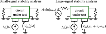
Fig. 1: A Small-signal current source is connected to a well-chosen node in the circuit under test to perform the local stability analysis.

In this paper, the (trans)impedance presented by the circuit to a small-signal current source will be used as FRF (Fig. 1). In the remainder of this paper, it will be assumed that the unstable poles are observable in the FRF. To reduce the chance of missing an instability in the circuit due to a pole-zero cancellation, many different FRFs can be analysed one-by-one. Having a fast method to determine stability of a single FRF is therefore critical to a robust stability analysis.

The FRF of the linearised circuit is obtained by first placing the circuit in the required orbit, using either a DC or HB analysis and running a small-signal simulation around this orbit.

In a small-signal stability analysis, the stability of the DC solution of the circuit is investigated, so the FRF of the linearised circuit is obtained with an AC simulation. The impedance of the circuit is then obtained as:

$$Z_{mn}\!\left(j\omega\right)=\frac{V_{m}\!\left(j\omega\right)}{I_{n}\!\left(j\omega\right)}$$ (1)

where $I_{n}\!\left(j\omega\right)$ is the small-signal current injected into the selected node $n$ and $V_{m}\!\left(j\omega\right)$ is the voltage response of the circuit measured at node $m$ in the circuit.

In a large-signal stability analysis, the stability of a large-signal solution of the circuit is investigated. The circuit is driven by a periodic continuous-wave excitation at a pulsation $\omega_{\mathrm{ex}}$ and the circuit solution is obtained with a HB simulation.

The FRF of the linearised system around the HB orbit is obtained with a mixer-like simulation. As the small-signal will mix with the large signal, several transfer impedances with a different frequency translation are obtained:

$$Z_{mn}^{\left[b\right]}\!\left(j\omega\right)=\frac{V_{m}\!\left(j\omega+bj\omega_{\mathrm{ex}}\right)}{I_{n}\!\left(j\omega\right)}\quad b\in\mathbb{Z}$$

The stability analysis now needs to determine whether the obtained impedances have poles in the right half-plane. The stability analysis of a large-signal orbit doesn’t differ much from the analysis of a DC solution [4]. The small-signal stability analysis can be considered a special case where only $Z_{mn}^{\left[0\right]}\!\left(j\omega\right)$ is analysed.

II Stable/unstable projection

The projection described here has been used before to perform stable interpolation and extrapolation of FRF data [22]. With slight modifications, it can be turned into a full-blown stability analysis. We first start with a brief introduction to the notion of Hardy spaces.

The Hardy space $H^{2}(\mathbb{C}^{+})$, is defined as the set of all functions $g$ defined on $\mathbb{C}^{+}$ such that:

• $\forall z\in\mathbb{C}^{+}$, $g$ is holomorphic at $z$

• $\sup_{x>0}\int_{-\infty}^{+\infty}|g(x+j\omega)|^{2}d\omega<\infty$

A classical result [23, 7] states that every function $g\in H^{2}$ admits a limiting function $G(j\omega)$ defined on the imaginary axis $j\mathbb{R}$. The latter is obtained by taking the limit of $g(z)$ when $z$ tends non tangentially toward $j\omega$. Moreover $\forall z\in\mathbb{C}^{+}$, $g(z)$ is equal to the poisson integral of $G$, that is:

$$g(z=x+jy)=\int_{-\infty}^{+\infty}G(j\omega)\frac{x}{x^{2}+(y-\omega)^{2}}d\omega.$$ (2)

The holomorphic nature of $g$ ensures that it is also the Cauchy integral of its boundary value $G$:

$$g(z=x+jy)=\frac{1}{2\pi}\int_{-\infty}^{+\infty}G(j\omega)\frac{1}{j\omega-z}d\omega.$$ (3)

There is a one to one linear correspondence between the Hardy functions $g$ and its boundary value function $G$. Using this identification, $H^{2}(\mathbb{C}^{+})$ becomes a subspace of the Hilbert space $L^{2}\!\left(j\mathbb{R}\right)$ of square integrable functions on $j\mathbb{R}$. A direct consequence of (2) is that $H^{2}(\mathbb{C}^{+})$ is closed in $L^{2}\!\left(j\mathbb{R}\right)$ and therefore admits an orthogonal complement. An important result [23] asserts that, $\left(H^{2}(\mathbb{C}^{+})\right)^{\perp}=H^{2}(\mathbb{C}^{-})$ where $H^{2}(\mathbb{C}^{-})$ is defined exactly as $H^{2}(\mathbb{C}^{+})$ above by replacing $\mathbb{C}^{+}$ by $\mathbb{C}^{-}$ and taking the supremum over $x<0$. We therefore have that

$$L^{2}\!\left(j\mathbb{R}\right)=H^{2}\!\left(\mathbb{C}^{+}\right)\oplus H^{2}\!\left(\mathbb{C}^{-}\right)$$

This decomposition asserts that any square integrable function on $j\mathbb{R}$ decomposes uniquely as the sum of the traces on the imaginary axis, of an analytic function in the right half-plane and a function analytic in the left half-plane. The projection on $H^{2}\!\left(\mathbb{C}^{+}\right)$ defines the stable part of the function. The projection onto $H^{2}\!\left(\mathbb{C}^{-}\right)$ is the unstable part. As an example, consider $P/Q$ a strictly proper ($\deg(P)<\deg(Q)$) rational function devoid of poles on the imaginary axis. We write its partial fraction expansion as,

$$\frac{P(s)}{Q(s)}=\sum_{i\in I^{+}}\sum_{k=1}^{k_{i}}\frac{a_{i,k}}{(s-\lambda_{i})^{k}}+\sum_{i\in I^{-}}\sum_{k=1}^{k_{i}}\frac{a_{i,k}}{(s-\lambda_{i})^{k}}$$

where the $\lambda_{i}^{\prime}s$ with $i\in I^{-}$ are poles belonging to $\mathbb{C}^{-}$, and the ones with $i\in I^{+}$ belong to $\mathbb{C}^{+}$. The strict properness of $P/Q$ ensures its square integrability on $j\mathbb{R}$. By unicity its stable part obtained after projection on $H^{2}\!\left(\mathbb{C}^{+}\right)$ is found to be,

$$\sum_{i\in I^{-}}\sum_{k=1}^{k_{i}}\frac{a_{i,k}}{(s-\lambda_{i})^{k}},$$

while its unstable part is

$$\sum_{i\in I^{+}}\sum_{k=1}^{k_{i}}\frac{a_{i,k}}{(s-\lambda_{i})^{k}}.$$

In the general case the projection boils down to calculating certain inner products of $Z_{mn}^{\left[b\right]}\!\left(j\omega\right)$ with the basis functions $B_{k}$, which form an orthogonal basis of $L^{2}\!\left(j\mathbb{R}\right)$

$$c_{k}=\left\langle Z_{mn}^{\left[b\right]}\!\left(j\omega\right),B_{k}\right\rangle= \intop_{-\infty}^{\infty}Z_{mn}^{\left[b\right]}\!\left(j\omega\right)\overline{B_{k}\!\left(j\omega\right)}d\omega$$ (4)

$$B_{k}\left(s\right)= -\sqrt{\frac{\alpha}{\pi}}\frac{\left(s-\alpha\right)^{k}}{\left(s+\alpha\right)^{k+1}}\qquad k\in\mathbb{Z}$$ (5)

The overbar $\overline{\bullet}$ indicates the complex conjugate. $\alpha$ is a positive constant used for scaling. All $B_{k}$ with $k\geq 0$ create a basis for the stable part, while the $B_{k}$ with negative $k$ form a basis for $H^{2}\!\left(\mathbb{C}^{-}\right)$. Once the $c_{k}$ coefficients are calculated, the stable and unstable parts are easily recovered by calculating

$$Z_{\mathrm{stable}}\!\left(j\omega\right) =\sum_{k=0}^{\infty}c_{k}B_{k}\!\left(j\omega\right)$$ (6)

$$Z_{\mathrm{unstable}}\!\left(j\omega\right) =\sum_{k=1}^{\infty}c_{-k}B_{-k}\!\left(j\omega\right)$$ (7)

The inner product in (4) runs over all frequencies while the impedance function $Z_{mn}^{\left[b\right]}\!\left(j\omega\right)$ is only known over a frequency range $\mathbf{f}=\left[f_{\mathrm{min}},f_{\mathrm{max}}\right]$. To impose the finite frequency band on the data, the impedance is filtered before the analysis

$$Z_{\mathrm{f}}\!\left(j\omega\right)=Z_{mn}^{\left[b\right]}\!\left(j\omega\right)H\!\left(j\omega\right)$$ (8)

The filter $H\!\left(j\omega\right)$ is a high-order elliptic lowpass filter with its first transmission zero placed at $f_{\mathrm{max}}$ that imposes band limitation. This filter will stabilise poles close to its cutoff frequency, so $f_{\mathrm{max}}$ should be chosen well beyond the maximum frequency at which the circuit can become unstable. $f_{\mathrm{min}}$ should be placed very close to DC. If $f_{\mathrm{min}}$ can’t be close to DC, a bandpass filter should be used for $H\!\left(j\omega\right)$. The filtering ensures that $Z_{\mathrm{f}}\!\left(j\omega\right)\in L^{2}\!\left(j\mathbb{R}\right)$ by suppressing anything outside of the frequency band of interest. The smooth decay to zero of $Z_{\mathrm{f}}\!\left(j\omega\right)$ at the edges of the frequency interval will avoid instabilities to pop up due to the discontinuity of $Z_{mn}^{\left[b\right]}\!\left(j\omega\right)$.

In this paper, we use an elliptic filter of order 10 to filter the data. The filter has one transmission zero which is placed exactly at $f_{\mathrm{max}}$.

II-A Transforming to the unit circle

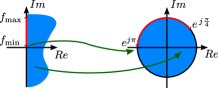
Fig. 2: The Möbius transform used in the analysis maps the complex right-half plane to the inside of the unit disc. DC is mapped to $-1$. When $\alpha=2\pi f_{\mathrm{max}}\left(\sqrt{2}-1\right)$, $f_{\mathrm{max}}$ is mapped to $e^{j\frac{\pi}{4}}$.

Working with the basis functions defined in (5) is troublesome from a numeric point of view. Performing the projection when working on unit disc yields better results [22]. The mapping from the complex plane to the unit circle is performed with the Möbius mapping visualised in Fig. 2:

$$Z_{\mathrm{f}}\!\left(s\right)\underset{\mathrm{M\ddot{o}b}}{\longmapsto}Z_{\mathrm{f}}^{\mathrm{disc}}=\sqrt{\pi\alpha}\frac{2}{z-1}Z_{\mathrm{f}}\left(\alpha\frac{1+z}{1-z}\right)$$ (9)

Our mapping of choice converts square integrable functions on the frequency axis into square integrable functions of the same norm on the unit circle. Square integrable functions which are analytic on the right half-plane are mapped onto square integrable functions which are analytic inside the unit disc. Appendix B shows that the basis functions $B_{k}$ map onto powers of $z$

$$B_{k}\!\left(s\right)\underset{\mathrm{M\ddot{o}b}}{\longmapsto}B_{k}^{\mathrm{disc}}\!\left(z\right)=z^{k}$$ (10)

Projecting on this basis boils down to calculating the Fourier series of $Z_{\mathrm{f}}^{\mathrm{disc}}\!\left(z\right)$, with coefficients given by

$$c_{k}=\frac{1}{2\pi}\intop_{0}^{2\pi}Z_{\mathrm{f}}^{\mathrm{disc}}\left(e^{j\theta}\right)e^{-jk\theta}d\theta$$ (11)

This Fourier series can be calculated in a numerically efficient way using the Fast Fourier Transform (FFT). The FFT requires that the $\theta$-values are linearly spaced between $0$ and $2\pi$. Due to the mapping from the complex plane to the unit disc, the samples will not satisfy this constraint. A simple interpolation, can be used to obtain $Z_{\mathrm{f}}^{\mathrm{disc}}$ on the $\theta$-values required to perform the FFT.

The interpolation can introduce artefacts in the unstable part if the FRF is not sampled on a sufficiently dense frequency grid, which will be shown on an example later. The level of this interpolation error can be estimated by interpolating the FRF using only the data at the even data points. The difference between the original and the interpolated data for the odd data points will give an indication of the interpolation error encountered in the stability analysis. When the unstable part lies significantly above the interpolation error, we can conclude that the original impedance is unstable.

The threshold to determine when the unstable part lies significantly above the level of the interpolation error will depend on the simulation set-up for the circuit. In the examples that follow, a level of $20\leavevmode\nobreak\ \mathrm{dB}$ has been used as a threshold. A more strict threshold could be used at the cost of requiring a more dense frequency grid and an increased simulation time. When measured components are used in the simulation set-up, the noise level in those measurements should be taken into account to choose the correct threshold.

II-B Summary of the projection method

The stable and unstable parts of a FRF are determined using the following steps:

1. Multiply the FRF with a high-order filter as in (8)

2. Transform the filtered FRF to the unit disc using (9)

3. Interpolate the transformed FRF to a linear grid and use the FFT to calculate the $c_{k}$ coefficients

4. Reconstruct the stable and unstable part using (6-7)

II-C Obtaining the unstable poles

A function is meromorphic on $\mathbb{C}$ if it is holomorphic on $\mathbb{C}$ but on a countable number of isolated poles. The function $\tanh(\omega)$ is for example meromorphic, having infinitely many isolated poles on the imaginary axis placed at $j\pi/2+jk\pi\,\,(\forall k\in\mathbb{Z})$ and being analytic elsewhere. In a small-signal stability analysis of a circuit composed of lumped elements, transmission lines and active devices modelled by negative resistors, the impedances can be shown to be meromorphic functions of the frequency. Under the additional realistic assumption that active elements can only deliver power over a finite bandwidth, the impedances are proven to possess only finitely many unstable poles in $\mathbb{C}^{+}$ [6]. Under the generic condition that $Z_{mn}^{\left[b\right]}\!\left(j\omega\right)$ is devoid of poles on the imaginary axis, and that the filtering function $H\!\left(j\omega\right)$ decays strongly enough in order to render $Z_{mn}^{\left[b\right]}\!\left(j\omega\right)H\!\left(j\omega\right)$ square integrable, we conclude that the unstable part of $Z_{mn}^{\left[b\right]}\!\left(j\omega\right)H\!\left(j\omega\right)$ is a rational function. Its poles coincide with the unstable poles of $Z_{mn}^{\left[b\right]}\!\left(j\omega\right)$: note here that the multiplication by $H\!\left(j\omega\right)$ does not add any unstable pole as $H\!\left(j\omega\right)$ is stable. This means that most of the complexity of the frequency response, like the delay, will be projected onto the stable part, while the unstable part can easily be approximated by a low-order rational model to recover the unstable poles.

Classic rational approximation tools can be used to approximate the unstable part and determine the unstable poles. When multiple frequency responses are analysed simultaneously, an approximation method suited for approximation of rational matrices is preferred [24]. In our current implementation, Kung’s method [25, 26] is used to estimate the poles of the unstable part of a single FRF at a time. Alternatively, more sophisticated rational approximation engines like RARL2 [24] can be used to recover and track unstable poles.

Compared to working with a high-order rational approximation of the total impedance of the circuit, the ‘split-first, approximate later’ approach proposed here could be a faster and easier method to recover the unstable poles. The post-processing will be faster, but the amount of points required to obtain a sufficiently low interpolation error might be higher than the amount of points required for a tool based on rational approximation.

When the circuit is stable, designers often require information about critical stable poles, to determine how far the circuit is from instability and to track the location of the poles as the circuit varies. In its current form, the projection-based analysis does not simplify finding the location of the stable poles. To perform such an analysis, methods based on local modelling may still be required.

III Examples

The stability analysis will now be applied to four different examples. The first is an artificial example generated in Matlab on which we can demonstrate that the unstable poles in the circuit are recovered perfectly. In the second example, an unstable balanced amplifier is analysed to show that the method works for RF circuits. The third example is a two-stage GaN Power Amplifier (PA). In the final example, a large-signal stability analysis is performed to verify the stability of a circuit orbit obtained in a HB simulation.

All simulations were performed in Keysight’s Advanced Design System (ADS) and the post-processing was performed in Matlab.

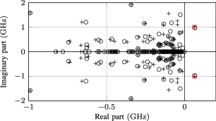
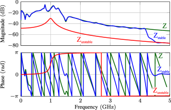
Fig. 3: Pole-zero map of the test system. There are 202 poles ( ) and 200 zeroes ( ). The two poles placed in the right half-plane are easily recovered after the projection by fitting a low-order model on the unstable part ( ).

Fig. 4: The stable/unstable projection splits the original frequency response ( ) in a stable part indicated with ( ) and an unstable part indicated with ( )

III-A Example 1: Random state space system

As a first example, the stability analysis is applied to a random system of order $202$ generated with the rss function from Matlab. The test system has an unstable pole pair at $1\leavevmode\nobreak\ \mathrm{GHz}$, as can be seen on its pole-zero map (Fig. 4). A zero is placed close to the unstable poles. This makes that the unstable poles are difficult to observe in the FRF. To introduce delay in the test system, a time delay of $2\leavevmode\nobreak\ \mathrm{ns}$ is added to the system. The frequency response of the system is calculated on 5000 linearly spaced frequency points between $0\leavevmode\nobreak\ \mathrm{Hz}$ and $5\leavevmode\nobreak\ \mathrm{GHz}$ and is shown in green in Fig. 4. The obtained stable and unstable parts after projection are shown in red and blue on the same figure. The maximum interpolation error is very low in this example ($-120\leavevmode\nobreak\ \mathrm{dB}$) . We will focus on the effect of the interpolation error in more detail in example 2.

The obtained unstable part peaks at $1\leavevmode\nobreak\ \mathrm{GHz}$, which matches the location of the unstable pole pair of the system. Note also that the obtained $Z_{\mathrm{unstable}}$ is very simple: it is clearly a second-order system. Most of the complexity of the frequency response, including the delay, is projected onto the stable part. This observation supports the proposed approach of estimating a rational model only after projection. A good fit was obtained with a rational model that consisted of two unstable poles and a single zero. The two poles obtained with a rational approximation of $Z_{\mathrm{unstable}}$ coincide exactly with the unstable poles in the circuit as is shown in Fig. 4.

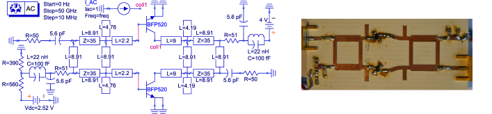
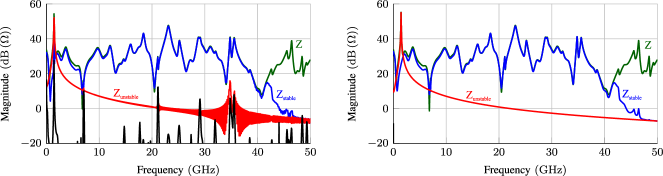
Fig. 5: Simulation set-up and photograph of the balanced amplifier. In the simulations for the stability analysis, the amplifier is excited at the collector of one of its transistors. All transmission lines in the circuit are $50\Omega$ lines unless stated otherwise. The length of the transmission lines is given in millimetres. The TLINP model was used for the transmission lines with $\epsilon_{r}=6.15$, $\tan(\delta)=0.003$ and conductor losses $A=2.5\leavevmode\nobreak\ \nicefrac{{\mathrm{dB}}}{{\mathrm{m}}}$.

Fig. 6: The separation of the impedance ( ) into the stable part ( ) and unstable part ( ) reveals the instability around $1.46\leavevmode\nobreak\ \mathrm{GHz}$. The interpolation error is shown with ( ). In the plot on the left, there are artefacts present in the unstable part due to interpolation of the coarsely obtained impedance data. When the impedance of the balanced amplifier is simulated on a finer frequency grid, the artefacts disappear (right).

III-B Example 2: Balanced amplifier

The second example is a balanced amplifier built as a student project for operation around $3.4\leavevmode\nobreak\ \mathrm{GHz}$ (Fig. 6). Two BFP520 transistors were used to construct the amplifier. During measurement, the design oscillated around $1.43\leavevmode\nobreak\ \mathrm{GHz}$ when terminated with $50\leavevmode\nobreak\ \mathrm{\Omega}$, so the circuit is a good candidate to verify the proposed method to find the instability in simulations.

The small-signal current source was connected to the collector of the top transistor. The BFP520 has a $f_{\mathrm{T}}$ of $45\leavevmode\nobreak\ \mathrm{GHz}$, so the maximum frequency for the simulation was set to $50\leavevmode\nobreak\ \mathrm{GHz}$. The impedance of the circuit was determined starting from DC in $10\leavevmode\nobreak\ \mathrm{MHz}$ steps. The obtained impedance is shown in green in Fig. 6, the obtained stable and unstable parts are also shown in the same figure. The instability around $1.46\leavevmode\nobreak\ \mathrm{GHz}$ is detected, but also some artefacts can be observed in the obtained unstable part at higher frequencies. The high level of the interpolation error at the frequency of these artefacts indicates that they are due to the interpolation in step 3 of the stable/unstable projection. At the frequency of the detected instability, the unstable part lies about $30\leavevmode\nobreak\ \mathrm{dB}$ above the error level, which indicates that the instability is not an interpolation artefact.

To confirm that the artefacts are caused by the interpolation, a second simulation was run, but now $1\leavevmode\nobreak\ \mathrm{MHz}$ steps were used instead of $10\leavevmode\nobreak\ \mathrm{MHz}$. The stable/unstable projection of the denser frequency response data (Fig. 6) still predicts the instability around $1.46\leavevmode\nobreak\ \mathrm{GHz}$, but the artefacts in the unstable part at higher frequencies are gone. The maximum of the interpolation error went down to $-80\leavevmode\nobreak\ \mathrm{dB(\Omega)}$.

III-C Example 3: Two-stage Power Amplifier

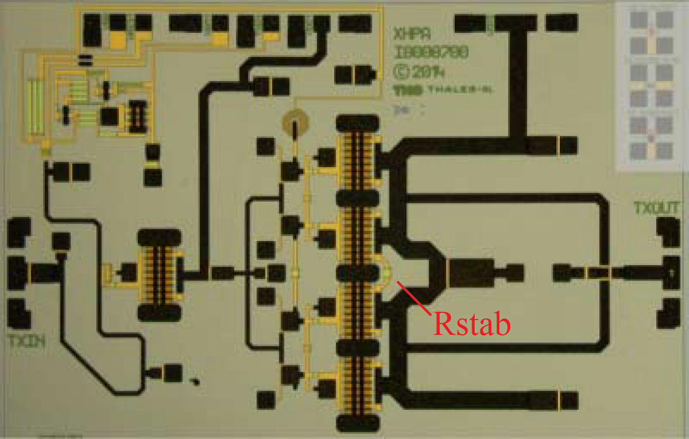
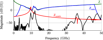
Fig. 7: Microphotograph of the MMIC. The stabilisation resistor $R_{\mathrm{stab}}$ is indicated in red.

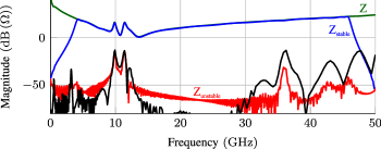
Fig. 8: Impedance seen at the gate of the first stage of the PA for $R_{\mathrm{stab}}=500\Omega$. Its obtained stable and unstable parts clearly indicate that the DC solution of the amplifier is unstable. The interpolation error ( ) is quite high due to the low amount of simulation points.

Fig. 9: Impedance presented by the PA at the gate of the transistor in the first stage for $R_{\mathrm{stab}}=25\Omega$. The obtained stable and unstable parts indicate that the DC solution is now stable. The interpolation error is shown with ( ).

As a third example, we consider the small-signal stability analysis of an X-band PA designed in the $0.25\mathrm{\mu m}$ GaN HEMT technology GH25-10 of UMS [27]. The circuit and its design are described in great detail in [18]. The resulting MMIC is shown in Fig. 9.

The PA is a two-stage design where the second stage consists of two branches with each two transistors in parallel. In simulation, the second stage of the PA demonstrated an odd-mode instability [18], so a stabilisation resistor was added between the drains of the top and bottom halves of the second stage of the PA (as indicated in the Fig.).

The simulation of the complete PA was performed in ADS. The passive structures in the circuit were simulated with EM simulations in Momentum and combined with the non-linear transistor models afterwards. To verify the stability of the amplifier, the circuit impedance was determined at the gate of the top most transistor of the second stage.

The obtained impedance for $R_{\mathrm{stab}}=500\Omega$ is shown in Fig. 9. The impedance is simulated on 945 logarithmically spaced points between $1\mathrm{MHz}$ and $50\mathrm{GHz}$. Because $1\mathrm{MHz}$ is not sufficiently close to DC, a bandpass filter was used in the stability analysis. Due to the low amount of data points in the resonances of the circuit, a Padé interpolation was used in the stability analysis. The resulting stable and unstable parts are shown in blue and red on the same figure. It is clear that the circuit is unstable for $R_{\mathrm{stab}}=500\Omega$. The unstable part peaks around $9.5\mathrm{GHz}$ and lies about $40\leavevmode\nobreak\ \mathrm{dB}$ above the interpolation error level.

The odd-mode instability can be resolved by decreasing the resistance of $R_{\mathrm{stab}}$ [18]. In a second stability analysis, we determined the stability of the PA for $R_{\mathrm{stab}}=25\Omega$. The results of this second analysis are shown in Fig. 9. The obtained unstable part coincides with the level of the interpolation error, which indicates that the circuit is now stable.

III-D Example 4: R-L-diode circuit

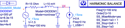
Fig. 10: The circuit R-L-diode circuit is excited with a small-signal current source at the diode.

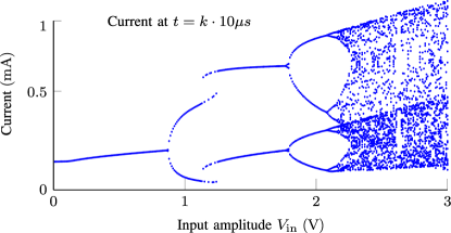
Fig. 11: The bifurcation diagram of the R-L-diode circuit shows that a period-doubling occurs for input amplitudes higher than $0.8\leavevmode\nobreak\ \mathrm{V}$.

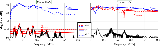
Fig. 12: The results of the stability analysis of $Z_{mn}^{\left[-1\right]}\!\left(j\omega\right)$ $Z_{mn}^{\left[0\right]}\!\left(j\omega\right)$ and $Z_{mn}^{\left[+1\right]}\!\left(j\omega\right)$ in the two HB simulations show that, for $V_{\mathrm{in}}=0.5\leavevmode\nobreak\ \mathrm{V}$, the orbit is stable, but for $V_{\mathrm{in}}=1.5\leavevmode\nobreak\ \mathrm{V}$, the orbit is unstable. The interpolation error in shown with ( ).

The final example in this paper shows that the stability analysis can also be used to determine the stability of HB simulations of the R-L-diode circuit shown in Fig. 12. The circuit is based on [28], but a realistic diode model was used to represent the diode in the circuit instead of the three equations provided in the original paper.

The circuit is excited by a single-tone voltage source with an amplitude $V_{\mathrm{in}}$ and a frequency of $100\leavevmode\nobreak\ \mathrm{kHz}$. Because the diode has a transit-time of $4\leavevmode\nobreak\ \mathrm{\mu s}$, the circuit generates period-doubling solutions starting from sufficiently high amplitudes $V_{\mathrm{in}}$. For even higher $V_{\mathrm{in}}$, the circuit will create chaotic solutions.

To visualise this behaviour, a bifurcation diagram is constructed using time-domain simulations in the same way as is described in [28]: For every value of $V_{\mathrm{in}}$, 1030 periods of $100\leavevmode\nobreak\ \mathrm{kHz}$ are simulated and the final 30 periods are sampled every $\nicefrac{{1}}{{100\leavevmode\nobreak\ \mathrm{kHz}}}$. If the circuit solution is periodic with the same period as the input source, all 30 sampled points will fall on top of each-other. If a period-doubling occurs in the circuit, two different values will be obtained.

The obtained bifurcation diagram for our R-L-diode example is shown in Fig. 12. It is clear that a period-doubling occurs for $V_{\mathrm{in}}$ higher than $0.8\leavevmode\nobreak\ \mathrm{V}$. Starting from $1.8\leavevmode\nobreak\ \mathrm{V}$ the period quadruples. For the highest input amplitudes, a chaotic solution is obtained.

If this R-L-diode circuit is simulated with HB, the circuit solution is constrained to harmonics of $100\leavevmode\nobreak\ \mathrm{kHz}$. For input amplitudes higher than $0.8\leavevmode\nobreak\ \mathrm{V}$, where the circuit wants to go to a period-doubling solution, the constrained HB solution will be locally unstable.

We run two HB simulations on this circuit. Both HB simulations have a base frequency of $100\leavevmode\nobreak\ \mathrm{kHz}$ and an order of 10. In the first simulation, $V_{\mathrm{in}}$ is set to $0.5\leavevmode\nobreak\ \mathrm{V}$, which will result in a stable orbit. The second simulation has a $V_{\mathrm{in}}$ of $1.5\leavevmode\nobreak\ \mathrm{V}$, which will cause the orbit to be unstable.

The frequency response of the circuit around the HB solution is obtained with a mixer-like simulation, as explained in the introduction of this paper. The small-signal excitation was swept in both cases on a linear frequency grid starting from $(1\leavevmode\nobreak\ \mathrm{kHz}+1\leavevmode\nobreak\ \mathrm{Hz})$ up to $(2\leavevmode\nobreak\ \mathrm{MHz}+1\leavevmode\nobreak\ \mathrm{Hz})$ in $1\leavevmode\nobreak\ \mathrm{kHz}$ steps. The $1\leavevmode\nobreak\ \mathrm{Hz}$ was added to the start and stop values of the sweep to avoid overlap with the tones of the HB simulation.

The mixer-like simulation in ADS uses Single-Sideband (SSB) current excitations $i\left(t\right)=e^{j\omega t}$, which causes the obtained frequency responses $Z_{mn}^{\prime\left[b\right]}\left(j\omega\right)$ with $b\neq 0$ to be non-Hermitian:

$$Z_{mn}^{\prime\left[b\right]}\left(j\omega\right)\neq\overline{Z_{mn}^{\prime\left[b\right]}\left(-j\omega\right)}$$

An alternative representation can make $Z_{mn}^{\prime\left[b\right]}\left(j\omega\right)$ Hermitian by transferring to a sine and cosine basis from the exponential basis [29, 30]

$$Z_{mn}^{\left[b\right]}\!\left(j\omega\right) =\frac{1}{2}\left[Z_{mn}^{\prime\left[b\right]}\left(j\omega\right)+Z_{mn}^{\prime\left[-b\right]}\left(j\omega\right)\right]$$

$$Z_{mn}^{\left[-b\right]}\!\left(j\omega\right) =\frac{j}{2}\left[Z_{mn}^{\prime\left[b\right]}\left(j\omega\right)-Z_{mn}^{\prime\left[-b\right]}\left(j\omega\right)\right]$$

$Z_{mn}^{\left[-1\right]}\!\left(j\omega\right)$ $Z_{mn}^{\left[0\right]}\!\left(j\omega\right)$ and $Z_{mn}^{\left[+1\right]}\!\left(j\omega\right)$ are then analysed with the stable/unstable projection method. The results are shown in Fig. 12. The HB solution obtained for $V_{\mathrm{in}}=0.5\leavevmode\nobreak\ \mathrm{V}$ is clearly stable: its unstable part is more than $70\leavevmode\nobreak\ \mathrm{dB}$ smaller than its stable part.

In the case for $V_{\mathrm{in}}=1.5\leavevmode\nobreak\ \mathrm{V}$, the solution is clearly unstable as the unstable part lies far above the stable part of the frequency response. Note that the lowest-frequency peak in the unstable part is located around $50\leavevmode\nobreak\ \mathrm{kHz}$ and that copies of the resonance are found at $150\leavevmode\nobreak\ \mathrm{kHz}$, $250\leavevmode\nobreak\ \mathrm{kHz}$,… This behaviour is to be expected and indicates that the circuit wants to go to a period-doubling solution.

During the stability analysis of a periodic orbit, the unstable part will contain both the unstable base pole and all its higher-order copies. The unstable part will be simple, just like in the small-signal case, and it will be possible to approximate it by a finite set of base poles. Due to the infinite amount of higher-order copies however, it will not be possible to approximate it by a low-order rational approximation as is the case in the stability analysis of a DC solution.

IV Conclusion

This paper introduces a closed-loop local stability analysis without using a rational approximation. Instead, the impedance functions are split into a stable and unstable part by projecting onto an orthogonal basis. Transforming the problem to the unit disc allows to calculate this projection with the FFT which makes the projection-based stability analysis very fast. In a small-signal stability analysis, once the unstable part is obtained, a low-order rational model can be used to find the unstable poles in the circuit.

Due to the model-free nature of the proposed method, it is a very simple method to use: no choice of model order or approximation error needs to be made. The only requirements of the projection-based stability analysis are that the frequency responses are sampled on a sufficiently dense frequency grid and that the maximum frequency of the simulations is large enough. When the circuit impedance is simulated on a too coarse frequency grid, a large interpolation error is introduced in the results. The level of this interpolation error can easily be determined and used to improve the accuracy of the method.

Once the stable and unstable parts of the impedance are obtained with a sufficiently low interpolation error, the obtained unstable part can be compared to the interpolation error to determine whether it is significant or not. From experience, we found that, when the unstable part lies more than $20\leavevmode\nobreak\ \mathrm{dB}$ above the interpolation error level, the circuit can be considered unstable. Further work is to be done towards automated decision making regarding stability.

The stable/unstable projection has been successfully applied to both the stability analysis of DC and large-signal solutions of RF circuits.

Appendix A On local rational approximation

Due to the presence of distributed elements in microwave circuits it is impossible to obtain a rational model of the impedances of the circuit over the full simulated frequency range. In a small frequency band however, it is possible to obtain a good low-order rational approximation of the impedance. This is the basis of pole-zero based stability analysis.

It is however not guaranteed that the poles of the local model correspond to the poles of the global model. We will demonstrate this in this appendix using an simple example without distributed elements.

$$Z\left(s\right)=\frac{\begin{array}[]{c}-228.5s^{14}-153.7s^{13}-875.2s^{12}-550.2s^{11}-1364.9s^{10}-789.9s^{9}\\ -1118.6s^{8}-584.2s^{7}-520.9s^{6}-239.2s^{5}-140.7s^{4}-54.7s^{3}-21.4s^{2}-5.9s-1\end{array}}{\nicefrac{{\left(s+5\right)^{15}}}{{9.9281\cdot 10^{10}}}}$$ (12)

Consider the artificial example in equation (12). All poles of this rational function lie in $s=-5$, so $Z(s)$ is stable. In the frequency band $[-1,1]$ however, the FRF of this stable rational function closely resembles an unstable FRF (Figure 13)

To verify whether the global poles are obtained with a local model, we estimate a local rational model on 1000 frequency points on the interval $\omega\in[-0.6,0.6]$ using vector fitting [31]. The model order for the local model is not known in advance, so it is swept from 2 to 11. The maximum of the phase error of the obtained fit is shown in Figure 15. Starting from model order 8, the phase error lies below $10^{-3}$ degrees so the fit can be considered sufficiently good for stability analysis [17].

The obtained local model is unstable however. In fact, an unstable local model is obtained for all model, which shows that the poles of a local model do not necessarily correspond to the poles of the underlying impedance. This is an artificial example of course, but the example indicates that the use of local lower-order models to determine the stability could lead to misleading results.

Fig. 13: FRF used in Appendix A. The FRF is stable, but resembles an unstable FRF in the interval [-1,1]. Using a local model of this FRF might result in false positives during stability analysis.

Fig. 14: Maximum phase error as a function of the model order obtained when estimating a local model in the range $\omega\in[-0.6,0.6]$ of the stable impedance (12).

Fig. 15: The obtained poles and zeroes for model order 8. The model was estimated using data in the interval $\omega\in[-0.6,0.6]$. The red circle indicates all points $s$ in the complex plane for which $\left|s\right|<0.6$.

Appendix B Mapping of the basis functions onto the unit disc

Applying transform (9) to the basis functions of the complex plane (5) yields the following:

$$B_{k}^{\mathrm{disc}}\left(z\right)=\sqrt{\pi\alpha}\frac{2}{z-1}B_{k}\left(\alpha\frac{1+z}{1-z}\right)\\ =-\sqrt{\pi\alpha}\frac{2}{z-1}\sqrt{\frac{\alpha}{\pi}}\frac{\left(\alpha\frac{1+z}{1-z}-\alpha\right)^{k}}{\left(\alpha\frac{1+z}{1-z}+\alpha\right)^{k+1}}=z^{k}$$

Adam Cooman was born in Belgium in 1989. He graduated as an Electrical Engineer in Electronics and Information Processing in 2012 at Vrije Universiteit Brussel (VUB) and obtained his Ph.D at the Department ELEC of the VUB in December 2016. Now, Adam is part of the APICS team at INRIA, Sophia Antipolis, France. His main interests are the design of Electronic circuits, from low frequencies up to the microwave frequencies.

Fabien Seyfert graduated from the “Ecole superieure des Mines” (Engineering School) in St Etienne (France) in 1993 and received his Ph.D in mathematics in 1998. From 1998 to 2001 he was with Siemens (Munich, Germany) as a researcher specialized in discrete and continuous optimization methods. Since 2002 he occupies a full research position at INRIA (French agency for computer science and control, Nice, France). His research interest focuses on the conception of effective mathematical procedures and associated software for problems from signal processing including computer aided techniques for the design and tuning of microwave devices.

Martine Olivi was born in France, in 1958. She got the engineer’s degree from Ecole des Mines de St-Etienne, France, and the PhD degree in Mathematics from Université de Provence, Marseille, France, in 1983 and 1987 respectively. Since 1988, she is with the Institut National de Recherche en Informatique et Automatique (INRIA), Sophia Antipolis, France. Her research interests include: rational approximation, parametrization of linear multivariable systems, Schur analysis, identification and design of resonant systems. Detailed information and publications are available at www-sop.inria.fr/members/Martine.Olivi

Sylvain Chevillard was born in Paris, France, in 1983. He received his Ph.D. in computer science from Université de Lyon - École Normale Supérieure de Lyon in 2009. He is Chargé de recherche (junior researcher) at Inria Sophia Antipolis, France. Some of his research interests are reliable computing, approximation theory, computer algebra, inverse problems.

Laurent Baratchart received his Docteur Ingénieur degree from Ecole des Mines de Paris in 1982 (advisor: Y. Rouchaleau) and his Thèse d’état in Mathematics from the University of Nice in 1987 (advisor: A. Galligo). He was the head of INRIA’s project team MIAOU (Mathematics and Informatics in Automatic control and Optimization for the User) from 1988 to 2003 and is currently the head of the project team APICS (Analysis of Problems of Inverse type in Control and Signal processing) at INRIA Sophia-Antipolis since 2004. His main interests lie with Complex and Harmonic Analysis, Inverse Problems, as well as System and Circuit Theory.

References

- [1] A. Suarez, “Check the stability: Stability analysis methods for microwave circuits,” Microwave Magazine, IEEE, vol. 16, no. 5, pp. 69–90, June 2015.
- [2] A. Suarez and R. Quere, Stability analysis of nonlinear microwave circuits. Artech House, 2002.
- [3] J. Jugo, J. Portilla, A. Anakabe, A. Suarez, and J. Collantes, “Closed-loop stability analysis of microwave amplifiers,” Electronics Letters, vol. 37, no. 4, pp. 226–228, Feb 2001.
- [4] J. Collantes, I. Lizarraga, A. Anakabe, and J. Jugo, “Stability verification of microwave circuits through floquet multiplier analysis,” in Circuits and Systems, 2004. Proceedings. The 2004 IEEE Asia-Pacific Conference on, vol. 2, Dec 2004, pp. 997–1000 vol.2.
- [5] J. Partington, Linear operators and linear systems, ser. Student texts. London Math. Soc., 2004, no. 60.
- [6] L. Baratchart, S. Chevillard, and F. Seyfert. (2014) On transfer functions realizable with active electronic components. hal-01098616. Inria Sophia Antipolis. [Research Report] RR-8659.
- [7] W. Rudin, Real and Complex analysis. Mc Graw-Hill, 1982.
- [8] G. A. Baker and P. Graves-Morris, Padé Approximants, ser. Encyclopedia of Mathematics and its Applications. Cambridge University Press, 1996, vol. 59.
- [9] A. A. Gonchar and E. Saff, Eds., Spurious Poles in Diagonal Rational Approximation, ser. Series in Computational Mathematics, vol. 19. New York: Springer, 1992, in Progress in Approximation Theory.
- [10] H. Stahl, “Spurious poles in padé approximation,” Journal of Computational and Applied Mathematics, no. 99, 1998.
- [11] S. G. P. Gonnet and L. N. Trefethen, “Robust padé approximation via svd,” SIAM Rev., vol. 55, pp. 101–117, 2013.
- [12] B. Beckermann and A. Matos, “Algebraic properties of robust padé approximants,” Jour. Approx. Theory, vol. 190, pp. 91–115, 2015.
- [13] A. Lefteriu and A. C. Antoulas, “On the convergence of the vector fitting algorithm,” IEEE Transactions on Microwave Theory and Techniques, vol. 61, no. 4, 2013.
- [14] L. Ljung, System identification: Theory for the user. Prentice–Hall, 1987.
- [15] A. Anakabe, N. Aylloon, J. Collantes, A. Mallet, G. Soubercaze-Pun, and K. Narendra, “Automatic pole-zero identification for multivariable large-signal stability analysis of rf and microwave circuits,” in Microwave Conference (EuMC), 2010 European, Sept 2010, pp. 477–480.
- [16] AMCAD. engineering, STAN tool - Stability Analysis.
- [17] I. Mallet, A. Ankabe, G. Soubercaze-Pun, and J.-M. Collantes, “Automation of the zero-pole identification methods for the stab analysis of microwave active circuits,” U.S. Patent 8,407,637 B2, 2013.
- [18] M. van Heijningen, A. P. de Hek, F. E. van Vliet, and S. Dellier, “Stability analysis and demonstration of an x-band gan power amplifier mmic,” in 2016 11th European Microwave Integrated Circuits Conference (EuMIC), Oct 2016, pp. 221–224.
- [19] N. Otegi, A. Anakabe, J. Pelaz, J. Collantes, and G. Soubercaze-Pun, “Experimental characterization of stability margins in microwave amplifiers,” Microwave Theory and Techniques, IEEE Transactions on, vol. 60, no. 12, pp. 4145–4156, Dec 2012.
- [20] J. Collantes, N. Otegi, A. Anakabe, N. Ayllon, A. Mallet, and G. Soubercaze-Pun, “Monte-carlo stability analysis of microwave amplifiers,” in Wireless and Microwave Technology Conference (WAMICON), 2011 IEEE 12th Annual, April 2011, pp. 1–6.
- [21] N. Ayllon, J. M. Collantes, A. Anakabe, I. Lizarraga, G. Soubercaze-Pun, and S. Forestier, “Systematic approach to the stabilization of multitransistor circuits,” IEEE Tran. on Microwave Theory and Techniques, vol. 59, no. 8, pp. 2073–2082, 2011.
- [22] M. Olivi, F. Seyfert, and J.-P. Marmorat, “Identification of microwave filters by analytic and rational h2 approximation,” Automatica, vol. 10, Februari 2013.
- [23] K. Hoffman, Banach spaces of analytic functions, ser. Prentice-Hall series in modern analysis. Prentice-Hall, 1962.
- [24] J. P. Marmorat and M. Olivi, “RARL2: a Matlab based software for rational approximation,” http://www-sop.inria.fr/apics/RARL2/rarl2.html, 2004.
- [25] S. Kung, “A new identification and model reduction algorithm via singular value decomposition,” in Proceedings of the 12th Asilomar Conference on Circuits, Systems and Computers, 1978, pp. 705–714.
- [26] I. Markovsky, Low Rank Approximation: Algorithms, Implementation, Applications. Springer, 2012. [Online]. Available: http://homepages.vub.ac.be/~imarkovs/book.html
- [27] D. Floriot, H. Blanck, D. Bouw, F. Bourgeois, M. Camiade, L. Favede, M. Hosch, H. Jung, B. Lambert, A. Nguyen, K. Riepe, J. Splettstosse, H. Stieglauer, J. Thorpe, and U. Meiners, “New qualified industrial algan/gan hemt process: Power performances amp; reliability figures of merit,” in 2012 7th European Microwave Integrated Circuit Conference, Oct 2012, pp. 317–320.
- [28] A. Azzouz, R. Duhr, and M. Hasler, “Transition to chaos in a simple nonlinear circuit driven by a sinusoidal voltage source,” IEEE Transactions on Circuits and Systems, vol. 30, no. 12, pp. 913–914, Dec 1983.
- [29] E. Louarroudi, “Frequency domain measurement and identification of weakly nonlinear time-periodic systems,” Ph.D. dissertation, Vrije Universiteit Brussel (VUB), 2014.
- [30] H. Sandberg, E. Mollerstedt, and Bernhardsson, “Frequency-domain analysis of linear time-periodic systems,” Automatic Control, IEEE Transactions on, vol. 50, no. 12, pp. 1971 – 1983, dec. 2005.
- [31] B. Gustavsen and A. Semlyen, “Rational approximation of frequency domain responses by vector fitting,” Power Delivery, IEEE Transactions on, vol. 14, no. 3, pp. 1052–1061, Jul 1999.