An approach to calculation of mass spectra and two-photon decays of $c\overline{c}$ mesons in the framework of Bethe-Salpeter Equation

¹Department of Physics, Chandigarh University, Mohali-140413, India
² Department of Physics, Addis Ababa University, P.O.Box 1176, Addis Ababa, Ethiopia

Abstract
In this work we calculate the mass spectrum of charmonium for $1P,...,3P$ states of $0^{++}$ , $1^{++}$, as well as for $1S,...,4S$ states of $0^{-+}$, and $1S,...,5D$ states of $1^{--}$ along with the two-photon decay widths of ground and first excited state of $0^{++}$ quarkonia for the process, $O^{++}\rightarrow\gamma\gamma$ in the framework of a QCD motivated Bethe-Salpeter Equation. In this $4\times 4$ BSE framework, the coupled Salpeter equations are first shown to decouple for the confining part of interaction, under heavy-quark approximation, and analyically solved, and later the one-gluon-exchange interaction is perturbatively incorporated leading to mass spectral equations for various quarkonia. The analytic forms of wave functions obtained are used for calculation of two-photon decay widths of $\chi_{c0}$. Our results are in reasonable agreement with data (where ever available) and other models.

Key words: Bethe-Salpeter equation, Covariant Instantaneous Ansatz, Mass spectral equation, charmonium, bottomonium

PACS: 12.39.-x, 11.10.St , 21.30.Fe , 12.40.Yx , 13.20.-v

1 Introduction

An important role in applications of Quantum Chromodynamics (QCD) to hadronic physics is played by charmonium ($c\overline{c}$) and bottomonium ($b\overline{b}$), which are built up of a heavy quark and heavy anti-quark. By definition, heavy quark has a mass $m$, which is large in comparison to the typical hadronic scale, $\Lambda_{QCD}$. Quarkonia are characterized by at least three widely separated scales [1]: the hard scale (the mass $m$ of heavy quarks), the soft scale (relative momentum $q\sim mv)$, and the ultra soft scale (typical kinetic energy, $E\sim mv^{2}$ of heavy quark and anti-quark). The appearance of all these scales in the dynamics of heavy quarkonium makes its quantitative study extremely difficult. Quarkonium systems are crucially important to improve our understanding of QCD. They probe all the energy regions of QCD from hard region, where perturbative QCD dominates, to the low energy region, where non-perturbative effects dominate. Quarkonium states are thus a unique laboratory where our understanding of non-perturbative QCD may be tested.

There has a been a renewed interest in recent years in spectroscopy of these heavy hadrons in charm and beauty sectors, which was primarily due to experimental facilities the world over such as BABAR, Belle, CLEO, DELPHI, BES etc. [2, 3, 4, 5, 6], which have been providing accurate data on $c\overline{c}$, and $b\overline{b}$ hadrons with respect to their masses and decays. In the process many new states have been discovered such as $\chi_{b0}(3P)$, $\chi_{c0}(2P),X(3915),X(4260),X(4360),X(4430),X(4660)$ [6]. The data strongly suggests that among new resonances may be exotic four-quark states, or hybrid states with gluonic degrees of freedom in addition to $c\overline{c}$ pair, or loosely bound states of heavy hadrons, i.e. charmonium molecules. Further, there are also open questions about the quantum number assignments of some of these states such as $X(3915)$ (as to whether it is $\chi_{c0}(2P)$ or $\chi_{c2}(2P)$ [7, 8]). Thus charmonium offers us intriguing puzzles.

However, since the mass spectrum and the decays of all these bound states of heavy quarks can be tested experimentally, theoretical studies on them may throw valuable insight about the heavy quark dynamics and lead to a deeper understanding of QCD further. Studies on mass spectrum of these hadrons is particularly important, since it throws light on the $Q\overline{Q}$ potential, since the long range confinement potential can not be derived from QCD alone. Further, though these states appear to be simple, however, their production mechanism is still not properly understood. These mesons are involved in a number of reactions which are of great importance for study of Cabibbo-Kobayashi-Maskawa (CKM) matrix and CP violation. In this paper we also study the two-photon decays of scalar quarkonia, $\chi_{c0}$. These decays are sensitive probes of quarkonium wave functions.

The non-perturbative approaches, such as Effective field theory [9], Lattice QCD [10, 11, 12], Chiral perturbation theory [13], QCD sum rules [14, 15], N.R.QCD [16], Bethe-Salpeter equation (BSE) [17, 18, 19, 20, 21, 22, 23, 24, 25, 26], and potential models [27, 28, 29] deal have been employed to study heavy quarkonia. Recent progress in understanding of non-relativistic field theories make it possible to go beyond phenomenological models, and for the first time face the possibility of providing unified description of all aspects of heavy quarkonium physics. This allows us to use quarkonium as a bench mark for understanding of QCD, and for precise determination of Standard Model parameters (e.g. heavy quark masses, QCD coupling constant, $\alpha_{s}$), and for new physics searches.

All this opens up new challenges in theoretical understanding of heavy hadrons and also provide an important tool for exploring the structure of these simplest bound states in QCD and for studying the non-perturbative (long distance) behavior of strong interactions.

In present work, we do the full mass spectral problem of charmonium for $1P,...,3P$ states of $0^{++}$ , $1^{++}$ , as well as for $1S,...,4S$ states of $0^{-+}$, and $1^{--}$ along with the two-photon decay widths of ground and first excited state of scalar quarkonia, $\chi_{c0}$ for the process, $O^{++}\rightarrow\gamma\gamma$ in the framework of a QCD motivated Bethe-Salpeter Equation under Covariant Instantaneous Ansatz (CIA), employing the full BS kernel comprising both, the long-range confinement, and the short range one-gluon-exchange (coulomb) interactions.

We do understand that in $Q\overline{Q}$ quarkonia, the constituents are close enough to each other to warrant a more accurate treatment of the coulomb term. Though for $b\overline{b}$ systems, the coulomb term will be extremely dominant in comparison to confining term, and should not be treated perturbatively. However, seeing our mass spectral results for $c\overline{c}$ systems, it may not be so unreasonable to treat the coulomb term perturbatively for $c\overline{c}$ systems. This is specially so for orbital excitations of these states, where the centrifugal effects [34] ensure that the $c-\overline{c}$ separation is large enough to feel the effect of confining term more strongly than the coulomb term. We further wish to state that some of earlier works [34, 35, 36] have treated the OGE(coulomb) term perturbatively for charmed mesons and baryons, while some works [37, 38] did not take into account the importance of coulomb term for heavy quarkonium systems.

Thus, in the present paper, the coupled Salpeter equations for scalar ($0^{++}$), and axial vector ($1^{++}$) quarkonia are first shown to decouple for the confining part of interaction, under heavy-quark approximation, and the analytic forms of mass spectral equations are worked out, which are then solved in approximate harmonic oscillator basis to obtain the unperturbed wave functions for various states of these quarkonia. We then incorporate the one-gluon-exchange perturbatively into the unperturbed spectral equation, and obtain the full spectrum. The wave functions of scalar ($0^{++}$) quarkonia, are then used to calculate their two-photon decay widths. We further extend the mass spectral calculations of pseudoscalar ($0^{-+}$), and vector ($1^{--}$) quarkonia in [30] with the perturbative inclusion of one-gluon-exchange effects. The approximations used in this analytic treatment of the confining interaction are shown to be fully under control. This work is an improvement on our earlier work [30] on mass spectral problem for pseudoscalar and vector states of quarkonia on lines of some of the earlier works [31, 32, 33], where we used only the confining interaction.

A quarkonium state is classified by quantum numbers, $J^{PC}$, where $J=L+S$, parity, $P=(-1)^{L+1}$, and charge conjugation, $C=(-1)^{L+S}$. With this classification, while the lowest states, $l=0$ are present in $0^{-+}$ (pseudoscalar), the lowest state ($l=0$), and the second orbitally excited $(l=2)$ state are present in $1^{--}$ (vector) quarkonia. However, the first orbitally excited ($l=1$) states are present in $0^{++}$ (scalar) and $1^{++}$ (axial-vector) quarkonia. The same holds true for their radial excitations.

This paper is organized as follows: Section 2, deals with the mass spectral calculations of ground and excited states of $0^{++}$ quarkonia. Section 3 deals with the mass spectral calculation of ground and excited states of $0^{-+}$, and $1^{--}$ quarkonia, while Section 4 deals with the mass spectral calculations of ground and excited states of $1^{++}$ quarkonia. Section 5 deals with the calculation of two-photon decay widths of $\chi_{c0}$. Section 6 deals with numerical results and discussions.

2 Mass spectra of scalar quarkonia

In the center of mass frame, where $q_{\mu}=(\hat{q},i0)$, we can write the general decomposition of the instantaneous BS wave function for scalar mesons $(J^{pc}=0^{++})$, of dimensionality $M$ as

$$\psi(\hat{q})=Mf_{1}(\hat{q})-i\not{P}f_{2}(\hat{q})-i\not{\hat{q}}f_{3}(\hat{q})-\frac{2\not{P}\not{\hat{q}}}{M}f_{4}(\hat{q}).$$ (1)

where it can be shown by use of a power counting rule proposed in [23, 25] that the Dirac structures associated with the amplitudes $f_{1}$ and $f_{2}$ are leading, and will contribute maximum to calculation of any scalar meson observable, while those associated with $f_{3}$, and $f_{4}$ are sub-leading. We now use the two constraint equations $\psi^{+-}(\hat{q})=\psi^{-+}=0$ in the 3D Salpeter equations, Eq.(16) of [30], to reduce the four scalar functions into two independent scalar wave functions. For equal mass system, these two equations are reduced to

$$f_{1}(\hat{q})=\frac{-\hat{q}^{2}f_{3}(\hat{q})}{Mm};$$

$$f_{2}(\hat{q})=0.$$ (2)

Applying the above constraint conditions in Eq.(2) to wave function in Eq.(1), we rewrite the relativistic wave function of the state $(0^{++})$ in the form

$$\psi(\hat{q})=\bigg{[}\frac{-\hat{q}^{2}}{m}-i\not{\hat{q}}\bigg{]}f_{3}(\hat{q})-\frac{2\not{P}\not{\hat{q}}}{M}f_{4}(\hat{q}).$$ (3)

Here, it is to be noted that by use of the above constraint equations, we have reexpressed $f_{1}$ in terms of $f_{3}$. Thus, the Instantaneous BS wave function of $(0^{++})$ state is determined by only two independent functions, $f_{3}$ and $f_{4}$. Putting the wave function in Eq.(3) above, along with the projection operators defined in Eq.(13) of [30], into the first two Salpeter equations, Eq.(16) of [30], and by taking the trace on both sides, we obtain the equations:

$$(M-2\omega)\bigg{[}f_{3}(\hat{q})+\frac{2mf_{4}(\hat{q})}{\omega}\bigg{]}=\frac{1}{\omega^{2}\hat{q}^{2}}\int\frac{d^{3}\hat{q}}{(2\pi)^{3}}K(\hat{q},\hat{q}^{\prime})\bigg{[}\hat{q}^{2}\hat{q}^{\prime 2}f_{3}(\hat{q}^{\prime})-m^{2}\hat{q}.\hat{q}^{\prime}f_{3}(\hat{q}^{\prime})-2m\omega\hat{q}.\hat{q}^{\prime}f_{4}(\hat{q}^{\prime})\bigg{]}$$

$$(M+2\omega)\bigg{[}f_{3}(\hat{q})-\frac{2mf_{4}(\hat{q})}{\omega}\bigg{]}=\frac{1}{\omega^{2}\hat{q}^{2}}\int\frac{d^{3}\hat{q}}{(2\pi)^{3}}K(\hat{q},\hat{q}^{\prime})\bigg{[}-\hat{q}^{2}\hat{q}^{\prime 2}f_{3}(\hat{q}^{\prime})+m^{2}\hat{q}.\hat{q}^{\prime}f_{3}(\hat{q}^{\prime})-2m\omega\hat{q}.\hat{q}^{\prime}f_{4}(\hat{q}^{\prime})\bigg{]}$$ (4)

Solution of these equations needs information about the BS kernel, $K(\hat{q},\hat{q}^{\prime})$ [25, 30], which is taken to be one-gluon exchange like as regards the colour ($\frac{1}{4}\vec{\lambda}_{1}.\vec{\lambda}_{2}$) and spin ($\gamma_{\mu}\ \bigotimes\gamma_{\mu}$) dependence, and has a scalar part $V(\hat{q},\hat{q}^{\prime})$, written as,

$$V(\hat{q},\hat{q}^{\prime})=\frac{4\pi\alpha_{s}}{(q-q^{\prime})^{2}}+\frac{3}{4}\omega^{2}_{q\bar{q}}\int d^{3}\vec{r}[\kappa r^{2}-\frac{C_{0}}{\omega_{0}^{2}}]e^{i(\hat{q}-\hat{q}^{\prime}).\vec{r}}=V_{OGE}+V_{c}.$$ (5)

Thus, the scalar part $V(\hat{q},\hat{q}^{\prime})$ of the kernel involves both the OGE term $V_{OGE}$, arising from the one-gluon exchange, as well as the confining term, $V_{c}$. We first ignore the $V_{OGE}$ term, and work only with the confining part, $V_{c}$ in Eq.(5), and write Eqs.(4) as,

$$(M-2\omega)\bigg{[}f_{3}(\hat{q})+\frac{2mf_{4}(\hat{q})}{\omega}\bigg{]}=\frac{\Theta_{s}}{\omega^{2}\hat{q}^{2}}\int\frac{d^{3}\hat{q}^{\prime}}{(2\pi)^{3}}V_{c}(\hat{q},\hat{q}^{\prime})\bigg{[}\hat{q}^{2}\hat{q}^{\prime 2}f_{3}(\hat{q}^{\prime})-m^{2}\hat{q}.\hat{q}^{\prime}f_{3}(\hat{q}^{\prime})-2m\omega\hat{q}.\hat{q}^{\prime}f_{4}(\hat{q}^{\prime})\bigg{]}$$

$$(M+2\omega)\bigg{[}f_{3}(\hat{q})-\frac{2mf_{4}(\hat{q})}{\omega}\bigg{]}=\frac{\Theta_{s}}{\omega^{2}\hat{q}^{2}}\int\frac{d^{3}\hat{q}^{\prime}}{(2\pi)^{3}}V_{c}(\hat{q},\hat{q}^{\prime})\bigg{[}-\hat{q}^{2}\hat{q}^{\prime 2}f_{3}(\hat{q}^{\prime})+m^{2}\hat{q}.\hat{q}^{\prime}f_{3}(\hat{q}^{\prime})-2m\omega\hat{q}.\hat{q}^{\prime}f_{4}(\hat{q}^{\prime})\bigg{]},$$ (6)

where the spin dependence of the interaction is contained in the factor, $\Theta_{S}=\gamma_{\mu}\psi(\widehat{q})\gamma_{\mu}$. The scalar part of the confining potential (that involves the colour factor $\frac{1}{2}\vec{\lambda}_{1}.\frac{1}{2}\vec{\lambda}_{2}=-\frac{4}{3}$), is taken to be [30] $V_{c}(\hat{q},\hat{q^{\prime}})=\overline{V}_{c}\delta^{3}(\hat{q}-\hat{q}^{\prime})$, where $\overline{V}_{c}(\hat{q},\hat{q^{\prime}})=\omega_{q\bar{q}}^{2}(2\pi)^{3}\big{[}\kappa\vec{\nabla}_{\hat{q}}^{2}+\frac{C_{0}}{\omega_{0}^{2}}\big{]}$, and $\kappa=(1-A_{0}M^{2}\overrightarrow{\nabla}^{2}_{\hat{q}})^{-1/2}$. Here $\overline{V_{c}}$ is the part of $V_{c}$ without the delta function. To handle these equations, we first integrate these equations over $d^{3}\widehat{q}^{\prime}$, performing the delta function integration that arises due to presence of $V_{c}(\hat{q},\hat{q^{\prime}})$ in the integrand, and get two coupled algebraic equations with $\overline{V}(\widehat{q})$ on RHS. To decouple them, we first add them. Then we subtract the second equation from the first equation, and get two algebraic equations which are still coupled. Then from one of the two equations so obtained, we eliminate $f_{3}(\hat{q})$ in terms of $f_{4}(\hat{q})$, and plug this expression for $f_{3}(\hat{q})$ in the second equation of the coupled set so obtained, to get a decoupled equation in $f_{4}(\hat{q})$. Similarly, we eliminate $f_{4}(\hat{q})$ from the second equation of the set of coupled algebraic equations in terms of $f_{3}(\hat{q})$, and plug it into the first equation to get a decoupled equation entirely in $f_{3}(\hat{q})$. Thus, we get two identical decoupled equations, one entirely in $f_{3}(\hat{q})$, and the other that is entirely in, $f_{4}(\hat{q})$. The calculation up to this point is without any approximation. However, we notice that if we employ the approximation, $\omega\approx m$ on RHS of the two algebraic equations (this is justified since in the confinement region, the relative momentum between heavy quarks in the bound state can be considered small, since the heavy-quark is expected to move with non-relativistic speeds (see Ref.[39]), and these quarks can be treated as almost on mass shell), these decoupled equations can be expressed as:

$$\bigg{[}\frac{M^{2}}{4}-m^{2}-\widehat{q}^{2}\bigg{]}f_{3}(\hat{q})=-m\Theta_{s}\overline{V}_{c}f_{3}(\hat{q})+\frac{\Theta_{s}^{2}\overline{V}_{c}^{2}f_{3}(\widehat{q})}{4}$$

$$\bigg{[}\frac{M^{2}}{4}-m^{2}-\widehat{q}^{2}\bigg{]}f_{4}(\hat{q})=-m\Theta_{s}\overline{V}_{c}f_{4}(\hat{q})+\frac{\Theta_{s}^{2}\overline{V}_{c}^{2}f_{4}(\widehat{q})}{4},$$ (7)

We see that we get two identical decoupled equations which resemble the harmonic oscillator equations, but for the term involving $\overline{V}_{c}^{2}$ on the right side of these equations.

We wish to mention that in recent studies on mass spectra of pseudoscalar and vector quarkonia [30], it was seen that good agreement with data on masses and various decay constants/decay widths of ground and excited states of $\eta_{c},\eta_{b},J/\Psi$, and $\Upsilon$ is obtained for input parameters, $C_{0}=0.175$, $\omega_{0}=0.160$ GeV., $\Lambda=0.200$ GeV., and $A_{0}=0.01$, along with the input quark masses $m_{c}=1.490$ GeV. With these numerical values of input parameters, we try to determine the numerical values of $\Omega_{S}=m\Theta_{S}\omega^{2}_{q\bar{q}}$, and $\Omega_{S}^{\prime}=\frac{\Theta_{S}^{2}}{4}\omega^{4}_{q\bar{q}}$ associated with the terms involving $\overline{V}_{c}$ and $\overline{V}_{c}^{2}$ respectively, for scalar mesons $\chi_{c}$ and $\chi_{b}$ in RHS of Eqs.(12), and their percentage ratio in Table 1 below, where it can be seen that $\omega_{q\bar{q}}^{4}\ll\omega_{q\bar{q}}^{2}$ and hence the second term on RHS of Eqs.(7) contributes $<1\%$, than the first term on RHS of this equation for $c\overline{c}$, so that it can be dropped.

	$\Omega_{S}$	$\Omega_{S}^{\prime}$	$\frac{\Omega_{S}^{\prime}}{\Omega_{S}}\%$
$\chi_{c0}$	0.0558	0.000356	0.638

Table 1: Numerical values of coefficients, $\Omega_{S}=m\Theta_{S}\omega^{2}_{q\bar{q}}$, and $\Omega_{S}^{\prime}=\frac{\Theta_{S}^{2}}{4}\omega^{4}_{q\bar{q}}$ associated with the terms involving $\overline{V}_{c}$ and $\overline{V}_{c}^{2}$ respectively, for scalar mesons $\chi_{c}$ in RHS of Eqs.(7), and their percentage ratio for the input parameters of our model mentioned above.

Thus the RHS of both equations in Eq.(7) has only the term, $-m\Theta_{s}\overline{V}_{c}f_{3,4}(\widehat{q})$. Now, putting the spatial part, $\overline{V}_{c}$ in Eq.(7), the wave functions $f_{3}$, and $f_{4}$ then satisfy identical 3D BSE for equal mass heavy scalar mesons:

$$\bigg{[}\frac{M^{2}}{4}-m^{2}-\hat{q}^{2}\bigg{]}f_{3}(\hat{q})=-m\Theta_{s}\omega_{q\bar{q}}^{2}\big{[}{\kappa\vec{\nabla}_{\hat{q}}}^{2}+\frac{C_{0}}{\omega_{0}^{2}}\big{]}f_{3}(\hat{q})$$

$$\bigg{[}\frac{M^{2}}{4}-m^{2}-\hat{q}^{2}\bigg{]}f_{4}(\hat{q})=-m\Theta_{s}\omega_{q\bar{q}}^{2}\big{[}{\kappa\vec{\nabla}_{\hat{q}}}^{2}+\frac{C_{0}}{\omega_{0}^{2}}\big{]}f_{4}(\hat{q})$$ (8)

where we have used $\overline{V}(\hat{q})=(2\pi)^{3}\omega^{2}_{q\bar{q}}[\kappa\overrightarrow{\nabla}^{2}_{\hat{q}}+\frac{C_{0}}{\omega^{2}_{0}}]$ [30], with $\kappa=(1+2A_{0}(N+\frac{3}{2}))^{-1/2}$. Thus the solutions of these equations, $f_{3}(\hat{q})\approx f_{4}(\hat{q})(=\phi^{s}(\hat{q}))$. With the use of the above equality of amplitudes, and reexpressing $f_{3}$ in terms of $f_{1}$, the complete wave function $\Psi^{s}(\widehat{q})$ can be expressed as:

$$\Psi^{s}(\widehat{q})=[M+i\frac{mM\not{\widehat{q}}}{\widehat{q}^{2}}-\frac{2\not{P}\not{q}}{M}]\phi^{s}(\widehat{q}).$$ (9)

We can reduce this equation into the equation of a simple quantum mechanical $3D$-harmonic oscillator with coefficients depending on the hadron mass $M$, and total quantum number $N$. The wave function satisfies the 3D BSE:

$$\bigg{[}\frac{M^{2}}{4}-m^{2}-\hat{q}^{2}\bigg{]}\phi(\hat{q})=-m\Theta_{s}\omega_{q\bar{q}}^{2}\big{[}{\kappa\vec{\nabla}_{\hat{q}}}^{2}+\frac{C_{o}}{\omega_{o}^{2}}\big{]}\phi(\hat{q}).$$ (10)

Now, with the use of leading Dirac structures, we can to a good approximation (as in case of pseudoscalar and vector mesons [30]) express $\Theta_{S}=4$. This is due to the fact that $\gamma_{\mu}\psi(\widehat{q})\gamma_{\mu}\approx\gamma_{\mu}(Mf_{1})\gamma_{\mu}=4\psi(\hat{q})$, due to $MI$ ($I$ being the unit $4\times 4$ matrix) being the most leading Dirac structure in the scalar meson wave function, and the terms with $\widehat{q}^{2}/m^{2}$ have negligible contributions, in heavy quark limit, and can be dropped. Thus the above equation can be put in the form

$$(\frac{M^{2}}{4}-m^{2}-\hat{q}^{2})\phi(\hat{q})=-\beta_{s}^{4}\big{[}\kappa\vec{\nabla}_{\hat{q}}^{2}+\frac{C_{0}}{\omega_{0}^{2}}\big{]}\phi(\hat{q}).$$ (11)

which can in turn be expressed as,

$$E_{s}\phi_{s}=[-\beta_{s}^{4}\overrightarrow{\nabla}_{\widehat{q}}^{2}+\widehat{q}^{2}]\phi_{s}(\widehat{q}),$$ (12)

where, $\beta_{s}=(\frac{4m\omega_{q\bar{q}}^{2}}{\sqrt{1+2A_{0}(N+3/2)}})^{1/4}$, and with total energy of the system expressed as,

$$E=\frac{M^{2}}{4}-m^{2}+\frac{\beta_{s}^{4}C_{0}}{\omega_{0}^{2}}\sqrt{1+2A_{0}(N+3/2)}.$$ (13)

Putting the expression for the laplacian operator in spherical coordinates, we get

$$\frac{d\phi(\hat{q})}{d\hat{q}^{2}}+\frac{2}{\hat{q}}\frac{d\phi(\hat{q})}{d\hat{q}}-\frac{l(l+1)\phi(\hat{q})}{\hat{q}^{2}}+(\frac{E}{\beta_{s}^{4}}-\frac{\hat{q}^{2}}{\beta_{s}^{4}})\phi(\hat{q})=0$$ (14)

where $l$ is the orbital quantum number with the values $l=0,1,2,3...$, corresponding to $S,P,D,...$ wave states respectively. This is a 3D harmonic oscillator equation, whose solutions can be found by using power series method. Assuming the form of the solutions of this equation as, $\phi(\hat{q})=h(\hat{q})e^{-\frac{\hat{q}^{2}}{2\beta_{s}^{2}}}$, the above equation can be expressed as,

$$h^{\prime\prime}(\hat{q})+(\frac{2}{\hat{q}}-\frac{2\hat{q}}{\beta_{s}^{2}})h^{\prime}(\hat{q})+\bigg{(}\frac{E}{\beta_{s}^{4}}-\frac{3}{\beta_{s}^{2}}-\frac{l(l+1)}{\hat{q}^{2}}\bigg{)}h(\hat{q}).$$ (15)

The eigen values of this equation can be obtained using the power series method as,

$$E_{N}=2\beta_{s}^{2}\big{[}N+\frac{3}{2}\big{]};N=2n+l,$$ (16)

with $l=1$. Thus, to each value of $n=0,1,2,3,...$ will correspond a polynomial $h(\hat{q})$ of order $2n+1$ in $\hat{q}$, that are obtained as solutions of Eq.(15). The odd parity normalized wave functions $\phi(\hat{q})$ thus derived are:

$$\phi_{s}(1p,\hat{q})=(\frac{2}{3})^{1/2}\frac{1}{\pi^{3/4}\beta_{s}^{5/2}}\hat{q}e^{-\frac{\hat{q}^{2}}{2\beta_{s}^{2}}},$$

$$\phi_{s}(2p,\hat{q})=(\frac{5}{3})^{1/2}\frac{1}{\pi^{3/4}\beta_{s}^{5/2}}\hat{q}\bigg{[}1-\frac{2}{5}\frac{\hat{q}^{2}}{\beta_{s}^{2}}\bigg{]}e^{-\frac{\hat{q}^{2}}{2\beta_{s}^{2}}},$$

$$\phi_{s}(3p,\hat{q})=(\frac{70}{171})^{1/2}\frac{1}{\pi^{3/4}\beta_{s}^{5/2}}\hat{q}\bigg{[}1-\frac{2\hat{q}^{2}}{5\beta_{s}^{4}}+\frac{4\hat{q}^{4}}{35\beta_{s}^{4}}\bigg{]}e^{-\frac{\hat{q}^{2}}{2\beta_{s}^{2}}}$$ (17)

The plots of wave functions for scalar quarkonia, $\chi_{c0}$ are given in Fig. 1 below.

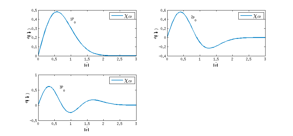
Figure 1: Plots of wave functions for scalar ($0^{++}$) quarkonia $\chi_{c0}$ Vs $\widehat{q}$ (in Gev.) for the states $1P,2P$ and $3P$.

The mass spectrum of ground and excited states for equal mass heavy scalar ($0^{++}$) mesons is written as:

$$\frac{1}{2\beta_{s}^{2}}(\frac{M^{2}}{4}-m^{2}+\frac{C_{0}\beta_{s}^{4}}{\omega^{2}_{0}}\sqrt{1+2A_{0}(N+\frac{3}{2})})=N+\frac{3}{2};N=2n+l;n=0,1,2,...,$$ (18)

where the orbital quantum number, $l=1$. Now, treating the mass spectral equation, Eq.(12) as the unperturbed equation, with the unperturbed wave functions, $\phi_{S}(nP,\widehat{q})$ for scalar mesons in Eq.(17), we now incorporate the OGE (coulomb) term in this equation.

Then the above mass spectral equation can be written as:

$$E_{S}\phi_{S}(\hat{q})=[-\beta_{S}^{4}\overrightarrow{\nabla}^{2}_{\hat{q}}+\hat{q}^{2}+V_{coul}^{S}]\phi_{S}(\hat{q}),$$ (19)

Treating the coulomb term as a perturbation to the unperturbed mass spectral equation, we can write the complete mass spectra for the ground and excited states for equal mass heavy scalar ($0^{++}$) mesons using first order perturbation theory as:

$$\frac{1}{2\beta_{S}^{2}}\{\frac{M^{2}}{4}-m^{2}+\frac{\beta_{S}^{4}C_{0}}{\omega_{0}^{2}}\sqrt{1+2A_{0}(N+\frac{3}{2})}\}+\gamma<V_{coul}^{S}>=(N+\frac{3}{2});N=2n+l;n=0,1,2....,$$ (20)

with $l=1$, where $<V_{coul}^{S}>$ is the expectation value of $V_{coul}^{S}$ between the unperturbed states of given quantum numbers $n$ (with $l=1$) for scalar mesons, and has been weighted by a factor of $\gamma=\frac{C_{0}^{2}\beta_{S}^{4}}{(m_{1}+m_{2})^{2}}$ to have the coulomb term dimensionally consistent with the harmonic term. Its expectation values for the $1P,2P$, and $3P$ states are:

$$<1P|V_{coul}^{S}|1P>=-\frac{128\pi\alpha_{s}}{9\beta_{S}^{2}},$$

$$<2P|V_{coul}^{S}|2P>=-\frac{64\pi\alpha_{s}}{18\beta_{S}^{2}},$$

$$<3P|V_{coul}^{S}|3P>=-\frac{3712\pi\alpha_{s}}{213\beta_{S}^{2}}$$ (21)

	BSE-CIA	Expt [6]	Pot.Model[27]	BSE[20]	RQM[28]
$M_{\chi c0}(1p_{0})$	3.4186	3.4140$\pm$0.0003	3.440		3.413
$M_{\chi c0}(2p_{0})$	4.1804		3.9200	3.8368	3.8700
$M_{\chi c0}(3p_{0})$	5.0323			4.1401	4.3010

Table 2: Mass spectrum of ground and excited states of $\chi_{c0}$ with quantum numbers $J^{PC}=0^{++}$ in GeV. units with the above set of parameters.

From the mass spectral equation, one can see that, the mass spectra depends not only on the principal quantum number $N$, but also the orbital quantum number $l$. We are now in a position to calculate the numerical values for mass spectral of heavy equal mass scalar meson with the input parameters of our model. The results of mass spectral predictions of heavy equal mass scalar mesons for both ground and excited states with the above set of parameters is given in table 2.

We now derive the mass spectral equations with the incorporation of the OGE (Coulomb) term for pseudoscalar and vector quarkonia, and obtain their solutions in the next section (the preliminary calculations using only the confining part of interaction were done in [30]).

3 Mass spectral equation for pseudoscalar ($0^{-+}$), and vector ($1^{--}$) quarkonia

For pseudoscalar (P), and vector (V) quarkonia, the general decomposition of instantaneous BS wave function of dimensionality $M$ in the center of mass frame is given in Eqs. (18), and (25) respectively in [30]. Putting this wave function in Eqs.(18)(for P-mesons), or Eq.(25) (for V-mesons) into the Salpeter equations leads to two coupled equations in leading amplitudes ($\phi_{1}$, and $\phi_{2}$) for P-mesons, and ($\chi_{1}$, and $\chi_{2}$) for V-mesons. Decoupling them in the heavy-quark limit, leads to Eqs.(37) (for both P and V-mesons) of [30] given as,

$$E_{P,V}\phi_{s}=[-\beta_{P,V}^{4}\overrightarrow{\nabla}_{\widehat{q}}^{2}+\widehat{q}^{2}]\phi_{P,V}(\widehat{q}),$$ (22)

with non-perturbative energy eigen functions for $l=0(S)$, and for $l=2(D)$ states obtained as solutions of above spectral equation in approximate harmonic oscillator basis for pseudoscalar quarkonia (for states $1S,...,4S$) and vector quarkonia (for states $1S,...,3D$) as Eq.(41) in [30], for the perturbative calculation of the short ranged one-gluon-exchange interaction shown later in this section.

The plots of unperturbed wave functions for pseudoscalar and vector quarkonia are given in [30]. The unperturbed mass spectra is expressed as (see[30]),

$$[\frac{M^{2}}{4}-m^{2}+\frac{\beta_{P,V}^{4}C_{0}}{\omega_{0}^{2}}\sqrt{1+2A_{0}(N+3/2)}]=2\beta_{P,V}^{2}(N+\frac{3}{2});N=2n+l;n=0,1,2,...$$ (23)

The mass spectra of vector charmonium and bottomonium states using the above spectral equation was found to have degenerate $S$, and $D$ states [30]. However with the incorporation of the OGE (Coulomb) term the mass spectral equation can be written as:

$$E_{P,V}\phi_{P,V}(\hat{q})=[-\beta_{P,V}^{4}\overrightarrow{\nabla}^{2}_{\hat{q}}+\hat{q}^{2}+V_{coul}^{P,V}]\phi_{P,V}(\hat{q}),$$ (24)

Now, treating the coulomb term as a perturbation to the unperturbed mass spectral equation, Eq.(22), and treating the wave functions $\phi_{P,V}(\widehat{q})$ in Eq.(41) of [30], as the unperturbed wave functions, we can write the complete mass spectra of ground (1S) and excited states for equal mass heavy pseudoscalar ($0^{-+}$) and vector ($1^{--}$) mesons respectively using the first order degenerate perturbation theory as:

$$\frac{1}{2\beta_{P,V}^{2}}\{\frac{M^{2}}{4}-m^{2}+\frac{\beta_{P,V}^{4}C_{0}}{\omega_{0}^{2}}\sqrt{1+2A_{0}(N+\frac{3}{2})}\}+\gamma<V_{coul}^{P,V}>=(N+\frac{3}{2});N=2n+l;n=0,1,2....,$$ (25)

where $<V_{coul}^{P,V}>$ (has again been weighted by a factor of $\gamma_{P,V}=\frac{C_{0}^{2}\beta_{P,V}^{4}}{(m_{1}+m_{2})^{2}}$, as in scalar ($0^{++}$) quarkonia in previous section) is the matrix element of $V_{coul}^{P,V}$ between unperturbed states in Eq.(41) of [30] of given quantum numbers $n$, and $l$, (with $n=0,1,2,3,...$, and $l=0$ for pseudoscalar mesons, while with $l=0,2$ for vector mesons). It is to be noted that, $V_{coul}^{P,V}$ connects only the equal parity states with the same values of quantum numbers $n$. The only non-vanishing matrix elements of the perturbation between states with the given quantum numbers $n$ and $l$ are listed below:

$$<nS|V_{coul}^{P}|nS>=\frac{\pi\alpha_{s}}{12}\frac{1}{\beta_{P}^{2}}$$

$$<nS|V_{coul}^{V}|nS>=\frac{\pi\alpha_{s}}{24}\frac{1}{\beta_{V}^{2}}$$

$$<nD|V_{coul}^{V}|nD>=\frac{\pi\alpha_{s}}{24}\frac{1}{5\beta_{V}^{2}},$$ (26)

The non-zero values of $<V_{coul}>$ given above not only lead to the lifting up of the degeneracy between the $S$ and $D$ levels with the same principal quantum number $N$ in vector quarkonia, but also leads to bringing the masses of different states of vector and pseudoscalar quarkonia closer to data, as can be seen from the mass spectral results for pseodoscalar ($0^{-+}$), and vector ($1^{--}$) quarkonia, which are compared with the experimental data [6], and other models for each state (where ever available), as given in Tables 3 and 4 respectively as:

	BSE - CIA	Expt.[6]	Pot. Model[40]	QCD sum rule[15]	Lattice QCD[12]	[28]
$M_{\eta_{c}(1S)}$	2.9822	2.983$\pm$0.0007	2.980	3.11$\pm$0.52	3.292	2.981
$M_{\eta_{c}(2S)}$	3.7395	3.639$\pm$0.0013	3.600		4.240	3.635
$M_{\eta_{c}(3S)}$	4.4256		4.060			3.989
$M_{\eta_{c}(4S)}$	5.0843		4.4554			4.401

Table 3: Masses of ground and radially excited states of $\eta_{c}$ (in GeV.) in present calculation (BSE-CIA) along with experimental data, and their masses in other models.

	BSE - CIA	Expt.[6]	Rel. Pot. Model[28]	Pot. Model[40]	BSE[20]	Lattice QCD[41]
$M_{J/\psi(1S)}$	3.0897	3.0969$\pm$ 0.000011	3.096	3.0969		3.099
$M_{\psi(2S)}$	3.7004	3.6861$\pm$ 0.00034	3.685	3.6890	3.686	3.653
$M_{\psi(1D)}$	3.7878	3.773$\pm$ 0.00033	3.783		3.759
$M_{\psi(3S)}$	4.278	4.03$\pm$ 0.001	4.039	4.1407	4.065	4.099
$M_{\psi(2D)}$	4.3444	4.191$\pm$0.005	4.150		4.108
$M_{\psi(4S)}$	4.8035	4.421$\pm$0.004	4.427	4.5320	4.344
$M_{\psi(3D)}$	4.8617		4.507		4.371
$M_{\psi(5S)}$	5.1391		4.837	4.8841	4.567
$M_{\psi(4D)}$	5.1449		4.857

Table 4: Masses of ground, radially and orbitally excited states of heavy vector quarkonium, $J/\psi$ in BSE-CIA along with their masses in other models and experimental data (all units are in GeV).

4 Mass spectral equation for axial vector $1^{++}$ quarkonia

The general form for the relativistic Salpeter wave function of ${}^{3}P_{1}$ state with $J^{PC}=1^{++}$ can be expressed as in [17, 19]. In the center of mass frame, we can then write the general decomposition of the instantaneous BS wave function for axial vector mesons $(J^{pc}=1^{++})$ of dimensionality $M$ as:

$$\psi(\hat{q})=\gamma_{5}[\gamma_{\mu}+\frac{P_{\mu}\not{P}}{M^{2}}][iMg_{1}(\hat{q})+\not{P}g_{2}(\hat{q})-\not{\hat{q}}g_{3}(\hat{q})+2i\frac{\not{P}\not{\hat{q}}}{M}g_{4}(\hat{q})]$$

$$+\gamma_{5}[M\hat{q_{\mu}}g_{3}(\hat{q})+2i\hat{q_{\mu}}\not{P}g_{4}(\hat{q})].$$ (27)

With use of our power counting rule [23, 24], it can be checked that the Dirac structures associated with amplitudes $g_{1}$ and $g_{2}$ are $O(M^{1})$, and are leading, and would contribute maximum to any axial vector meson calculation. Following a similar procedure as in the case of scalar mesons, we can write the Salpeter wave function in terms of only two leading Dirac amplitudes $g_{1}$, and $g_{2}$. Plugging this wave function together with the projection operators into the first two Salpeter equations in Eq.(16) of [30], and taking trace on both sides and following the steps as for the scalar meson case, we get the coupled integral equations in the amplitudes $g_{1}$, and $g_{2}$:

$$(M-2\omega)[-\frac{2mg_{1}}{\omega}+2g_{2}]=\Theta_{A}\int\frac{d^{3}\widehat{q}^{\prime}}{(2\pi)^{3}}V_{c}(\widehat{q},\widehat{q}^{\prime})[-\frac{2mg_{1}}{\omega}+2g_{2}],$$

$$(M-2\omega)[-\frac{2mg_{1}}{\omega}+2g_{2}]=-\Theta_{A}\int\frac{d^{3}\widehat{q}^{\prime}}{(2\pi)^{3}}V_{c}(\widehat{q},\widehat{q}^{\prime})[-\frac{2mg_{1}}{\omega}+2g_{2}].$$ (28)

To decouple these equations, we follow a similar procedure as in the scalar meson case, and get two identical decoupled equations, one entirely in $g_{1}(\hat{q})$, and the other that is entirely in, $g_{2}(\hat{q})$. In the limit, $\omega\approx m$ on RHS, and due to the fact that for axial quarkonia again, $\omega_{q\bar{q}}^{4}\ll\omega_{q\bar{q}}^{2}$ these equations can be expressed as:

$$[\frac{M^{2}}{4}-m^{2}-\hat{q}^{2}]g_{1}(\hat{q})=-m\Theta_{A}\omega_{q\bar{q}}^{2}[\vec{\nabla}_{\hat{q}}^{2}+\frac{C_{0}}{\omega_{0}^{2}}]g_{1}(\hat{q})$$

$$[\frac{M^{2}}{4}-m^{2}-\hat{q}^{2}]g_{2}(\hat{q})=-m\Theta_{A}\omega_{q\bar{q}}^{2}[\vec{\nabla}_{\hat{q}}^{2}+\frac{C_{0}}{\omega_{0}^{2}}]g_{2}(\hat{q})$$ (29)

where, it can be checked that both $g_{1}$ and $g_{2}$ satisfy the same equation and hence we can approximately write $g_{1}\sim g_{2}\sim\phi_{A}$. Thus,

$$[\frac{M^{2}}{4}-m^{2}-\hat{q}^{2}]\phi_{A}(\hat{q})=-\Theta_{A}m\omega_{q\bar{q}}^{2}[\vec{\nabla}_{\hat{q}}^{2}+\frac{C_{0}}{\omega_{0}^{2}}]\phi_{A}(\hat{q}),$$ (30)

where $\Theta_{A}=\gamma_{\mu}\Psi(\widehat{q})\gamma_{\mu}$. Now, with the use of leading Dirac structures, we can again to a good approximation express $\Theta_{A}=2$. This is due to the fact that $\gamma_{\mu}\psi(\widehat{q})\gamma_{\mu}\approx\gamma_{\mu}\gamma_{5}\gamma_{\nu}(iMg_{1})\gamma_{\mu}=2\gamma_{5}\gamma_{\nu}(iMg_{1})\approx 2\psi(\widehat{q})$. This mass spectral equation has the same form as the mass spectral equation for scalar quarkonia, Eq. (10), except for the value of $\Theta_{A}$, which is different from $\Theta_{S}$. Thus the above equation can be put in a similar form as Eq.(12) (for scalar case), except that inverse range parameter $\beta_{s}\rightarrow\beta_{A}$, where, $\beta_{A}=(\frac{2m\omega_{q\bar{q}}^{2}}{\sqrt{1+2A_{0}(N+3/2)}})^{1/4}$, and the $3D$ wave function, $\phi_{s}\rightarrow\phi_{A}$. The mass spectral equation for $1^{++}$ would then exactly resemble Eqs.(18) for $0^{++}$ case, and thus the unperturbed wave functions $\phi_{A}(\widehat{q})$ for $1^{++}$ would then have the same algebraic form as $\phi_{s}(\widehat{q})$ in Eqs.(17), but with $\beta_{s}\rightarrow\beta_{A}$:

$$\phi_{A}(1p,\hat{q})=(\frac{2}{3})^{1/2}\frac{1}{\pi^{3/4}\beta_{A}^{5/2}}\hat{q}e^{-\frac{\hat{q}^{2}}{2\beta_{A}^{2}}},$$

$$\phi_{A}(2p,\hat{q})=(\frac{5}{3})^{1/2}\frac{1}{\pi^{3/4}\beta_{A}^{5/2}}\hat{q}\bigg{[}1-\frac{2}{5}\frac{\hat{q}^{2}}{\beta_{A}^{2}}\bigg{]}e^{-\frac{\hat{q}^{2}}{2\beta_{A}^{2}}},$$

$$\phi_{A}(3p,\hat{q})=(\frac{70}{171})^{1/2}\frac{1}{\pi^{3/4}\beta_{A}^{5/2}}\hat{q}\bigg{[}1-\frac{2\hat{q}^{2}}{5\beta_{A}^{4}}+\frac{4\hat{q}^{4}}{35\beta_{A}^{4}}\bigg{]}e^{-\frac{\hat{q}^{2}}{2\beta_{A}^{2}}}$$ (31)

The plots of wave functions for axial vector quarkonia are given in Fig.2 below

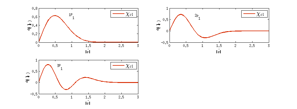
Figure 2: Plots of wave functions for axial vector ($1^{++}$) quarkonia $\chi_{c1}$ Vs $\widehat{q}$ (in Gev.) for the states $1P,2P$ and $3P$.

Now, the perturbative inclusion of the coulomb term will reduce mass spectrum for axial vector meson in the same form as Eqs.(19) -(21) for the scalar case, except that the inverse range parameter $\beta_{s}$ has got to be replaced by $\beta_{A}$. This complete mass spectral equation for ground and excited states of $1^{++}$ is:

$$E_{A}\phi_{A}(\hat{q})=[-\beta_{A}^{4}\overrightarrow{\nabla}^{2}_{\hat{q}}+\hat{q}^{2}+V_{coul}^{A}]\phi_{A}(\hat{q}),$$ (32)

The solutions of the above spectral equation is:

$$\frac{1}{2\beta_{A}^{2}}\{\frac{M^{2}}{4}-m^{2}+\frac{\beta_{A}^{4}C_{0}}{\omega_{0}^{2}}\sqrt{1+2A_{0}(N+\frac{3}{2})}\}+\gamma_{A}<V_{coul}^{A}>=(N+\frac{3}{2});N=2n+l;n=0,1,2....,$$ (33)

with $l=1$, where $<V_{coul}^{A}>$ is the expectation value of $V_{coul}^{A}$ between the unperturbed states of given quantum numbers $n$ (with $l=1$) for axial vector mesons, and has been weighted by a factor of $\gamma_{A}=\frac{C_{0}^{2}\beta_{A}^{4}}{(m_{1}+m_{2})^{2}}$ to have the coulomb term dimensionally consistent with the harmonic term. Its expectation values for the $1P,2P$, and $3P$ states are:

$$<1P|V_{coul}^{A}|1P>=-\frac{64\pi\alpha_{s}}{9\beta_{A}^{2}},$$

$$<2P|V_{coul}^{A}|2P>=-\frac{32\pi\alpha_{s}}{18\beta_{A}^{2}},$$

$$<3P|V_{coul}^{A}|3P>=-\frac{1856\pi\alpha_{s}}{213\beta_{A}^{2}}$$ (34)

From the mass spectral equation, one can see that, the mass spectra again depends not only on the principal quantum number $N$, but also the orbital quantum number $l$. We are now in a position to calculate the numerical values for mass spectra of heavy scalar quarkonia with the input parameters of our model as mentioned above. The results of mass spectral predictions of heavy equal mass scalar mesons for both ground and excited states with the above set of parameters is given in table 2. The results on masses of ground ($1P$) and excited ($2P$ and $3P$) states of quarkonia, $\chi_{c1}$ are given in Table 5.

	BSE-CIA	Expt [6]	Pot.Model[27]	BSE[20]	RQM[28]
$M_{\chi c1}(1p_{1})$	3.5128	3.510$\pm$0.0007	3.440		3.413
$M_{\chi c1}(2p_{1})$	3.9398	3.871.69$\pm$0.0017	3.920	3.928	3.870
$M_{\chi c1}(3p_{1})$	4.4616			4.228	4.301

Table 5: Mass spectrum of ground and excited states of $\chi_{c1}$ with quantum numbers $J^{PC}=1^{++}$ in GeV. units with the above set of parameters.

5 Two-photon decays of scalar quarkonium

We now study the two-photon decay width of a scalar quarkonium ($0^{++}$), which proceeds through the quark-triangle diagrams shown in Fig.3.

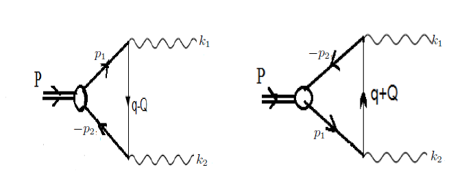
Figure 3: Diagrams contributing to the two-photon decays of scalar ($0^{++}$) quarkonia

Let $P$ be the total momentum of the scalar quarkonia, and $k_{1.2}$ be the momenta of the two emitted photons with polarizations $\varepsilon_{1,2}$ respectively. Then we can write $P=k_{1}+k_{2}$, and let $2Q=k_{1}-k_{2}$. The invariant amplitude for this process can be written as:

$$M_{fi}(S\rightarrow\gamma\gamma)=\frac{i\sqrt{3}(ie_{Q})^{2}}{m^{2}+\frac{M^{2}}{4}}\int\frac{d^{3}\widehat{q}}{(2\pi)^{3}}Tr[\Psi^{s}(\widehat{q})[\not{\epsilon_{1}}(m+i\not{Q})\not{\epsilon_{2}}+\not{\epsilon_{2}}(m+i\not{Q})\not{\epsilon_{1}}]].$$ (35)

where $e_{Q}=+\frac{2}{3}e$ for $c\overline{c}$, The 3D structure of Dirac wave function, $\Psi^{s}(\widehat{q})$ is given in Eqs.(9), and (17). The propagators for the third quark in the two diagrams is expressed as, $S_{F}(q\mp Q)=\frac{-i(\not{q}\mp\not{Q})+m}{(q\mp Q)^{2}+m^{2}}$. Now for heavy hadrons, where the system can be regarded as non-relativistic, it is a good approximation to take the internal momentum $q<<M$, and hence $q^{2}<<Q^{2}$, where it can be seen that $Q^{2}=\frac{M^{2}}{4}$. Using the propagator expressions given above, and evaluating trace over the gamma matrices, we can write the invariant amplitude given above as:

$$M_{fi}(S\rightarrow\gamma\gamma)=(\epsilon_{1}.\epsilon_{2})F_{S},$$

$$F_{S}=(\frac{16\alpha_{em}}{3\sqrt{3}\pi^{2}})\frac{mM}{m^{2}+\frac{M^{2}}{4}}\int d^{3}\widehat{q}\phi_{s}(\widehat{q})$$ (36)

where $F_{S}$ is the decay constant for scalar quarkonium, $\chi_{c0}$. The decay width for the process can then be expressed as,

$$\Gamma(S\rightarrow\gamma\gamma)=\frac{1}{32\pi M}|F_{S}|^{2}.$$ (37)

	BSE-CIA	Expt [6]	Pot.Model[27]	BSE[42]	RQM[43]
$\Gamma_{\chi_{c0}(1p_{1})\rightarrow\gamma\gamma}$	2768.05	2341.50	1290.00$\pm$3.45	1390.00	2900.00
$\Gamma_{\chi_{c0}(2p_{1})\rightarrow\gamma\gamma}$	1548.20		950.00$\pm$3.88	1110.00$\pm$130.00	1900.00

Table 6: Two-photon decay widths of ground and first excited states of $\chi_{c0}(1P)$ and $\chi_{c0}(2P)$ in eV with the input set of parameters given after Eq.(7)

6 Discussions

We have employed a 3D reduction of BSE (with a $4\times 4$ representation for two-body ($q\overline{q}$) BS amplitude) under Covariant Instantaneous Ansatz (CIA) for deriving the algebraic forms of the mass spectral equations for scalar, pseudoscalar, vector and axial vector quarkonia using the full BS kernel comprising of the one-gluon-exchange and the confining part in an approximate harmonic oscillator basis that led to analytic solutions (both eigen functions and eigen values). We thus obtain the mass spectra of $c\overline{c}$ quarkonia for ground and excited states of $0^{++}$, $0^{-+}$ , $1^{--}$,and $1^{++}$ states. The mass spectral results for all these states which are compared with the experimental data [6], and other models for each state (where ever available), are given in Tables 2-5 respectively. The masses, and the algebraic forms of eigen functions for each quarkonium state so obtained will be used for calculating their various transitions.

Here we wish to mention that in principle, in $Q\overline{Q}$ quarkonia, the constituents are close enough to each other to warrant a more accurate treatment of the coulomb term. Though for $b\overline{b}$ systems, the coulomb term will be extremely dominant in comparison to confining term, however, it may not be so unreasonable to treat coulomb term perturbatively for $c\overline{c}$ systems. Here, we wish to point out that if we are getting reasonable results for orbital $c\overline{c}$ excitations, it is mainly due to centrifugal effects[34] which ensure that $c-\overline{c}$ separation is large enough to feel the effect of confining term more strongly than the coulomb term. Further, the present approach is on lines of some earlier works [34, 35, 36] where the OGE(coulomb) term is treated perturbatively for charmed mesons and baryons. Similarly in a recent work [37], the 3D harmonic oscillator wave functions were used as a trial wave functions for obtaining $c\overline{c}$ spectrum and their decays, where these trial wave functions did not take into account the importance of coulomb potential for heavy quarkonium systems. Similar treatment was earlier followed in [38].

Also, in our recent work [30] in which one of us (SB) was involved, we did not take into account the coulomb interactions between $c\overline{c}$, and $b\overline{b}$ states, and used only the confining interaction to study their spectra and decays on lines of other works [31, 32, 33].

However, in the present approach, using confining interactions alone, we first analytically derive the algebraic forms of wave functions for various $c\overline{c}$ states, which are of harmonic oscillator form. Though we then introduce coulomb term perturbatively for $c\overline{c}$, (and not for $b\overline{b}$), this present calculation is a substantial improvement over our previous work in [30] (where we did not treat coulomb interaction at all). However, for $b\overline{b}$ states, a more exact non-perturbative treatment of coulomb interaction would be needed.

Further, our results on $c\overline{c}$ mass spectra suggest that perturbative incorporation of OGE with use of harmonic oscillator wave functions derived analytically is closer to reality than some of the previous approaches[37, 38] where they used h.o. wave functions only as trial wave functions which did not take into account the importance of coulomb potential for heavy quarkonium systems.

All numerical calculations have been done using Mathematica. We selected the best set of 6 input parameters (given after Eq.(11)), that gave good matching with data for masses of ground and excited states of $c\overline{c}$, and $b\overline{b}$ quarkonia for pseudoscalar and vector states. The same set of parameters above was also used to calculate the leptonic decay constants of $\eta_{c},\eta_{b},J/\psi$, and $\Upsilon$, as well as the two-photon and two-gluon decay widths of $\eta_{c}$, and $\eta_{b}$ in [30], which were in in reasonable agreement with experiment and other models.

Using the same set of input parameters, we have predicted the full mass spectrum of ground ($1P$), and excited ($2P$ and $3P$) states of $\chi_{c0}$ and $\chi_{c1}$. Also we calculated the full spectrum of $1S,...,4S$ states of $\eta_{c}$, as well as $1S,...,4D$ states of $J/\Psi$. The analytic forms of wave functions derived for $0^{++}$ states of $c\overline{c}$ were employed to calculate their two-photon decays .

We wish to also point out that the present calculation with perturbative incorporation of the one-gluon-exchange interaction, also lifts up the degeneracy between the $S$ and $D$ states of vector quarkonia, and also giving a better agreement with the data for these states. The results obtained for the ground ($1P$) state of $\chi_{c0}$, as well as the ground and first excited states of $\chi_{c1}$ are in reasonable agreement with data. However, there are open questions about the quantum number assignments of the state $X(3915)$, which is available in PDG tables. Some authors [7, 8] argue that it is difficult to assign $X(3915)$ to $\chi_{c0}(2P)$, and that it could be $\chi_{c2}(2P)$. The possible mass of $\chi_{c0}(2P)$ was recently predicted by [7] as $3.837\pm 0.0115$ MeV. We then worked out the decay widths of $\chi_{c0}$ for ground (1P), and excited (2P) states, and compared our results with data and other models in Table 6. We further calculated the two photon decay widths of $\chi_{c0}$ for $1P$, and $2P$ states. Though our results are smaller than data [6], but compares well with other models [27, 42]. Further a large variation in decay widths can be seen in other models.

We further wish to point out that this analytic approach (giving explicit dependence of spectra on principal quantum number $N$) under heavy quark approximation gives a much deeper insight into the spectral problem, than the purely numerical approaches prevalent in the literature. The plots of the analytical forms of wave functions for various $J^{PC}$ states, obtained as solutions of their mass spectral equations are also are given in Figs.1- 2 for scalar and axial vector quarkonia. The correctness of our approach can be gauged by the fact that these plots are very similar to the corresponding plots of amplitudes for these quarkonia in [20] obtained by purely numerical methods. The analytical forms of eigen functions for ground and excited states so obtained can be used to evaluate the various other processes involving scalar and axial vector quarkonia, which we intend to do next.

Acknowledgements: This work was carried out at Addis Ababa University, Ethiopia, and at Chandigarh University, India. The authors wish to thank both the institutions for the facilities provided during the course of this work. One of us (LA) wishes to thank Samara University, Ethiopia for support for his Doctoral programme. He also wishes to thank Chandigarh University for the hospitality during his visit during August-October 2017.

99

References

- [1] N.Brambilla, A.Pineda, J.Soto, A.Vairo, Rev. Mod. Phys. 77, 1423 (2005).
- [2] K. M. Ecklund et al. (CLEO Collaboration), Phys. Rev. D 78, 091501 (2008).
- [3] B.Auger et al.(BaBar collaboration), Phys. Rev. Lett. 103, 161801 (2009).
- [4] K.F.Chen et al.(Belle collaboration), Phys. Rev. D82, 091106(R) (2010).
- [5] K.W.Edwards et al.(CLEO collaboration), Phys. Rev.Lett. 86, 30 (2001).
- [6] K.A.Olive et al., (Particle Data Group), Chin. Phys. C38, 090001 (2014).
- [7] F.K.Guo, U-G. Meisner, Phys. Rev. D86, 091501 (2012).
- [8] S.L.Olsen, Phys. Rev. D91, 057501 (2015).
- [9] N.Brambilla et al., Eur. Phys, J. C71, 1534 (2011).
- [10] C.McNielle, C.T.H.Davies, E.Follana, K.Hornbostel, G.P.Lepage (HPQCD Collaboration), arxiv: 1207.0994[hep-lat] (2012).
- [11] G.S.Bali, K.Schiling, and A. Wachter, Phys Rev. D 56, 2566 (1997).
- [12] T.Burch et al.(Fermilab and MILC Collaboration), Phys. Rev. D81, 034508 (2010).
- [13] J.Gasser, H.Leutwyler, Ann. Phys. 158, 142 (1984).
- [14] M.A.Shifman, A.I.Vainshtein, V.I.Zakharov, Nucl. Phys. B147, 385, 448 (1979).
- [15] E.Veli Veliev, K.Azizi, H.Sundu, N.Aksit, J.Phys. G39, 015002(2012).
- [16] G.T.Bodwin, E.Braaten, G.P.Lepage, Phys. Rev. D51, 1125 (1995).
- [17] C.H.L.Smith, Ann. Phys. (N.Y.) 53, 521 (1969).
- [18] A. N. Mitra, B. M. Sodermark, Nucl. Phys. A695, 328 (2001).
- [19] R. Alkofer, L. W. Smekel, Phys. Rep.353, 281 (2001).
- [20] C-H. Chang, G. L. Wang, Sci. China G53, 2005 (2010).
- [21] A.N.Mitra, S.Bhatnagar, Intl. J. Mod. Phys. A07, 121 (1992).
- [22] S.Bhatnagar, D.S.Kulshreshtha, A.N.Mitra, Physics Letters B 263, 485 (1991).
- [23] S. Bhatnagar, S-Y. Li, J. Phys. G32, 949 (2006)
- [24] S. Bhatnagar, S-Y.Li, J. Mahecha, Int. J. Mod. Phys. E20, 1437 (2011).
- [25] S.Bhatnagar, J.Mahecha, Y.Mengesha, Phys. Rev. D90, 014034 (2014).
- [26] H.Negash, S.Bhatnagar, Advances in High Energy Physics 2017, 7306825 (2017).
- [27] S.Godfrey, N. Isgur, Phys. Rev. D32, 189 (1985).
- [28] D.Ebert, R.N.Faustov, V.O.Galkin, Phys. Atomic Nuclei 76, 1554 (2013); arXv:1111 .0454v1[hep-ph] (2011).
- [29] S.Patel, P.C.Vinodkumar, S.Bhatnagar, Chinese Physics C40, 053102 (2016).
- [30] H. Negash and S.Bhatnagar, Intl. J. Mod. Phys. E25, 1650059 (2016).
- [31] R. Ricken, M. Koll, D. Merten, B. Metsch, H. Petry, Eur. Phys. J. A9, 221 (2000).
- [32] T.Babutsidze, T.Kopaleishvili, A. Rusetsky, Phys. Rev. C59, 976 (1999).
- [33] M. G. Olsson, A. D. Martin, and A.W. Peacock, Phys. Rev. D 31,81 (1985).
- [34] A.N.Mitra, I. Santhanam, Z. phys. C8, 33 (1981).
- [35] A.Majethiya, B.Patel, A.K.Rai, P.C.Vinodkumar, arxiv 0809.4910[hep-ph].
- [36] F.Arleo, J.Cugnon, Y.Kalinovsky, Phys. Lett. B614, 44 (2005).
- [37] Bhaghyesh, K.B. Vijayakumar, Chin. Phys. C37, 023103 (2013).
- [38] S.Capstick, S.Godfrey, Phys. Rev. D41, 2856 (1990).
- [39] S.Bhatnagar, M.Li, S-Y.Li, J. Mod. Phys.5, 1027 (2014).
- [40] Bhagyesh, K.B.V.Kumar, A.P.Monterio, J.Phys. G38, 085001 (2011).
- [41] T.Kawanai, S.Sasaki, arxiv:1503.05752[hep-lat].
- [42] C.R.Munz, arxiv: hep-ph/9601206
- [43] D.Ebert, R.N.Faustov, V.O.Galkin, arxiv: hep-ph/0302044.
99