Shallow water equations: Split-form, entropy stable, well-balanced, and positivity preserving numerical methods

Abstract

For the first time, a general two-parameter family of entropy conservative numerical fluxes for the shallow water equations is developed and investigated. These are adapted to a varying bottom topography in a well-balanced way, i.e. preserving the lake-at-rest steady state. Furthermore, these fluxes are used to create entropy stable and well-balanced split-form semidiscretisations based on general summation-by-parts (SBP) operators, including Gauß nodes. Moreover, positivity preservation is ensured using the framework of Zhang and Shu (Maximum-principle-satisfying and positivity-preserving high-order schemes for conservation laws: survey and recent developments, 2011. In: Proceedings of the Royal Society of London A: Mathematical, Physical and Engineering Sciences, The Royal Society, vol 467, pp. 2752–2766). Therefore, the new two-parameter family of entropy conservative fluxes is enhanced by dissipation operators and investigated with respect to positivity preservation. Additionally, some known entropy stable and positive numerical fluxes are compared. Furthermore, finite volume subcells adapted to nodal SBP bases with diagonal mass matrix are used. Finally, numerical tests of the proposed schemes are performed and some conclusions are presented.

1 Introduction

For the first time, a two-parameter family of entropy conservative and well-balanced numerical fluxes for the shallow water equations is investigated, resulting in genuinely high-order semidiscretisations that are both entropy stable and positivity preserving. These semidiscretisations of the shallow water equations in one space dimension are based on summation-by-parts (SBP) operators, see inter alia the review articles by Svärd and Nordström (2014); Fernández et al (2014) and references cited therein. This setting of SBP operators originates in the finite difference (FD) setting, but can also be used in polynomial methods as nodal discontinuous Galerkin (DG) (Gassner, 2013) or flux reconstruction / correction procedure via reconstruction (Ranocha et al, 2016).

Entropy stability has long been known as a desirable stability property for conservation laws. Here, the semidiscrete setting of Tadmor (1987, 2003) will be used. Other desirable stability properties for the shallow water equations are the preservation of non-negativity of the water height and the correct handling of steady states, especially the lake-at-rest initial condition, resulting in well-balanced methods.

References for numerical methods for the shallow water equations can be found in the review article of Xing and Shu (2014) and references cited therein.

This article extends the entropy conservative split form of Gassner et al (2016b); Wintermeyer et al (2016) to a new two-parameter family of well-balanced and entropy conservative splittings. Moreover, SBP bases not including boundary nodes are considered and corresponding semidiscretisations are developed in one spatial dimension. To the author’s knowledge, this general two-parameter family of numerical fluxes has not appeared in the literature before.

Furthermore, positivity preservation in the framework of Zhang and Shu (2011) is considered. Therefore, the new fluxes are investigated regarding positivity and finite volume (FV) subcells are introduced. Additionally, some known entropy stable and positivity preserving numerical fluxes are compared.

The extension to general SBP bases can be seen as some kind of ’positive negative result’: It is possible to get the desired properties of the schemes using Gauß nodes, including a higher accuracy compared to Lobatto nodes, but this comes at the cost of complicated correction terms. Therefore, although a similar extension to two-dimensional unstructured and curvilinear grids can be conjectured to exist, it is expected to be even more complex and thus not suited for high-performance production codes.

However, the combination of entropy stability and positivity preservation for the shallow water equations using high-order SBP methods has not been considered before. The results can be expected to be extendable to high-performance codes using Lobatto nodes and the flux-differencing form of Fisher and Carpenter (2013) on two-dimensional unstructured and curvilinear grids if tensor product bases on quadrilaterals are used.

At first, some analytical properties of the shallow water equations are reviewed in section 2 and the existing split form of Gassner et al (2016b); Wintermeyer et al (2016) is described in section 3. Afterwards, a new two-parameter family of entropy conservative numerical fluxes for the shallow water equations with constant bottom topography is developed in section 4 and extended to a varying bottom in section 5. The corresponding semidiscretisation using general SBP bases is designed in section 6. The positivity preserving framework of Zhang and Shu (2011) is introduced to this setting and numerical fluxes based on the entropy conserving schemes are investigated with respect to positivity preservation in section 7. Additionally, some known fluxes are presented. An extension of the idea to use FV subcells to the setting of nodal SBP bases with diagonal mass matrix is proposed in section 8 and numerical experiments are presented in section 9. Finally, the results are summed up in section 10 and some conclusions and directions of further research are presented.

2 Review of some properties of the shallow water equations

The shallow water equations in one space dimension are

$$\partial_{t}\underbrace{\begin{pmatrix}h\\ hv\end{pmatrix}}_{=u}+\,\partial_{x}\underbrace{\begin{pmatrix}hv\\ hv^{2}+\frac{1}{2}gh^{2}\end{pmatrix}}_{=f(u)}=\underbrace{\begin{pmatrix}0\\ -gh\partial_{x}b\end{pmatrix}}_{=s(u,x)},$$ (1)

where $h$ is the water height, $v$ its speed, $hv$ the discharge, $b$ describes the bottom topography, and $g$ is the gravitational constant. In the following, some well known results that will be used in the remainder of this work are presented.

As described inter alia by Bouchut (2004, Section 3.2), Dafermos (2010, Section 3.3), Fjordholm et al (2011); Wintermeyer et al (2016), the entropy / total energy $U=\frac{1}{2}hv^{2}+\frac{1}{2}gh^{2}+ghb=\frac{1}{2}\frac{u_{2}^{2}}{u_{1}}+\frac{1}{2}gu_{1}^{2}+gu_{1}b$, is strictly convex for positive water heights $h>0$. Thus, in this case, the associated entropy variables

$$w=U^{\prime}(u)=\begin{pmatrix}g(h+b)-\frac{1}{2}v^{2}\\ v\end{pmatrix}$$ (2)

and conserved variables $u$ can be used interchangeably. With the entropy flux

$$F=\frac{1}{2}hv^{3}+gh^{2}v+gbhv,$$ (3)

smooth solutions satisfy $\partial_{t}U+\partial_{x}F=0$, and the entropy inequality $\partial_{t}U+\partial_{x}F\leq 0$ will be used as an additional admissibility criterion for weak solutions.

If the bottom topography $b\equiv 0$ is constant, the entropy variables are

$$w=\begin{pmatrix}gh-\frac{1}{2}v^{2}\\ v\end{pmatrix}.$$ (4)

In this case, the flux expressed in terms of the entropy variables ($b\equiv 0$) is

$$f\left(u(w)\right)= \begin{pmatrix}\frac{w_{1}+\frac{1}{2}w_{2}^{2}}{g}w_{2}\\ \frac{w_{1}+\frac{1}{2}w_{2}^{2}}{g}w_{2}^{2}+\frac{1}{2}g\left(\frac{w_{1}+\frac{1}{2}w_{2}^{2}}{g}\right)^{2}\end{pmatrix}=\frac{1}{g}\begin{pmatrix}w_{1}w_{2}+\frac{1}{2}w_{2}^{3}\\ \frac{1}{2}w_{1}^{2}+\frac{3}{2}w_{1}w_{2}^{2}+\frac{5}{8}w_{2}^{4}\end{pmatrix},$$ (5)

and the flux potential ($b\equiv 0$) is given by

$$\psi= \frac{1}{2g}w_{1}^{2}w_{2}+\frac{1}{2g}w_{1}w_{2}^{3}+\frac{1}{8g}w_{2}^{5}=\frac{1}{2}gh^{2}v,$$ (6)

fulfilling $\psi^{\prime}(w)=f\left(u(w)\right)$. Finally, the entropy Jacobian

$$\partial_{w}u=\left(\partial_{u}w\right)^{-1}=\begin{pmatrix}\frac{1}{g}&\frac{v}{g}\\ \frac{v}{g}&h+\frac{v^{2}}{g}\end{pmatrix},\quad\partial_{u}w=\begin{pmatrix}g+\frac{u_{2}^{2}}{u_{1}^{3}}&-\frac{u_{2}}{u_{1}^{2}}\\ -\frac{u_{2}}{u_{1}^{2}}&\frac{1}{u_{1}}\end{pmatrix}=\begin{pmatrix}g+\frac{v^{2}}{h}&-\frac{v}{h}\\ -\frac{v}{h}&\frac{1}{h}\end{pmatrix},$$ (7)

can be expressed by using a scaling of the eigenvectors in the form proposed by Barth (1999, Theorem 4) as

$$\partial_{w}u=RR^{T},\qquad R=\frac{1}{\sqrt{2g}}\begin{pmatrix}1&1\\ v-\sqrt{gh}&v+\sqrt{gh}\end{pmatrix},$$ (8)

where the columns of $R$ are eigenvectors of the flux Jacobian $f^{\prime}(u)$. This scaling has also been used inter alia by Fjordholm et al (2011, Section 2.3).

3 Review of an existing split-form SBP method

In order to fix some notation, present the general setting and motivate the extensions developed in this work, some existing results will be reviewed.

A general SBP SAT semidiscretisation is obtained by a partition of the domain into disjoint elements. On each element, the solution is represented in some basis, mostly nodal bases. These cells are mapped to a standard element for the following computations. There, the symmetric and positive definite mass matrix $\underline{\underline{M}}\,$ induces a scalar product, approximating the $L_{2}$ scalar product. The derivative is represented by the matrix $\underline{\underline{D}}\,$. Interpolation to the (two point) boundary of the cell (interval) is performed via the restriction operator $\underline{\underline{R}}\,$ and evaluation of the values at the right boundary minus values at the left boundary is conducted by the boundary matrix $\underline{\underline{B}}\,=\operatorname{diag}\left(-1,1\right)$. Together, these operators fulfil the summation-by-parts (SBP) property

$$\underline{\underline{M}}\,\underline{\underline{D}}\,+\underline{\underline{D}}{{}^{T}}\underline{\underline{M}}\,=\underline{\underline{R}}{{}^{T}}\underline{\underline{B}}\,\underline{\underline{R}}\,,$$ (9)

mimicking integration by parts on a discrete level $\int_{\Omega}u(\partial_{x}v)+\int_{\Omega}(\partial_{x}u)v=uv\big{|}_{\partial\Omega}$. Here, the notation of Ranocha et al (2016, 2015) has been used. Then, similar to strong form discontinuous Galerkin methods, the semidiscretisation can be written as the sum of volume terms, surface terms, and numerical fluxes at the boundaries.

Gassner et al (2016b) proposed as semidiscretisation of the shallow water equations (1) with continuous bottom topography $b$ in the setting of a discontinuous Galerkin spectral element method (DGSEM) using Lobatto-Legendre nodes in each element, that can be generalised to diagonal norm SBP operators with nodal bases including boundary nodes. Wintermeyer et al (2016) extended this setting to two space dimensions, curvilinear grids and discontinuous bottom topographies. In one space dimension on a linear grid, this semidiscretisation can be written as

$$\partial_{t}\underline{h}= -\underline{\underline{D}}\,\underline{hv}-\underline{\underline{M}}{{}^{-1}}\underline{\underline{R}}{{}^{T}}\underline{\underline{B}}\,\left(\underline{f}^{\mathrm{num}}_{h}-\underline{\underline{R}}\,\underline{hv}\right),$$ (10)

$$\partial_{t}\underline{hv}= -\frac{1}{2}\left(\underline{\underline{D}}\,\underline{hv^{2}}+\underline{\underline{hv}}\,\underline{\underline{D}}\,\underline{v}+\underline{\underline{v}}\,\underline{\underline{D}}\,\underline{hv}\right)-g\underline{\underline{h}}\,\underline{\underline{D}}\,\underline{h}-g\underline{\underline{h}}\,\underline{\underline{D}}\,\underline{b}$$

$$-\underline{\underline{M}}{{}^{-1}}\underline{\underline{R}}{{}^{T}}\underline{\underline{B}}\,\Big{(}\underline{f}^{\mathrm{num}}_{hv}-\underline{\underline{R}}\,\underline{hv^{2}}-\frac{1}{2}g\underline{\underline{R}}\,\underline{h^{2}}$$

$$\qquad\qquad\qquad+\frac{1}{2}g\!\!\leavevmode\resizebox{0.0pt}{8.3333pt}{ $\{\!\!\{$ }\mkern-6.5muh\mkern-6.5mu\leavevmode\resizebox{0.0pt}{8.3333pt}{ $\}\!\!\}$ }\!\!_{-}\!\!\leavevmode\resizebox{0.0pt}{8.3333pt}{ $[\![$ }\mkern-6.5mub\mkern-6.5mu\leavevmode\resizebox{0.0pt}{8.3333pt}{ $]\!]$ }\!\!_{-}\underline{e}_{0}+\frac{1}{2}g\!\!\leavevmode\resizebox{0.0pt}{8.3333pt}{ $\{\!\!\{$ }\mkern-6.5muh\mkern-6.5mu\leavevmode\resizebox{0.0pt}{8.3333pt}{ $\}\!\!\}$ }\!\!_{+}\!\!\leavevmode\resizebox{0.0pt}{8.3333pt}{ $[\![$ }\mkern-6.5mub\mkern-6.5mu\leavevmode\resizebox{0.0pt}{8.3333pt}{ $]\!]$ }\!\!_{+}\underline{e}_{1}\Big{)},$$

where $\underline{e}_{k}$ is the $k$-th unit vector and for cell $i$

$$\!\!\leavevmode\resizebox{0.0pt}{8.3333pt}{ $\{\!\!\{$ }\mkern-6.5muh\mkern-6.5mu\leavevmode\resizebox{0.0pt}{8.3333pt}{ $\}\!\!\}$ }\!\!_{-} =\frac{h_{i,0}+h_{i-1,p}}{2},\quad \!\!\leavevmode\resizebox{0.0pt}{8.3333pt}{ $\{\!\!\{$ }\mkern-6.5muh\mkern-6.5mu\leavevmode\resizebox{0.0pt}{8.3333pt}{ $\}\!\!\}$ }\!\!_{+} =\frac{h_{i,p}+h_{i+1,0}}{2},$$ (11)

$$\!\!\leavevmode\resizebox{0.0pt}{8.3333pt}{ $[\![$ }\mkern-6.5mub\mkern-6.5mu\leavevmode\resizebox{0.0pt}{8.3333pt}{ $]\!]$ }\!\!_{-} =b_{i,0}-b_{i-1,p},\quad \!\!\leavevmode\resizebox{0.0pt}{8.3333pt}{ $[\![$ }\mkern-6.5mub\mkern-6.5mu\leavevmode\resizebox{0.0pt}{8.3333pt}{ $]\!]$ }\!\!_{+} =b_{i+1,0}-b_{i,p}.$$

Here, $h_{i,0},h_{i,p}$ are the values of $h$ at the first and last node $0,p$ in cell $i$, respectively.

Using

$$f^{\mathrm{num}}_{h}=\!\!\leavevmode\resizebox{0.0pt}{8.3333pt}{ $\{\!\!\{$ }\mkern-6.5muh\mkern-6.5mu\leavevmode\resizebox{0.0pt}{8.3333pt}{ $\}\!\!\}$ }\!\!\!\!\leavevmode\resizebox{0.0pt}{7.5pt}{ $\{\!\!\{$ }\mkern-6.5muv\mkern-6.5mu\leavevmode\resizebox{0.0pt}{7.5pt}{ $\}\!\!\}$ }\!\!,\qquad f^{\mathrm{num}}_{hv}=\!\!\leavevmode\resizebox{0.0pt}{8.3333pt}{ $\{\!\!\{$ }\mkern-6.5muh\mkern-6.5mu\leavevmode\resizebox{0.0pt}{8.3333pt}{ $\}\!\!\}$ }\!\!\!\!\leavevmode\resizebox{0.0pt}{7.5pt}{ $\{\!\!\{$ }\mkern-6.5muv\mkern-6.5mu\leavevmode\resizebox{0.0pt}{7.5pt}{ $\}\!\!\}$ }\!\!^{2}+\frac{1}{2}g\!\!\leavevmode\resizebox{0.0pt}{10.49863pt}{ $\{\!\!\{$ }\mkern-6.5muh^{2}\mkern-6.5mu\leavevmode\resizebox{0.0pt}{10.49863pt}{ $\}\!\!\}$ }\!\!,$$ (12)

as numerical (surface) flux, where $\!\!\leavevmode\resizebox{0.0pt}{7.5pt}{ $\{\!\!\{$ }\mkern-6.5mua\mkern-6.5mu\leavevmode\resizebox{0.0pt}{7.5pt}{ $\}\!\!\}$ }\!\!=\frac{a_{-}+a_{+}}{2}$, the resulting scheme

1. conserves the mass in general and the discharge for a constant bottom topography,

2. conserves the total energy which is used as entropy,

3. handles the lake-at-rest stationary state correctly,

i.e. it is conservative, stable and well-balanced, as proved by Wintermeyer et al (2016, Theorem 1). The split form discretisation has been recast into the flux differencing framework of Fisher et al (2013); Fisher and Carpenter (2013) using the ”translations” provided by Gassner et al (2016a, Lemma 1). The resulting volume fluxes are

$$f^{\mathrm{vol}}_{h}=\!\!\leavevmode\resizebox{0.0pt}{8.3333pt}{ $\{\!\!\{$ }\mkern-6.5muhv\mkern-6.5mu\leavevmode\resizebox{0.0pt}{8.3333pt}{ $\}\!\!\}$ }\!\!,\qquad f^{\mathrm{vol}}_{hv}=\!\!\leavevmode\resizebox{0.0pt}{8.3333pt}{ $\{\!\!\{$ }\mkern-6.5muhv\mkern-6.5mu\leavevmode\resizebox{0.0pt}{8.3333pt}{ $\}\!\!\}$ }\!\!\!\!\leavevmode\resizebox{0.0pt}{7.5pt}{ $\{\!\!\{$ }\mkern-6.5muv\mkern-6.5mu\leavevmode\resizebox{0.0pt}{7.5pt}{ $\}\!\!\}$ }\!\!+g\!\!\leavevmode\resizebox{0.0pt}{8.3333pt}{ $\{\!\!\{$ }\mkern-6.5muh\mkern-6.5mu\leavevmode\resizebox{0.0pt}{8.3333pt}{ $\}\!\!\}$ }\!\!^{2}-\frac{1}{2}g\!\!\leavevmode\resizebox{0.0pt}{10.49863pt}{ $\{\!\!\{$ }\mkern-6.5muh^{2}\mkern-6.5mu\leavevmode\resizebox{0.0pt}{10.49863pt}{ $\}\!\!\}$ }\!\!,$$ (13)

i.e. the volume terms in (10) can be rewritten using the differentiation matrix $\underline{\underline{D}}\,$ as $\sum_{k=0}^{p}2D_{ik}f^{\mathrm{vol}}_{ik}$, where $f^{\mathrm{vol}}_{ik}=f^{\mathrm{vol}}(u_{i},u_{k})$.

The split form in (10) corresponds to the entropy conservative fluxes $f^{\mathrm{vol}}$ (13). $f^{\mathrm{num}}$ (12) corresponds to a splitting, too, but exchanging $f^{\mathrm{num}}$ for $f^{\mathrm{vol}}$ does not yield a well-balanced method. Similarly, exchanging $f^{\mathrm{vol}}$ for $f^{\mathrm{num}}$ as surface flux does not work properly, since the numerical flux and source discretisation have to be coupled properly in order to result in a well-balanced discretisation, as described in section 5.

The remaining parts of this paper are dedicated to the investigation of the following questions

1. Are there other entropy conservative fluxes than $f^{\mathrm{vol}}$, $f^{\mathrm{num}}$ and corresponding split forms? (Section 4)

2. Are there other discretisations of $gh\partial_{x}b$ that can be used to get a well-balanced scheme, respecting the lake-at-rest stationary state? (Section 5)

3. Can the split forms be used for a nodal SBP method without boundary nodes, e.g. for Gauß nodes? (Section 6)

4. Are there entropy conservative / stable and positivity preserving numerical fluxes that can be used to apply the bound preserving framework of Zhang and Shu (2011)? If so, is the resulting method still entropy stable and well-balanced? (Section 7)

4 Entropy conservative fluxes and split forms for vanishing bottom topography $b\equiv 0$

In this section, several numerical fluxes and associated split forms of the shallow water equations (1) with constant bottom topography $b\equiv 0$ will be considered.

The numerical flux $f^{\mathrm{num}}(u_{-},u_{+})$ has to be consistent, i.e. $f^{\mathrm{num}}(u,u)=f(u)$. In order to be entropy conservative, the condition

$$\!\!\leavevmode\resizebox{0.0pt}{7.5pt}{ $[\![$ }\mkern-6.5muw\mkern-6.5mu\leavevmode\resizebox{0.0pt}{7.5pt}{ $]\!]$ }\!\!\cdot f^{\mathrm{num}}(u_{-},u_{+})=\!\!\leavevmode\resizebox{0.0pt}{8.3333pt}{ $[\![$ }\mkern-6.5mu\psi\mkern-6.5mu\leavevmode\resizebox{0.0pt}{8.3333pt}{ $]\!]$ }\!\!$$ (14)

of Tadmor (1987, 2003) has to be fulfilled in a semidiscrete setting. Similarly, if $\!\!\leavevmode\resizebox{0.0pt}{7.5pt}{ $[\![$ }\mkern-6.5muw\mkern-6.5mu\leavevmode\resizebox{0.0pt}{7.5pt}{ $]\!]$ }\!\!\cdot f^{\mathrm{num}}(u_{-},u_{+})\leq\!\!\leavevmode\resizebox{0.0pt}{8.3333pt}{ $[\![$ }\mkern-6.5mu\psi\mkern-6.5mu\leavevmode\resizebox{0.0pt}{8.3333pt}{ $]\!]$ }\!\!$, the numerical flux is entropy stable, since it contains more dissipation than an entropy conservative flux. Here, $\!\!\leavevmode\resizebox{0.0pt}{7.5pt}{ $[\![$ }\mkern-6.5mua\mkern-6.5mu\leavevmode\resizebox{0.0pt}{7.5pt}{ $]\!]$ }\!\!=a_{+}-a_{-}$.

4.1 A two-parameter family of entropy conservative numerical fluxes

In order to investigate the entropy conservation condition (14), the jump of the entropy variables $w$ and the flux potential $\psi$ have to be expressed in a common set of variables. Here, the entropy variables $w$ will be used. Thus, the jump of the flux potential $\psi=\frac{1}{2g}w_{1}^{2}w_{2}+\frac{1}{2g}w_{1}w_{2}^{3}+\frac{1}{8g}w_{2}^{5}$ (6) can be written as

$$\!\!\leavevmode\resizebox{0.0pt}{8.3333pt}{ $[\![$ }\mkern-6.5mu\psi\mkern-6.5mu\leavevmode\resizebox{0.0pt}{8.3333pt}{ $]\!]$ }\!\!= \frac{1}{2g}\!\!\leavevmode\resizebox{0.0pt}{7.5pt}{ $[\![$ }\mkern-6.5muw_{1}^{2}w_{2}\mkern-6.5mu\leavevmode\resizebox{0.0pt}{7.5pt}{ $]\!]$ }\!\!+\frac{1}{2g}\!\!\leavevmode\resizebox{0.0pt}{7.5pt}{ $[\![$ }\mkern-6.5muw_{1}w_{2}^{3}\mkern-6.5mu\leavevmode\resizebox{0.0pt}{7.5pt}{ $]\!]$ }\!\!+\frac{1}{8g}\!\!\leavevmode\resizebox{0.0pt}{7.5pt}{ $[\![$ }\mkern-6.5muw_{2}^{5}\mkern-6.5mu\leavevmode\resizebox{0.0pt}{7.5pt}{ $]\!]$ }\!\!.$$ (15)

Using a discrete analogue of the product rule

$$\!\!\leavevmode\resizebox{0.0pt}{8.3333pt}{ $[\![$ }\mkern-6.5muab\mkern-6.5mu\leavevmode\resizebox{0.0pt}{8.3333pt}{ $]\!]$ } =a_{+}b_{+}-a_{-}b_{-}=\frac{a_{+}+a_{-}}{2}(b_{+}-b_{-})+(a_{+}-a_{-})\frac{b_{+}+b_{-}}{2}$$ (16)

$$=\!\!\leavevmode\resizebox{0.0pt}{7.5pt}{ $\{\!\!\{$ }\mkern-6.5mua\mkern-6.5mu\leavevmode\resizebox{0.0pt}{7.5pt}{ $\}\!\!\}$ }\!\!\!\!\leavevmode\resizebox{0.0pt}{8.3333pt}{ $[\![$ }\mkern-6.5mub\mkern-6.5mu\leavevmode\resizebox{0.0pt}{8.3333pt}{ $]\!]$ }\!\!+\!\!\leavevmode\resizebox{0.0pt}{7.5pt}{ $[\![$ }\mkern-6.5mua\mkern-6.5mu\leavevmode\resizebox{0.0pt}{7.5pt}{ $]\!]$ }\!\!\!\!\leavevmode\resizebox{0.0pt}{8.3333pt}{ $\{\!\!\{$ }\mkern-6.5mub\mkern-6.5mu\leavevmode\resizebox{0.0pt}{8.3333pt}{ $\}\!\!\}$ }\!\!,$$

the first jump term $\!\!\leavevmode\resizebox{0.0pt}{7.5pt}{ $[\![$ }\mkern-6.5muw_{1}^{2}w_{2}\mkern-6.5mu\leavevmode\resizebox{0.0pt}{7.5pt}{ $]\!]$ }\!\!$ can be written in two different ways. Weighting both variants with weights $a_{1}\in\mathbb{R}$ (first line) and $1-a_{1}$ (second line), respectively, results in

$$\!\!\leavevmode\resizebox{0.0pt}{7.5pt}{ $[\![$ }\mkern-6.5muw_{1}^{2}w_{2}\mkern-6.5mu\leavevmode\resizebox{0.0pt}{7.5pt}{ $]\!]$ }\!\!\stackrel{{\scriptstyle a_{1}}}{{=}} \!\!\leavevmode\resizebox{0.0pt}{7.5pt}{ $\{\!\!\{$ }\mkern-6.5muw_{1}^{2}\mkern-6.5mu\leavevmode\resizebox{0.0pt}{7.5pt}{ $\}\!\!\}$ }\!\!\!\!\leavevmode\resizebox{0.0pt}{7.5pt}{ $[\![$ }\mkern-6.5muw_{2}\mkern-6.5mu\leavevmode\resizebox{0.0pt}{7.5pt}{ $]\!]$ }\!\!+\!\!\leavevmode\resizebox{0.0pt}{7.5pt}{ $\{\!\!\{$ }\mkern-6.5muw_{2}\mkern-6.5mu\leavevmode\resizebox{0.0pt}{7.5pt}{ $\}\!\!\}$ }\!\!\!\!\leavevmode\resizebox{0.0pt}{7.5pt}{ $[\![$ }\mkern-6.5muw_{1}^{2}\mkern-6.5mu\leavevmode\resizebox{0.0pt}{7.5pt}{ $]\!]$ }\!\!=\!\!\leavevmode\resizebox{0.0pt}{7.5pt}{ $\{\!\!\{$ }\mkern-6.5muw_{1}^{2}\mkern-6.5mu\leavevmode\resizebox{0.0pt}{7.5pt}{ $\}\!\!\}$ }\!\!\!\!\leavevmode\resizebox{0.0pt}{7.5pt}{ $[\![$ }\mkern-6.5muw_{2}\mkern-6.5mu\leavevmode\resizebox{0.0pt}{7.5pt}{ $]\!]$ }\!\!+2\!\!\leavevmode\resizebox{0.0pt}{7.5pt}{ $\{\!\!\{$ }\mkern-6.5muw_{1}\mkern-6.5mu\leavevmode\resizebox{0.0pt}{7.5pt}{ $\}\!\!\}$ }\!\!\!\!\leavevmode\resizebox{0.0pt}{7.5pt}{ $\{\!\!\{$ }\mkern-6.5muw_{2}\mkern-6.5mu\leavevmode\resizebox{0.0pt}{7.5pt}{ $\}\!\!\}$ }\!\!\!\!\leavevmode\resizebox{0.0pt}{7.5pt}{ $[\![$ }\mkern-6.5muw_{1}\mkern-6.5mu\leavevmode\resizebox{0.0pt}{7.5pt}{ $]\!]$ }\!\!$$ (17)

$$\stackrel{{\scriptstyle 1-a_{1}}}{{=}} \!\!\leavevmode\resizebox{0.0pt}{7.5pt}{ $\{\!\!\{$ }\mkern-6.5muw_{1}w_{2}\mkern-6.5mu\leavevmode\resizebox{0.0pt}{7.5pt}{ $\}\!\!\}$ }\!\!\!\!\leavevmode\resizebox{0.0pt}{7.5pt}{ $[\![$ }\mkern-6.5muw_{1}\mkern-6.5mu\leavevmode\resizebox{0.0pt}{7.5pt}{ $]\!]$ }\!\!+\!\!\leavevmode\resizebox{0.0pt}{7.5pt}{ $\{\!\!\{$ }\mkern-6.5muw_{1}\mkern-6.5mu\leavevmode\resizebox{0.0pt}{7.5pt}{ $\}\!\!\}$ }\!\!\!\!\leavevmode\resizebox{0.0pt}{7.5pt}{ $[\![$ }\mkern-6.5muw_{1}w_{2}\mkern-6.5mu\leavevmode\resizebox{0.0pt}{7.5pt}{ $]\!]$ }\!\!$$

$$=\!\!\leavevmode\resizebox{0.0pt}{7.5pt}{ $\{\!\!\{$ }\mkern-6.5muw_{1}w_{2}\mkern-6.5mu\leavevmode\resizebox{0.0pt}{7.5pt}{ $\}\!\!\}$ }\!\!\!\!\leavevmode\resizebox{0.0pt}{7.5pt}{ $[\![$ }\mkern-6.5muw_{1}\mkern-6.5mu\leavevmode\resizebox{0.0pt}{7.5pt}{ $]\!]$ }\!\!+\!\!\leavevmode\resizebox{0.0pt}{7.5pt}{ $\{\!\!\{$ }\mkern-6.5muw_{1}\mkern-6.5mu\leavevmode\resizebox{0.0pt}{7.5pt}{ $\}\!\!\}$ }\!\!^{2}\!\!\leavevmode\resizebox{0.0pt}{7.5pt}{ $[\![$ }\mkern-6.5muw_{2}\mkern-6.5mu\leavevmode\resizebox{0.0pt}{7.5pt}{ $]\!]$ }\!\!+\!\!\leavevmode\resizebox{0.0pt}{7.5pt}{ $\{\!\!\{$ }\mkern-6.5muw_{1}\mkern-6.5mu\leavevmode\resizebox{0.0pt}{7.5pt}{ $\}\!\!\}$ }\!\!\!\!\leavevmode\resizebox{0.0pt}{7.5pt}{ $\{\!\!\{$ }\mkern-6.5muw_{2}\mkern-6.5mu\leavevmode\resizebox{0.0pt}{7.5pt}{ $\}\!\!\}$ }\!\!\!\!\leavevmode\resizebox{0.0pt}{7.5pt}{ $[\![$ }\mkern-6.5muw_{1}\mkern-6.5mu\leavevmode\resizebox{0.0pt}{7.5pt}{ $]\!]$ }\!\!$$

$$= \left((1+a_{1})\!\!\leavevmode\resizebox{0.0pt}{7.5pt}{ $\{\!\!\{$ }\mkern-6.5muw_{1}\mkern-6.5mu\leavevmode\resizebox{0.0pt}{7.5pt}{ $\}\!\!\}$ }\!\!\!\!\leavevmode\resizebox{0.0pt}{7.5pt}{ $\{\!\!\{$ }\mkern-6.5muw_{2}\mkern-6.5mu\leavevmode\resizebox{0.0pt}{7.5pt}{ $\}\!\!\}$ }\!\!+(1-a_{1})\!\!\leavevmode\resizebox{0.0pt}{7.5pt}{ $\{\!\!\{$ }\mkern-6.5muw_{1}w_{2}\mkern-6.5mu\leavevmode\resizebox{0.0pt}{7.5pt}{ $\}\!\!\}$ }\!\!\right)\!\!\leavevmode\resizebox{0.0pt}{7.5pt}{ $[\![$ }\mkern-6.5muw_{1}\mkern-6.5mu\leavevmode\resizebox{0.0pt}{7.5pt}{ $]\!]$ }\!\!$$

$$+\left(a_{1}\!\!\leavevmode\resizebox{0.0pt}{7.5pt}{ $\{\!\!\{$ }\mkern-6.5muw_{1}^{2}\mkern-6.5mu\leavevmode\resizebox{0.0pt}{7.5pt}{ $\}\!\!\}$ }\!\!+(1-a_{1})\!\!\leavevmode\resizebox{0.0pt}{7.5pt}{ $\{\!\!\{$ }\mkern-6.5muw_{1}\mkern-6.5mu\leavevmode\resizebox{0.0pt}{7.5pt}{ $\}\!\!\}$ }\!\!^{2}\right)\!\!\leavevmode\resizebox{0.0pt}{7.5pt}{ $[\![$ }\mkern-6.5muw_{2}\mkern-6.5mu\leavevmode\resizebox{0.0pt}{7.5pt}{ $]\!]$ }\!\!,$$

for $a_{1}\in\mathbb{R}$. Similarly, the second jump term $\!\!\leavevmode\resizebox{0.0pt}{7.5pt}{ $[\![$ }\mkern-6.5muw_{1}w_{2}^{3}\mkern-6.5mu\leavevmode\resizebox{0.0pt}{7.5pt}{ $]\!]$ }\!\!$ can be expressed in four different ways as

$$\!\!\leavevmode\resizebox{0.0pt}{7.5pt}{ $[\![$ }\mkern-6.5muw_{1}w_{2}^{3}\mkern-6.5mu\leavevmode\resizebox{0.0pt}{7.5pt}{ $]\!]$ }\!\!$$ (18)

$$\stackrel{{\scriptstyle a_{2}}}{{=}} \!\!\leavevmode\resizebox{0.0pt}{7.5pt}{ $\{\!\!\{$ }\mkern-6.5muw_{2}^{3}\mkern-6.5mu\leavevmode\resizebox{0.0pt}{7.5pt}{ $\}\!\!\}$ }\!\!\!\!\leavevmode\resizebox{0.0pt}{7.5pt}{ $[\![$ }\mkern-6.5muw_{1}\mkern-6.5mu\leavevmode\resizebox{0.0pt}{7.5pt}{ $]\!]$ }\!\!+\!\!\leavevmode\resizebox{0.0pt}{7.5pt}{ $\{\!\!\{$ }\mkern-6.5muw_{1}\mkern-6.5mu\leavevmode\resizebox{0.0pt}{7.5pt}{ $\}\!\!\}$ }\!\!\!\!\leavevmode\resizebox{0.0pt}{7.5pt}{ $[\![$ }\mkern-6.5muw_{2}^{3}\mkern-6.5mu\leavevmode\resizebox{0.0pt}{7.5pt}{ $]\!]$ }\!\!$$

$$=\!\!\leavevmode\resizebox{0.0pt}{7.5pt}{ $\{\!\!\{$ }\mkern-6.5muw_{2}^{3}\mkern-6.5mu\leavevmode\resizebox{0.0pt}{7.5pt}{ $\}\!\!\}$ }\!\!\!\!\leavevmode\resizebox{0.0pt}{7.5pt}{ $[\![$ }\mkern-6.5muw_{1}\mkern-6.5mu\leavevmode\resizebox{0.0pt}{7.5pt}{ $]\!]$ }\!\!+\!\!\leavevmode\resizebox{0.0pt}{7.5pt}{ $\{\!\!\{$ }\mkern-6.5muw_{1}\mkern-6.5mu\leavevmode\resizebox{0.0pt}{7.5pt}{ $\}\!\!\}$ }\!\!\!\!\leavevmode\resizebox{0.0pt}{7.5pt}{ $\{\!\!\{$ }\mkern-6.5muw_{2}^{2}\mkern-6.5mu\leavevmode\resizebox{0.0pt}{7.5pt}{ $\}\!\!\}$ }\!\!\!\!\leavevmode\resizebox{0.0pt}{7.5pt}{ $[\![$ }\mkern-6.5muw_{2}\mkern-6.5mu\leavevmode\resizebox{0.0pt}{7.5pt}{ $]\!]$ }\!\!+2\!\!\leavevmode\resizebox{0.0pt}{7.5pt}{ $\{\!\!\{$ }\mkern-6.5muw_{1}\mkern-6.5mu\leavevmode\resizebox{0.0pt}{7.5pt}{ $\}\!\!\}$ }\!\!\!\!\leavevmode\resizebox{0.0pt}{7.5pt}{ $\{\!\!\{$ }\mkern-6.5muw_{2}\mkern-6.5mu\leavevmode\resizebox{0.0pt}{7.5pt}{ $\}\!\!\}$ }\!\!^{2}\!\!\leavevmode\resizebox{0.0pt}{7.5pt}{ $[\![$ }\mkern-6.5muw_{2}\mkern-6.5mu\leavevmode\resizebox{0.0pt}{7.5pt}{ $]\!]$ }\!\!$$

$$\stackrel{{\scriptstyle a_{3}}}{{=}} \!\!\leavevmode\resizebox{0.0pt}{7.5pt}{ $\{\!\!\{$ }\mkern-6.5muw_{2}^{2}\mkern-6.5mu\leavevmode\resizebox{0.0pt}{7.5pt}{ $\}\!\!\}$ }\!\!\!\!\leavevmode\resizebox{0.0pt}{7.5pt}{ $[\![$ }\mkern-6.5muw_{1}w_{2}\mkern-6.5mu\leavevmode\resizebox{0.0pt}{7.5pt}{ $]\!]$ }\!\!+\!\!\leavevmode\resizebox{0.0pt}{7.5pt}{ $\{\!\!\{$ }\mkern-6.5muw_{1}w_{2}\mkern-6.5mu\leavevmode\resizebox{0.0pt}{7.5pt}{ $\}\!\!\}$ }\!\!\!\!\leavevmode\resizebox{0.0pt}{7.5pt}{ $[\![$ }\mkern-6.5muw_{2}^{2}\mkern-6.5mu\leavevmode\resizebox{0.0pt}{7.5pt}{ $]\!]$ }\!\!$$

$$=\!\!\leavevmode\resizebox{0.0pt}{7.5pt}{ $\{\!\!\{$ }\mkern-6.5muw_{2}^{2}\mkern-6.5mu\leavevmode\resizebox{0.0pt}{7.5pt}{ $\}\!\!\}$ }\!\!\!\!\leavevmode\resizebox{0.0pt}{7.5pt}{ $\{\!\!\{$ }\mkern-6.5muw_{2}\mkern-6.5mu\leavevmode\resizebox{0.0pt}{7.5pt}{ $\}\!\!\}$ }\!\!\!\!\leavevmode\resizebox{0.0pt}{7.5pt}{ $[\![$ }\mkern-6.5muw_{1}\mkern-6.5mu\leavevmode\resizebox{0.0pt}{7.5pt}{ $]\!]$ }\!\!+\!\!\leavevmode\resizebox{0.0pt}{7.5pt}{ $\{\!\!\{$ }\mkern-6.5muw_{1}\mkern-6.5mu\leavevmode\resizebox{0.0pt}{7.5pt}{ $\}\!\!\}$ }\!\!\!\!\leavevmode\resizebox{0.0pt}{7.5pt}{ $\{\!\!\{$ }\mkern-6.5muw_{2}^{2}\mkern-6.5mu\leavevmode\resizebox{0.0pt}{7.5pt}{ $\}\!\!\}$ }\!\!\!\!\leavevmode\resizebox{0.0pt}{7.5pt}{ $[\![$ }\mkern-6.5muw_{2}\mkern-6.5mu\leavevmode\resizebox{0.0pt}{7.5pt}{ $]\!]$ }\!\!+2\!\!\leavevmode\resizebox{0.0pt}{7.5pt}{ $\{\!\!\{$ }\mkern-6.5muw_{1}w_{2}\mkern-6.5mu\leavevmode\resizebox{0.0pt}{7.5pt}{ $\}\!\!\}$ }\!\!\!\!\leavevmode\resizebox{0.0pt}{7.5pt}{ $\{\!\!\{$ }\mkern-6.5muw_{2}\mkern-6.5mu\leavevmode\resizebox{0.0pt}{7.5pt}{ $\}\!\!\}$ }\!\!\!\!\leavevmode\resizebox{0.0pt}{7.5pt}{ $[\![$ }\mkern-6.5muw_{2}\mkern-6.5mu\leavevmode\resizebox{0.0pt}{7.5pt}{ $]\!]$ }\!\!$$

$$\stackrel{{\scriptstyle a_{4}}}{{=}} \!\!\leavevmode\resizebox{0.0pt}{7.5pt}{ $\{\!\!\{$ }\mkern-6.5muw_{2}\mkern-6.5mu\leavevmode\resizebox{0.0pt}{7.5pt}{ $\}\!\!\}$ }\!\!\!\!\leavevmode\resizebox{0.0pt}{7.5pt}{ $[\![$ }\mkern-6.5muw_{1}w_{2}^{2}\mkern-6.5mu\leavevmode\resizebox{0.0pt}{7.5pt}{ $]\!]$ }\!\!+\!\!\leavevmode\resizebox{0.0pt}{7.5pt}{ $\{\!\!\{$ }\mkern-6.5muw_{1}w_{2}^{2}\mkern-6.5mu\leavevmode\resizebox{0.0pt}{7.5pt}{ $\}\!\!\}$ }\!\!\!\!\leavevmode\resizebox{0.0pt}{7.5pt}{ $[\![$ }\mkern-6.5muw_{2}\mkern-6.5mu\leavevmode\resizebox{0.0pt}{7.5pt}{ $]\!]$ }\!\!$$

$$=\!\!\leavevmode\resizebox{0.0pt}{7.5pt}{ $\{\!\!\{$ }\mkern-6.5muw_{2}^{2}\mkern-6.5mu\leavevmode\resizebox{0.0pt}{7.5pt}{ $\}\!\!\}$ }\!\!\!\!\leavevmode\resizebox{0.0pt}{7.5pt}{ $\{\!\!\{$ }\mkern-6.5muw_{2}\mkern-6.5mu\leavevmode\resizebox{0.0pt}{7.5pt}{ $\}\!\!\}$ }\!\!\!\!\leavevmode\resizebox{0.0pt}{7.5pt}{ $[\![$ }\mkern-6.5muw_{1}\mkern-6.5mu\leavevmode\resizebox{0.0pt}{7.5pt}{ $]\!]$ }\!\!+2\!\!\leavevmode\resizebox{0.0pt}{7.5pt}{ $\{\!\!\{$ }\mkern-6.5muw_{1}\mkern-6.5mu\leavevmode\resizebox{0.0pt}{7.5pt}{ $\}\!\!\}$ }\!\!\!\!\leavevmode\resizebox{0.0pt}{7.5pt}{ $\{\!\!\{$ }\mkern-6.5muw_{2}\mkern-6.5mu\leavevmode\resizebox{0.0pt}{7.5pt}{ $\}\!\!\}$ }\!\!^{2}\!\!\leavevmode\resizebox{0.0pt}{7.5pt}{ $[\![$ }\mkern-6.5muw_{2}\mkern-6.5mu\leavevmode\resizebox{0.0pt}{7.5pt}{ $]\!]$ }\!\!+\!\!\leavevmode\resizebox{0.0pt}{7.5pt}{ $\{\!\!\{$ }\mkern-6.5muw_{1}w_{2}^{2}\mkern-6.5mu\leavevmode\resizebox{0.0pt}{7.5pt}{ $\}\!\!\}$ }\!\!\!\!\leavevmode\resizebox{0.0pt}{7.5pt}{ $[\![$ }\mkern-6.5muw_{2}\mkern-6.5mu\leavevmode\resizebox{0.0pt}{7.5pt}{ $]\!]$ }\!\!$$

$$= \!\!\leavevmode\resizebox{0.0pt}{7.5pt}{ $\{\!\!\{$ }\mkern-6.5muw_{2}\mkern-6.5mu\leavevmode\resizebox{0.0pt}{7.5pt}{ $\}\!\!\}$ }\!\!\!\!\leavevmode\resizebox{0.0pt}{7.5pt}{ $[\![$ }\mkern-6.5muw_{1}w_{2}^{2}\mkern-6.5mu\leavevmode\resizebox{0.0pt}{7.5pt}{ $]\!]$ }\!\!+\!\!\leavevmode\resizebox{0.0pt}{7.5pt}{ $\{\!\!\{$ }\mkern-6.5muw_{1}w_{2}^{2}\mkern-6.5mu\leavevmode\resizebox{0.0pt}{7.5pt}{ $\}\!\!\}$ }\!\!\!\!\leavevmode\resizebox{0.0pt}{7.5pt}{ $[\![$ }\mkern-6.5muw_{2}\mkern-6.5mu\leavevmode\resizebox{0.0pt}{7.5pt}{ $]\!]$ }\!\!$$

$$=\!\!\leavevmode\resizebox{0.0pt}{7.5pt}{ $\{\!\!\{$ }\mkern-6.5muw_{2}\mkern-6.5mu\leavevmode\resizebox{0.0pt}{7.5pt}{ $\}\!\!\}$ }\!\!^{2}\!\!\leavevmode\resizebox{0.0pt}{7.5pt}{ $[\![$ }\mkern-6.5muw_{1}w_{2}\mkern-6.5mu\leavevmode\resizebox{0.0pt}{7.5pt}{ $]\!]$ }\!\!+\!\!\leavevmode\resizebox{0.0pt}{7.5pt}{ $\{\!\!\{$ }\mkern-6.5muw_{1}w_{2}\mkern-6.5mu\leavevmode\resizebox{0.0pt}{7.5pt}{ $\}\!\!\}$ }\!\!\!\!\leavevmode\resizebox{0.0pt}{7.5pt}{ $\{\!\!\{$ }\mkern-6.5muw_{2}\mkern-6.5mu\leavevmode\resizebox{0.0pt}{7.5pt}{ $\}\!\!\}$ }\!\!\!\!\leavevmode\resizebox{0.0pt}{7.5pt}{ $[\![$ }\mkern-6.5muw_{2}\mkern-6.5mu\leavevmode\resizebox{0.0pt}{7.5pt}{ $]\!]$ }\!\!+\!\!\leavevmode\resizebox{0.0pt}{7.5pt}{ $\{\!\!\{$ }\mkern-6.5muw_{1}w_{2}^{2}\mkern-6.5mu\leavevmode\resizebox{0.0pt}{7.5pt}{ $\}\!\!\}$ }\!\!\!\!\leavevmode\resizebox{0.0pt}{7.5pt}{ $[\![$ }\mkern-6.5muw_{2}\mkern-6.5mu\leavevmode\resizebox{0.0pt}{7.5pt}{ $]\!]$ }\!\!$$

$$=\!\!\leavevmode\resizebox{0.0pt}{7.5pt}{ $\{\!\!\{$ }\mkern-6.5muw_{2}\mkern-6.5mu\leavevmode\resizebox{0.0pt}{7.5pt}{ $\}\!\!\}$ }\!\!^{3}\!\!\leavevmode\resizebox{0.0pt}{7.5pt}{ $[\![$ }\mkern-6.5muw_{1}\mkern-6.5mu\leavevmode\resizebox{0.0pt}{7.5pt}{ $]\!]$ }\!\!+\!\!\leavevmode\resizebox{0.0pt}{7.5pt}{ $\{\!\!\{$ }\mkern-6.5muw_{1}\mkern-6.5mu\leavevmode\resizebox{0.0pt}{7.5pt}{ $\}\!\!\}$ }\!\!\!\!\leavevmode\resizebox{0.0pt}{7.5pt}{ $\{\!\!\{$ }\mkern-6.5muw_{2}\mkern-6.5mu\leavevmode\resizebox{0.0pt}{7.5pt}{ $\}\!\!\}$ }\!\!^{2}\!\!\leavevmode\resizebox{0.0pt}{7.5pt}{ $[\![$ }\mkern-6.5muw_{2}\mkern-6.5mu\leavevmode\resizebox{0.0pt}{7.5pt}{ $]\!]$ }\!\!+\!\!\leavevmode\resizebox{0.0pt}{7.5pt}{ $\{\!\!\{$ }\mkern-6.5muw_{1}w_{2}\mkern-6.5mu\leavevmode\resizebox{0.0pt}{7.5pt}{ $\}\!\!\}$ }\!\!\!\!\leavevmode\resizebox{0.0pt}{7.5pt}{ $\{\!\!\{$ }\mkern-6.5muw_{2}\mkern-6.5mu\leavevmode\resizebox{0.0pt}{7.5pt}{ $\}\!\!\}$ }\!\!\!\!\leavevmode\resizebox{0.0pt}{7.5pt}{ $[\![$ }\mkern-6.5muw_{2}\mkern-6.5mu\leavevmode\resizebox{0.0pt}{7.5pt}{ $]\!]$ }\!\!+\!\!\leavevmode\resizebox{0.0pt}{7.5pt}{ $\{\!\!\{$ }\mkern-6.5muw_{1}w_{2}^{2}\mkern-6.5mu\leavevmode\resizebox{0.0pt}{7.5pt}{ $\}\!\!\}$ }\!\!\!\!\leavevmode\resizebox{0.0pt}{7.5pt}{ $[\![$ }\mkern-6.5muw_{2}\mkern-6.5mu\leavevmode\resizebox{0.0pt}{7.5pt}{ $]\!]$ }\!\!$$

$$= \left(a_{2}\!\!\leavevmode\resizebox{0.0pt}{7.5pt}{ $\{\!\!\{$ }\mkern-6.5muw_{2}^{3}\mkern-6.5mu\leavevmode\resizebox{0.0pt}{7.5pt}{ $\}\!\!\}$ }\!\!+(a_{3}+a_{4})\!\!\leavevmode\resizebox{0.0pt}{7.5pt}{ $\{\!\!\{$ }\mkern-6.5muw_{2}\mkern-6.5mu\leavevmode\resizebox{0.0pt}{7.5pt}{ $\}\!\!\}$ }\!\!\!\!\leavevmode\resizebox{0.0pt}{7.5pt}{ $\{\!\!\{$ }\mkern-6.5muw_{2}^{2}\mkern-6.5mu\leavevmode\resizebox{0.0pt}{7.5pt}{ $\}\!\!\}$ }\!\!+(1-a_{2}-a_{3}-a_{4})\!\!\leavevmode\resizebox{0.0pt}{7.5pt}{ $\{\!\!\{$ }\mkern-6.5muw_{2}\mkern-6.5mu\leavevmode\resizebox{0.0pt}{7.5pt}{ $\}\!\!\}$ }\!\!^{3}\right)\!\!\leavevmode\resizebox{0.0pt}{7.5pt}{ $[\![$ }\mkern-6.5muw_{1}\mkern-6.5mu\leavevmode\resizebox{0.0pt}{7.5pt}{ $]\!]$ }\!\!$$

$$+\Big{(}(a_{2}+a_{3})\!\!\leavevmode\resizebox{0.0pt}{7.5pt}{ $\{\!\!\{$ }\mkern-6.5muw_{1}\mkern-6.5mu\leavevmode\resizebox{0.0pt}{7.5pt}{ $\}\!\!\}$ }\!\!\!\!\leavevmode\resizebox{0.0pt}{7.5pt}{ $\{\!\!\{$ }\mkern-6.5muw_{2}^{2}\mkern-6.5mu\leavevmode\resizebox{0.0pt}{7.5pt}{ $\}\!\!\}$ }\!\!+(1+a_{2}-a_{3}+a_{4})\!\!\leavevmode\resizebox{0.0pt}{7.5pt}{ $\{\!\!\{$ }\mkern-6.5muw_{1}\mkern-6.5mu\leavevmode\resizebox{0.0pt}{7.5pt}{ $\}\!\!\}$ }\!\!\!\!\leavevmode\resizebox{0.0pt}{7.5pt}{ $\{\!\!\{$ }\mkern-6.5muw_{2}\mkern-6.5mu\leavevmode\resizebox{0.0pt}{7.5pt}{ $\}\!\!\}$ }\!\!^{2}$$

$$\qquad+(1-a_{2}+a_{3}-a_{4})\!\!\leavevmode\resizebox{0.0pt}{7.5pt}{ $\{\!\!\{$ }\mkern-6.5muw_{1}w_{2}\mkern-6.5mu\leavevmode\resizebox{0.0pt}{7.5pt}{ $\}\!\!\}$ }\!\!\!\!\leavevmode\resizebox{0.0pt}{7.5pt}{ $\{\!\!\{$ }\mkern-6.5muw_{2}\mkern-6.5mu\leavevmode\resizebox{0.0pt}{7.5pt}{ $\}\!\!\}$ }\!\!+(1-a_{2}-a_{3})\!\!\leavevmode\resizebox{0.0pt}{7.5pt}{ $\{\!\!\{$ }\mkern-6.5muw_{1}w_{2}^{2}\mkern-6.5mu\leavevmode\resizebox{0.0pt}{7.5pt}{ $\}\!\!\}$ }\!\!\Big{)}\!\!\leavevmode\resizebox{0.0pt}{7.5pt}{ $[\![$ }\mkern-6.5muw_{2}\mkern-6.5mu\leavevmode\resizebox{0.0pt}{7.5pt}{ $]\!]$ }\!\!,$$

where $a_{2},a_{3},a_{4}\in\mathbb{R}$. However, expanding the terms in the last expression results in

$$a_{2}\!\!\leavevmode\resizebox{0.0pt}{7.5pt}{ $\{\!\!\{$ }\mkern-6.5muw_{2}^{3}\mkern-6.5mu\leavevmode\resizebox{0.0pt}{7.5pt}{ $\}\!\!\}$ }\!\!+(a_{3}+a_{4})\!\!\leavevmode\resizebox{0.0pt}{7.5pt}{ $\{\!\!\{$ }\mkern-6.5muw_{2}\mkern-6.5mu\leavevmode\resizebox{0.0pt}{7.5pt}{ $\}\!\!\}$ }\!\!\!\!\leavevmode\resizebox{0.0pt}{7.5pt}{ $\{\!\!\{$ }\mkern-6.5muw_{2}^{2}\mkern-6.5mu\leavevmode\resizebox{0.0pt}{7.5pt}{ $\}\!\!\}$ }\!\!-(a_{2}+a_{3}+a_{4})\!\!\leavevmode\resizebox{0.0pt}{7.5pt}{ $\{\!\!\{$ }\mkern-6.5muw_{2}\mkern-6.5mu\leavevmode\resizebox{0.0pt}{7.5pt}{ $\}\!\!\}$ }\!\!^{3}$$ (19)

$$= \frac{3a_{2}+a_{3}+a_{4}}{8}\left(w_{2+}^{3}-w_{2+}^{2}w_{2-}-w_{2+}w_{2-}^{2}+w_{2-}^{3}\right),$$

and

$$(a_{2}+a_{3})\!\!\leavevmode\resizebox{0.0pt}{7.5pt}{ $\{\!\!\{$ }\mkern-6.5muw_{1}\mkern-6.5mu\leavevmode\resizebox{0.0pt}{7.5pt}{ $\}\!\!\}$ }\!\!\!\!\leavevmode\resizebox{0.0pt}{7.5pt}{ $\{\!\!\{$ }\mkern-6.5muw_{2}^{2}\mkern-6.5mu\leavevmode\resizebox{0.0pt}{7.5pt}{ $\}\!\!\}$ }\!\!+(a_{2}-a_{3}+a_{4})\!\!\leavevmode\resizebox{0.0pt}{7.5pt}{ $\{\!\!\{$ }\mkern-6.5muw_{1}\mkern-6.5mu\leavevmode\resizebox{0.0pt}{7.5pt}{ $\}\!\!\}$ }\!\!\!\!\leavevmode\resizebox{0.0pt}{7.5pt}{ $\{\!\!\{$ }\mkern-6.5muw_{2}\mkern-6.5mu\leavevmode\resizebox{0.0pt}{7.5pt}{ $\}\!\!\}$ }\!\!^{2}$$ (20)

$$-(a_{2}-+a_{3}+a_{4})\!\!\leavevmode\resizebox{0.0pt}{7.5pt}{ $\{\!\!\{$ }\mkern-6.5muw_{1}w_{2}\mkern-6.5mu\leavevmode\resizebox{0.0pt}{7.5pt}{ $\}\!\!\}$ }\!\!\!\!\leavevmode\resizebox{0.0pt}{7.5pt}{ $\{\!\!\{$ }\mkern-6.5muw_{2}\mkern-6.5mu\leavevmode\resizebox{0.0pt}{7.5pt}{ $\}\!\!\}$ }\!\!-(a_{2}+a_{3})\!\!\leavevmode\resizebox{0.0pt}{7.5pt}{ $\{\!\!\{$ }\mkern-6.5muw_{1}w_{2}^{2}\mkern-6.5mu\leavevmode\resizebox{0.0pt}{7.5pt}{ $\}\!\!\}$ }\!\!$$

$$= \frac{3a_{2}+a_{3}+a_{4}}{8}\left(-w_{1+}w_{2+}^{2}+w_{1+}w_{2-}^{2}+w_{1-}w_{2+}^{2}-w_{1-}w_{2-}^{2}\right).$$

Thus, the expression depends only on $3a_{2}+a_{3}+a_{4}$ and can be simplified by setting $a_{3}=a_{4}=0$ to

$$\!\!\leavevmode\resizebox{0.0pt}{7.5pt}{ $[\![$ }\mkern-6.5muw_{1}w_{2}^{3}\mkern-6.5mu\leavevmode\resizebox{0.0pt}{7.5pt}{ $]\!]$ }\!\!= \left(a_{2}\!\!\leavevmode\resizebox{0.0pt}{7.5pt}{ $\{\!\!\{$ }\mkern-6.5muw_{2}^{3}\mkern-6.5mu\leavevmode\resizebox{0.0pt}{7.5pt}{ $\}\!\!\}$ }\!\!+(1-a_{2})\!\!\leavevmode\resizebox{0.0pt}{7.5pt}{ $\{\!\!\{$ }\mkern-6.5muw_{2}\mkern-6.5mu\leavevmode\resizebox{0.0pt}{7.5pt}{ $\}\!\!\}$ }\!\!^{3}\right)\!\!\leavevmode\resizebox{0.0pt}{7.5pt}{ $[\![$ }\mkern-6.5muw_{1}\mkern-6.5mu\leavevmode\resizebox{0.0pt}{7.5pt}{ $]\!]$ }\!\!$$ (21)

$$+\Big{(}a_{2}\!\!\leavevmode\resizebox{0.0pt}{7.5pt}{ $\{\!\!\{$ }\mkern-6.5muw_{1}\mkern-6.5mu\leavevmode\resizebox{0.0pt}{7.5pt}{ $\}\!\!\}$ }\!\!\!\!\leavevmode\resizebox{0.0pt}{7.5pt}{ $\{\!\!\{$ }\mkern-6.5muw_{2}^{2}\mkern-6.5mu\leavevmode\resizebox{0.0pt}{7.5pt}{ $\}\!\!\}$ }\!\!+(1+a_{2})\!\!\leavevmode\resizebox{0.0pt}{7.5pt}{ $\{\!\!\{$ }\mkern-6.5muw_{1}\mkern-6.5mu\leavevmode\resizebox{0.0pt}{7.5pt}{ $\}\!\!\}$ }\!\!\!\!\leavevmode\resizebox{0.0pt}{7.5pt}{ $\{\!\!\{$ }\mkern-6.5muw_{2}\mkern-6.5mu\leavevmode\resizebox{0.0pt}{7.5pt}{ $\}\!\!\}$ }\!\!^{2}$$

$$\qquad+(1-a_{2})\!\!\leavevmode\resizebox{0.0pt}{7.5pt}{ $\{\!\!\{$ }\mkern-6.5muw_{1}w_{2}\mkern-6.5mu\leavevmode\resizebox{0.0pt}{7.5pt}{ $\}\!\!\}$ }\!\!\!\!\leavevmode\resizebox{0.0pt}{7.5pt}{ $\{\!\!\{$ }\mkern-6.5muw_{2}\mkern-6.5mu\leavevmode\resizebox{0.0pt}{7.5pt}{ $\}\!\!\}$ }\!\!+(1-a_{2})\!\!\leavevmode\resizebox{0.0pt}{7.5pt}{ $\{\!\!\{$ }\mkern-6.5muw_{1}w_{2}^{2}\mkern-6.5mu\leavevmode\resizebox{0.0pt}{7.5pt}{ $\}\!\!\}$ }\!\!\Big{)}\!\!\leavevmode\resizebox{0.0pt}{7.5pt}{ $[\![$ }\mkern-6.5muw_{2}\mkern-6.5mu\leavevmode\resizebox{0.0pt}{7.5pt}{ $]\!]$ }\!\!$$

Finally, the last jump term can be expressed as

$$\!\!\leavevmode\resizebox{0.0pt}{7.5pt}{ $[\![$ }\mkern-6.5muw_{2}^{5}\mkern-6.5mu\leavevmode\resizebox{0.0pt}{7.5pt}{ $]\!]$ }\!\!$$ (22)

$$\stackrel{{\scriptstyle a_{5}}}{{=}} \!\!\leavevmode\resizebox{0.0pt}{7.5pt}{ $\{\!\!\{$ }\mkern-6.5muw_{2}^{4}\mkern-6.5mu\leavevmode\resizebox{0.0pt}{7.5pt}{ $\}\!\!\}$ }\!\!\!\!\leavevmode\resizebox{0.0pt}{7.5pt}{ $[\![$ }\mkern-6.5muw_{2}\mkern-6.5mu\leavevmode\resizebox{0.0pt}{7.5pt}{ $]\!]$ }\!\!+\!\!\leavevmode\resizebox{0.0pt}{7.5pt}{ $\{\!\!\{$ }\mkern-6.5muw_{2}\mkern-6.5mu\leavevmode\resizebox{0.0pt}{7.5pt}{ $\}\!\!\}$ }\!\!\!\!\leavevmode\resizebox{0.0pt}{7.5pt}{ $[\![$ }\mkern-6.5muw_{2}^{4}\mkern-6.5mu\leavevmode\resizebox{0.0pt}{7.5pt}{ $]\!]$ }\!\!=\!\!\leavevmode\resizebox{0.0pt}{7.5pt}{ $\{\!\!\{$ }\mkern-6.5muw_{2}^{4}\mkern-6.5mu\leavevmode\resizebox{0.0pt}{7.5pt}{ $\}\!\!\}$ }\!\!\!\!\leavevmode\resizebox{0.0pt}{7.5pt}{ $[\![$ }\mkern-6.5muw_{2}\mkern-6.5mu\leavevmode\resizebox{0.0pt}{7.5pt}{ $]\!]$ }\!\!+4\!\!\leavevmode\resizebox{0.0pt}{7.5pt}{ $\{\!\!\{$ }\mkern-6.5muw_{2}^{2}\mkern-6.5mu\leavevmode\resizebox{0.0pt}{7.5pt}{ $\}\!\!\}$ }\!\!\!\!\leavevmode\resizebox{0.0pt}{7.5pt}{ $\{\!\!\{$ }\mkern-6.5muw_{2}\mkern-6.5mu\leavevmode\resizebox{0.0pt}{7.5pt}{ $\}\!\!\}$ }\!\!^{2}\!\!\leavevmode\resizebox{0.0pt}{7.5pt}{ $[\![$ }\mkern-6.5muw_{2}\mkern-6.5mu\leavevmode\resizebox{0.0pt}{7.5pt}{ $]\!]$ }\!\!$$

$$\stackrel{{\scriptstyle a_{6}}}{{=}} \!\!\leavevmode\resizebox{0.0pt}{7.5pt}{ $\{\!\!\{$ }\mkern-6.5muw_{2}^{4}\mkern-6.5mu\leavevmode\resizebox{0.0pt}{7.5pt}{ $\}\!\!\}$ }\!\!\!\!\leavevmode\resizebox{0.0pt}{7.5pt}{ $[\![$ }\mkern-6.5muw_{2}\mkern-6.5mu\leavevmode\resizebox{0.0pt}{7.5pt}{ $]\!]$ }\!\!+\!\!\leavevmode\resizebox{0.0pt}{7.5pt}{ $\{\!\!\{$ }\mkern-6.5muw_{2}\mkern-6.5mu\leavevmode\resizebox{0.0pt}{7.5pt}{ $\}\!\!\}$ }\!\!\!\!\leavevmode\resizebox{0.0pt}{7.5pt}{ $[\![$ }\mkern-6.5muw_{2}^{4}\mkern-6.5mu\leavevmode\resizebox{0.0pt}{7.5pt}{ $]\!]$ }\!\!$$

$$=\!\!\leavevmode\resizebox{0.0pt}{7.5pt}{ $\{\!\!\{$ }\mkern-6.5muw_{2}^{4}\mkern-6.5mu\leavevmode\resizebox{0.0pt}{7.5pt}{ $\}\!\!\}$ }\!\!\!\!\leavevmode\resizebox{0.0pt}{7.5pt}{ $[\![$ }\mkern-6.5muw_{2}\mkern-6.5mu\leavevmode\resizebox{0.0pt}{7.5pt}{ $]\!]$ }\!\!+\!\!\leavevmode\resizebox{0.0pt}{7.5pt}{ $\{\!\!\{$ }\mkern-6.5muw_{2}\mkern-6.5mu\leavevmode\resizebox{0.0pt}{7.5pt}{ $\}\!\!\}$ }\!\!^{2}\!\!\leavevmode\resizebox{0.0pt}{7.5pt}{ $[\![$ }\mkern-6.5muw_{2}^{3}\mkern-6.5mu\leavevmode\resizebox{0.0pt}{7.5pt}{ $]\!]$ }\!\!+\!\!\leavevmode\resizebox{0.0pt}{7.5pt}{ $\{\!\!\{$ }\mkern-6.5muw_{2}\mkern-6.5mu\leavevmode\resizebox{0.0pt}{7.5pt}{ $\}\!\!\}$ }\!\!\!\!\leavevmode\resizebox{0.0pt}{7.5pt}{ $\{\!\!\{$ }\mkern-6.5muw_{2}^{3}\mkern-6.5mu\leavevmode\resizebox{0.0pt}{7.5pt}{ $\}\!\!\}$ }\!\!\!\!\leavevmode\resizebox{0.0pt}{7.5pt}{ $[\![$ }\mkern-6.5muw_{2}\mkern-6.5mu\leavevmode\resizebox{0.0pt}{7.5pt}{ $]\!]$ }\!\!$$

$$=\!\!\leavevmode\resizebox{0.0pt}{7.5pt}{ $\{\!\!\{$ }\mkern-6.5muw_{2}^{4}\mkern-6.5mu\leavevmode\resizebox{0.0pt}{7.5pt}{ $\}\!\!\}$ }\!\!\!\!\leavevmode\resizebox{0.0pt}{7.5pt}{ $[\![$ }\mkern-6.5muw_{2}\mkern-6.5mu\leavevmode\resizebox{0.0pt}{7.5pt}{ $]\!]$ }\!\!+2\!\!\leavevmode\resizebox{0.0pt}{7.5pt}{ $\{\!\!\{$ }\mkern-6.5muw_{2}\mkern-6.5mu\leavevmode\resizebox{0.0pt}{7.5pt}{ $\}\!\!\}$ }\!\!^{4}\!\!\leavevmode\resizebox{0.0pt}{7.5pt}{ $[\![$ }\mkern-6.5muw_{2}\mkern-6.5mu\leavevmode\resizebox{0.0pt}{7.5pt}{ $]\!]$ }\!\!+\!\!\leavevmode\resizebox{0.0pt}{7.5pt}{ $\{\!\!\{$ }\mkern-6.5muw_{2}\mkern-6.5mu\leavevmode\resizebox{0.0pt}{7.5pt}{ $\}\!\!\}$ }\!\!^{2}\!\!\leavevmode\resizebox{0.0pt}{7.5pt}{ $\{\!\!\{$ }\mkern-6.5muw_{2}^{2}\mkern-6.5mu\leavevmode\resizebox{0.0pt}{7.5pt}{ $\}\!\!\}$ }\!\!\!\!\leavevmode\resizebox{0.0pt}{7.5pt}{ $[\![$ }\mkern-6.5muw_{2}\mkern-6.5mu\leavevmode\resizebox{0.0pt}{7.5pt}{ $]\!]$ }\!\!+\!\!\leavevmode\resizebox{0.0pt}{7.5pt}{ $\{\!\!\{$ }\mkern-6.5muw_{2}\mkern-6.5mu\leavevmode\resizebox{0.0pt}{7.5pt}{ $\}\!\!\}$ }\!\!\!\!\leavevmode\resizebox{0.0pt}{7.5pt}{ $\{\!\!\{$ }\mkern-6.5muw_{2}^{3}\mkern-6.5mu\leavevmode\resizebox{0.0pt}{7.5pt}{ $\}\!\!\}$ }\!\!\!\!\leavevmode\resizebox{0.0pt}{7.5pt}{ $[\![$ }\mkern-6.5muw_{2}\mkern-6.5mu\leavevmode\resizebox{0.0pt}{7.5pt}{ $]\!]$ }\!\!$$

$$= \!\!\leavevmode\resizebox{0.0pt}{7.5pt}{ $\{\!\!\{$ }\mkern-6.5muw_{2}^{3}\mkern-6.5mu\leavevmode\resizebox{0.0pt}{7.5pt}{ $\}\!\!\}$ }\!\!\!\!\leavevmode\resizebox{0.0pt}{7.5pt}{ $[\![$ }\mkern-6.5muw_{2}^{2}\mkern-6.5mu\leavevmode\resizebox{0.0pt}{7.5pt}{ $]\!]$ }\!\!+\!\!\leavevmode\resizebox{0.0pt}{7.5pt}{ $\{\!\!\{$ }\mkern-6.5muw_{2}^{2}\mkern-6.5mu\leavevmode\resizebox{0.0pt}{7.5pt}{ $\}\!\!\}$ }\!\!\!\!\leavevmode\resizebox{0.0pt}{7.5pt}{ $[\![$ }\mkern-6.5muw_{2}^{3}\mkern-6.5mu\leavevmode\resizebox{0.0pt}{7.5pt}{ $]\!]$ }\!\!$$

$$=2\!\!\leavevmode\resizebox{0.0pt}{7.5pt}{ $\{\!\!\{$ }\mkern-6.5muw_{2}\mkern-6.5mu\leavevmode\resizebox{0.0pt}{7.5pt}{ $\}\!\!\}$ }\!\!\!\!\leavevmode\resizebox{0.0pt}{7.5pt}{ $\{\!\!\{$ }\mkern-6.5muw_{2}^{3}\mkern-6.5mu\leavevmode\resizebox{0.0pt}{7.5pt}{ $\}\!\!\}$ }\!\!\!\!\leavevmode\resizebox{0.0pt}{7.5pt}{ $[\![$ }\mkern-6.5muw_{2}\mkern-6.5mu\leavevmode\resizebox{0.0pt}{7.5pt}{ $]\!]$ }\!\!+2\!\!\leavevmode\resizebox{0.0pt}{7.5pt}{ $\{\!\!\{$ }\mkern-6.5muw_{2}\mkern-6.5mu\leavevmode\resizebox{0.0pt}{7.5pt}{ $\}\!\!\}$ }\!\!^{2}\!\!\leavevmode\resizebox{0.0pt}{7.5pt}{ $\{\!\!\{$ }\mkern-6.5muw_{2}^{2}\mkern-6.5mu\leavevmode\resizebox{0.0pt}{7.5pt}{ $\}\!\!\}$ }\!\!\!\!\leavevmode\resizebox{0.0pt}{7.5pt}{ $[\![$ }\mkern-6.5muw_{2}\mkern-6.5mu\leavevmode\resizebox{0.0pt}{7.5pt}{ $]\!]$ }\!\!+\!\!\leavevmode\resizebox{0.0pt}{7.5pt}{ $\{\!\!\{$ }\mkern-6.5muw_{2}^{2}\mkern-6.5mu\leavevmode\resizebox{0.0pt}{7.5pt}{ $\}\!\!\}$ }\!\!^{2}\!\!\leavevmode\resizebox{0.0pt}{7.5pt}{ $[\![$ }\mkern-6.5muw_{2}\mkern-6.5mu\leavevmode\resizebox{0.0pt}{7.5pt}{ $]\!]$ }\!\!$$

$$= \Bigg{(}(a_{5}+a_{6})\!\!\leavevmode\resizebox{0.0pt}{7.5pt}{ $\{\!\!\{$ }\mkern-6.5muw_{2}^{4}\mkern-6.5mu\leavevmode\resizebox{0.0pt}{7.5pt}{ $\}\!\!\}$ }\!\!+(2+2a_{5}-a_{6})\!\!\leavevmode\resizebox{0.0pt}{7.5pt}{ $\{\!\!\{$ }\mkern-6.5muw_{2}\mkern-6.5mu\leavevmode\resizebox{0.0pt}{7.5pt}{ $\}\!\!\}$ }\!\!^{2}\!\!\leavevmode\resizebox{0.0pt}{7.5pt}{ $\{\!\!\{$ }\mkern-6.5muw_{2}^{2}\mkern-6.5mu\leavevmode\resizebox{0.0pt}{7.5pt}{ $\}\!\!\}$ }\!\!+2a_{6}\!\!\leavevmode\resizebox{0.0pt}{7.5pt}{ $\{\!\!\{$ }\mkern-6.5muw_{2}\mkern-6.5mu\leavevmode\resizebox{0.0pt}{7.5pt}{ $\}\!\!\}$ }\!\!^{4}$$

$$\quad+(2-2a_{5}-a_{6})\!\!\leavevmode\resizebox{0.0pt}{7.5pt}{ $\{\!\!\{$ }\mkern-6.5muw_{2}\mkern-6.5mu\leavevmode\resizebox{0.0pt}{7.5pt}{ $\}\!\!\}$ }\!\!\!\!\leavevmode\resizebox{0.0pt}{7.5pt}{ $\{\!\!\{$ }\mkern-6.5muw_{2}^{3}\mkern-6.5mu\leavevmode\resizebox{0.0pt}{7.5pt}{ $\}\!\!\}$ }\!\!+(1-a_{5}-a_{6})\!\!\leavevmode\resizebox{0.0pt}{7.5pt}{ $\{\!\!\{$ }\mkern-6.5muw_{2}^{2}\mkern-6.5mu\leavevmode\resizebox{0.0pt}{7.5pt}{ $\}\!\!\}$ }\!\!^{2}\Bigg{)}\!\!\leavevmode\resizebox{0.0pt}{7.5pt}{ $[\![$ }\mkern-6.5muw_{2}\mkern-6.5mu\leavevmode\resizebox{0.0pt}{7.5pt}{ $]\!]$ }\!\!,$$

where $a_{5},a_{6}\in\mathbb{R}$. However, these parameters $a_{5},a_{6}$ are also redundant, since the last expression can be simplified as

$$\!\!\leavevmode\resizebox{0.0pt}{7.5pt}{ $[\![$ }\mkern-6.5muw_{2}^{5}\mkern-6.5mu\leavevmode\resizebox{0.0pt}{7.5pt}{ $]\!]$ }\!\!= \left(w_{2+}^{4}+w_{2+}^{3}w_{2-}+w_{2+}^{2}w_{2-}^{2}+w_{2+}w_{2-}^{3}+w_{2-}^{4}\right)\!\!\leavevmode\resizebox{0.0pt}{7.5pt}{ $[\![$ }\mkern-6.5muw_{2}\mkern-6.5mu\leavevmode\resizebox{0.0pt}{7.5pt}{ $]\!]$ }\!\!$$ (23)

$$= \left(\!\!\leavevmode\resizebox{0.0pt}{7.5pt}{ $\{\!\!\{$ }\mkern-6.5muw_{2}^{4}\mkern-6.5mu\leavevmode\resizebox{0.0pt}{7.5pt}{ $\}\!\!\}$ }\!\!+4\!\!\leavevmode\resizebox{0.0pt}{7.5pt}{ $\{\!\!\{$ }\mkern-6.5muw_{2}\mkern-6.5mu\leavevmode\resizebox{0.0pt}{7.5pt}{ $\}\!\!\}$ }\!\!^{2}\!\!\leavevmode\resizebox{0.0pt}{7.5pt}{ $\{\!\!\{$ }\mkern-6.5muw_{2}^{2}\mkern-6.5mu\leavevmode\resizebox{0.0pt}{7.5pt}{ $\}\!\!\}$ }\!\!\right)\!\!\leavevmode\resizebox{0.0pt}{7.5pt}{ $[\![$ }\mkern-6.5muw_{2}\mkern-6.5mu\leavevmode\resizebox{0.0pt}{7.5pt}{ $]\!]$ }\!\!.$$

Inserting these forms in the condition $\!\!\leavevmode\resizebox{0.0pt}{7.5pt}{ $[\![$ }\mkern-6.5muw\mkern-6.5mu\leavevmode\resizebox{0.0pt}{7.5pt}{ $]\!]$ }\!\!\cdot f^{\mathrm{num}}(u_{-},u_{+})=\!\!\leavevmode\resizebox{0.0pt}{8.3333pt}{ $[\![$ }\mkern-6.5mu\psi\mkern-6.5mu\leavevmode\resizebox{0.0pt}{8.3333pt}{ $]\!]$ }\!\!$ (14) for an entropy conservative flux,

$$f^{a_{1},a_{2}}_{h}(w_{-},w_{+})= \frac{1+a_{1}}{2g}\!\!\leavevmode\resizebox{0.0pt}{7.5pt}{ $\{\!\!\{$ }\mkern-6.5muw_{1}\mkern-6.5mu\leavevmode\resizebox{0.0pt}{7.5pt}{ $\}\!\!\}$ }\!\!\!\!\leavevmode\resizebox{0.0pt}{7.5pt}{ $\{\!\!\{$ }\mkern-6.5muw_{2}\mkern-6.5mu\leavevmode\resizebox{0.0pt}{7.5pt}{ $\}\!\!\}$ }\!\!+\frac{1-a_{1}}{2g}\!\!\leavevmode\resizebox{0.0pt}{7.5pt}{ $\{\!\!\{$ }\mkern-6.5muw_{1}w_{2}\mkern-6.5mu\leavevmode\resizebox{0.0pt}{7.5pt}{ $\}\!\!\}$ }\!\!+\frac{a_{2}}{2g}\!\!\leavevmode\resizebox{0.0pt}{7.5pt}{ $\{\!\!\{$ }\mkern-6.5muw_{2}^{3}\mkern-6.5mu\leavevmode\resizebox{0.0pt}{7.5pt}{ $\}\!\!\}$ }\!\!$$ (24)

$$+\frac{1-a_{2}}{2g}\!\!\leavevmode\resizebox{0.0pt}{7.5pt}{ $\{\!\!\{$ }\mkern-6.5muw_{2}\mkern-6.5mu\leavevmode\resizebox{0.0pt}{7.5pt}{ $\}\!\!\}$ }\!\!^{3},$$

$$f^{a_{1},a_{2}}_{hv}(w_{-},w_{+})= \frac{a_{1}}{2g}\!\!\leavevmode\resizebox{0.0pt}{7.5pt}{ $\{\!\!\{$ }\mkern-6.5muw_{1}^{2}\mkern-6.5mu\leavevmode\resizebox{0.0pt}{7.5pt}{ $\}\!\!\}$ }\!\!+\frac{1-a_{1}}{2g}\!\!\leavevmode\resizebox{0.0pt}{7.5pt}{ $\{\!\!\{$ }\mkern-6.5muw_{1}\mkern-6.5mu\leavevmode\resizebox{0.0pt}{7.5pt}{ $\}\!\!\}$ }\!\!^{2}+\frac{a_{2}}{2g}\!\!\leavevmode\resizebox{0.0pt}{7.5pt}{ $\{\!\!\{$ }\mkern-6.5muw_{1}\mkern-6.5mu\leavevmode\resizebox{0.0pt}{7.5pt}{ $\}\!\!\}$ }\!\!\!\!\leavevmode\resizebox{0.0pt}{7.5pt}{ $\{\!\!\{$ }\mkern-6.5muw_{2}^{2}\mkern-6.5mu\leavevmode\resizebox{0.0pt}{7.5pt}{ $\}\!\!\}$ }\!\!$$

$$+\frac{1+a_{2}}{2g}\!\!\leavevmode\resizebox{0.0pt}{7.5pt}{ $\{\!\!\{$ }\mkern-6.5muw_{1}\mkern-6.5mu\leavevmode\resizebox{0.0pt}{7.5pt}{ $\}\!\!\}$ }\!\!\!\!\leavevmode\resizebox{0.0pt}{7.5pt}{ $\{\!\!\{$ }\mkern-6.5muw_{2}\mkern-6.5mu\leavevmode\resizebox{0.0pt}{7.5pt}{ $\}\!\!\}$ }\!\!^{2}+\frac{1-a_{2}}{2g}\!\!\leavevmode\resizebox{0.0pt}{7.5pt}{ $\{\!\!\{$ }\mkern-6.5muw_{1}w_{2}\mkern-6.5mu\leavevmode\resizebox{0.0pt}{7.5pt}{ $\}\!\!\}$ }\!\!\!\!\leavevmode\resizebox{0.0pt}{7.5pt}{ $\{\!\!\{$ }\mkern-6.5muw_{2}\mkern-6.5mu\leavevmode\resizebox{0.0pt}{7.5pt}{ $\}\!\!\}$ }\!\!$$

$$+\frac{1-a_{2}}{2g}\!\!\leavevmode\resizebox{0.0pt}{7.5pt}{ $\{\!\!\{$ }\mkern-6.5muw_{1}w_{2}^{2}\mkern-6.5mu\leavevmode\resizebox{0.0pt}{7.5pt}{ $\}\!\!\}$ }\!\!+\frac{1}{8g}\!\!\leavevmode\resizebox{0.0pt}{7.5pt}{ $\{\!\!\{$ }\mkern-6.5muw_{2}^{4}\mkern-6.5mu\leavevmode\resizebox{0.0pt}{7.5pt}{ $\}\!\!\}$ }\!\!+\frac{1}{2g}\!\!\leavevmode\resizebox{0.0pt}{7.5pt}{ $\{\!\!\{$ }\mkern-6.5muw_{2}\mkern-6.5mu\leavevmode\resizebox{0.0pt}{7.5pt}{ $\}\!\!\}$ }\!\!^{2}\!\!\leavevmode\resizebox{0.0pt}{7.5pt}{ $\{\!\!\{$ }\mkern-6.5muw_{2}^{2}\mkern-6.5mu\leavevmode\resizebox{0.0pt}{7.5pt}{ $\}\!\!\}$ }\!\!,$$

turns out to be a two-parameter family of entropy conservative numerical fluxes expressed in terms of the entropy variables $w=\begin{pmatrix}gh-\frac{1}{2}v^{2},v\end{pmatrix}^{T}$ (4) for vanishing bottom topography $b\equiv 0$. Expanding the terms in entropy and primitive variables, respectively, results after direct but tedious calculations in

$$f^{a_{1},a_{2}}_{h}= \frac{3-a_{1}}{8g}\left(w_{1+}w_{2+}+w_{1-}w_{2-}\right)+\frac{1+a_{1}}{8g}\left(w_{1+}w_{2-}+w_{1-}w_{2+}\right)$$ (25)

$$+\frac{1+3a_{2}}{16g}\left(w_{2+}^{3}+w_{2-}^{3}\right)+\frac{3-3a_{2}}{16g}\left(w_{2+}^{2}w_{2-}+w_{2+}w_{2-}^{2}\right),$$

$$f^{a_{1},a_{2}}_{hv}= \frac{1+a_{1}}{8g}\left(w_{1+}^{2}+w_{1-}^{2}\right)+\frac{1-a_{1}}{4g}w_{1+}w_{1-}$$

$$+\frac{7-3a_{2}}{16g}\left(w_{1+}w_{2+}^{2}+w_{1-}w_{2-}^{2}\right)+\frac{1+3a_{2}}{16g}\left(w_{1+}w_{2-}^{2}+w_{1-}w_{2+}^{2}\right)$$

$$+\frac{w_{1+}w_{2+}w_{2-}}{4g}+\frac{w_{1-}w_{2+}w_{2-}}{4g}$$

$$+\frac{1}{8g}\left(w_{2+}^{4}+w_{2+}^{3}w_{2-}+w_{2+}^{2}w_{2-}^{2}+w_{2+}w_{2-}^{3}+w_{2-}^{4}\right),$$

and

$$f^{a_{1},a_{2}}_{h}= \frac{3-a_{1}}{8}\left(h_{+}v_{+}+h_{-}v_{-}\right)+\frac{1+a_{1}}{8}\left(h_{+}v_{-}+h_{-}v_{+}\right)$$ (26)

$$+\frac{a_{1}+3a_{2}-2}{16g}\left(v_{+}^{3}-v_{+}^{2}v_{-}-v_{+}v_{-}^{2}+v_{-}^{3}\right),$$

$$f^{a_{1},a_{2}}_{hv}= \frac{1+a_{1}}{8}g\left(h_{+}^{2}+h_{-}^{2}\right)+\frac{1-a_{1}}{4}gh_{+}h_{-}-\frac{2a_{1}+3a_{2}-5}{16}\left(h_{+}v_{+}^{2}+h_{-}v_{-}^{2}\right)$$

$$+\frac{2a_{1}+3a_{2}-1}{16}\left(h_{+}v_{-}^{2}+h_{-}v_{+}^{2}\right)+\frac{h_{+}v_{+}v_{-}}{4}+\frac{h_{-}v_{+}v_{-}}{4}$$

$$+\frac{a_{1}+3a_{2}-2}{32g}\left(v_{+}^{4}-2v_{+}^{2}v_{-}^{2}+v_{-}^{4}\right).$$

This proves

Lemma 1

The two-parameter family (24) of numerical fluxes $f^{a_{1},a_{2}}$, expressed also as (25) and (26), is a family of consistent and entropy conservative numerical fluxes for the shallow water equations (1) with vanishing bottom topography $b\equiv 0$.

To the author’s knowledge, this family of entropy conservative fluxes has not been considered en bloc in the literature before. Instead, only the fluxes corresponding to three distinct choices of the parameters $a_{1},a_{2}$ have been proposed, as described in the Remarks 1 and 3 in the following section.

4.2 Relations with known fluxes and methods

The crucial ingredient to obtain the entropy conservative fluxes in Lemma 1 has been the expression of both the entropy variables $w$ and the flux potential $\psi$ as polynomials in the same variables. Therefore, it may be conjectured, that if such a condition is complied with, there are entropy conservative fluxes expressed in terms of these variables, corresponding to a split form as described inter alia by Gassner et al (2016a) and in section 6.

Remark 1

The general entropy conservative flux of Tadmor (1987, Equation (4.6a)), obtained by integration in phase space, can be recovered by the family (24) of entropy conservative fluxes. Indeed, for $f\left(u(w)\right)$ as in (5),

$$\int_{0}^{1}f_{h}\circ u\left((1-s)w_{-}+sw_{+}\right)\operatorname{d\!}s$$ (27)

$$= \frac{1}{g}\Bigg{(}\frac{w_{1+}w_{2+}}{3}+\frac{w_{1+}w_{2-}}{6}+\frac{w_{1-}w_{2+}}{6}+\frac{w_{1-}w_{2-}}{3}$$

$$\qquad+\frac{w_{2+}^{3}}{8}+\frac{w_{2+}^{2}w_{2-}}{8}+\frac{w_{2+}w_{2-}^{2}}{8}+\frac{w_{2-}^{3}}{8}\Bigg{)},$$

and

$$\int_{0}^{1}f_{hv}\circ u\left((1-s)w_{-}+sw_{+}\right)\operatorname{d\!}s$$ (28)

$$= \frac{1}{24g}\Big{(}4w_{1+}^{2}+4w_{1+}w_{1-}+9w_{1+}w_{2+}^{2}+6w_{1+}w_{2+}w_{2-}+3w_{1+}w_{2-}^{2}$$

$$\qquad+4w_{1-}^{2}+3w_{1-}w_{2+}^{2}+6w_{1-}w_{2+}w_{2-}+9w_{1-}w_{2-}^{2}$$

$$\qquad+3w_{2+}^{4}+3w_{2+}^{3}w_{2-}+3w_{2+}^{2}w_{2-}^{2}+3w_{2+}w_{2-}^{3}+3w_{2-}^{4}\Big{)}.$$

Comparing this with the numerical fluxes $f^{a_{1},a_{2}}$ (25), it can be seen that Tadmor’s flux as above is recovered by setting $a_{1}=a_{2}=\frac{1}{3}$.

Remark 2

Using entropy variables, there does not seem to be a special choice of the parameters $a_{1},a_{2}$ for the numerical flux (25). However, the expression in primitive variables $h,v$ reveals that the choice $a_{2}=\frac{2-a_{1}}{3}$ is special, since higher order terms in the velocity that are consistent with zero are removed. In this case, the one-parameter family of entropy conservative fluxes can be written as

$$f^{a_{1}}_{h}= \frac{1-a_{1}}{2}\!\!\leavevmode\resizebox{0.0pt}{8.3333pt}{ $\{\!\!\{$ }\mkern-6.5muhv\mkern-6.5mu\leavevmode\resizebox{0.0pt}{8.3333pt}{ $\}\!\!\}$ }\!\!+\frac{1+a_{1}}{2}\!\!\leavevmode\resizebox{0.0pt}{8.3333pt}{ $\{\!\!\{$ }\mkern-6.5muh\mkern-6.5mu\leavevmode\resizebox{0.0pt}{8.3333pt}{ $\}\!\!\}$ }\!\!\!\!\leavevmode\resizebox{0.0pt}{7.5pt}{ $\{\!\!\{$ }\mkern-6.5muv\mkern-6.5mu\leavevmode\resizebox{0.0pt}{7.5pt}{ $\}\!\!\}$ }\!\!,$$ (29)

$$f^{a_{1}}_{hv}= \frac{1-a_{1}}{2}\!\!\leavevmode\resizebox{0.0pt}{8.3333pt}{ $\{\!\!\{$ }\mkern-6.5muhv\mkern-6.5mu\leavevmode\resizebox{0.0pt}{8.3333pt}{ $\}\!\!\}$ }\!\!\!\!\leavevmode\resizebox{0.0pt}{7.5pt}{ $\{\!\!\{$ }\mkern-6.5muv\mkern-6.5mu\leavevmode\resizebox{0.0pt}{7.5pt}{ $\}\!\!\}$ }\!\!+\frac{1+a_{1}}{2}\!\!\leavevmode\resizebox{0.0pt}{8.3333pt}{ $\{\!\!\{$ }\mkern-6.5muh\mkern-6.5mu\leavevmode\resizebox{0.0pt}{8.3333pt}{ $\}\!\!\}$ }\!\!\!\!\leavevmode\resizebox{0.0pt}{7.5pt}{ $\{\!\!\{$ }\mkern-6.5muv\mkern-6.5mu\leavevmode\resizebox{0.0pt}{7.5pt}{ $\}\!\!\}$ }\!\!^{2}+g\frac{a_{1}}{2}\!\!\leavevmode\resizebox{0.0pt}{10.49863pt}{ $\{\!\!\{$ }\mkern-6.5muh^{2}\mkern-6.5mu\leavevmode\resizebox{0.0pt}{10.49863pt}{ $\}\!\!\}$ }\!\!+\frac{1-a_{1}}{2}g\!\!\leavevmode\resizebox{0.0pt}{8.3333pt}{ $\{\!\!\{$ }\mkern-6.5muh\mkern-6.5mu\leavevmode\resizebox{0.0pt}{8.3333pt}{ $\}\!\!\}$ }\!\!^{2},$$

or

$$f^{a_{1}}_{h}= \frac{3-a_{1}}{8}\left(h_{+}v_{+}+h_{-}v_{-}\right)+\frac{1+a_{1}}{8}\left(h_{+}v_{-}+h_{-}v_{+}\right),$$ (30)

$$f^{a_{1}}_{hv}= \frac{1+a_{1}}{8}g\left(h_{+}^{2}+h_{-}^{2}\right)+\frac{1-a_{1}}{4}gh_{+}h_{-}+\frac{3-a_{1}}{16}\left(h_{+}v_{+}^{2}+h_{-}v_{-}^{2}\right)$$

$$+\frac{1+a_{1}}{16}\left(h_{+}v_{-}^{2}+h_{-}v_{+}^{2}\right)+\frac{h_{+}v_{+}v_{-}}{4}+\frac{h_{-}v_{+}v_{-}}{4}.$$

Remark 3

The numerical surface and volume fluxes $f^{\mathrm{vol}}$ (13), $f^{\mathrm{num}}$ (12) of Gassner et al (2016b) and Wintermeyer et al (2016) are members of this family with parameters $a_{1}=-1$ and $a_{1}=1$, respectively. Therefore, this one-parameter family of entropy conservative fluxes (29) can also be seen as linear combinations of the two fluxes (12) and (13) with coefficients summing up to one.

Remark 4

The derivations of section 4.1 can also be conducted using primitive variables $h,v$ instead of the entropy variables $w$. In this case, only the one-parameter family of entropy conservative numerical fluxes (29), (30) can be obtained.

Remark 5

As proved by Fisher and Carpenter (2013, Theorem 3.2), a two-point entropy conservative flux as $f^{a_{1},a_{2}}$ (24) can be used to construct a high-order spatial discretisation for diagonal-norm SBP operators with nodal basis including boundary nodes. Gassner et al (2016a, Lemma 1) provided some examples for analogous split forms and numerical fluxes given by simple products of mean values. Analogously, using a diagonal-norm SBP derivative operator $\underline{\underline{D}}\,$ (i.e. an SBP derivative operator $\underline{\underline{D}}\,$, where the corresponding norm / mass matrix $\underline{\underline{M}}\,$ is diagonal) with nodal basis including boundary nodes, the split form corresponding to the flux $f^{a_{1},a_{2}}$ expressed via primitive variables (26) is for the $h$ component given by

$$\left[\underline{\mathrm{VOL}}^{a_{1},a_{2}}_{h}\right]_{i}=\sum_{k=0}^{p}2D_{i,k}f^{a_{1},a_{2}}_{h}(u_{i},u_{k})$$ (31)

$$= \sum_{k=0}^{p}2D_{i,k}\Bigg{(}\frac{3-a_{1}}{8}\left(h_{i}v_{i}+h_{k}v_{k}\right)+\frac{1+a_{1}}{8}\left(h_{i}v_{k}+h_{k}v_{i}\right)$$

$$\qquad\qquad\quad+\frac{a_{1}+3a_{2}-2}{16g}\left(v_{i}^{3}-v_{i}^{2}v_{k}-v_{i}v_{k}^{2}+v_{k}^{3}\right)\Bigg{)}$$

$$= \sum_{k=0}^{p}D_{i,k}\Bigg{(}\frac{3-a_{1}}{4}h_{k}v_{k}+\frac{1+a_{1}}{4}\left(h_{i}v_{k}+h_{k}v_{i}\right)$$

$$\qquad\qquad+\frac{a_{1}+3a_{2}-2}{8g}\left(v_{k}^{3}-v_{i}v_{k}^{2}-v_{i}^{2}v_{k}\right)\Bigg{)}$$

$$= \Bigg{[}\frac{3-a_{1}}{4}\underline{\underline{D}}\,\underline{hv}+\frac{1+a_{1}}{4}\left(\underline{\underline{h}}\,\underline{\underline{D}}\,\underline{v}+\underline{\underline{v}}\,\underline{\underline{D}}\,\underline{h}\right)$$

$$\quad+\frac{a_{1}+3a_{2}-2}{8g}\left(\underline{\underline{D}}\,\underline{v^{3}}-\underline{\underline{v}}\,\underline{\underline{D}}\,\underline{v^{2}}-\underline{\underline{v^{2}}}\,\underline{\underline{D}}\,\underline{v}\right)\Bigg{]}_{i}.$$

Here, some summands have been dropped, because the derivative is exact for constants, i.e. $\underline{\underline{D}}\,\underline{1}=0$, resulting in $\sum_{k=0}^{p}D_{i,k}=0$. The first two terms form a consistent discretisation of $\partial_{x}(hv)=(\partial_{x}h)v+h(\partial_{x}v)$ for smooth solutions. The third term is consistently zero, since $\partial_{x}v^{3}=(\partial_{x}v^{2})v+v^{2}(\partial_{x}v)$ by the product rule for smooth solutions. Similarly, the $hv$ component can be computed via

$$\left[\underline{\mathrm{VOL}}^{a_{1},a_{2}}_{hv}\right]_{i}=\sum_{k=0}^{p}2D_{i,k}f^{a_{1},a_{2}}_{hv}(u_{i},u_{k})$$ (32)

$$= \sum_{k=0}^{p}2D_{i,k}\Bigg{(}\frac{1+a_{1}}{8}g\left(h_{i}^{2}+h_{k}^{2}\right)+\frac{1-a_{1}}{4}gh_{i}h_{k}$$

$$\qquad\qquad\quad-\frac{2a_{1}+3a_{2}-5}{16}\left(h_{i}v_{i}^{2}+h_{k}v_{k}^{2}\right)+\frac{2a_{1}+3a_{2}-1}{16}\left(h_{i}v_{k}^{2}+h_{k}v_{i}^{2}\right)$$

$$\qquad\qquad\quad+\frac{h_{i}v_{i}v_{k}}{4}+\frac{h_{k}v_{i}v_{k}}{4}+\frac{a_{1}+3a_{2}-2}{32g}\left(v_{i}^{4}-2v_{i}^{2}v_{k}^{2}+v_{k}^{4}\right)\Bigg{)}$$

$$= \sum_{k=0}^{p}D_{i,k}\Bigg{(}\frac{1+a_{1}}{4}gh_{k}^{2}+\frac{1-a_{1}}{2}gh_{i}h_{k}-\frac{2a_{1}+3a_{2}-5}{8}h_{k}v_{k}^{2}$$

$$\qquad\qquad\quad+\frac{2a_{1}+3a_{2}-1}{8}\left(h_{i}v_{k}^{2}+h_{k}v_{i}^{2}\right)+\frac{h_{i}v_{i}v_{k}}{2}+\frac{h_{k}v_{i}v_{k}}{2}$$

$$\qquad\qquad\quad+\frac{a_{1}+3a_{2}-2}{16g}\left(v_{k}^{4}-2v_{i}^{2}v_{k}^{2}\right)\Bigg{)}$$

$$= \Bigg{[}\frac{1+a_{1}}{4}g\underline{\underline{D}}\,\underline{h^{2}}+\frac{1-a_{1}}{2}g\underline{\underline{h}}\,\underline{\underline{D}}\,\underline{h}-\frac{2a_{1}+3a_{2}-5}{8}\underline{\underline{D}}\,\underline{hv^{2}}$$

$$\quad+\frac{2a_{1}+3a_{2}-1}{8}\left(\underline{\underline{h}}\,\underline{\underline{D}}\,\underline{v^{2}}+\underline{\underline{v^{2}}}\,\underline{\underline{D}}\,\underline{h}\right)+\frac{1}{2}\left(\underline{\underline{hv}}\,\underline{\underline{D}}\,\underline{v}+\underline{\underline{v}}\,\underline{\underline{D}}\,\underline{hv}\right)$$

$$\quad+\frac{a_{1}+3a_{2}-2}{16g}\left(\underline{\underline{D}}\,\underline{v^{4}}-2\underline{\underline{v^{2}}}\,\underline{\underline{D}}\,\underline{v^{2}}\right)\Bigg{]}_{i},$$

where again $\sum_{k=0}^{p}D_{i,k}=0$ has been used. The first two terms form a consistent discretisation of $\frac{1}{2}g\partial_{x}h^{2}$, the three following terms are consistent with $\partial_{x}hv^{2}$ and the last two terms are consistently zero.

The entropy conservation follows from the general result of Fisher and Carpenter (2013, Theorem 3.2) and will also be investigated in more detail for Gauß nodes and other SBP bases in section 6.

Remark 6

It is also possible to start with a general ansatz of the split form and use conditions for consistency, conservation, and entropy stability (similar to section 6), in order to determine the coefficients. This yields the same two-parameter family of fluxes and corresponding split forms, but is much more tedious.

5 Adding well-balanced source discretisations

In this section, the discretisation of the source term $gh\partial_{x}b$ in the shallow water equations (1) will be investigated. It should be consistent, stable, and well-balanced, if combined with the remaining semidiscretisation derived in the previous section.

5.1 Connections between finite volume and SBP SAT schemes

A general semidiscretisation of a conservation law $\partial_{t}u+\partial_{x}f(u)=0$ with a polynomial SBP method using the notation of Ranocha et al (2016) can be written as

$$\partial_{t}\underline{u}=-\underline{\mathrm{VOL}}+\underline{\mathrm{SURF}}-\underline{\underline{M}}{{}^{-1}}\underline{\underline{R}}{{}^{T}}\underline{\underline{B}}\,\underline{f}^{\mathrm{num}},$$ (33)

where $\underline{\mathrm{VOL}}$ contains the volume terms consistent with $\partial_{x}f(u)$, possibly using some split form, $f^{\mathrm{num}}$ is the numerical (surface) flux, and $\underline{\mathrm{SURF}}$ contains additional surface terms, consistent with the difference of the flux values $f(u)$ at the boundaries, i.e. $\underline{\underline{M}}{{}^{-1}}\underline{\underline{R}}{{}^{T}}\underline{\underline{B}}\,\underline{\underline{R}}\,\underline{f}$ in the simplest case, but additional terms may also appear, especially if a nodal basis without boundary nodes is used, see also section 6.

If the polynomial degree $p$ is set to zero, the volume terms vanish, since the derivative is exact for constants, i.e. $\underline{\underline{D}}\,\underline{1}=0$. Additionally, since the extra surface terms $\underline{\mathrm{SURF}}$ are a consistent evaluation of the difference of boundary values, they vanish, too, because this difference is zero for constants. Therefore, this method reduces to a simple finite volume method. If the cell $i$ is of size $\Delta x$ and the flux $f^{\mathrm{num}}$ between the cells $i$ and $k$ is denoted as $f^{\mathrm{num}}_{i,k}$, the FV method can be written as

$$\partial_{t}u_{i}=-\frac{1}{\Delta x}\left(f^{\mathrm{num}}_{i,i+1}-f^{\mathrm{num}}_{i,i-1}\right),$$ (34)

and is determined solely by the numerical flux $f^{\mathrm{num}}$ used at the boundaries.

On the other hand, using the theory of Fisher and Carpenter (2013), a finite volume method with entropy conservative flux $f^{\mathrm{num}}$ can be used to construct the volume terms $\underline{\mathrm{VOL}}$, if a nodal SBP basis including boundary nodes is used. In this case, since the evaluation at the boundary is exact and commutes with nonlinear operations, the surface terms are simply $\underline{\underline{M}}{{}^{-1}}\underline{\underline{R}}{{}^{T}}\underline{\underline{B}}\,\underline{\underline{R}}\,\underline{f}$.

This strong correspondence between SBP schemes and FV methods will be used in the following sections to extend results from one area to the other and vice versa.

5.2 Extended numerical fluxes and entropy conservation

In order to incorporate source terms in a finite volume method, the additional contributions can be incorporated into the numerical fluxes, resulting in extended numerical fluxes as described inter alia in the monograph by Bouchut (2004, Section 4) and references cited therein. Here, the extended flux for the discharge $hv$ will have the form

$$f^{\mathrm{num,ext}}_{i,k}=f^{\mathrm{num}}_{i,k}+S_{i,k},$$ (35)

where $f^{\mathrm{num}}_{i,k}$ is a usual (entropy conservative and symmetric) numerical flux of the problem without source terms and $S_{i,k}$ describes the source terms and is in general not symmetric.

Remark 7

Setting the polynomial degree $p$ to zero, the surface flux $f^{\mathrm{num}}_{hv}$ and the surface source terms of the SBP SAT semidiscretisation of Wintermeyer et al (2016) can be written as the FV method of Fjordholm et al (2011), which can be written using the extended numerical flux

$$f^{\mathrm{num}}_{{hv}_{i,k}}+\frac{1}{2}g\!\!\leavevmode\resizebox{0.0pt}{8.3333pt}{ $\{\!\!\{$ }\mkern-6.5muh\mkern-6.5mu\leavevmode\resizebox{0.0pt}{8.3333pt}{ $\}\!\!\}$ }\!\!_{i,k}\!\!\leavevmode\resizebox{0.0pt}{8.3333pt}{ $[\![$ }\mkern-6.5mub\mkern-6.5mu\leavevmode\resizebox{0.0pt}{8.3333pt}{ $]\!]$ }\!\!_{i,k},\qquad f^{\mathrm{num}}_{{hv}_{i,k}}=\!\!\leavevmode\resizebox{0.0pt}{8.3333pt}{ $\{\!\!\{$ }\mkern-6.5muh\mkern-6.5mu\leavevmode\resizebox{0.0pt}{8.3333pt}{ $\}\!\!\}$ }\!\!_{i,k}\!\!\leavevmode\resizebox{0.0pt}{7.5pt}{ $\{\!\!\{$ }\mkern-6.5muv\mkern-6.5mu\leavevmode\resizebox{0.0pt}{7.5pt}{ $\}\!\!\}$ }\!\!_{i,k}^{2}+\frac{1}{2}g\!\!\leavevmode\resizebox{0.0pt}{10.49863pt}{ $\{\!\!\{$ }\mkern-6.5muh^{2}\mkern-6.5mu\leavevmode\resizebox{0.0pt}{10.49863pt}{ $\}\!\!\}$ }\!\!_{i,k},$$ (36)

where $\!\!\leavevmode\resizebox{0.0pt}{7.5pt}{ $\{\!\!\{$ }\mkern-6.5mua\mkern-6.5mu\leavevmode\resizebox{0.0pt}{7.5pt}{ $\}\!\!\}$ }\!\!_{i,k}=\frac{a_{i}+a_{k}}{2}$, $\!\!\leavevmode\resizebox{0.0pt}{7.5pt}{ $[\![$ }\mkern-6.5mua\mkern-6.5mu\leavevmode\resizebox{0.0pt}{7.5pt}{ $]\!]$ }\!\!_{i,k}=a_{k}-a_{i}$.

Rewriting the FV evolution equation (34) by adding $f_{i}-f_{i}=0$ (motivated by the form of SBP SAT methods) and using extended numerical fluxes yields

$$\partial_{t}u_{i}=-\frac{1}{\Delta x}\left(\left(f^{\mathrm{num,ext}}_{i,i+1}-f_{i}\right)-\left(f^{\mathrm{num,ext}}_{i,i-1}-f_{i}\right)\right).$$ (37)

Therefore, the rate of change of the entropy $U$ can be calculated as

$$\partial_{t}U_{i}= w_{i}\cdot\partial_{t}u_{i}=-\frac{1}{\Delta x}\left(w_{i}\cdot\left(f^{\mathrm{num,ext}}_{i,i+1}-f_{i}\right)-w_{i}\cdot\left(f^{\mathrm{num,ext}}_{i,i-1}-f_{i}\right)\right)$$ (38)

$$= -\frac{1}{\Delta x}\left(\left[w_{i}\cdot\left(f^{\mathrm{num,ext}}_{i,i+1}-f_{i}\right)+F_{i}\right]-\left[w_{i}\cdot\left(f^{\mathrm{num,ext}}_{i,i-1}-f_{i}\right)+F_{i}\right]\right).$$

Thus, adding the contributions of the right hand side of cell $i$ and the left hand side of cell $i+1$ yields after multiplication with $\Delta x$

$$\left[w_{i+1}\cdot\left(f^{\mathrm{num,ext}}_{i+1,i}-f_{i+1}\right)+F_{i+1}\right]-\left[w_{i}\cdot\left(f^{\mathrm{num,ext}}_{i,i+1}-f_{i}\right)+F_{i}\right]$$ (39)

$$= (w_{i+1}-w_{i})\cdot f^{\mathrm{num}}_{i,i+1}-\Big{(}\underbrace{\left[w_{i+1}\cdot f_{i+1}+F_{i+1}\right]}_{=\psi_{i+1}}-\underbrace{\left[w_{i}\cdot f_{i}+F_{i}\right]}_{=\psi_{i}}\Big{)}$$

$$+w_{i+1}\cdot S_{i+1,i}-w_{i}\cdot S_{i,i+1},$$

where the extended flux $f^{\mathrm{num,ext}}$ (35) has been inserted and the symmetry of the numerical flux $f^{\mathrm{num}}$ has been used.

Assume now that the numerical flux $f^{\mathrm{num}}_{i,i+1}$ is chosen as an entropy conservative one, fulfilling $\!\!\leavevmode\resizebox{0.0pt}{7.5pt}{ $[\![$ }\mkern-6.5muw\mkern-6.5mu\leavevmode\resizebox{0.0pt}{7.5pt}{ $]\!]$ }\!\!_{i,i+1}\cdot f^{\mathrm{num}}_{i,i+1}=\!\!\leavevmode\resizebox{0.0pt}{8.3333pt}{ $[\![$ }\mkern-6.5mu\psi\mkern-6.5mu\leavevmode\resizebox{0.0pt}{8.3333pt}{ $]\!]$ }\!\!_{i,i+1}$ (14), for vanishing bottom topography $b\equiv 0$. Here, the entropy variables are $w=\begin{pmatrix}gh-\frac{1}{2}v^{2},v\end{pmatrix}^{T}$, since $b\equiv 0$. In the general case, the entropy variables are $w=\begin{pmatrix}g(h+b)-\frac{1}{2}v^{2},v\end{pmatrix}^{T}$, resulting in $\!\!\leavevmode\resizebox{0.0pt}{7.5pt}{ $[\![$ }\mkern-6.5muw\mkern-6.5mu\leavevmode\resizebox{0.0pt}{7.5pt}{ $]\!]$ }\!\!_{i,i+1}\cdot f^{\mathrm{num}}_{i,i+1}=\!\!\leavevmode\resizebox{0.0pt}{8.3333pt}{ $[\![$ }\mkern-6.5mu\psi\mkern-6.5mu\leavevmode\resizebox{0.0pt}{8.3333pt}{ $]\!]$ }\!\!_{i,i+1}+gf^{\mathrm{num}}_{h_{i,i+1}}\!\!\leavevmode\resizebox{0.0pt}{8.3333pt}{ $[\![$ }\mkern-6.5mub\mkern-6.5mu\leavevmode\resizebox{0.0pt}{8.3333pt}{ $]\!]$ }\!\!_{i,i+1}$. Thus, the contribution of one boundary to the rate of change of the entropy (39) is

$$gf^{\mathrm{num}}_{h_{i,i+1}}\!\!\leavevmode\resizebox{0.0pt}{8.3333pt}{ $[\![$ }\mkern-6.5mub\mkern-6.5mu\leavevmode\resizebox{0.0pt}{8.3333pt}{ $]\!]$ }\!\!_{i,i+1}+w_{i+1}\cdot S_{i+1,i}-w_{i}\cdot S_{i,i+1}\stackrel{{\scriptstyle!}}{{=}}0.$$ (40)

This proves

Lemma 2

If the source discretisation $S_{i,k}$ in the extended numerical flux (35) is chosen such that the expression (40) is zero for an entropy conservative numerical flux $f^{\mathrm{num}}$ (14) for the shallow water equations with vanishing bottom topography $b\equiv 0$, then the resulting scheme is entropy conservative for general bottom topography.

To the author’s knowledge, this general result has not been formulated before. Instead, special source discretisations have been chosen and similar calculations adapted to the specific discretisation have been performed.

Remark 8

The source discretisation of Fjordholm et al (2011, Lemma 2.1) and Wintermeyer et al (2016) results in the extended numerical flux (36) with source terms $S_{i,k}=\frac{1}{2}g\!\!\leavevmode\resizebox{0.0pt}{8.3333pt}{ $\{\!\!\{$ }\mkern-6.5muh\mkern-6.5mu\leavevmode\resizebox{0.0pt}{8.3333pt}{ $\}\!\!\}$ }\!\!_{i,k}\!\!\leavevmode\resizebox{0.0pt}{8.3333pt}{ $[\![$ }\mkern-6.5mub\mkern-6.5mu\leavevmode\resizebox{0.0pt}{8.3333pt}{ $]\!]$ }\!\!_{i,k}$. Thus, inserting this and their numerical flux $f^{\mathrm{num}}_{h_{i,k}}=\!\!\leavevmode\resizebox{0.0pt}{8.3333pt}{ $\{\!\!\{$ }\mkern-6.5muh\mkern-6.5mu\leavevmode\resizebox{0.0pt}{8.3333pt}{ $\}\!\!\}$ }\!\!_{i,k}\!\!\leavevmode\resizebox{0.0pt}{7.5pt}{ $\{\!\!\{$ }\mkern-6.5muv\mkern-6.5mu\leavevmode\resizebox{0.0pt}{7.5pt}{ $\}\!\!\}$ }\!\!_{i,k}$ into (40) results in

$$g\!\!\leavevmode\resizebox{0.0pt}{8.3333pt}{ $\{\!\!\{$ }\mkern-6.5muh\mkern-6.5mu\leavevmode\resizebox{0.0pt}{8.3333pt}{ $\}\!\!\}$ }\!\!_{i,i+1}\!\!\leavevmode\resizebox{0.0pt}{7.5pt}{ $\{\!\!\{$ }\mkern-6.5muv\mkern-6.5mu\leavevmode\resizebox{0.0pt}{7.5pt}{ $\}\!\!\}$ }\!\!_{i,i+1}\!\!\leavevmode\resizebox{0.0pt}{8.3333pt}{ $[\![$ }\mkern-6.5mub\mkern-6.5mu\leavevmode\resizebox{0.0pt}{8.3333pt}{ $]\!]$ }\!\!_{i,i+1}+v_{i+1}\,\frac{g}{2}\!\!\leavevmode\resizebox{0.0pt}{8.3333pt}{ $\{\!\!\{$ }\mkern-6.5muh\mkern-6.5mu\leavevmode\resizebox{0.0pt}{8.3333pt}{ $\}\!\!\}$ }\!\!_{i,i+1}\!\!\leavevmode\resizebox{0.0pt}{8.3333pt}{ $[\![$ }\mkern-6.5mub\mkern-6.5mu\leavevmode\resizebox{0.0pt}{8.3333pt}{ $]\!]$ }\!\!_{i+1,i}-v_{i}\,\frac{g}{2}\!\!\leavevmode\resizebox{0.0pt}{8.3333pt}{ $\{\!\!\{$ }\mkern-6.5muh\mkern-6.5mu\leavevmode\resizebox{0.0pt}{8.3333pt}{ $\}\!\!\}$ }\!\!_{i+1,i}\!\!\leavevmode\resizebox{0.0pt}{8.3333pt}{ $[\![$ }\mkern-6.5mub\mkern-6.5mu\leavevmode\resizebox{0.0pt}{8.3333pt}{ $]\!]$ }\!\!_{i,i+1}$$ (41)

$$= g\!\!\leavevmode\resizebox{0.0pt}{8.3333pt}{ $\{\!\!\{$ }\mkern-6.5muh\mkern-6.5mu\leavevmode\resizebox{0.0pt}{8.3333pt}{ $\}\!\!\}$ }\!\!_{i,i+1}\!\!\leavevmode\resizebox{0.0pt}{7.5pt}{ $\{\!\!\{$ }\mkern-6.5muv\mkern-6.5mu\leavevmode\resizebox{0.0pt}{7.5pt}{ $\}\!\!\}$ }\!\!_{i,i+1}\!\!\leavevmode\resizebox{0.0pt}{8.3333pt}{ $[\![$ }\mkern-6.5mub\mkern-6.5mu\leavevmode\resizebox{0.0pt}{8.3333pt}{ $]\!]$ }\!\!_{i,i+1}-g\!\!\leavevmode\resizebox{0.0pt}{8.3333pt}{ $\{\!\!\{$ }\mkern-6.5muh\mkern-6.5mu\leavevmode\resizebox{0.0pt}{8.3333pt}{ $\}\!\!\}$ }\!\!_{i,i+1}\frac{v_{i}+v_{i+1}}{2}\!\!\leavevmode\resizebox{0.0pt}{8.3333pt}{ $[\![$ }\mkern-6.5mub\mkern-6.5mu\leavevmode\resizebox{0.0pt}{8.3333pt}{ $]\!]$ }\!\!_{i,i+1}=0,$$

fulfilling the condition of Lemma 2.

Remark 9

The discretisation of the volume terms for the discharge of Gassner et al (2016b) and Wintermeyer et al (2016) can be formulated using the flux difference form and an extended numerical flux

$$f^{\mathrm{vol}}_{hv_{i,k}}+\frac{1}{2}g\,h_{i}\!\!\leavevmode\resizebox{0.0pt}{8.3333pt}{ $[\![$ }\mkern-6.5mub\mkern-6.5mu\leavevmode\resizebox{0.0pt}{8.3333pt}{ $]\!]$ }\!\!_{i,k},\qquad f^{\mathrm{vol}}_{hv_{i,k}}=\!\!\leavevmode\resizebox{0.0pt}{8.3333pt}{ $\{\!\!\{$ }\mkern-6.5muhv\mkern-6.5mu\leavevmode\resizebox{0.0pt}{8.3333pt}{ $\}\!\!\}$ }\!\!_{i,k}\!\!\leavevmode\resizebox{0.0pt}{7.5pt}{ $\{\!\!\{$ }\mkern-6.5muv\mkern-6.5mu\leavevmode\resizebox{0.0pt}{7.5pt}{ $\}\!\!\}$ }\!\!_{i,k}+g\!\!\leavevmode\resizebox{0.0pt}{8.3333pt}{ $\{\!\!\{$ }\mkern-6.5muh\mkern-6.5mu\leavevmode\resizebox{0.0pt}{8.3333pt}{ $\}\!\!\}$ }\!\!_{i,k}^{2}-\frac{1}{2}g\!\!\leavevmode\resizebox{0.0pt}{10.49863pt}{ $\{\!\!\{$ }\mkern-6.5muh^{2}\mkern-6.5mu\leavevmode\resizebox{0.0pt}{10.49863pt}{ $\}\!\!\}$ }\!\!_{i,k}.$$ (42)

Indeed, since $\underline{\underline{D}}\,\underline{1}=0$, the discretisation of $\frac{1}{2}g\partial_{x}h^{2}+gh\partial_{x}b$ is given by

$$\sum_{k=0}^{p}2D_{i,k}\left(g\!\!\leavevmode\resizebox{0.0pt}{8.3333pt}{ $\{\!\!\{$ }\mkern-6.5muh\mkern-6.5mu\leavevmode\resizebox{0.0pt}{8.3333pt}{ $\}\!\!\}$ }\!\!_{i,k}^{2}-\frac{1}{2}g\!\!\leavevmode\resizebox{0.0pt}{10.49863pt}{ $\{\!\!\{$ }\mkern-6.5muh^{2}\mkern-6.5mu\leavevmode\resizebox{0.0pt}{10.49863pt}{ $\}\!\!\}$ }\!\!_{i,k}+\frac{1}{2}g\,h_{i}\!\!\leavevmode\resizebox{0.0pt}{8.3333pt}{ $[\![$ }\mkern-6.5mub\mkern-6.5mu\leavevmode\resizebox{0.0pt}{8.3333pt}{ $]\!]$ }\!\!_{i,k}\right)$$ (43)

$$= g\sum_{k=0}^{p}2D_{i,k}\left(\left(\frac{h_{i}+h_{k}}{2}\right)^{2}-\frac{1}{2}\frac{h_{i}^{2}+h_{k}^{2}}{2}+\frac{1}{2}h_{i}(b_{k}-b_{i})\right)$$

$$= g\sum_{k=0}^{p}D_{i,k}\left(h_{i}h_{k}+h_{i}(b_{k}-b_{i})\right)=gh_{i}\underbrace{\sum_{k=0}^{p}D_{i,k}(h_{k}+b_{k})}_{=[\underline{\underline{D}}\,(\underline{h}+\underline{b})]_{i}}-gh_{i}b_{i}\underbrace{\sum_{k=0}^{p}D_{i,k}}_{=[\underline{\underline{D}}\,\underline{1}]_{i}=0}.$$

In the same way the entropy conservative numerical fluxes (12) and (13) can be combined to get the one-parameter family of entropy conservative fluxes $f^{a_{1}}$ (29) for the shallow water equations with vanishing bottom topography $b\equiv 0$, the extended numerical fluxes (36) and (42) can be combined to get entropy conservative extended numerical fluxes for the shallow water equations with general bottom topography.

For the two-parameter family (24), the source discretisation $S_{i,k}$ in the extended numerical flux (35) has to be adapted to the additional terms with $a_{2}$ in order to fulfil the condition (40) of Lemma 2. Since the two-parameter flux (26) for $h$ contains an additional term $\frac{a_{1}+3a_{2}-2}{16g}\left(v_{+}^{3}-v_{+}^{2}v_{-}-v_{+}v_{-}^{2}+v_{-}^{3}\right)$ compared to the one-parameter flux (30), the new source term $S_{i,k}$ can be written as the sum of the source term $\frac{1}{4}g\left(\frac{3-a_{1}}{2}h_{i}+\frac{1+a_{1}}{2}h_{k}\right)(b_{k}-b_{i})$ for the one-parameter flux (30) and an additional source term $\tilde{S}_{i,k}$, obeying

$$gf^{\mathrm{num}}_{h_{i,k}}\!\!\leavevmode\resizebox{0.0pt}{8.3333pt}{ $[\![$ }\mkern-6.5mub\mkern-6.5mu\leavevmode\resizebox{0.0pt}{8.3333pt}{ $]\!]$ }\!\!_{i,k}+w_{k}\cdot S_{k,i}-w_{i}\cdot S_{i,k}$$ (44)

$$= \frac{a_{1}+3a_{2}-2}{16}\left(v_{i}^{3}-v_{i}^{2}v_{k}-v_{i}v_{k}^{2}+v_{k}^{3}\right)(b_{k}-b_{i})+v_{k}\tilde{S}_{k,i}-v_{i}\tilde{S}_{i,k}\stackrel{{\scriptstyle!}}{{=}}0.$$

This can be rewritten using $v_{i}^{3}-v_{i}^{2}v_{k}-v_{i}v_{k}^{2}+v_{k}^{3}=(v_{i}+v_{k})(v_{i}-v_{k})^{2}$. Thus, choosing $\tilde{S}_{i,k}=\frac{a_{1}+3a_{2}-2}{16}(v_{k}-v_{i})^{2}(b_{k}-b_{i})$ results in the desired equality

$$\frac{a_{1}+3a_{2}-2}{16}\left(v_{i}^{3}-v_{i}^{2}v_{k}-v_{i}v_{k}^{2}+v_{k}^{3}\right)(b_{k}-b_{i})+v_{k}\tilde{S}_{k,i}-v_{i}\tilde{S}_{i,k}$$ (45)

$$= \frac{a_{1}+3a_{2}-2}{16}\Big{(}(v_{i}+v_{k})(v_{i}-v_{k})^{2}(b_{k}-b_{i})+v_{k}(v_{i}-v_{k})^{2}(b_{i}-b_{k})$$

$$\qquad\qquad\qquad\quad-v_{i}(v_{k}-v_{i})^{2}(b_{k}-b_{i})\Big{)}$$

$$= 0.$$

5.3 Well-balancedness (preserving the lake-at-rest steady state)

The extended numerical flux (36) of Fjordholm et al (2011) and Wintermeyer et al (2016) preserves the lake-at-rest steady state $h+b\equiv\mathrm{const},hv=0$ in a finite volume method (34).

Similarly, the extended numerical flux (42) is well-balanced, since for $h+b\equiv\mathrm{const}$ and $hv=0$

$$\frac{1}{g}\left(f^{\mathrm{vol}}_{hv_{i,,i+1}}+\frac{1}{2}g\,h_{i}\!\!\leavevmode\resizebox{0.0pt}{8.3333pt}{ $[\![$ }\mkern-6.5mub\mkern-6.5mu\leavevmode\resizebox{0.0pt}{8.3333pt}{ $]\!]$ }\!\!_{i,i+1}\right)-\frac{1}{g}\left(f^{\mathrm{vol}}_{hv_{i,,i-1}}+\frac{1}{2}g\,h_{i}\!\!\leavevmode\resizebox{0.0pt}{8.3333pt}{ $[\![$ }\mkern-6.5mub\mkern-6.5mu\leavevmode\resizebox{0.0pt}{8.3333pt}{ $]\!]$ }\!\!_{i,i-1}\right)$$ (46)

$$= \!\!\leavevmode\resizebox{0.0pt}{8.3333pt}{ $\{\!\!\{$ }\mkern-6.5muh\mkern-6.5mu\leavevmode\resizebox{0.0pt}{8.3333pt}{ $\}\!\!\}$ }\!\!_{i,i+1}^{2}-\frac{1}{2}\!\!\leavevmode\resizebox{0.0pt}{10.49863pt}{ $\{\!\!\{$ }\mkern-6.5muh^{2}\mkern-6.5mu\leavevmode\resizebox{0.0pt}{10.49863pt}{ $\}\!\!\}$ }\!\!_{i,i+1}+\frac{1}{2}h_{i}\!\!\leavevmode\resizebox{0.0pt}{8.3333pt}{ $[\![$ }\mkern-6.5mub\mkern-6.5mu\leavevmode\resizebox{0.0pt}{8.3333pt}{ $]\!]$ }\!\!_{i,i+1}-\!\!\leavevmode\resizebox{0.0pt}{8.3333pt}{ $\{\!\!\{$ }\mkern-6.5muh\mkern-6.5mu\leavevmode\resizebox{0.0pt}{8.3333pt}{ $\}\!\!\}$ }\!\!_{i,i-1}^{2}+\frac{1}{2}\!\!\leavevmode\resizebox{0.0pt}{10.49863pt}{ $\{\!\!\{$ }\mkern-6.5muh^{2}\mkern-6.5mu\leavevmode\resizebox{0.0pt}{10.49863pt}{ $\}\!\!\}$ }\!\!_{i,i-1}-\frac{1}{2}h_{i}\!\!\leavevmode\resizebox{0.0pt}{8.3333pt}{ $[\![$ }\mkern-6.5mub\mkern-6.5mu\leavevmode\resizebox{0.0pt}{8.3333pt}{ $]\!]$ }\!\!_{i,i-1}$$

$$= \frac{1}{2}h_{i}h_{i+1}+\frac{1}{2}h_{i}b_{i+1}-\frac{1}{2}h_{i}h_{i-1}-\frac{1}{2}h_{i}b_{i-1}=0.$$

Comparing the two-parameter family of numerical fluxes $f^{a_{1},a_{2}}$ (26) with the one-parameter family $f^{a_{1}}$ (30), the additional parameter $a_{2}$ contributes only to terms containing the velocity $v$. Thus, it is irrelevant for well-balancing, since these terms vanish for the lake-at-rest initial condition.

Together with the results of the previous subsection, this proves

Lemma 3

The two-parameter family

$$f^{a_{1},a_{2}}_{h_{i,k}}= \frac{3-a_{1}}{8}\left(h_{i}v_{i}+h_{k}v_{k}\right)+\frac{1+a_{1}}{8}\left(h_{i}v_{k}+h_{k}v_{i}\right)$$ (47)

$$+\frac{a_{1}+3a_{2}-2}{16g}\left(v_{i}^{3}-v_{i}^{2}v_{k}-v_{i}v_{k}^{2}+v_{k}^{3}\right),$$

$$f^{a_{1},a_{2}}_{hv_{i,k}}= \frac{1+a_{1}}{8}g\left(h_{i}^{2}+h_{k}^{2}\right)+\frac{1-a_{1}}{4}gh_{i}h_{k}-\frac{2a_{1}+3a_{2}-5}{16}\left(h_{i}v_{i}^{2}+h_{k}v_{k}^{2}\right)$$

$$+\frac{2a_{1}+3a_{2}-1}{16}\left(h_{i}v_{k}^{2}+h_{k}v_{i}^{2}\right)+\frac{h_{i}v_{i}v_{k}}{4}+\frac{h_{k}v_{i}v_{k}}{4}$$

$$+\frac{a_{1}+3a_{2}-2}{32g}\left(v_{i}^{4}-2v_{i}^{2}v_{k}^{2}+v_{k}^{4}\right)+\frac{a_{1}+3a_{2}-2}{16}(v_{k}-v_{i})^{2}(b_{k}-b_{i})$$

$$+\frac{1}{4}g\left(\frac{3-a_{1}}{2}h_{i}+\frac{1+a_{1}}{2}h_{k}\right)(b_{k}-b_{i}),$$

is a family of entropy conservative and well-balanced extended numerical fluxes (including contributions of the source term $gh\partial_{x}b$) for the shallow water equations (1) with general bottom topography $b$.

To the author’s knowledge, this general family of entropy conservative and well-balanced extended numerical fluxes has only been considered for the special choices $a_{2}=\frac{2-a_{1}}{3},a_{1}\in\mathinner{\left\{-1,1\right\}}$ before.

Remark 10

Again, a one-parameter family (48) is given by the special choice $a_{2}=\frac{2-a_{1}}{3}$ as

$$f^{a_{1}}_{h_{i,k}}= \frac{3-a_{1}}{8}\left(h_{i}v_{i}+h_{k}v_{k}\right)+\frac{1+a_{1}}{8}\left(h_{i}v_{k}+h_{k}v_{i}\right),$$ (48)

$$f^{a_{1}}_{hv_{i,k}}= \frac{1+a_{1}}{8}g\left(h_{i}^{2}+h_{k}^{2}\right)+\frac{1-a_{1}}{4}gh_{i}h_{k}+\frac{3-a_{1}}{16}\left(h_{i}v_{i}^{2}+h_{k}v_{k}^{2}\right)$$

$$+\frac{1+a_{1}}{16}\left(h_{i}v_{k}^{2}+h_{k}v_{i}^{2}\right)+\frac{h_{i}v_{i}v_{k}}{4}+\frac{h_{k}v_{i}v_{k}}{4}$$

$$+\frac{1}{4}g\left(\frac{3-a_{1}}{2}h_{i}+\frac{1+a_{1}}{2}h_{k}\right)(b_{k}-b_{i}).$$

Remark 11

The volume terms corresponding to the two-parameter family of extended fluxes (47) are

$$\underline{\mathrm{VOL}}^{a_{1},a_{2}}_{h}\stackrel{{\scriptstyle\eqref{eq:gnum-volume-terms-h}}}{{=}} \frac{3-a_{1}}{4}\underline{\underline{D}}\,\underline{hv}+\frac{1+a_{1}}{4}\left(\underline{\underline{h}}\,\underline{\underline{D}}\,\underline{v}+\underline{\underline{v}}\,\underline{\underline{D}}\,\underline{h}\right)$$ (49)

$$+\frac{a_{1}+3a_{2}-2}{8g}\left(\underline{\underline{D}}\,\underline{v^{3}}-\underline{\underline{v}}\,\underline{\underline{D}}\,\underline{v^{2}}-\underline{\underline{v^{2}}}\,\underline{\underline{D}}\,\underline{v}\right),$$

$$\underline{\mathrm{VOL}}^{a_{1},a_{2}}_{hv}\stackrel{{\scriptstyle\eqref{eq:gnum-volume-terms-hv}}}{{=}} \frac{1+a_{1}}{4}g\underline{\underline{D}}\,\underline{h^{2}}+\frac{1-a_{1}}{2}g\underline{\underline{h}}\,\underline{\underline{D}}\,\underline{h}-\frac{2a_{1}+3a_{2}-5}{8}\underline{\underline{D}}\,\underline{hv^{2}}$$

$$+\frac{2a_{1}+3a_{2}-1}{8}\left(\underline{\underline{h}}\,\underline{\underline{D}}\,\underline{v^{2}}+\underline{\underline{v^{2}}}\,\underline{\underline{D}}\,\underline{h}\right)+\frac{1}{2}\left(\underline{\underline{hv}}\,\underline{\underline{D}}\,\underline{v}+\underline{\underline{v}}\,\underline{\underline{D}}\,\underline{hv}\right)$$

$$+\frac{a_{1}+3a_{2}-2}{16g}\left(\underline{\underline{D}}\,\underline{v^{4}}-2\underline{\underline{v^{2}}}\,\underline{\underline{D}}\,\underline{v^{2}}\right)+\frac{3-a_{1}}{4}g\underline{\underline{h}}\,\underline{\underline{D}}\,\underline{b}$$

$$+\frac{1+a_{1}}{4}g\left(\underline{\underline{D}}\,\underline{hb}-\underline{\underline{b}}\,\underline{\underline{D}}\,\underline{h}\right)$$

$$+\frac{a_{1}+3a_{2}-2}{8}\left(\underline{\underline{D}}\,\underline{bv^{2}}-\underline{\underline{b}}\,\underline{\underline{D}}\,\underline{v^{2}}-2\underline{\underline{v}}\,\underline{\underline{D}}\,\underline{bv}+\underline{\underline{v^{2}}}\,\underline{\underline{D}}\,\underline{b}+2\underline{\underline{bv}}\,\underline{\underline{D}}\,\underline{v}\right),$$

where

$$\sum_{k=0}^{p}2D_{i,k}\Bigg{(}\frac{1}{4}g\left(\frac{3-a_{1}}{2}h_{i}+\frac{1+a_{1}}{2}h_{k}\right)(b_{k}-b_{i})$$ (50)

$$\qquad\qquad\qquad+\frac{a_{1}+3a_{2}-2}{16}(v_{k}-v_{i})^{2}(b_{k}-b_{i})\Bigg{)}$$

$$= \sum_{k=0}^{p}D_{i,k}\Bigg{(}\frac{3-a_{1}}{4}gh_{i}b_{k}+\frac{1+a_{1}}{4}gh_{k}(b_{k}-b_{i})$$

$$\qquad\qquad+\frac{a_{1}+3a_{2}-2}{8}\left(v_{k}^{2}b_{k}-2v_{i}v_{k}b_{k}+v_{i}^{2}b_{k}-v_{k}^{2}b_{i}+2v_{i}b_{i}v_{k}\right)\Bigg{)}$$

$$= \Big{[}\frac{3-a_{1}}{4}g\underline{\underline{h}}\,\underline{\underline{D}}\,\underline{b}+\frac{1+a_{1}}{4}g\left(\underline{\underline{D}}\,\underline{hb}-\underline{\underline{b}}\,\underline{\underline{D}}\,\underline{h}\right)$$

$$\quad+\frac{a_{1}+3a_{2}-2}{8}\left(\underline{\underline{D}}\,\underline{bv^{2}}-2\underline{\underline{v}}\,\underline{\underline{D}}\,\underline{bv}+\underline{\underline{v^{2}}}\,\underline{\underline{D}}\,\underline{b}-\underline{\underline{b}}\,\underline{\underline{D}}\,\underline{v^{2}}+2\underline{\underline{bv}}\,\underline{\underline{D}}\,\underline{v}\right)\Big{]}_{i}$$

has been used. The corresponding surface terms using nodal bases including boundary nodes are simply given by

$$\underline{\mathrm{SURF}}_{h}=\underline{\underline{M}}{{}^{-1}}\underline{\underline{R}}{{}^{T}}\underline{\underline{B}}\,\underline{\underline{R}}\,\underline{hv},\;\underline{\mathrm{SURF}}_{hv}=\underline{\underline{M}}{{}^{-1}}\underline{\underline{R}}{{}^{T}}\underline{\underline{B}}\,\left(\underline{\underline{R}}\,\underline{hv^{2}}+\frac{1}{2}g\underline{\underline{R}}\,\underline{h^{2}}\right).$$ (51)

The numerical fluxes used for the volume discretisation and as surface flux may be combined arbitrarily, as done by Gassner et al (2016a); Wintermeyer et al (2016), where they have used $f^{-1,1}$ as volume flux and $f^{1,\frac{1}{3}}$ as surface flux. Thus, a general semidiscretisation is of the form

$$\partial_{t}\underline{h}= -\underline{\mathrm{VOL}}^{a_{1},a_{2}}_{h}+\underline{\mathrm{SURF}}_{h}-\underline{\underline{M}}{{}^{-1}}\underline{\underline{R}}{{}^{T}}\underline{\underline{B}}\,\underline{f}^{b_{1},b_{2}}_{h},$$ (52)

$$\partial_{t}\underline{hv}= -\underline{\mathrm{VOL}}^{a_{1},a_{2}}_{hv}+\underline{\mathrm{SURF}}_{hv}-\underline{\underline{M}}{{}^{-1}}\underline{\underline{R}}{{}^{T}}\underline{\underline{B}}\,\underline{f}^{b_{1},b_{2}}_{hv},$$

with $a_{1},a_{2},b_{1},b_{1}\in\mathbb{R}$.

Remark 12

The volume terms (49) vanish for the lake-at-rest initial condition $h+b\equiv\mathrm{const},hv=0$. Since $\underline{v}=0$, this is immediately clear for $\underline{\mathrm{VOL}}^{a_{1},a_{2}}_{h}$. For the discharge term $\underline{\mathrm{VOL}}^{a_{1},a_{2}}_{hv}$, using $\left(\underline{\underline{h}}\,+\underline{\underline{b}}\,\right)=(h+b)\underline{\underline{\operatorname{I}}}\,$, $h+b\equiv\mathrm{const}$ = 0,

$$\frac{1+a_{1}}{4}\underline{\underline{D}}\,\underline{h^{2}}+\frac{1-a_{1}}{2}\underline{\underline{h}}\,\underline{\underline{D}}\,\underline{h}+\frac{3-a_{1}}{4}\underline{\underline{h}}\,\underline{\underline{D}}\,\underline{b}+\frac{1+a_{1}}{4}\left(\underline{\underline{D}}\,\underline{hb}-\underline{\underline{b}}\,\underline{\underline{D}}\,\underline{h}\right)$$ (53)

$$= \frac{1+a_{1}}{4}\underline{\underline{D}}\,\left(\underline{\underline{h}}\,+\underline{\underline{b}}\,\right)\underline{h}+\frac{1-a_{1}}{2}\underline{\underline{h}}\,\underline{\underline{D}}\,\underline{h}+\frac{3-a_{1}}{4}\underline{\underline{h}}\,\underline{\underline{D}}\,\underline{b}-\frac{1+a_{1}}{4}\underline{\underline{b}}\,\underline{\underline{D}}\,\underline{h}$$

$$= \frac{1+a_{1}}{4}\left(\underline{\underline{h}}\,+\underline{\underline{b}}\,\right)\underline{\underline{D}}\,\underline{h}+\frac{1-a_{1}}{2}\underline{\underline{h}}\,\underline{\underline{D}}\,\underline{h}+\frac{3-a_{1}}{4}\underline{\underline{h}}\,\underline{\underline{D}}\,\underline{b}-\frac{1+a_{1}}{4}\underline{\underline{b}}\,\underline{\underline{D}}\,\underline{h}$$

$$= \frac{3-a_{1}}{4}\underline{\underline{h}}\,\underline{\underline{D}}\,\underline{h+b}=0.$$

6 Extension to general SBP bases

In this section, an extension of the previous result to a nodal DG method using Gauß nodes instead of Lobatto nodes or more general SBP bases will be investigated.

Although the volume terms (49) have been derived in section 5 with the assumption of a diagonal-norm SBP basis including boundary nodes, they can be easily transferred to the setting of a general SBP basis. If the multiplication operators are self-adjoint with respect to the scalar product induced by $\underline{\underline{M}}\,$, e.g. for a nodal basis with diagonal mass matrix, then the same volume terms (49) can be used. Otherwise, some multiplication operators $\underline{\underline{a}}\,$ have to be replaced by their $\underline{\underline{M}}\,$-adjoints $\underline{\underline{a}}{{}^{*}}=\underline{\underline{M}}{{}^{-1}}\underline{\underline{a}}{{}^{T}}\underline{\underline{M}}\,$, as proposed by Ranocha et al (2015). This results in the volume terms

$$\underline{\mathrm{VOL}}^{a_{1},a_{2}}_{h}= \frac{3-a_{1}}{4}\underline{\underline{D}}\,\underline{hv}+\frac{1+a_{1}}{4}\left(\underline{\underline{h}}{{}^{*}}\underline{\underline{D}}\,\underline{v}+\underline{\underline{v}}{{}^{*}}\underline{\underline{D}}\,\underline{h}\right)$$ (54)

$$+\frac{a_{1}+3a_{2}-2}{8g}\left(\underline{\underline{D}}\,\underline{v^{3}}-\underline{\underline{v}}{{}^{*}}\underline{\underline{D}}\,\underline{v^{2}}-\underline{\underline{v^{2}}}{{}^{*}}\underline{\underline{D}}\,\underline{v}\right),$$

$$\underline{\mathrm{VOL}}^{a_{1},a_{2}}_{hv}= \frac{1+a_{1}}{4}g\underline{\underline{D}}\,\underline{h^{2}}+\frac{1-a_{1}}{2}g\underline{\underline{h}}{{}^{*}}\underline{\underline{D}}\,\underline{h}-\frac{2a_{1}+3a_{2}-5}{8}\underline{\underline{D}}\,\underline{hv^{2}}$$

$$+\frac{2a_{1}+3a_{2}-1}{8}\left(\underline{\underline{h}}{{}^{*}}\underline{\underline{D}}\,\underline{v^{2}}+\underline{\underline{v^{2}}}{{}^{*}}\underline{\underline{D}}\,\underline{h}\right)+\frac{1}{2}\left(\underline{\underline{hv}}{{}^{*}}\underline{\underline{D}}\,\underline{v}+\underline{\underline{v}}{{}^{*}}\underline{\underline{D}}\,\underline{hv}\right)$$

$$+\frac{a_{1}+3a_{2}-2}{16g}\left(\underline{\underline{D}}\,\underline{v^{4}}-2\underline{\underline{v^{2}}}{{}^{*}}\underline{\underline{D}}\,\underline{v^{2}}\right)+\frac{3-a_{1}}{4}g\underline{\underline{h}}{{}^{*}}\underline{\underline{D}}\,\underline{b}$$

$$+\frac{1+a_{1}}{4}g\left(\underline{\underline{D}}\,\underline{hb}-\underline{\underline{b}}{{}^{*}}\underline{\underline{D}}\,\underline{h}\right)$$

$$+\frac{a_{1}+3a_{2}-2}{8}\left(\underline{\underline{D}}\,\underline{bv^{2}}-\underline{\underline{b}}{{}^{*}}\underline{\underline{D}}\,\underline{v^{2}}-2\underline{\underline{v}}{{}^{*}}\underline{\underline{D}}\,\underline{bv}+\underline{\underline{v^{2}}}{{}^{*}}\underline{\underline{D}}\,\underline{b}+2\underline{\underline{bv}}{{}^{*}}\underline{\underline{D}}\,\underline{v}\right)\!.$$

However, the surface terms (51) also have to be adapted to a general basis. Often, the split form of the volume terms is described as some correction for the product rule that does not hold discretely. However, as described by Ranocha et al (2016), it is the multiplication that is not correct on a discrete level, resulting in an invalid product rule. Moreover, if no boundary nodes are included in the basis, this inexactness also has to be compensated in the surface terms. Thus, in the same spirit as the split form of the volume terms can be seen as corrections to inexact multiplication, some kind of correction has to be used for the interpolation to the boundaries.

Investigating conservation (across elements), the time derivatives of the conserved variables (52) are multiplied with $\underline{1}^{T}\underline{\underline{M}}\,$, corresponding to integration over an element. This yields for the volume terms (54)

$$\underline{1}^{T}\underline{\underline{M}}\,\underline{\mathrm{VOL}}^{a_{1},a_{2}}_{h}= \frac{3-a_{1}}{4}\underline{1}^{T}\underline{\underline{M}}\,\underline{\underline{D}}\,\underline{hv}+\frac{1+a_{1}}{4}\underline{1}^{T}\underline{\underline{M}}\,\left(\underline{\underline{h}}{{}^{*}}\underline{\underline{D}}\,\underline{v}+\underline{\underline{v}}{{}^{*}}\underline{\underline{D}}\,\underline{h}\right)$$ (55)

$$+\frac{a_{1}+3a_{2}-2}{8g}\underline{1}^{T}\underline{\underline{M}}\,\left(\underline{\underline{D}}\,\underline{v^{3}}-\underline{\underline{v}}{{}^{*}}\underline{\underline{D}}\,\underline{v^{2}}-\underline{\underline{v^{2}}}{{}^{*}}\underline{\underline{D}}\,\underline{v}\right)$$

$$= \frac{3-a_{1}}{4}\underline{1}^{T}\underline{\underline{M}}\,\underline{\underline{D}}\,\underline{hv}+\frac{1+a_{1}}{4}\left(\underline{h}^{T}\underline{\underline{M}}\,\underline{\underline{D}}\,\underline{v}+\underline{v}^{T}\underline{\underline{M}}\,\underline{\underline{D}}\,\underline{h}\right)$$

$$+\frac{a_{1}+3a_{2}-2}{8g}\left(\underline{1}^{T}\underline{\underline{M}}\,\underline{\underline{D}}\,\underline{v^{3}}-\underline{v}^{T}\underline{\underline{M}}\,\underline{\underline{D}}\,\underline{v^{2}}-\underline{v^{2}}^{T}\underline{\underline{M}}\,\underline{\underline{D}}\,\underline{v}\right)$$

$$\stackrel{{\scriptstyle\text{SBP }}}{{=}} \frac{3-a_{1}}{4}\underline{1}^{T}\underline{\underline{R}}{{}^{T}}\underline{\underline{B}}\,\underline{\underline{R}}\,\underline{hv}+\frac{1+a_{1}}{4}\underline{h}^{T}\underline{\underline{R}}{{}^{T}}\underline{\underline{B}}\,\underline{\underline{R}}\,\underline{v}$$

$$+\frac{a_{1}+3a_{2}-2}{8g}\left(\underline{1}^{T}\underline{\underline{R}}{{}^{T}}\underline{\underline{B}}\,\underline{\underline{R}}\,\underline{v^{3}}-\underline{v}^{T}\underline{\underline{R}}{{}^{T}}\underline{\underline{B}}\,\underline{\underline{R}}\,\underline{v^{2}}\right).$$

Here, $\underline{\underline{h}}\,\underline{1}=\underline{h}$, the SBP property $\underline{\underline{M}}\,\underline{\underline{D}}\,=\underline{\underline{R}}{{}^{T}}\underline{\underline{B}}\,\underline{\underline{R}}\,-\underline{\underline{D}}{{}^{T}}\underline{\underline{M}}\,$, and $\underline{\underline{D}}\,\underline{1}=0$ have been used. If multiplication and restriction to the boundary commute, these volume terms are simply $\underline{1}^{T}\underline{\underline{R}}{{}^{T}}\underline{\underline{B}}\,\underline{\underline{R}}\,\underline{hv}$ and yield the desired integral form. Similarly,

$$\underline{1}^{T}\underline{\underline{M}}\,\underline{\mathrm{VOL}}^{a_{1},a_{2}}_{hv}$$ (56)

$$= \frac{1+a_{1}}{4}g\underline{1}^{T}\underline{\underline{M}}\,\underline{\underline{D}}\,\underline{h^{2}}+\frac{1-a_{1}}{2}g\underline{1}^{T}\underline{\underline{M}}\,\underline{\underline{h}}{{}^{*}}\underline{\underline{D}}\,\underline{h}-\frac{2a_{1}+3a_{2}-5}{8}\underline{1}^{T}\underline{\underline{M}}\,\underline{\underline{D}}\,\underline{hv^{2}}$$

$$+\frac{2a_{1}+3a_{2}-1}{8}\underline{1}^{T}\underline{\underline{M}}\,\left(\underline{\underline{h}}{{}^{*}}\underline{\underline{D}}\,\underline{v^{2}}+\underline{\underline{v^{2}}}{{}^{*}}\underline{\underline{D}}\,\underline{h}\right)+\frac{1}{2}\underline{1}^{T}\underline{\underline{M}}\,\left(\underline{\underline{hv}}{{}^{*}}\underline{\underline{D}}\,\underline{v}+\underline{\underline{v}}{{}^{*}}\underline{\underline{D}}\,\underline{hv}\right)$$

$$+\frac{a_{1}+3a_{2}-2}{16g}\underline{1}^{T}\underline{\underline{M}}\,\left(\underline{\underline{D}}\,\underline{v^{4}}-2\underline{\underline{v^{2}}}{{}^{*}}\underline{\underline{D}}\,\underline{v^{2}}\right)+\frac{3-a_{1}}{4}g\underline{1}^{T}\underline{\underline{M}}\,\underline{\underline{h}}{{}^{*}}\underline{\underline{D}}\,\underline{b}$$

$$+\frac{1+a_{1}}{4}g\underline{1}^{T}\underline{\underline{M}}\,\left(\underline{\underline{D}}\,\underline{hb}-\underline{\underline{b}}{{}^{*}}\underline{\underline{D}}\,\underline{h}\right)$$

$$+\frac{a_{1}+3a_{2}-2}{8}\underline{1}^{T}\underline{\underline{M}}\,\left(\underline{\underline{D}}\,\underline{bv^{2}}-\underline{\underline{b}}{{}^{*}}\underline{\underline{D}}\,\underline{v^{2}}-2\underline{\underline{v}}{{}^{*}}\underline{\underline{D}}\,\underline{bv}+\underline{\underline{v^{2}}}{{}^{*}}\underline{\underline{D}}\,\underline{b}+2\underline{\underline{bv}}{{}^{*}}\underline{\underline{D}}\,\underline{v}\right)$$

$$= \frac{1+a_{1}}{4}g\underline{1}^{T}\underline{\underline{M}}\,\underline{\underline{D}}\,\underline{h^{2}}+\frac{1-a_{1}}{2}g\underline{h}^{T}\underline{\underline{M}}\,\underline{\underline{D}}\,\underline{h}-\frac{2a_{1}+3a_{2}-5}{8}\underline{1}^{T}\underline{\underline{M}}\,\underline{\underline{D}}\,\underline{hv^{2}}$$

$$+\frac{2a_{1}+3a_{2}-1}{8}\left(\underline{h}^{T}\underline{\underline{M}}\,\underline{\underline{D}}\,\underline{v^{2}}+\underline{v^{2}}^{T}\underline{\underline{M}}\,\underline{\underline{D}}\,\underline{h}\right)$$

$$+\frac{1}{2}\left(\underline{hv}^{T}\underline{\underline{M}}\,\underline{\underline{D}}\,\underline{v}+\underline{v}^{T}\underline{\underline{M}}\,\underline{\underline{D}}\,\underline{hv}\right)$$

$$+\frac{a_{1}+3a_{2}-2}{16g}\left(\underline{1}^{T}\underline{\underline{M}}\,\underline{\underline{D}}\,\underline{v^{4}}-2\underline{v^{2}}^{T}\underline{\underline{M}}\,\underline{\underline{D}}\,\underline{v^{2}}\right)+\frac{3-a_{1}}{4}g\underline{h}^{T}\underline{\underline{M}}\,\underline{\underline{D}}\,\underline{b}$$

$$+\frac{1+a_{1}}{4}g\left(\underline{1}^{T}\underline{\underline{M}}\,\underline{\underline{D}}\,\underline{hb}-\underline{b}^{T}\underline{\underline{M}}\,\underline{\underline{D}}\,\underline{h}\right)$$

$$+\frac{a_{1}+3a_{2}-2}{8}\left(\underline{1}^{T}\underline{\underline{M}}\,\underline{\underline{D}}\,\underline{bv^{2}}-\underline{b}^{T}\underline{\underline{M}}\,\underline{\underline{D}}\,\underline{v^{2}}\right)$$

$$-\frac{a_{1}+3a_{2}-2}{8}\left(2\underline{v}^{T}\underline{\underline{M}}\,\underline{\underline{D}}\,\underline{bv}-\underline{v^{2}}^{T}\underline{\underline{M}}\,\underline{\underline{D}}\,\underline{b}-2\underline{bv}^{T}\underline{\underline{M}}\,\underline{\underline{D}}\,\underline{v}\right)$$

$$\stackrel{{\scriptstyle\text{SBP }}}{{=}} \frac{1+a_{1}}{4}g\underline{1}^{T}\underline{\underline{R}}{{}^{T}}\underline{\underline{B}}\,\underline{\underline{R}}\,\underline{h^{2}}+\frac{1-a_{1}}{4}g\underline{h}^{T}\underline{\underline{R}}{{}^{T}}\underline{\underline{B}}\,\underline{\underline{R}}\,\underline{h}$$

$$-\frac{2a_{1}+3a_{2}-5}{8}\underline{1}^{T}\underline{\underline{R}}{{}^{T}}\underline{\underline{B}}\,\underline{\underline{R}}\,\underline{hv^{2}}+\frac{2a_{1}+3a_{2}-1}{8}\underline{h}^{T}\underline{\underline{R}}{{}^{T}}\underline{\underline{B}}\,\underline{\underline{R}}\,\underline{v^{2}}$$

$$+\frac{1}{2}\underline{v}^{T}\underline{\underline{R}}{{}^{T}}\underline{\underline{B}}\,\underline{\underline{R}}\,\underline{hv}+\frac{a_{1}+3a_{2}-2}{16g}\left[\underline{1}^{T}\underline{\underline{R}}{{}^{T}}\underline{\underline{B}}\,\underline{\underline{R}}\,\underline{v^{4}}-\underline{v^{2}}^{T}\underline{\underline{R}}{{}^{T}}\underline{\underline{B}}\,\underline{\underline{R}}\,\underline{v^{2}}\right]$$

$$+\left\{g\underline{h}^{T}\underline{\underline{M}}\,\underline{\underline{D}}\,\underline{b}\right\}-\frac{a_{1}+3a_{2}-2}{4}\left\{\underline{v}^{T}\underline{\underline{M}}\,\underline{\underline{D}}\,\underline{bv}-\underline{v^{2}}^{T}\underline{\underline{M}}\,\underline{\underline{D}}\,\underline{b}-\underline{bv}^{T}\underline{\underline{M}}\,\underline{\underline{D}}\,\underline{v}\right\}$$

$$+\frac{1+a_{1}}{4}g\left[\underline{1}^{T}\underline{\underline{R}}{{}^{T}}\underline{\underline{B}}\,\underline{\underline{R}}\,\underline{hb}-\underline{b}^{T}\underline{\underline{R}}{{}^{T}}\underline{\underline{B}}\,\underline{\underline{R}}\,\underline{h}\right]$$

$$+\frac{a_{1}+3a_{2}-2}{8}\left[\underline{1}^{T}\underline{\underline{R}}{{}^{T}}\underline{\underline{B}}\,\underline{\underline{R}}\,\underline{bv^{2}}-\underline{b}^{T}\underline{\underline{R}}{{}^{T}}\underline{\underline{B}}\,\underline{\underline{R}}\,\underline{v^{2}}\right].$$

Here, the terms in squared brackets $[\cdot]$ vanish if restriction to the boundary and multiplication commute, i.e. for a basis using Lobatto nodes. However, for other bases using e.g. Gauß nodes, these contributions are not zero in general. The first term in curly brackets $\{\cdot\}$ is a consistent discretisation of the source term $\int gh\partial_{x}b$. The second term in curly brackets $\{\cdot\}$ vanishes, if the product rule is valid, e.g. for constant bottom topography $b$. However, for general bottom topography, it is not of the desired form for the source influence $\int gh\partial_{x}b$ and it might be better to set it to zero by choosing $a_{2}=\frac{2-a_{1}}{3}$, i.e. only the one-parameter family instead of the two-parameter family.

These surface terms obtained in (55) and (56) have to be balanced by the surface terms of the SBP SAT semidiscretisation (52) in order to get the desired result

$$\underline{1}^{T}\underline{\underline{M}}\,\partial_{t}\underline{h}= -\underline{1}^{T}\underline{\underline{R}}{{}^{T}}\underline{\underline{B}}\,\underline{f}^{b_{1},b_{2}}_{h},$$ (57)

$$\underline{1}^{T}\underline{\underline{M}}\,\partial_{t}\underline{hv}= -\underline{1}^{T}\underline{\underline{R}}{{}^{T}}\underline{\underline{B}}\,\underline{f}^{b_{1},b_{2}}_{hv}+\text{consistent contribution of}-\int gh\partial_{x}b,$$

leading to a conservative scheme.

Turning to stability, the approximation of

$$\int\partial_{t}U=\int U^{\prime}(u)\cdot\partial_{t}u=\int w\cdot\partial_{t}u,\qquad w=\begin{pmatrix}g(h+b)-\frac{1}{2}v^{2},v\end{pmatrix}^{T},$$ (58)

influenced by the volume terms is given by

$$\underline{w}_{1}^{T}\underline{\underline{M}}\,\underline{\mathrm{VOL}}^{a_{1},a_{2}}_{h}+\underline{w}_{2}^{T}\underline{\underline{M}}\,\underline{\mathrm{VOL}}^{a_{1},a_{2}}_{hv}$$ (59)

$$= \frac{3-a_{1}}{4}g\left(\underline{h}+\underline{b}\right)^{T}\underline{\underline{M}}\,\underline{\underline{D}}\,\underline{hv}+\frac{1+a_{1}}{4}g\left(\underline{h}+\underline{b}\right)^{T}\underline{\underline{M}}\,\left(\underline{\underline{h}}{{}^{*}}\underline{\underline{D}}\,\underline{v}+\underline{\underline{v}}{{}^{*}}\underline{\underline{D}}\,\underline{h}\right)$$

$$+\frac{a_{1}+3a_{2}-2}{8}\left(\underline{h}+\underline{b}\right)^{T}\underline{\underline{M}}\,\left(\underline{\underline{D}}\,\underline{v^{3}}-\underline{\underline{v}}{{}^{*}}\underline{\underline{D}}\,\underline{v^{2}}-\underline{\underline{v^{2}}}{{}^{*}}\underline{\underline{D}}\,\underline{v}\right)$$

$$-\frac{3-a_{1}}{8}\underline{v^{2}}^{T}\underline{\underline{M}}\,\underline{\underline{D}}\,\underline{hv}-\frac{1+a_{1}}{8}\underline{v^{2}}^{T}\underline{\underline{M}}\,\left(\underline{\underline{h}}{{}^{*}}\underline{\underline{D}}\,\underline{v}+\underline{\underline{v}}{{}^{*}}\underline{\underline{D}}\,\underline{h}\right)$$

$$-\frac{a_{1}+3a_{2}-2}{16g}\underline{v^{2}}^{T}\underline{\underline{M}}\,\left(\underline{\underline{D}}\,\underline{v^{3}}-\underline{\underline{v}}{{}^{*}}\underline{\underline{D}}\,\underline{v^{2}}-\underline{\underline{v^{2}}}{{}^{*}}\underline{\underline{D}}\,\underline{v}\right)$$

$$+\frac{1+a_{1}}{4}g\underline{v}^{T}\underline{\underline{M}}\,\underline{\underline{D}}\,\underline{h^{2}}+\frac{1-a_{1}}{2}g\underline{v}^{T}\underline{\underline{M}}\,\underline{\underline{h}}{{}^{*}}\underline{\underline{D}}\,\underline{h}-\frac{2a_{1}+3a_{2}-5}{8}\underline{v}^{T}\underline{\underline{M}}\,\underline{\underline{D}}\,\underline{hv^{2}}$$

$$+\frac{2a_{1}+3a_{2}-1}{8}\underline{v}^{T}\underline{\underline{M}}\,\left(\underline{\underline{h}}{{}^{*}}\underline{\underline{D}}\,\underline{v^{2}}+\underline{\underline{v^{2}}}{{}^{*}}\underline{\underline{D}}\,\underline{h}\right)+\frac{1}{2}\underline{v}^{T}\underline{\underline{M}}\,\left(\underline{\underline{hv}}{{}^{*}}\underline{\underline{D}}\,\underline{v}+\underline{\underline{v}}{{}^{*}}\underline{\underline{D}}\,\underline{hv}\right)$$

$$+\frac{a_{1}+3a_{2}-2}{16g}\underline{v}^{T}\underline{\underline{M}}\,\left(\underline{\underline{D}}\,\underline{v^{4}}-2\underline{\underline{v^{2}}}{{}^{*}}\underline{\underline{D}}\,\underline{v^{2}}\right)+\frac{3-a_{1}}{4}g\underline{v}^{T}\underline{\underline{M}}\,\underline{\underline{h}}{{}^{*}}\underline{\underline{D}}\,\underline{b}$$

$$+\frac{1+a_{1}}{4}g\underline{v}^{T}\underline{\underline{M}}\,\left(\underline{\underline{D}}\,\underline{hb}-\underline{\underline{b}}{{}^{*}}\underline{\underline{D}}\,\underline{h}\right)$$

$$+\frac{a_{1}+3a_{2}-2}{8}\underline{v}^{T}\underline{\underline{M}}\,\left(\underline{\underline{D}}\,\underline{bv^{2}}-\underline{\underline{b}}{{}^{*}}\underline{\underline{D}}\,\underline{v^{2}}-2\underline{\underline{v}}{{}^{*}}\underline{\underline{D}}\,\underline{bv}+\underline{\underline{v^{2}}}{{}^{*}}\underline{\underline{D}}\,\underline{b}+2\underline{\underline{bv}}{{}^{*}}\underline{\underline{D}}\,\underline{v}\right)$$

$$= \frac{3-a_{1}}{4}g\left(\underline{h}+\underline{b}\right)^{T}\underline{\underline{M}}\,\underline{\underline{D}}\,\underline{hv}+\frac{1+a_{1}}{4}g\left(\underline{h^{2}}+\underline{bh}\right)^{T}\underline{\underline{M}}\,\underline{\underline{D}}\,\underline{v}$$

$$+\frac{1+a_{1}}{4}g\left(\underline{hv}+\underline{bv}\right)^{T}\underline{\underline{M}}\,\underline{\underline{D}}\,\underline{h}+\frac{a_{1}+3a_{2}-2}{8}\left(\underline{h}+\underline{b}\right)^{T}\underline{\underline{M}}\,\underline{\underline{D}}\,\underline{v^{3}}$$

$$-\frac{a_{1}+3a_{2}-2}{8}\left(\underline{hv}+\underline{bv}\right)^{T}\underline{\underline{M}}\,\underline{\underline{D}}\,\underline{v^{2}}-\frac{a_{1}+3a_{2}-2}{8}\left(\underline{hv^{2}}+\underline{bv^{2}}\right)^{T}\underline{\underline{M}}\,\underline{\underline{D}}\,\underline{v}$$

$$-\frac{3-a_{1}}{8}\underline{v^{2}}^{T}\underline{\underline{M}}\,\underline{\underline{D}}\,\underline{hv}-\frac{1+a_{1}}{8}\underline{hv^{2}}^{T}\underline{\underline{M}}\,\underline{\underline{D}}\,\underline{v}-\frac{1+a_{1}}{8}\underline{v^{3}}^{T}\underline{\underline{M}}\,\underline{\underline{D}}\,\underline{h}$$

$$-\frac{a_{1}+3a_{2}-2}{16g}\underline{v^{2}}^{T}\underline{\underline{M}}\,\underline{\underline{D}}\,\underline{v^{3}}+\frac{a_{1}+3a_{2}-2}{16g}\underline{v^{3}}^{T}\underline{\underline{M}}\,\underline{\underline{D}}\,\underline{v^{2}}$$

$$+\frac{a_{1}+3a_{2}-2}{16g}\underline{v^{4}}^{T}\underline{\underline{M}}\,\underline{\underline{D}}\,\underline{v}+\frac{1+a_{1}}{4}g\underline{v}^{T}\underline{\underline{M}}\,\underline{\underline{D}}\,\underline{h^{2}}+\frac{1-a_{1}}{2}g\underline{hv}^{T}\underline{\underline{M}}\,\underline{\underline{D}}\,\underline{h}$$

$$-\frac{2a_{1}+3a_{2}-5}{8}\underline{v}^{T}\underline{\underline{M}}\,\underline{\underline{D}}\,\underline{hv^{2}}+\frac{2a_{1}+3a_{2}-1}{8}\underline{hv}^{T}\underline{\underline{M}}\,\underline{\underline{D}}\,\underline{v^{2}}$$

$$+\frac{2a_{1}+3a_{2}-1}{8}\underline{v^{3}}^{T}\underline{\underline{M}}\,\underline{\underline{D}}\,\underline{h}+\frac{1}{2}\underline{hv^{2}}^{T}\underline{\underline{M}}\,\underline{\underline{D}}\,\underline{v}+\frac{1}{2}\underline{v^{2}}^{T}\underline{\underline{M}}\,\underline{\underline{D}}\,\underline{hv}$$

$$+\frac{a_{1}+3a_{2}-2}{16g}\underline{v}^{T}\underline{\underline{M}}\,\underline{\underline{D}}\,\underline{v^{4}}-\frac{a_{1}+3a_{2}-2}{8g}\underline{v^{3}}^{T}\underline{\underline{M}}\,\underline{\underline{D}}\,\underline{v^{2}}$$

$$+\frac{3-a_{1}}{4}g\underline{hv}^{T}\underline{\underline{M}}\,\underline{\underline{D}}\,\underline{b}+\frac{1+a_{1}}{4}g\underline{v}^{T}\underline{\underline{M}}\,\underline{\underline{D}}\,\underline{hb}$$

$$-\frac{1+a_{1}}{4}g\underline{bv}^{T}\underline{\underline{M}}\,\underline{\underline{D}}\,\underline{h}+\frac{a_{1}+3a_{2}-2}{8}\underline{v}^{T}\underline{\underline{M}}\,\underline{\underline{D}}\,\underline{bv^{2}}$$

$$-\frac{a_{1}+3a_{2}-2}{8}\underline{bv}^{T}\underline{\underline{M}}\,\underline{\underline{D}}\,\underline{v^{2}}-\frac{a_{1}+3a_{2}-2}{4}\underline{v^{2}}^{T}\underline{\underline{M}}\,\underline{\underline{D}}\,\underline{bv}$$

$$+\frac{a_{1}+3a_{2}-2}{8}\underline{v^{3}}^{T}\underline{\underline{M}}\,\underline{\underline{D}}\,\underline{b}+\frac{a_{1}+3a_{2}-2}{4}\underline{bv^{2}}^{T}\underline{\underline{M}}\,\underline{\underline{D}}\,\underline{v}$$

$$= \frac{3-a_{1}}{4}g\left(\underline{h}^{T}\underline{\underline{M}}\,\underline{\underline{D}}\,\underline{hv}+\underline{hv}^{T}\underline{\underline{M}}\,\underline{\underline{D}}\,\underline{h}\right)+\frac{3-a_{1}}{4}g\left(\underline{b}^{T}\underline{\underline{M}}\,\underline{\underline{D}}\,\underline{hv}+\underline{hv}^{T}\underline{\underline{M}}\,\underline{\underline{D}}\,\underline{b}\right)$$

$$+\frac{1+a_{1}}{4}g\!\left(\underline{h^{2}}^{T}\underline{\underline{M}}\,\underline{\underline{D}}\,\underline{v}+\underline{v}^{T}\underline{\underline{M}}\,\underline{\underline{D}}\,\underline{h^{2}}\right)+\frac{1+a_{1}}{4}g\!\left(\underline{bh}^{T}\underline{\underline{M}}\,\underline{\underline{D}}\,\underline{v}+\underline{v}^{T}\underline{\underline{M}}\,\underline{\underline{D}}\,\underline{bh}\right)$$

$$+0\,\underline{bv}^{T}\underline{\underline{M}}\,\underline{\underline{D}}\,\underline{h}+\frac{a_{1}+3a_{2}-2}{8}\left(\underline{h}^{T}\underline{\underline{M}}\,\underline{\underline{D}}\,\underline{v^{3}}+\underline{v^{3}}^{T}\underline{\underline{M}}\,\underline{\underline{D}}\,\underline{h}\right)$$

$$+\frac{a_{1}+1}{8}\left(\underline{hv}^{T}\underline{\underline{M}}\,\underline{\underline{D}}\,\underline{v^{2}}+\underline{v^{2}}^{T}\underline{\underline{M}}\,\underline{\underline{D}}\,\underline{hv}\right)$$

$$+\frac{5-2a_{1}-3a_{2}}{8}\left(\underline{hv^{2}}^{T}\underline{\underline{M}}\,\underline{\underline{D}}\,\underline{v}+\underline{v}^{T}\underline{\underline{M}}\,\underline{\underline{D}}\,\underline{hv^{2}}\right)$$

$$-\frac{a_{1}+3a_{2}-2}{16g}\left(\underline{v^{2}}^{T}\underline{\underline{M}}\,\underline{\underline{D}}\,\underline{v^{3}}+\underline{v^{3}}^{T}\underline{\underline{M}}\,\underline{\underline{D}}\,\underline{v^{2}}\right)$$

$$+\frac{a_{1}+3a_{2}-2}{16g}\left(\underline{v^{4}}^{T}\underline{\underline{M}}\,\underline{\underline{D}}\,\underline{v}+\underline{v}^{T}\underline{\underline{M}}\,\underline{\underline{D}}\,\underline{v^{4}}\right)$$

$$+\frac{a_{1}+3a_{2}-2}{8}\left(\underline{bv^{2}}^{T}\underline{\underline{M}}\,\underline{\underline{D}}\,\underline{v}+\underline{v}^{T}\underline{\underline{M}}\,\underline{\underline{D}}\,\underline{bv^{2}}\right)$$

$$-\frac{a_{1}+3a_{2}-2}{4}\left(\underline{bv}^{T}\underline{\underline{M}}\,\underline{\underline{D}}\,\underline{v^{2}}+\underline{v^{2}}^{T}\underline{\underline{M}}\,\underline{\underline{D}}\,\underline{bv}\right)$$

$$+\frac{a_{1}+3a_{2}-2}{8}\left(\underline{b}^{T}\underline{\underline{M}}\,\underline{\underline{D}}\,\underline{v^{3}}+\underline{v^{3}}^{T}\underline{\underline{M}}\,\underline{\underline{D}}\,\underline{b}\right)$$

$$\stackrel{{\scriptstyle\text{SBP }}}{{=}} \frac{3-a_{1}}{4}g\underline{h}^{T}\underline{\underline{R}}{{}^{T}}\underline{\underline{B}}\,\underline{\underline{R}}\,\underline{hv}+\frac{3-a_{1}}{4}g\underline{b}^{T}\underline{\underline{R}}{{}^{T}}\underline{\underline{B}}\,\underline{\underline{R}}\,\underline{hv}+\frac{1+a_{1}}{4}g\underline{v}^{T}\underline{\underline{R}}{{}^{T}}\underline{\underline{B}}\,\underline{\underline{R}}\,\underline{h^{2}}$$

$$+\frac{1+a_{1}}{4}g\underline{v}^{T}\underline{\underline{R}}{{}^{T}}\underline{\underline{B}}\,\underline{\underline{R}}\,\underline{bh}+\frac{a_{1}+3a_{2}-2}{8}\underline{h}^{T}\underline{\underline{R}}{{}^{T}}\underline{\underline{B}}\,\underline{\underline{R}}\,\underline{v^{3}}$$

$$+\frac{a_{1}+1}{8}\underline{hv}^{T}\underline{\underline{R}}{{}^{T}}\underline{\underline{B}}\,\underline{\underline{R}}\,\underline{v^{2}}+\frac{5-2a_{1}-3a_{2}}{8}\underline{v}^{T}\underline{\underline{R}}{{}^{T}}\underline{\underline{B}}\,\underline{\underline{R}}\,\underline{hv^{2}}$$

$$-\frac{a_{1}+3a_{2}-2}{16g}\underline{v^{2}}^{T}\underline{\underline{R}}{{}^{T}}\underline{\underline{B}}\,\underline{\underline{R}}\,\underline{v^{3}}+\frac{a_{1}+3a_{2}-2}{16g}\underline{v}^{T}\underline{\underline{R}}{{}^{T}}\underline{\underline{B}}\,\underline{\underline{R}}\,\underline{v^{4}}$$

$$+\frac{a_{1}+3a_{2}-2}{8}\underline{v}^{T}\underline{\underline{R}}{{}^{T}}\underline{\underline{B}}\,\underline{\underline{R}}\,\underline{bv^{2}}-\frac{a_{1}+3a_{2}-2}{4}\underline{bv}^{T}\underline{\underline{R}}{{}^{T}}\underline{\underline{B}}\,\underline{\underline{R}}\,\underline{v^{2}}$$

$$+\frac{a_{1}+3a_{2}-2}{8}\underline{b}^{T}\underline{\underline{R}}{{}^{T}}\underline{\underline{B}}\,\underline{\underline{R}}\,\underline{v^{3}}.$$

If multiplication and restriction to the boundary commute, these terms simplify to $\underline{1}^{T}\underline{\underline{R}}{{}^{T}}\underline{\underline{B}}\,\underline{\underline{R}}\,\underline{F}$, where $\underline{F}=g\underline{h^{2}v}+g\underline{bhv}+\frac{1}{2}\underline{hv^{3}}$ is the entropy flux (3).

These surface contributions resulting from the volume terms have to be balanced by the surface terms $\underline{w}_{1}^{T}\underline{\underline{M}}\,\underline{\mathrm{SURF}}_{h}+\underline{w}_{2}^{T}\underline{\underline{M}}\,\underline{\mathrm{SURF}}_{hv}$, in order to get an estimate of the form $\!\!\leavevmode\resizebox{0.0pt}{7.5pt}{ $[\![$ }\mkern-6.5muw\mkern-6.5mu\leavevmode\resizebox{0.0pt}{7.5pt}{ $]\!]$ }\!\!\cdot f^{\mathrm{num}}-\!\!\leavevmode\resizebox{0.0pt}{8.3333pt}{ $[\![$ }\mkern-6.5mu\psi\mkern-6.5mu\leavevmode\resizebox{0.0pt}{8.3333pt}{ $]\!]$ }\!\!$ for the entropy change influenced by one boundary node (if the bottom topography is continuous across elements). That is, the simple interpolations

$$\underline{\underline{M}}{{}^{-1}}\underline{\underline{R}}{{}^{T}}\underline{\underline{B}}\,\underline{\underline{R}}\,\underline{hv},\qquad\underline{\underline{M}}{{}^{-1}}\underline{\underline{R}}{{}^{T}}\underline{\underline{B}}\,\underline{\underline{R}}\,\underline{hv^{2}},\qquad\underline{\underline{M}}{{}^{-1}}\underline{\underline{R}}{{}^{T}}\underline{\underline{B}}\,\underline{\underline{R}}\,\underline{h^{2}},$$ (60)

in the surface terms (51) for the method including boundary nodes have to be adapted.

The following combination of surface term structures proposed by Ranocha et al (2016); Ortleb (2016) will be investigated

$$\underline{\mathrm{SURF}}^{a_{1},a_{2}}_{h}$$ (61)

$$= b_{1}\underline{\underline{M}}{{}^{-1}}\underline{\underline{R}}{{}^{T}}\underline{\underline{B}}\,\underline{\underline{R}}\,\underline{hv}+b_{2}\underline{\underline{M}}{{}^{-1}}\underline{\underline{R}}{{}^{T}}\underline{\underline{B}}\,(\underline{\underline{R}}\,\underline{h})(\underline{\underline{R}}\,\underline{v})+b_{3}\underline{\underline{h}}{{}^{*}}\underline{\underline{M}}{{}^{-1}}\underline{\underline{R}}{{}^{T}}\underline{\underline{B}}\,\underline{\underline{R}}\,\underline{v}$$

$$+b_{4}\underline{\underline{v}}{{}^{*}}\underline{\underline{M}}{{}^{-1}}\underline{\underline{R}}{{}^{T}}\underline{\underline{B}}\,\underline{\underline{R}}\,\underline{h}$$

$$+\frac{c_{1}}{g}\underline{\underline{M}}{{}^{-1}}\underline{\underline{R}}{{}^{T}}\underline{\underline{B}}\,\underline{\underline{R}}\,\underline{v^{3}}+\frac{c_{2}}{g}\underline{\underline{M}}{{}^{-1}}\underline{\underline{R}}{{}^{T}}\underline{\underline{B}}\,(\underline{\underline{R}}\,\underline{v})(\underline{\underline{R}}\,\underline{v^{2}})+\frac{c_{3}}{g}\underline{\underline{v}}{{}^{*}}\underline{\underline{M}}{{}^{-1}}\underline{\underline{R}}{{}^{T}}\underline{\underline{B}}\,\underline{\underline{R}}\,\underline{v^{2}}$$

$$+\frac{c_{4}}{g}\underline{\underline{v^{2}}}{{}^{*}}\underline{\underline{M}}{{}^{-1}}\underline{\underline{R}}{{}^{T}}\underline{\underline{B}}\,\underline{\underline{R}}\,\underline{v},$$

$$\underline{\mathrm{SURF}}^{a_{1},a_{2}}_{hv}$$

$$= d_{1}\underline{\underline{M}}{{}^{-1}}\underline{\underline{R}}{{}^{T}}\underline{\underline{B}}\,\underline{\underline{R}}\,\underline{hv^{2}}+d_{2}\underline{\underline{M}}{{}^{-1}}\underline{\underline{R}}{{}^{T}}\underline{\underline{B}}\,(\underline{\underline{R}}\,\underline{h})(\underline{\underline{R}}\,\underline{v^{2}})$$

$$+d_{3}\underline{\underline{M}}{{}^{-1}}\underline{\underline{R}}{{}^{T}}\underline{\underline{B}}\,(\underline{\underline{R}}\,\underline{hv})(\underline{\underline{R}}\,\underline{v})+d_{4}\underline{\underline{M}}{{}^{-1}}\underline{\underline{R}}{{}^{T}}\underline{\underline{B}}\,(\underline{\underline{R}}\,\underline{h})(\underline{\underline{R}}\,\underline{v})^{2}$$

$$+d_{5}\underline{\underline{v}}{{}^{*}}\underline{\underline{M}}{{}^{-1}}\underline{\underline{R}}{{}^{T}}\underline{\underline{B}}\,\underline{\underline{R}}\,\underline{hv}+d_{6}\underline{\underline{hv}}{{}^{*}}\underline{\underline{M}}{{}^{-1}}\underline{\underline{R}}{{}^{T}}\underline{\underline{B}}\,\underline{\underline{R}}\,\underline{v}$$

$$+d_{7}\underline{\underline{v^{2}}}{{}^{*}}\underline{\underline{M}}{{}^{-1}}\underline{\underline{R}}{{}^{T}}\underline{\underline{B}}\,\underline{\underline{R}}\,\underline{h}+d_{8}\underline{\underline{h}}{{}^{*}}\underline{\underline{M}}{{}^{-1}}\underline{\underline{R}}{{}^{T}}\underline{\underline{B}}\,\underline{\underline{R}}\,\underline{v^{2}}$$

$$+e_{1}g\underline{\underline{M}}{{}^{-1}}\underline{\underline{R}}{{}^{T}}\underline{\underline{B}}\,\underline{\underline{R}}\,\underline{h^{2}}+e_{2}g\underline{\underline{M}}{{}^{-1}}\underline{\underline{R}}{{}^{T}}\underline{\underline{B}}\,(\underline{\underline{R}}\,\underline{h})^{2}+e_{3}g\underline{\underline{h}}{{}^{*}}\underline{\underline{M}}{{}^{-1}}\underline{\underline{R}}{{}^{T}}\underline{\underline{B}}\,\underline{\underline{R}}\,\underline{h}$$

$$+\frac{k_{1}}{g}\underline{\underline{M}}{{}^{-1}}\underline{\underline{R}}{{}^{T}}\underline{\underline{B}}\,\underline{\underline{R}}\,\underline{v^{4}}+\frac{k_{2}}{g}\underline{\underline{M}}{{}^{-1}}\underline{\underline{R}}{{}^{T}}\underline{\underline{B}}\,(\underline{\underline{R}}\,\underline{v})(\underline{\underline{R}}\,\underline{v^{3}})+\frac{k_{3}}{g}\underline{\underline{M}}{{}^{-1}}\underline{\underline{R}}{{}^{T}}\underline{\underline{B}}\,(\underline{\underline{R}}\,\underline{v^{2}})^{2}$$

$$+\frac{k_{4}}{g}\underline{\underline{M}}{{}^{-1}}\underline{\underline{R}}{{}^{T}}\underline{\underline{B}}\,(\underline{\underline{R}}\,\underline{v})^{2}(\underline{\underline{R}}\,\underline{v^{2}})+\frac{k_{5}}{g}\underline{\underline{M}}{{}^{-1}}\underline{\underline{R}}{{}^{T}}\underline{\underline{B}}\,(\underline{\underline{R}}\,\underline{v})^{4}$$

$$+\frac{k_{6}}{g}\underline{\underline{v}}{{}^{*}}\underline{\underline{M}}{{}^{-1}}\underline{\underline{R}}{{}^{T}}\underline{\underline{B}}\,\underline{\underline{R}}\,\underline{v^{3}}+\frac{k_{7}}{g}\underline{\underline{v}}{{}^{*}}\underline{\underline{M}}{{}^{-1}}\underline{\underline{R}}{{}^{T}}\underline{\underline{B}}\,(\underline{\underline{R}}\,\underline{v})(\underline{\underline{R}}\,\underline{v^{2}})$$

$$+\frac{k_{8}}{g}\underline{\underline{v}}{{}^{*}}\underline{\underline{M}}{{}^{-1}}\underline{\underline{R}}{{}^{T}}\underline{\underline{B}}\,(\underline{\underline{R}}\,\underline{v})^{3}+\frac{k_{9}}{g}\underline{\underline{v^{2}}}{{}^{*}}\underline{\underline{M}}{{}^{-1}}\underline{\underline{R}}{{}^{T}}\underline{\underline{B}}\,\underline{\underline{R}}\,\underline{v^{2}}$$

$$+\frac{k_{10}}{g}\underline{\underline{v^{2}}}{{}^{*}}\underline{\underline{M}}{{}^{-1}}\underline{\underline{R}}{{}^{T}}\underline{\underline{B}}\,(\underline{\underline{R}}\,\underline{v})^{2}+\frac{k_{11}}{g}\underline{\underline{v^{3}}}{{}^{*}}\underline{\underline{M}}{{}^{-1}}\underline{\underline{R}}{{}^{T}}\underline{\underline{B}}\,\underline{\underline{R}}\,\underline{v}$$

$$+l_{1}\underline{\underline{M}}{{}^{-1}}\underline{\underline{R}}{{}^{T}}\underline{\underline{B}}\,\underline{\underline{R}}\,\underline{bv^{2}}+l_{2}\underline{\underline{M}}{{}^{-1}}\underline{\underline{R}}{{}^{T}}\underline{\underline{B}}\,(\underline{\underline{R}}\,\underline{b})(\underline{\underline{R}}\,\underline{v^{2}})$$

$$+l_{3}\underline{\underline{M}}{{}^{-1}}\underline{\underline{R}}{{}^{T}}\underline{\underline{B}}\,(\underline{\underline{R}}\,\underline{bv})(\underline{\underline{R}}\,\underline{v})+l_{4}\underline{\underline{M}}{{}^{-1}}\underline{\underline{R}}{{}^{T}}\underline{\underline{B}}\,(\underline{\underline{R}}\,\underline{b})(\underline{\underline{R}}\,\underline{v})^{2}$$

$$+l_{5}\underline{\underline{b}}{{}^{*}}\underline{\underline{M}}{{}^{-1}}\underline{\underline{R}}{{}^{T}}\underline{\underline{B}}\,\underline{\underline{R}}\,\underline{v^{2}}+l_{6}\underline{\underline{v^{2}}}{{}^{*}}\underline{\underline{M}}{{}^{-1}}\underline{\underline{R}}{{}^{T}}\underline{\underline{B}}\,\underline{\underline{R}}\,\underline{b}$$

$$+l_{7}\underline{\underline{bv}}{{}^{*}}\underline{\underline{M}}{{}^{-1}}\underline{\underline{R}}{{}^{T}}\underline{\underline{B}}\,\underline{\underline{R}}\,\underline{v}+l_{8}\underline{\underline{v}}{{}^{*}}\underline{\underline{M}}{{}^{-1}}\underline{\underline{R}}{{}^{T}}\underline{\underline{B}}\,\underline{\underline{R}}\,\underline{bv}$$

$$+l_{9}\underline{\underline{b}}{{}^{*}}\underline{\underline{M}}{{}^{-1}}\underline{\underline{R}}{{}^{T}}\underline{\underline{B}}\,(\underline{\underline{R}}\,\underline{v})^{2}+l_{10}\underline{\underline{v}}{{}^{*}}\underline{\underline{M}}{{}^{-1}}\underline{\underline{R}}{{}^{T}}\underline{\underline{B}}\,(\underline{\underline{R}}\,\underline{b})(\underline{\underline{R}}\,\underline{v})$$

$$+m_{1}g\underline{\underline{M}}{{}^{-1}}\underline{\underline{R}}{{}^{T}}\underline{\underline{B}}\,\underline{\underline{R}}\,\underline{bh}+m_{2}g\underline{\underline{M}}{{}^{-1}}\underline{\underline{R}}{{}^{T}}\underline{\underline{B}}\,(\underline{\underline{R}}\,\underline{b})(\underline{\underline{R}}\,\underline{h})$$

$$+m_{3}g\underline{\underline{h}}{{}^{*}}\underline{\underline{M}}{{}^{-1}}\underline{\underline{R}}{{}^{T}}\underline{\underline{B}}\,\underline{\underline{R}}\,\underline{b}+m_{4}g\underline{\underline{b}}{{}^{*}}\underline{\underline{M}}{{}^{-1}}\underline{\underline{R}}{{}^{T}}\underline{\underline{B}}\,\underline{\underline{R}}\,\underline{h}$$

$$-\frac{1}{2}\underline{\underline{v}}{{}^{*}}\underline{\underline{M}}{{}^{-1}}\underline{\underline{R}}{{}^{T}}\underline{\underline{B}}\,\underline{f}^{a_{1},a_{2}}_{h}+\frac{1}{2}\underline{\underline{M}}{{}^{-1}}\underline{\underline{R}}{{}^{T}}\underline{\underline{B}}\,(\underline{f}^{a_{1},a_{2}}_{h})(\underline{\underline{R}}\,\underline{v}),$$

where $b_{i},c_{i},d_{i},e_{i},k_{i},l_{i},m_{i}\in\mathbb{R}$ are free parameters that have to be determined.

Considering conservation for $h$, the relevant conditions are obtained by multiplying the surface terms with $\underline{1}^{T}\underline{\underline{M}}\,$.

$$\underline{1}^{T}\underline{\underline{M}}\,\underline{\mathrm{SURF}}^{a_{1},a_{2}}_{h}$$ (62)

$$= b_{1}\underline{1}^{T}\underline{\underline{R}}{{}^{T}}\underline{\underline{B}}\,\underline{\underline{R}}\,\underline{hv}+b_{2}\underline{1}^{T}\underline{\underline{R}}{{}^{T}}\underline{\underline{B}}\,(\underline{\underline{R}}\,\underline{h})(\underline{\underline{R}}\,\underline{v})+b_{3}\underline{h}^{T}\underline{\underline{R}}{{}^{T}}\underline{\underline{B}}\,\underline{\underline{R}}\,\underline{v}+b_{4}\underline{v}^{T}\underline{\underline{R}}{{}^{T}}\underline{\underline{B}}\,\underline{\underline{R}}\,\underline{h}$$

$$+\frac{c_{1}}{g}\underline{1}^{T}\underline{\underline{R}}{{}^{T}}\underline{\underline{B}}\,\underline{\underline{R}}\,\underline{v^{3}}+\frac{c_{2}}{g}\underline{1}^{T}\underline{\underline{R}}{{}^{T}}\underline{\underline{B}}\,(\underline{\underline{R}}\,\underline{v})(\underline{\underline{R}}\,\underline{v^{2}})+\frac{c_{3}}{g}\underline{v}^{T}\underline{\underline{R}}{{}^{T}}\underline{\underline{B}}\,\underline{\underline{R}}\,\underline{v^{2}}$$

$$+\frac{c_{4}}{g}\underline{v^{2}}^{T}\underline{\underline{R}}{{}^{T}}\underline{\underline{B}}\,\underline{\underline{R}}\,\underline{v}$$

$$= b_{1}\underline{1}^{T}\underline{\underline{R}}{{}^{T}}\underline{\underline{B}}\,\underline{\underline{R}}\,\underline{hv}+\left(b_{2}+b_{3}+b_{4}\right)\underline{1}^{T}\underline{\underline{R}}{{}^{T}}\underline{\underline{B}}\,(\underline{\underline{R}}\,\underline{h})(\underline{\underline{R}}\,\underline{v})$$

$$+c_{1}\frac{1}{g}\underline{1}^{T}\underline{\underline{R}}{{}^{T}}\underline{\underline{B}}\,\underline{\underline{R}}\,\underline{v^{3}}+\left(c_{2}+c_{3}+c_{4}\right)\underline{1}^{T}\underline{\underline{R}}{{}^{T}}\underline{\underline{B}}\,(\underline{\underline{R}}\,\underline{v})(\underline{\underline{R}}\,\underline{v^{2}}).$$

Here, some manipulations as $\underline{h}^{T}\underline{\underline{R}}{{}^{T}}\underline{\underline{B}}\,\underline{\underline{R}}\,\underline{v}=h_{R}v_{R}-h_{L}v_{L}=\underline{1}^{T}\underline{\underline{R}}{{}^{T}}\underline{\underline{B}}\,(\underline{\underline{R}}\,\underline{h})(\underline{\underline{R}}\,\underline{v})$ proposed by Ranocha et al (2016) have been used. Thus, comparison with (55) yields the conditions

$$b_{1}= \frac{3-a_{1}}{4},\qquad b_{2}+b_{3}+b_{4}= \frac{1+a_{1}}{4},$$ (63)

$$c_{1}= \frac{a_{1}+3a_{2}-2}{8},\qquad c_{2}+c_{3}+c_{4}= -\frac{a_{1}+3a_{2}-2}{8}.$$

Similarly, for $hv$,

$$\underline{1}^{T}\underline{\underline{M}}\,\underline{\mathrm{SURF}}^{a_{1},a_{2}}_{hv}$$ (64)

$$= d_{1}\underline{1}^{T}\underline{\underline{R}}{{}^{T}}\underline{\underline{B}}\,\underline{\underline{R}}\,\underline{hv^{2}}+d_{2}\underline{1}^{T}\underline{\underline{R}}{{}^{T}}\underline{\underline{B}}\,(\underline{\underline{R}}\,\underline{h})(\underline{\underline{R}}\,\underline{v^{2}})+d_{3}\underline{1}^{T}\underline{\underline{R}}{{}^{T}}\underline{\underline{B}}\,(\underline{\underline{R}}\,\underline{hv})(\underline{\underline{R}}\,\underline{v})$$

$$+d_{4}\underline{1}^{T}\underline{\underline{R}}{{}^{T}}\underline{\underline{B}}\,(\underline{\underline{R}}\,\underline{h})(\underline{\underline{R}}\,\underline{v})^{2}+d_{5}\underline{v}^{T}\underline{\underline{R}}{{}^{T}}\underline{\underline{B}}\,\underline{\underline{R}}\,\underline{hv}+d_{6}\underline{hv}^{T}\underline{\underline{R}}{{}^{T}}\underline{\underline{B}}\,\underline{\underline{R}}\,\underline{v}$$

$$+d_{7}\underline{v^{2}}^{T}\underline{\underline{R}}{{}^{T}}\underline{\underline{B}}\,\underline{\underline{R}}\,\underline{h}+d_{8}\underline{h}^{T}\underline{\underline{R}}{{}^{T}}\underline{\underline{B}}\,\underline{\underline{R}}\,\underline{v^{2}}$$

$$+e_{1}g\underline{1}^{T}\underline{\underline{R}}{{}^{T}}\underline{\underline{B}}\,\underline{\underline{R}}\,\underline{h^{2}}+e_{2}g\underline{1}^{T}\underline{\underline{R}}{{}^{T}}\underline{\underline{B}}\,(\underline{\underline{R}}\,\underline{h})^{2}+e_{3}g\underline{h}^{T}\underline{\underline{R}}{{}^{T}}\underline{\underline{B}}\,\underline{\underline{R}}\,\underline{h}$$

$$+\frac{k_{1}}{g}\underline{1}^{T}\underline{\underline{R}}{{}^{T}}\underline{\underline{B}}\,\underline{\underline{R}}\,\underline{v^{4}}+\frac{k_{2}}{g}\underline{1}^{T}\underline{\underline{R}}{{}^{T}}\underline{\underline{B}}\,(\underline{\underline{R}}\,\underline{v})(\underline{\underline{R}}\,\underline{v^{3}})+\frac{k_{3}}{g}\underline{1}^{T}\underline{\underline{R}}{{}^{T}}\underline{\underline{B}}\,(\underline{\underline{R}}\,\underline{v^{2}})^{2}$$

$$+\frac{k_{4}}{g}\underline{1}^{T}\underline{\underline{R}}{{}^{T}}\underline{\underline{B}}\,(\underline{\underline{R}}\,\underline{v})^{2}(\underline{\underline{R}}\,\underline{v^{2}})+\frac{k_{5}}{g}\underline{1}^{T}\underline{\underline{R}}{{}^{T}}\underline{\underline{B}}\,(\underline{\underline{R}}\,\underline{v})^{4}+\frac{k_{6}}{g}\underline{v}^{T}\underline{\underline{R}}{{}^{T}}\underline{\underline{B}}\,\underline{\underline{R}}\,\underline{v^{3}}$$

$$+\frac{k_{7}}{g}\underline{v}^{T}\underline{\underline{R}}{{}^{T}}\underline{\underline{B}}\,(\underline{\underline{R}}\,\underline{v})(\underline{\underline{R}}\,\underline{v^{2}})+\frac{k_{8}}{g}\underline{v}^{T}\underline{\underline{R}}{{}^{T}}\underline{\underline{B}}\,(\underline{\underline{R}}\,\underline{v})^{3}+\frac{k_{9}}{g}\underline{v^{2}}^{T}\underline{\underline{R}}{{}^{T}}\underline{\underline{B}}\,\underline{\underline{R}}\,\underline{v^{2}}$$

$$+\frac{k_{10}}{g}\underline{v^{2}}^{T}\underline{\underline{M}}{{}^{-1}}\underline{\underline{R}}{{}^{T}}\underline{\underline{B}}\,(\underline{\underline{R}}\,\underline{v})^{2}+\frac{k_{11}}{g}\underline{v^{3}}^{T}\underline{\underline{M}}{{}^{-1}}\underline{\underline{R}}{{}^{T}}\underline{\underline{B}}\,\underline{\underline{R}}\,\underline{v}$$

$$+l_{1}\underline{1}^{T}\underline{\underline{R}}{{}^{T}}\underline{\underline{B}}\,\underline{\underline{R}}\,\underline{bv^{2}}+l_{2}\underline{1}^{T}\underline{\underline{R}}{{}^{T}}\underline{\underline{B}}\,(\underline{\underline{R}}\,\underline{b})(\underline{\underline{R}}\,\underline{v^{2}})+l_{3}\underline{1}^{T}\underline{\underline{R}}{{}^{T}}\underline{\underline{B}}\,(\underline{\underline{R}}\,\underline{bv})(\underline{\underline{R}}\,\underline{v})$$

$$+l_{4}\underline{1}^{T}\underline{\underline{R}}{{}^{T}}\underline{\underline{B}}\,(\underline{\underline{R}}\,\underline{b})(\underline{\underline{R}}\,\underline{v})^{2}+l_{5}\underline{b}^{T}\underline{\underline{R}}{{}^{T}}\underline{\underline{B}}\,\underline{\underline{R}}\,\underline{v^{2}}+l_{6}\underline{v^{2}}^{T}\underline{\underline{R}}{{}^{T}}\underline{\underline{B}}\,\underline{\underline{R}}\,\underline{b}+l_{7}\underline{bv}^{T}\underline{\underline{R}}{{}^{T}}\underline{\underline{B}}\,\underline{\underline{R}}\,\underline{v}$$

$$+l_{8}\underline{v}^{T}\underline{\underline{R}}{{}^{T}}\underline{\underline{B}}\,\underline{\underline{R}}\,\underline{bv}+l_{9}\underline{b}^{T}\underline{\underline{R}}{{}^{T}}\underline{\underline{B}}\,(\underline{\underline{R}}\,\underline{v})^{2}+l_{10}\underline{v}^{T}\underline{\underline{R}}{{}^{T}}\underline{\underline{B}}\,(\underline{\underline{R}}\,\underline{b})(\underline{\underline{R}}\,\underline{v})$$

$$+m_{1}g\underline{1}^{T}\underline{\underline{R}}{{}^{T}}\underline{\underline{B}}\,\underline{\underline{R}}\,\underline{bh}+m_{2}g\underline{1}^{T}\underline{\underline{R}}{{}^{T}}\underline{\underline{B}}\,(\underline{\underline{R}}\,\underline{b})(\underline{\underline{R}}\,\underline{h})$$

$$+m_{3}g\underline{h}^{T}\underline{\underline{R}}{{}^{T}}\underline{\underline{B}}\,\underline{\underline{R}}\,\underline{b}+m_{4}g\underline{b}^{T}\underline{\underline{R}}{{}^{T}}\underline{\underline{B}}\,\underline{\underline{R}}\,\underline{h}.$$

Analogously, comparing this with (56) results in the conditions

$$d_{1}= \frac{5-2a_{1}-3a_{2}}{8},\qquad d_{2}+d_{7}+d_{8}= \frac{2a_{1}+3a_{2}-1}{8},$$ (65)

$$d_{3}+d_{5}+d_{6}= \frac{1}{2},\qquad d_{4}= 0,$$

$$e_{1}= \frac{1+a_{1}}{4},\qquad e_{2}+e_{3}= \frac{1-a_{1}}{4},$$

$$k_{1}= \frac{a_{1}+3a_{2}-2}{16},\qquad k_{2}+k_{6}+k_{11}= 0,$$

$$k_{3}+k_{9}= -\frac{a_{1}+3a_{2}-2}{16},\qquad k_{4}+k_{7}+k_{10}= 0,$$

$$k_{5}+k_{8}= 0,\qquad l_{1}= \frac{a_{1}+3a_{2}-2}{8},$$

$$l_{2}+l_{5}+l_{6}= -\frac{a_{1}+3a_{2}-2}{8},\qquad l_{3}+l_{7}+l_{8}= 0,$$

$$l_{4}+l_{9}+l_{10}= 0,\qquad m_{1}= \frac{1+a_{1}}{4},$$

$$m_{2}+m_{3}+m_{4}= -\frac{1+a_{1}}{4}.$$

Considering stability, the surface terms (61) yield

$$\underline{w}_{1}^{T}\underline{\underline{M}}\,\underline{\mathrm{SURF}}^{a_{1},a_{2}}_{h}+\underline{w}_{2}^{T}\underline{\underline{M}}\,\underline{\mathrm{SURF}}^{a_{1},a_{2}}_{hv}$$ (66)

$$= b_{1}g\underline{h}^{T}\underline{\underline{R}}{{}^{T}}\underline{\underline{B}}\,\underline{\underline{R}}\,\underline{hv}+b_{2}g\underline{h}^{T}\underline{\underline{R}}{{}^{T}}\underline{\underline{B}}\,(\underline{\underline{R}}\,\underline{h})(\underline{\underline{R}}\,\underline{v})+b_{3}g\underline{h^{2}}^{T}\underline{\underline{R}}{{}^{T}}\underline{\underline{B}}\,\underline{\underline{R}}\,\underline{v}$$

$$+b_{4}g\underline{hv}^{T}\underline{\underline{R}}{{}^{T}}\underline{\underline{B}}\,\underline{\underline{R}}\,\underline{h}+c_{1}\underline{h}^{T}\underline{\underline{R}}{{}^{T}}\underline{\underline{B}}\,\underline{\underline{R}}\,\underline{v^{3}}+c_{2}\underline{h}^{T}\underline{\underline{R}}{{}^{T}}\underline{\underline{B}}\,(\underline{\underline{R}}\,\underline{v})(\underline{\underline{R}}\,\underline{v^{2}})$$

$$+c_{3}\underline{hv}^{T}\underline{\underline{R}}{{}^{T}}\underline{\underline{B}}\,\underline{\underline{R}}\,\underline{v^{2}}+c_{4}\underline{hv^{2}}^{T}\underline{\underline{R}}{{}^{T}}\underline{\underline{B}}\,\underline{\underline{R}}\,\underline{v}+b_{1}g\underline{b}^{T}\underline{\underline{R}}{{}^{T}}\underline{\underline{B}}\,\underline{\underline{R}}\,\underline{hv}$$

$$+b_{2}g\underline{b}^{T}\underline{\underline{R}}{{}^{T}}\underline{\underline{B}}\,(\underline{\underline{R}}\,\underline{h})(\underline{\underline{R}}\,\underline{v})+b_{3}g\underline{bh}^{T}\underline{\underline{R}}{{}^{T}}\underline{\underline{B}}\,\underline{\underline{R}}\,\underline{v}+b_{4}g\underline{bv}^{T}\underline{\underline{R}}{{}^{T}}\underline{\underline{B}}\,\underline{\underline{R}}\,\underline{h}$$

$$+c_{1}\underline{b}^{T}\underline{\underline{R}}{{}^{T}}\underline{\underline{B}}\,\underline{\underline{R}}\,\underline{v^{3}}+c_{2}\underline{b}^{T}\underline{\underline{R}}{{}^{T}}\underline{\underline{B}}\,(\underline{\underline{R}}\,\underline{v})(\underline{\underline{R}}\,\underline{v^{2}})+c_{3}\underline{bv}^{T}\underline{\underline{R}}{{}^{T}}\underline{\underline{B}}\,\underline{\underline{R}}\,\underline{v^{2}}$$

$$+c_{4}\underline{bv^{2}}^{T}\underline{\underline{R}}{{}^{T}}\underline{\underline{B}}\,\underline{\underline{R}}\,\underline{v}-\frac{1}{2}b_{1}\underline{v^{2}}^{T}\underline{\underline{R}}{{}^{T}}\underline{\underline{B}}\,\underline{\underline{R}}\,\underline{hv}-\frac{1}{2}b_{2}\underline{v^{2}}^{T}\underline{\underline{R}}{{}^{T}}\underline{\underline{B}}\,(\underline{\underline{R}}\,\underline{h})(\underline{\underline{R}}\,\underline{v})$$

$$-\frac{1}{2}b_{3}\underline{hv^{2}}^{T}\underline{\underline{R}}{{}^{T}}\underline{\underline{B}}\,\underline{\underline{R}}\,\underline{v}-\frac{1}{2}b_{4}\underline{v^{3}}^{T}\underline{\underline{R}}{{}^{T}}\underline{\underline{B}}\,\underline{\underline{R}}\,\underline{h}$$

$$-\frac{c_{1}}{2g}\underline{v^{2}}^{T}\underline{\underline{R}}{{}^{T}}\underline{\underline{B}}\,\underline{\underline{R}}\,\underline{v^{3}}-\frac{c_{2}}{2g}\underline{v^{2}}^{T}\underline{\underline{R}}{{}^{T}}\underline{\underline{B}}\,(\underline{\underline{R}}\,\underline{v})(\underline{\underline{R}}\,\underline{v^{2}})-\frac{c_{3}}{2g}\underline{v^{3}}^{T}\underline{\underline{R}}{{}^{T}}\underline{\underline{B}}\,\underline{\underline{R}}\,\underline{v^{2}}$$

$$-\frac{c_{4}}{2g}\underline{v^{4}}^{T}\underline{\underline{R}}{{}^{T}}\underline{\underline{B}}\,\underline{\underline{R}}\,\underline{v}+d_{1}\underline{v}^{T}\underline{\underline{R}}{{}^{T}}\underline{\underline{B}}\,\underline{\underline{R}}\,\underline{hv^{2}}+d_{2}\underline{v}^{T}\underline{\underline{R}}{{}^{T}}\underline{\underline{B}}\,(\underline{\underline{R}}\,\underline{h})(\underline{\underline{R}}\,\underline{v^{2}})$$

$$+d_{3}\underline{v}^{T}\underline{\underline{R}}{{}^{T}}\underline{\underline{B}}\,(\underline{\underline{R}}\,\underline{hv})(\underline{\underline{R}}\,\underline{v})+d_{4}\underline{v}^{T}\underline{\underline{R}}{{}^{T}}\underline{\underline{B}}\,(\underline{\underline{R}}\,\underline{h})(\underline{\underline{R}}\,\underline{v})^{2}$$

$$+d_{5}\underline{v^{2}}^{T}\underline{\underline{R}}{{}^{T}}\underline{\underline{B}}\,\underline{\underline{R}}\,\underline{hv}+d_{6}\underline{hv^{2}}^{T}\underline{\underline{R}}{{}^{T}}\underline{\underline{B}}\,\underline{\underline{R}}\,\underline{v}+d_{7}\underline{v^{3}}^{T}\underline{\underline{R}}{{}^{T}}\underline{\underline{B}}\,\underline{\underline{R}}\,\underline{h}+d_{8}\underline{hv}^{T}\underline{\underline{R}}{{}^{T}}\underline{\underline{B}}\,\underline{\underline{R}}\,\underline{v^{2}}$$

$$+e_{1}g\underline{v}^{T}\underline{\underline{R}}{{}^{T}}\underline{\underline{B}}\,\underline{\underline{R}}\,\underline{h^{2}}+e_{2}g\underline{v}^{T}\underline{\underline{R}}{{}^{T}}\underline{\underline{B}}\,(\underline{\underline{R}}\,\underline{h})^{2}+e_{3}g\underline{hv}^{T}\underline{\underline{R}}{{}^{T}}\underline{\underline{B}}\,\underline{\underline{R}}\,\underline{h}$$

$$+\frac{k_{1}}{g}\underline{v}^{T}\underline{\underline{R}}{{}^{T}}\underline{\underline{B}}\,\underline{\underline{R}}\,\underline{v^{4}}+\frac{k_{2}}{g}\underline{v}^{T}\underline{\underline{R}}{{}^{T}}\underline{\underline{B}}\,(\underline{\underline{R}}\,\underline{v})(\underline{\underline{R}}\,\underline{v^{3}})+\frac{k_{3}}{g}\underline{v}^{T}\underline{\underline{R}}{{}^{T}}\underline{\underline{B}}\,(\underline{\underline{R}}\,\underline{v^{2}})^{2}$$

$$+\frac{k_{4}}{g}\underline{v}^{T}\underline{\underline{R}}{{}^{T}}\underline{\underline{B}}\,(\underline{\underline{R}}\,\underline{v})^{2}(\underline{\underline{R}}\,\underline{v^{2}})+\frac{k_{5}}{g}\underline{v}^{T}\underline{\underline{R}}{{}^{T}}\underline{\underline{B}}\,(\underline{\underline{R}}\,\underline{v})^{4}+\frac{k_{6}}{g}\underline{v^{2}}^{T}\underline{\underline{R}}{{}^{T}}\underline{\underline{B}}\,\underline{\underline{R}}\,\underline{v^{3}}$$

$$+\frac{k_{7}}{g}\underline{v^{2}}^{T}\underline{\underline{R}}{{}^{T}}\underline{\underline{B}}\,(\underline{\underline{R}}\,\underline{v})(\underline{\underline{R}}\,\underline{v^{2}})+\frac{k_{8}}{g}\underline{v^{2}}^{T}\underline{\underline{R}}{{}^{T}}\underline{\underline{B}}\,(\underline{\underline{R}}\,\underline{v})^{3}+\frac{k_{9}}{g}\underline{v^{3}}^{T}\underline{\underline{R}}{{}^{T}}\underline{\underline{B}}\,\underline{\underline{R}}\,\underline{v^{2}}$$

$$+\frac{k_{10}}{g}\underline{v^{3}}^{T}\underline{\underline{M}}{{}^{-1}}\underline{\underline{R}}{{}^{T}}\underline{\underline{B}}\,(\underline{\underline{R}}\,\underline{v})^{2}+\frac{k_{11}}{g}\underline{v^{4}}^{T}\underline{\underline{M}}{{}^{-1}}\underline{\underline{R}}{{}^{T}}\underline{\underline{B}}\,\underline{\underline{R}}\,\underline{v}$$

$$+l_{1}\underline{v}^{T}\underline{\underline{R}}{{}^{T}}\underline{\underline{B}}\,\underline{\underline{R}}\,\underline{bv^{2}}+l_{2}\underline{v}^{T}\underline{\underline{R}}{{}^{T}}\underline{\underline{B}}\,(\underline{\underline{R}}\,\underline{b})(\underline{\underline{R}}\,\underline{v^{2}})+l_{3}\underline{v}^{T}\underline{\underline{R}}{{}^{T}}\underline{\underline{B}}\,(\underline{\underline{R}}\,\underline{bv})(\underline{\underline{R}}\,\underline{v})$$

$$+l_{4}\underline{v}^{T}\underline{\underline{R}}{{}^{T}}\underline{\underline{B}}\,(\underline{\underline{R}}\,\underline{b})(\underline{\underline{R}}\,\underline{v})^{2}+l_{5}\underline{bv}^{T}\underline{\underline{R}}{{}^{T}}\underline{\underline{B}}\,\underline{\underline{R}}\,\underline{v^{2}}+l_{6}\underline{v^{3}}^{T}\underline{\underline{R}}{{}^{T}}\underline{\underline{B}}\,\underline{\underline{R}}\,\underline{b}$$

$$+l_{7}\underline{bv^{2}}^{T}\underline{\underline{R}}{{}^{T}}\underline{\underline{B}}\,\underline{\underline{R}}\,\underline{v}+l_{8}\underline{v^{2}}^{T}\underline{\underline{R}}{{}^{T}}\underline{\underline{B}}\,\underline{\underline{R}}\,\underline{bv}+l_{9}\underline{bv}^{T}\underline{\underline{R}}{{}^{T}}\underline{\underline{B}}\,(\underline{\underline{R}}\,\underline{v})^{2}$$

$$+l_{10}\underline{v^{2}}^{T}\underline{\underline{R}}{{}^{T}}\underline{\underline{B}}\,(\underline{\underline{R}}\,\underline{b})(\underline{\underline{R}}\,\underline{v})$$

$$+m_{1}g\underline{v}^{T}\underline{\underline{R}}{{}^{T}}\underline{\underline{B}}\,\underline{\underline{R}}\,\underline{bh}+m_{2}g\underline{v}^{T}\underline{\underline{R}}{{}^{T}}\underline{\underline{B}}\,(\underline{\underline{R}}\,\underline{b})(\underline{\underline{R}}\,\underline{h})+m_{3}g\underline{hv}^{T}\underline{\underline{R}}{{}^{T}}\underline{\underline{B}}\,\underline{\underline{R}}\,\underline{b}$$

$$+m_{4}g\underline{bv}^{T}\underline{\underline{R}}{{}^{T}}\underline{\underline{B}}\,\underline{\underline{R}}\,\underline{h}-\frac{1}{2}\underline{v^{2}}^{T}\underline{\underline{R}}{{}^{T}}\underline{\underline{B}}\,\underline{f}^{a_{1},a_{2}}_{h}+\frac{1}{2}\underline{v}^{T}\underline{\underline{R}}{{}^{T}}\underline{\underline{B}}\,(\underline{f}^{a_{1},a_{2}}_{h})(\underline{\underline{R}}\,\underline{v})$$

$$= \left(b_{1}+b_{4}+e_{3}\right)g\underline{h}^{T}\underline{\underline{R}}{{}^{T}}\underline{\underline{B}}\,\underline{\underline{R}}\,\underline{hv}+\left(b_{2}\right)g\underline{h}^{T}\underline{\underline{R}}{{}^{T}}\underline{\underline{B}}\,(\underline{\underline{R}}\,\underline{h})(\underline{\underline{R}}\,\underline{v})$$

$$+\left(b_{3}+e_{1}\right)g\underline{h^{2}}^{T}\underline{\underline{R}}{{}^{T}}\underline{\underline{B}}\,\underline{\underline{R}}\,\underline{v}$$

$$+\left(c_{1}-\frac{1}{2}b_{4}+d_{7}\right)\underline{h}^{T}\underline{\underline{R}}{{}^{T}}\underline{\underline{B}}\,\underline{\underline{R}}\,\underline{v^{3}}$$

$$+\left(c_{2}-\frac{1}{2}b_{2}+d_{2}\right)\underline{h}^{T}\underline{\underline{R}}{{}^{T}}\underline{\underline{B}}\,(\underline{\underline{R}}\,\underline{v})(\underline{\underline{R}}\,\underline{v^{2}})$$

$$+\left(c_{3}-\frac{1}{2}b_{1}+d_{5}\right)\underline{hv}^{T}\underline{\underline{R}}{{}^{T}}\underline{\underline{B}}\,\underline{\underline{R}}\,\underline{v^{2}}+\left(c_{4}-\frac{1}{2}b_{3}+d_{1}+d_{6}\right)\underline{hv^{2}}^{T}\underline{\underline{R}}{{}^{T}}\underline{\underline{B}}\,\underline{\underline{R}}\,\underline{v}$$

$$+\left(b_{1}+m_{3}\right)g\underline{b}^{T}\underline{\underline{R}}{{}^{T}}\underline{\underline{B}}\,\underline{\underline{R}}\,\underline{hv}+\left(b_{2}+m_{2}\right)g\underline{b}^{T}\underline{\underline{R}}{{}^{T}}\underline{\underline{B}}\,(\underline{\underline{R}}\,\underline{h})(\underline{\underline{R}}\,\underline{v})$$

$$+\left(b_{3}+m_{1}\right)g\underline{bh}^{T}\underline{\underline{R}}{{}^{T}}\underline{\underline{B}}\,\underline{\underline{R}}\,\underline{v}+\left(b_{4}+m_{4}\right)g\underline{bv}^{T}\underline{\underline{R}}{{}^{T}}\underline{\underline{B}}\,\underline{\underline{R}}\,\underline{h}$$

$$+\left(c_{1}+l_{6}\right)\underline{b}^{T}\underline{\underline{R}}{{}^{T}}\underline{\underline{B}}\,\underline{\underline{R}}\,\underline{v^{3}}$$

$$+\left(c_{2}+l_{2}+l_{10}\right)\underline{b}^{T}\underline{\underline{R}}{{}^{T}}\underline{\underline{B}}\,(\underline{\underline{R}}\,\underline{v})(\underline{\underline{R}}\,\underline{v^{2}})$$

$$+\left(c_{3}+l_{5}+l_{8}\right)\underline{bv}^{T}\underline{\underline{R}}{{}^{T}}\underline{\underline{B}}\,\underline{\underline{R}}\,\underline{v^{2}}+\left(c_{4}+l_{1}+l_{7}\right)\underline{bv^{2}}^{T}\underline{\underline{R}}{{}^{T}}\underline{\underline{B}}\,\underline{\underline{R}}\,\underline{v}$$

$$+\left(-\frac{1}{2}c_{1}-\frac{1}{2}c_{3}+k_{6}+k_{9}\right)\frac{1}{g}\underline{v^{2}}^{T}\underline{\underline{R}}{{}^{T}}\underline{\underline{B}}\,\underline{\underline{R}}\,\underline{v^{3}}$$

$$+\left(-\frac{1}{2}c_{2}+k_{3}+k_{7}\right)\frac{1}{g}\underline{v^{2}}^{T}\underline{\underline{R}}{{}^{T}}\underline{\underline{B}}\,(\underline{\underline{R}}\,\underline{v})(\underline{\underline{R}}\,\underline{v^{2}})$$

$$+\left(-\frac{1}{2}c_{4}+k_{1}+k_{11}\right)\frac{1}{g}\underline{v^{4}}^{T}\underline{\underline{R}}{{}^{T}}\underline{\underline{B}}\,\underline{\underline{R}}\,\underline{v}+d_{3}\underline{v}^{T}\underline{\underline{R}}{{}^{T}}\underline{\underline{B}}\,(\underline{\underline{R}}\,\underline{hv})(\underline{\underline{R}}\,\underline{v})$$

$$+d_{4}\underline{v}^{T}\underline{\underline{R}}{{}^{T}}\underline{\underline{B}}\,(\underline{\underline{R}}\,\underline{h})(\underline{\underline{R}}\,\underline{v})^{2}+d_{8}\underline{hv}^{T}\underline{\underline{R}}{{}^{T}}\underline{\underline{B}}\,\underline{\underline{R}}\,\underline{v^{2}}+e_{2}g\underline{v}^{T}\underline{\underline{R}}{{}^{T}}\underline{\underline{B}}\,(\underline{\underline{R}}\,\underline{h})^{2}$$

$$+\left(k_{2}+k_{10}\right)\frac{1}{g}\underline{v}^{T}\underline{\underline{R}}{{}^{T}}\underline{\underline{B}}\,(\underline{\underline{R}}\,\underline{v})(\underline{\underline{R}}\,\underline{v^{3}})+\left(k_{4}+k_{8}\right)\frac{1}{g}\underline{v}^{T}\underline{\underline{R}}{{}^{T}}\underline{\underline{B}}\,(\underline{\underline{R}}\,\underline{v})^{2}(\underline{\underline{R}}\,\underline{v^{2}})$$

$$+k_{5}\frac{1}{g}\underline{v}^{T}\underline{\underline{R}}{{}^{T}}\underline{\underline{B}}\,(\underline{\underline{R}}\,\underline{v})^{4}+\left(l_{3}+l_{9}\right)\underline{v}^{T}\underline{\underline{R}}{{}^{T}}\underline{\underline{B}}\,(\underline{\underline{R}}\,\underline{bv})(\underline{\underline{R}}\,\underline{v})+l_{4}\underline{v}^{T}\underline{\underline{R}}{{}^{T}}\underline{\underline{B}}\,(\underline{\underline{R}}\,\underline{b})(\underline{\underline{R}}\,\underline{v})^{2}$$

$$-\frac{1}{2}\underline{v^{2}}^{T}\underline{\underline{R}}{{}^{T}}\underline{\underline{B}}\,\underline{f}^{a_{1},a_{2}}_{h}+\frac{1}{2}\underline{v}^{T}\underline{\underline{R}}{{}^{T}}\underline{\underline{B}}\,(\underline{f}^{a_{1},a_{2}}_{h})(\underline{\underline{R}}\,\underline{v}).$$

Comparing this with (59) yields the conditions

$$b_{1}+b_{4}+e_{3}= \frac{3-a_{1}}{4}, b_{2}+e_{2}= \frac{1}{2},$$ (67)

$$b_{3}+e_{1}= \frac{1+a_{1}}{4}, c_{1}-\frac{b_{4}}{2}+d_{7}= \frac{a_{1}+3a_{2}-2}{8},$$

$$c_{2}-\frac{b_{2}}{2}+d_{2}= 0, c_{3}-\frac{b_{1}}{2}+d_{5}+d_{8}= \frac{a_{1}+1}{8},$$

$$c_{4}-\frac{b_{3}}{2}+d_{1}+d_{6}= \frac{5-2a_{1}-3a_{2}}{8}, b_{1}+m_{3}= \frac{3-a_{1}}{4},$$

$$b_{2}+m_{2}= 0, b_{3}+m_{1}= \frac{a_{1}+1}{4},$$

$$b_{4}+m_{4}= 0, c_{1}+l_{6}= \frac{a_{1}+3a_{2}-2}{8},$$

$$c_{2}+l_{2}+l_{10}= 0, c_{3}+l_{5}+l_{8}= -\frac{a_{1}+3a_{2}-2}{4},$$

$$c_{4}+l_{1}+l_{7}= \frac{a_{1}+3a_{2}-2}{8}, l_{4}= 0,$$

$$-\frac{c_{1}}{2}-\frac{c_{3}}{2}+k_{6}+k_{9}= -\frac{a_{1}+3a_{2}-2}{16}, -\frac{c_{2}}{2}+k_{3}+k_{7}= 0,$$

$$-\frac{c_{4}}{2}+k_{1}+k_{11}= \frac{a_{1}+3a_{2}-2}{16}, d_{3}= 0,$$

$$d_{4}= 0, k_{2}+k_{10}= 0,$$

$$k_{4}+k_{8}= 0, k_{5}= 0$$

$$l_{3}+l_{9}= 0, l_{4}= 0.$$

Solving the linear system given by (63), (65), and (67) with SymPy (SymPy Development Team, 2016) results in the free parameters $m_{4},k_{9},k_{10},k_{11},l_{10}$ for any given parameters $a_{1},a_{2}$:

$$b_{1}= -\frac{a_{1}}{4}+\frac{3}{4}, \!b_{2}= \frac{a_{1}}{4}+m_{4}+\frac{1}{4},$$ (68)

$$b_{3}= 0, \!b_{4}= -m_{4},$$

$$c_{1}= \frac{a_{1}}{8}+\frac{3a_{2}}{8}-\frac{1}{4}, \!c_{2}= -\frac{a_{1}}{8}-\frac{3a_{2}}{8}-2k_{10}-2k_{9}+\frac{1}{4},$$

$$c_{3}= 2k_{10}-2k_{11}+2k_{9}, \!c_{4}= 2k_{11},$$

$$d_{1}= -\frac{a_{1}}{4}-\frac{3a_{2}}{8}+\frac{5}{8}, \!d_{2}= \frac{2a_{1}+3a_{2}-1}{8}+2k_{10}+2k_{9}+\frac{m_{4}}{2},$$

$$d_{3}= 0, \!d_{4}= 0,$$

$$d_{5}= 2k_{11}+\frac{1}{2}, \!d_{6}= -2k_{11},$$

$$d_{7}= -\frac{m_{4}}{2}, \!d_{8}= -2k_{10}-2k_{9},$$

$$e_{1}= \frac{a_{1}}{4}+\frac{1}{4}, \!e_{2}= -\frac{a_{1}}{4}-m_{4}+\frac{1}{4},$$

$$e_{3}= m_{4}, \!k_{1}= \frac{a_{1}}{16}+\frac{3a_{2}}{16}-\frac{1}{8},$$

$$k_{2}= -k_{10}, \!k_{3}= -\frac{a_{1}}{16}-\frac{3a_{2}}{16}-k_{9}+\frac{1}{8},$$

$$k_{4}= 0, \!k_{5}= 0,$$

$$k_{6}= k_{10}-k_{11}, \!k_{7}= -k_{10},$$

$$k_{8}= 0, \!l_{1}= \frac{a_{1}}{8}+\frac{3a_{2}}{8}-\frac{1}{4},$$

$$l_{3}= l_{10}, \!l_{2}= \frac{a_{1}+3a_{2}-2}{8}+2k_{10}+2k_{9}-l_{10},$$

$$l_{4}= 0, \!l_{5}= l_{10}-\frac{a_{1}+3a_{2}-2}{4}-2k_{10}-2k_{9},$$

$$l_{6}= 0, \!l_{7}= -2k_{11},$$

$$l_{8}= 2k_{11}-l_{10}, \!l_{9}= -l_{10},$$

$$m_{1}= \frac{a_{1}}{4}+\frac{1}{4}, \!m_{2}= -\frac{a_{1}}{4}-m_{4}-\frac{1}{4},$$

$$m_{3}= 0.$$

This proves the following

Theorem 6.1

For $a_{1},a_{2},\alpha_{1},\alpha_{2}\in\mathbb{R}$, using a general SBP operator, the semidiscretisation

$$\partial_{t}\underline{h}= -\underline{\mathrm{VOL}}^{a_{1},a_{2}}_{h}+\underline{\mathrm{SURF}}^{a_{1},a_{2}}_{h}-\underline{\underline{M}}{{}^{-1}}\underline{\underline{R}}{{}^{T}}\underline{\underline{B}}\,\underline{f}^{\alpha_{1},\alpha_{2}}_{h},$$ (69)

$$\partial_{t}\underline{hv}= -\underline{\mathrm{VOL}}^{a_{1},a_{2}}_{hv}+\underline{\mathrm{SURF}}^{a_{1},a_{2}}_{hv}-\underline{\underline{M}}{{}^{-1}}\underline{\underline{R}}{{}^{T}}\underline{\underline{B}}\,\underline{f}^{\alpha_{1},\alpha_{2}}_{hv},$$

with volume terms (54) and surface terms (61), where the parameters are chosen according to (68) with free parameters $m_{4},k_{9},k_{10},k_{11},l_{10}\in\mathbb{R}$,

1. conserves the total mass $\int h$. Additionally, it conserves the total momentum $\int hv$, if the bottom topography is constant. Otherwise, the rate of change is consistent with the source term $-gh\partial_{x}b$.

2. conserves the total entropy / energy $\int U$.

3. handles the lake-at-rest condition correctly.

That is, this semidiscretisation is conservative (across elements), stable (entropy conservative), and well-balanced.

Remark 13

For an SBP operator using a nodal basis with diagonal mass matrix $\underline{\underline{M}}\,$, the volume terms can be equivalently expressed in the flux difference form corresponding to the extended numerical fluxes (47) in Lemma 3.

Remark 14

For the special case $a_{2}=\frac{2-a_{1}}{3}$, i.e. the one-parameter family, the volume terms (54) can be considerably simplified. Accordingly, the ansatz (61) can be simplified by setting the coefficients $c_{i}$, $k_{i}$, and $l_{i}$ to zero. In this case, only $m_{4}$ remains as free parameter. In this case, the surface terms (61) become

$$\underline{\mathrm{SURF}}^{a_{1},\frac{2-a_{1}}{3}}_{h}= \frac{3-a_{1}}{4}\underline{\underline{M}}{{}^{-1}}\underline{\underline{R}}{{}^{T}}\underline{\underline{B}}\,\underline{\underline{R}}\,\underline{hv}+\frac{a_{1}+1+4m_{4}}{4}\underline{\underline{M}}{{}^{-1}}\underline{\underline{R}}{{}^{T}}\underline{\underline{B}}\,(\underline{\underline{R}}\,\underline{h})(\underline{\underline{R}}\,\underline{v})$$ (70)

$$-m_{4}\underline{\underline{v}}{{}^{*}}\underline{\underline{M}}{{}^{-1}}\underline{\underline{R}}{{}^{T}}\underline{\underline{B}}\,\underline{\underline{R}}\,\underline{h},$$

$$\underline{\mathrm{SURF}}^{a_{1},\frac{2-a_{1}}{3}}_{hv}= \frac{3-a_{1}}{8}\underline{\underline{M}}{{}^{-1}}\underline{\underline{R}}{{}^{T}}\underline{\underline{B}}\,\underline{\underline{R}}\,\underline{hv^{2}}+\frac{a_{1}+1+4m_{4}}{8}\underline{\underline{M}}{{}^{-1}}\underline{\underline{R}}{{}^{T}}\underline{\underline{B}}\,(\underline{\underline{R}}\,\underline{h})(\underline{\underline{R}}\,\underline{v^{2}})$$

$$+\frac{1}{2}\underline{\underline{v}}{{}^{*}}\underline{\underline{M}}{{}^{-1}}\underline{\underline{R}}{{}^{T}}\underline{\underline{B}}\,\underline{\underline{R}}\,\underline{hv}-\frac{m_{4}}{2}\underline{\underline{v^{2}}}{{}^{*}}\underline{\underline{M}}{{}^{-1}}\underline{\underline{R}}{{}^{T}}\underline{\underline{B}}\,\underline{\underline{R}}\,\underline{h}$$

$$+\frac{a_{1}+1}{4}g\underline{\underline{M}}{{}^{-1}}\underline{\underline{R}}{{}^{T}}\underline{\underline{B}}\,\underline{\underline{R}}\,\underline{h^{2}}+\frac{1-a_{1}-4m_{4}}{4}g\underline{\underline{M}}{{}^{-1}}\underline{\underline{R}}{{}^{T}}\underline{\underline{B}}\,(\underline{\underline{R}}\,\underline{h})^{2}$$

$$+m_{4}g\underline{\underline{h}}{{}^{*}}\underline{\underline{M}}{{}^{-1}}\underline{\underline{R}}{{}^{T}}\underline{\underline{B}}\,\underline{\underline{R}}\,\underline{h}+\frac{a_{1}+1}{4}g\underline{\underline{M}}{{}^{-1}}\underline{\underline{R}}{{}^{T}}\underline{\underline{B}}\,\underline{\underline{R}}\,\underline{bh}$$

$$-\frac{a_{1}+1+4m_{4}}{4}g\underline{\underline{M}}{{}^{-1}}\underline{\underline{R}}{{}^{T}}\underline{\underline{B}}\,(\underline{\underline{R}}\,\underline{b})(\underline{\underline{R}}\,\underline{h})+m_{4}g\underline{\underline{b}}{{}^{*}}\underline{\underline{M}}{{}^{-1}}\underline{\underline{R}}{{}^{T}}\underline{\underline{B}}\,\underline{\underline{R}}\,\underline{h}$$

$$-\frac{1}{2}\underline{\underline{v}}{{}^{*}}\underline{\underline{M}}{{}^{-1}}\underline{\underline{R}}{{}^{T}}\underline{\underline{B}}\,\underline{f}^{a_{1},a_{2}}_{h}+\frac{1}{2}\underline{\underline{M}}{{}^{-1}}\underline{\underline{R}}{{}^{T}}\underline{\underline{B}}\,(\underline{f}^{a_{1},a_{2}}_{h})(\underline{\underline{R}}\,\underline{v}).$$

Here, the choice $m_{4}=0$ results in the fewest terms. Additionally, choosing $a_{1}=-1$ cancels some other terms and results in the skew-symmetric form of Gassner et al (2016b).

Remark 15

In this one-dimensional setting using a linear grid, the surface correction terms are more complicated than the corresponding terms for Burgers’ equation (Ranocha et al, 2016). Thus, although an extension to Gauß nodes on two-dimensional curvilinear grids may seem possible, it would result in a vast amount of surface and volume terms. As described (in an earlier version) by Wintermeyer et al (2015), the use of the flux differencing form is clearly superior for the implementation. Although the usage of Gauß nodes may yield improved accuracy, the additional correction terms render the method inferior compared to the usage of Lobatto nodes and the flux differencing form.

Remark 16

The two-parameter family of fluxes (25) has been derived in entropy variables $w$ and translated to primitive variables $h,v$ (26) in the following calculations. Hence, it may seem natural to consider a splitting similar to (54) and (61) but expressed using entropy instead of primitive variables. The volume terms can be obtained similarly to (54), but the surface terms are more delicate. A general ansatz similar to (61) without the correction $-\underline{\underline{v}}{{}^{*}}\underline{\underline{M}}{{}^{-1}}\underline{\underline{R}}{{}^{T}}\underline{\underline{B}}\,\underline{f}^{a_{1},a_{2}}_{h}+\underline{\underline{M}}{{}^{-1}}\underline{\underline{R}}{{}^{T}}\underline{\underline{B}}\,(\underline{f}^{a_{1},a_{2}}_{h})(\underline{\underline{R}}\,\underline{v})$ has not been successful, i.e. the resulting linear system was not solvable. However, it might be possible to get the desired result using another ansatz for the surface terms.

7 Numerical surface fluxes and positivity preservation

In this section, several numerical surface fluxes will be presented, which can be used to get entropy stable, positivity preserving, and well-balanced schemes. Therefore, the framework of positivity preservation by Zhang and Shu (2011) will be presented and adapted to the setting of a nodal SBP method.

7.1 Positivity preservation

The argumentation of Zhang and Shu (2011) can be summarised as

1. Since the method should be conservative, ensure a non-negative mean value of $h$ in each cell.

2. If the height becomes negative somewhere but the mean value is non-negative, use a suitable limiter to enforce the non-negativity as needed.

In a pure finite volume framework using an explicit Euler step, in cell $i$

$$\overline{h}_{i}^{+}=\overline{h}_{i}-\frac{\Delta t}{\Delta x}\left(f^{\mathrm{num}}(\overline{u}_{i},\overline{u}_{i+1})-f^{\mathrm{num}}(\overline{u}_{i-1},\overline{u}_{i})\right).$$ (71)

If there are numerical fluxes such that under a suitable CFL condition $\Delta t\leq c\Delta x$ the non-negativity can be guaranteed, this can be extended to the DG setting as proved by Zhang and Shu (2011) and references cited by them as follows.

Choose $q+1$ Lobatto-Legendre nodes $x_{k}$ in the element $i$. Since Lobatto quadrature with weight $\omega_{k}$ at $x_{k}$ is exact for polynomials of degree $2q-1$, ensure $2q-1\geq p$, i.e. $q\geq\frac{p-1}{2}$. If the finite volume method (71) using the numerical flux $f^{\mathrm{num}}$ is positivity preserving under the CFL condition $\Delta t\leq c\Delta x$, the DG method is positivity preserving under the scaled CFL condition $\Delta t\leq\omega_{q}c\Delta x$, if the values of $h_{i,k}$ at the quadrature nodes $x_{0},\dots,x_{1}$ are non-negative.

Then, after the Euler step, the mean value in each cell $i$ is ensured to be non-negative. Applying the simple linear scaling limiter

$$h_{i}\mapsto\tilde{h}_{i}\mathrel{\mathop{\ordinarycolon}}=\theta h_{i}+(1-\theta)\overline{h}_{i}=\overline{h}_{i}+\theta\left(h_{i}-\overline{h}_{i}\right),\quad\theta=\begin{cases}1,&\min h_{i}\geq 0,\\ \frac{\overline{h}_{i}}{\overline{h}_{i}-\min h_{i}},&\min h_{i}<0,\end{cases}$$ (72)

of Liu and Osher (1996, Section 2.3) ensures $\min h_{i}\geq 0$. Here, $\min h_{i}$ can be computed as the minimum of the polynomial $h_{i}$ of degree $\leq p$ in the complete cell, or as the minimum of $h_{i}$ at the nodes $x_{0},\dots,x_{q}$ used to guarantee the non-negativity of the cell mean. Applying this limiter in each Euler sub-step, this procedure can be extended to SSP methods consisting of convex combinations of Euler steps.

In a nodal collocation framework such as nodal DG or FD, it would be more natural to enforce the non-negativity of the water height at the collocation nodes $\xi_{0},\dots,\xi_{p}$ in the standard element. Thus, if Lobatto nodes are used, the framework of Zhang and Shu (2011) described above extends directly, where the non-negativity of the mean value $\overline{h}_{i}^{+}$ can be guaranteed under the possibly worse CFL condition $\Delta t\leq\omega_{p}c\Delta x$, where $p\geq q$, when the limiter (72) is applied with $\min h_{i}=\min\mathinner{\left\{h_{i}(\xi_{0}),\dots,h_{i}(\xi_{p})\right\}}$. Alternatively, to get a better CFL condition $\Delta t\leq\omega_{q}c\Delta x$, the water height can be interpolated to the other nodes $x_{0},\dots,x_{q}$ and the limiter (72) can be applied with $\min h_{i}=\min\mathinner{\left\{h_{i}(x_{0}),\dots,h_{i}(x_{q}),h_{i}(\xi_{0}),\dots,h_{i}(\xi_{p})\right\}}$.

Similarly, if Gauß nodes are considered, only one possibility is obvious: Interpolate to suitable Lobatto nodes $x_{0},\dots,x_{q}$ and use the limiter (72), again with the choice of the minimum as minimum over solution nodes and interpolation points $\min h_{i}=\min\mathinner{\left\{h_{i}(x_{0}),\dots,h_{i}(x_{q}),h_{i}(\xi_{0}),\dots,h_{i}(\xi_{p})\right\}}$.

If this limiter should be coupled with an entropy conservative / stable method, a natural question is whether the limiter (72) is entropy stable. This is indeed true, since for a convex entropy $U$

$$\overline{U(\tilde{h}_{i})}= \overline{\theta U(h_{i})+(1-\theta)U(\overline{h}_{i})}$$ (73)

$$\stackrel{{\scriptstyle U\text{ convex}}}{{\leq}} \theta\overline{U(h_{i})}+(1-\theta)\overline{U(\overline{h}_{i})}=\theta\overline{U(h_{i})}+(1-\theta)U(\overline{h}_{i})$$

$$\stackrel{{\scriptstyle\text{Jensen}}}{{\leq}} \theta\overline{U(h_{i})}+(1-\theta)\overline{U(h_{i})}=\overline{U(h_{i})},$$

where the monotonicity of the mean value, the convexity of $U$, and Jensen’s inequality have been used. This proves

Lemma 4

The scaling limiter (72) is entropy stable for $\theta\in[0,1]$.

7.2 Entropy conservative fluxes for constant bottom topography $b$

Here, the one-parameter entropy conservative numerical flux $f_{h}^{a_{1}}=\frac{1-a_{1}}{2}\!\!\leavevmode\resizebox{0.0pt}{8.3333pt}{ $\{\!\!\{$ }\mkern-6.5muhv\mkern-6.5mu\leavevmode\resizebox{0.0pt}{8.3333pt}{ $\}\!\!\}$ }\!\!+\frac{1+a_{1}}{2}\!\!\leavevmode\resizebox{0.0pt}{8.3333pt}{ $\{\!\!\{$ }\mkern-6.5muh\mkern-6.5mu\leavevmode\resizebox{0.0pt}{8.3333pt}{ $\}\!\!\}$ }\!\!\!\!\leavevmode\resizebox{0.0pt}{7.5pt}{ $\{\!\!\{$ }\mkern-6.5muv\mkern-6.5mu\leavevmode\resizebox{0.0pt}{7.5pt}{ $\}\!\!\}$ }\!\!$ (29) will be considered. Inserting this in a FV evolution equation (71) (and dropping the bars $\overline{\cdot}$),

$$h_{i}^{+}= h_{i}-\frac{\Delta t}{\Delta x}\left(f_{h}^{a_{1}}(u_{i},u_{i+1})-f_{h}^{a_{1}}(u_{i-1},u_{i})\right)$$ (74)

$$= h_{i}-\frac{\Delta t}{\Delta x}\Bigg{(}\frac{1-a_{1}}{2}\frac{h_{i}v_{i}+h_{i+1}v_{i+1}}{2}+\frac{1+a_{1}}{2}\frac{h_{i}+h_{i+1}}{2}\frac{v_{i}+v_{i+1}}{2}$$

$$\qquad\qquad\quad-\frac{1-a_{1}}{2}\frac{h_{i}v_{i}+h_{i-1}v_{i-1}}{2}-\frac{1+a_{1}}{2}\frac{h_{i}+h_{i-1}}{2}\frac{v_{i}+v_{i-1}}{2}\Bigg{)}$$

$$= h_{i}\left[1-\frac{\Delta t}{\Delta x}\frac{1+a_{1}}{8}(v_{i+1}-v_{i-1})\right]-h_{i+1}\frac{\Delta t}{\Delta x}\left[\frac{3-a_{1}}{8}v_{i+1}+\frac{1+a_{1}}{8}v_{i}\right]$$

$$+h_{i-1}\frac{\Delta t}{\Delta x}\left[\frac{3-a_{1}}{8}v_{i-1}+\frac{1+a_{1}}{8}v_{i}\right].$$

Considering non-negative water height $h$, if $h_{i}=0$, $h_{i-1},h_{i+1}>0$, $v_{i}=0$, $(3-a_{1})v_{i-1}<0$, $(3-a_{1})v_{i+1}>0$, the height $h_{i}^{+}$ becomes negative for $\Delta t>0$.

If only positive water height $h$ should be considered, using the same conditions as before but $h_{i}>0$, the new water height can be guaranteed to be positive, but only under a CFL condition depending on $h_{i}$ with allowed $\Delta t\to 0$ as $h_{i}\to 0$.

Lemma 5

The one-parameter family of entropy conservative fluxes (29) for the shallow water equations with constant bottom topography $b$ is not positivity preserving under a CFL condition not blowing up as $h\to 0$.

If the full two-parameter family (26) of entropy conservative fluxes is considered, terms of the form $v_{i\pm 1}^{3}-v_{i\pm 1}^{2}v_{i}-v_{i\pm 1}v_{i}^{2}+v_{i}^{3}$ have to be added. Since these terms may be of arbitrary size and sign and do not contain any multiple of the water height $h$, they can render the water height negative. Thus, this family is not positivity preserving, too.

7.3 Adding dissipation for constant bottom topography $b$

Classically, adding ”dissipation” to some kind of central flux $f^{\mathrm{cent}}$ would result in $f^{\mathrm{cent}}-P\!\!\leavevmode\resizebox{0.0pt}{7.5pt}{ $[\![$ }\mkern-6.5muu\mkern-6.5mu\leavevmode\resizebox{0.0pt}{7.5pt}{ $]\!]$ }\!\!$, where $P$ is positive semi-definite. However, this might not result in an entropy stable scheme. Therefore, the amount of dissipation is better chosen as proportional to the jump of entropy variables $\!\!\leavevmode\resizebox{0.0pt}{7.5pt}{ $[\![$ }\mkern-6.5muw\mkern-6.5mu\leavevmode\resizebox{0.0pt}{7.5pt}{ $]\!]$ }\!\!$ instead of $\!\!\leavevmode\resizebox{0.0pt}{7.5pt}{ $[\![$ }\mkern-6.5muu\mkern-6.5mu\leavevmode\resizebox{0.0pt}{7.5pt}{ $]\!]$ }\!\!$, as used inter alia by Barth (1999); Fjordholm et al (2011); Gassner et al (2016b). In the simplest case, $P=\lambda\operatorname{I}$ with $\lambda\geq 0$. Then $\lambda\!\!\leavevmode\resizebox{0.0pt}{7.5pt}{ $[\![$ }\mkern-6.5muu\mkern-6.5mu\leavevmode\resizebox{0.0pt}{7.5pt}{ $]\!]$ }\!\!\approx\lambda\frac{\partial u}{\partial w}\!\!\leavevmode\resizebox{0.0pt}{7.5pt}{ $[\![$ }\mkern-6.5muw\mkern-6.5mu\leavevmode\resizebox{0.0pt}{7.5pt}{ $]\!]$ }\!\!$. Since $\partial_{w}u=\left(\partial_{u}w\right)^{-1}$, $\partial_{w}u=U^{\prime\prime}(u)$, and $U$ is convex, this dissipation matrix is positive semi-definite. Thus, the resulting numerical flux

$$f^{\mathrm{num}}=f^{a_{1}}-\frac{\lambda}{2}\overline{\partial_{w}u}\!\!\leavevmode\resizebox{0.0pt}{7.5pt}{ $[\![$ }\mkern-6.5muw\mkern-6.5mu\leavevmode\resizebox{0.0pt}{7.5pt}{ $]\!]$ }\!\!$$ (75)

is entropy stable, where $f^{a_{1}}$ is the one-parameter entropy conservative flux (29) and $\overline{\partial_{w}u}$ is a suitable positive semi-definite approximation of the entropy Jacobian $\partial_{w}u$, e.g. the Jacobian evaluated at some mean value $\overline{u}$.

For the shallow water equations (1) (cf. (7)),

$$\partial_{u}w=\begin{pmatrix}g+\frac{v^{2}}{h}&-\frac{v}{h}\\ -\frac{v}{h}&\frac{1}{h}\end{pmatrix},\qquad\partial_{w}u=\begin{pmatrix}\frac{1}{g}&\frac{v}{g}\\ \frac{v}{g}&h+\frac{v^{2}}{g}\end{pmatrix}.$$ (76)

Thus, adding dissipation in the form (75), the following additional contribution has to be added to the right hand side of (74) for the entropy variables $w=\begin{pmatrix}gh-\frac{1}{2}v^{2},v\end{pmatrix}^{T}$, i.e. if the bottom topography $b$ is continuous across cell boundaries

$$\frac{\Delta t}{2\Delta x}\left[\lambda_{i+\frac{1}{2}}\overline{\partial_{w}u}_{i+\frac{1}{2}}(w_{i+1}-w_{i})-\lambda_{i-\frac{1}{2}}\overline{\partial_{w}u}_{i-\frac{1}{2}}(w_{i}-w_{i-1})\right]_{h}$$ (77)

$$= \frac{\Delta t}{\Delta x}\frac{\lambda_{i+\frac{1}{2}}}{2}\left(h_{i+1}-\frac{v_{i+1}^{2}}{2g}-h_{i}+\frac{v_{i}^{2}}{2g}+\frac{\overline{v}_{i+\frac{1}{2}}}{g}(v_{i+1}-v_{i})\right)$$

$$+\frac{\Delta t}{\Delta x}\frac{\lambda_{i-\frac{1}{2}}}{2}\left(-h_{i}+\frac{v_{i}^{2}}{2g}+h_{i-1}-\frac{v_{i-1}^{2}}{2g}-\frac{\overline{v}_{i-\frac{1}{2}}}{g}(v_{i}-v_{i-1})\right).$$

The additional positive values of $h_{i\pm 1}$ are crucial to obtain the positivity preserving property under a suitable CFL condition, if $\lambda$ is large enough. The negative values of $h_{i}$ are weighted by $\Delta t$ and can thus be bounded by the positive terms in (74) if $\Delta t$ is small enough. The remaining terms containing only the velocity but not the height of the water may be problematic. However, if the Jacobian $\overline{\partial_{u}w}$ is evaluated at the arithmetic mean value,

$$\overline{v}_{i+\frac{1}{2}}=\!\!\leavevmode\resizebox{0.0pt}{7.5pt}{ $\{\!\!\{$ }\mkern-6.5muv\mkern-6.5mu\leavevmode\resizebox{0.0pt}{7.5pt}{ $\}\!\!\}$ }\!\!_{i,i+1}=\frac{v_{i+1}+v_{i}}{2}\quad\Rightarrow\quad\overline{v}_{i+\frac{1}{2}}(v_{i+1}-v_{i})=\frac{1}{2}v_{i+1}^{2}-\frac{1}{2}v_{i}^{2},$$ (78)

and similarly for $\overline{v}_{i-\frac{1}{2}}$. Thus, these additional terms vanish and (cf. equation (74))

$$h_{i}^{+}= h_{i}\left[1-\frac{\Delta t}{\Delta x}\frac{1+a_{1}}{8}(v_{i+1}-v_{i-1})-\frac{\lambda_{i+\frac{1}{2}}+\lambda_{i-\frac{1}{2}}}{2}\frac{\Delta t}{\Delta x}\right]$$ (79)

$$+h_{i+1}\frac{\Delta t}{\Delta x}\left[\frac{\lambda_{i+\frac{1}{2}}}{2}-\frac{3-a_{1}}{8}v_{i+1}-\frac{1+a_{1}}{8}v_{i}\right]$$

$$+h_{i-1}\frac{\Delta t}{\Delta x}\left[\frac{\lambda_{i-\frac{1}{2}}}{2}+\frac{3-a_{1}}{8}v_{i-1}+\frac{1+a_{1}}{8}v_{i}\right].$$

Hence, for $\lambda_{i\pm\frac{1}{2}}\geq\max\mathinner{\left\{\mathinner{\!\left\lvert v_{i}\right\rvert},\mathinner{\!\left\lvert v_{i\pm 1}\right\rvert}\right\}}$, the coefficients of $h_{i\pm 1}$ are non-negative, and under the CFL condition

$$\frac{\Delta t}{\Delta x}\left(\mathinner{\!\left\lvert\frac{1+a_{1}}{8}\right\rvert}(\mathinner{\!\left\lvert v_{i+1}\right\rvert}+\mathinner{\!\left\lvert v_{i-1}\right\rvert})+\frac{\lambda_{i+\frac{1}{2}}+\lambda_{i-\frac{1}{2}}}{2}\right)\leq 1,$$ (80)

the new height $h_{i}^{+}$ is non-negative. Note that this CFL condition does not blow up as $h_{i}\to 0$. With this estimate, the choice $a_{1}=-1$ seems to be optimal in order to get the least restrictive CFL condition. Again, considering the full two-parameter family (26) instead of the one-parameter family (30) results in additional terms of order $v^{3}$ not containing any contribution of the water height $h$. Thus, these terms are of arbitrary size and sign and destroy the positivity preservation as in

Lemma 6

The one-parameter local Lax-Friedrichs type flux (75) is entropy stable, if $\lambda\overline{\partial_{u}w}$ is positive semi-definite. Additionally, it is positivity preserving under the CFL condition (80), if

$$\overline{\partial_{u}w}=\partial_{u}w\left(\!\!\leavevmode\resizebox{0.0pt}{8.3333pt}{ $\{\!\!\{$ }\mkern-6.5muh\mkern-6.5mu\leavevmode\resizebox{0.0pt}{8.3333pt}{ $\}\!\!\}$ }\!\!,\!\!\leavevmode\resizebox{0.0pt}{7.5pt}{ $\{\!\!\{$ }\mkern-6.5muv\mkern-6.5mu\leavevmode\resizebox{0.0pt}{7.5pt}{ $\}\!\!\}$ }\!\!\right),\qquad\lambda\geq\max\mathinner{\left\{\mathinner{\!\left\lvert v_{-}\right\rvert},\mathinner{\!\left\lvert v_{+}\right\rvert}\right\}},$$ (81)

and the bottom topography $b$ is continuous across cell boundaries.

In the implementation, $\lambda=\max\mathinner{\left\{\mathinner{\!\left\lvert v_{-}\right\rvert}+\sqrt{gh_{-}},\mathinner{\!\left\lvert v_{+}\right\rvert}+\sqrt{gh_{+}}\right\}}$ is chosen, as in the classical local Lax-Friedrichs flux.

However, if the bottom topography $b$ is discontinuous across cell boundaries, additional terms have to be considered, since the entropy variables are $w=\begin{pmatrix}g(h+b)-\frac{1}{2}v^{2},v\end{pmatrix}^{T}$. These terms are

$$\frac{\Delta t}{\Delta x}\frac{\lambda_{i+\frac{1}{2}}}{2}\left(b_{i+1}-b_{i}\right)+\frac{\Delta t}{\Delta x}\frac{\lambda_{i-\frac{1}{2}}}{2}\left(-b_{i}+b_{i-1}\right).$$ (82)

Adding these terms to the right hand side of equation (79), the CFL condition (80) gets lost. If all heights are positive, it is possible to guarantee $h_{i}^{+}\geq 0$, but the corresponding CFL condition blows up as $h\to 0$, since $b_{i\pm 1}-b_{i}$ may be of arbitrary size and has to be balanced by positive contributions of the $h$ terms.

With the choice of $\overline{\partial_{u}w}$ as in Lemma 6, the dissipation term becomes

$$-\frac{\lambda}{2}\partial_{u}w\left(\!\!\leavevmode\resizebox{0.0pt}{7.5pt}{ $\{\!\!\{$ }\mkern-6.5muu\mkern-6.5mu\leavevmode\resizebox{0.0pt}{7.5pt}{ $\}\!\!\}$ }\!\!\right)\!\!\leavevmode\resizebox{0.0pt}{7.5pt}{ $[\![$ }\mkern-6.5muw\mkern-6.5mu\leavevmode\resizebox{0.0pt}{7.5pt}{ $]\!]$ }\!\!$$ (83)

$$= -\frac{\lambda}{2}\begin{pmatrix}\frac{1}{g}&\frac{\!\!\leavevmode\resizebox{0.0pt}{7.5pt}{ $\{\!\!\{$ }\mkern-6.5muv\mkern-6.5mu\leavevmode\resizebox{0.0pt}{7.5pt}{ $\}\!\!\}$ }\!\!}{g}\\ \frac{\!\!\leavevmode\resizebox{0.0pt}{7.5pt}{ $\{\!\!\{$ }\mkern-6.5muv\mkern-6.5mu\leavevmode\resizebox{0.0pt}{7.5pt}{ $\}\!\!\}$ }\!\!}{g}&\!\!\leavevmode\resizebox{0.0pt}{8.3333pt}{ $\{\!\!\{$ }\mkern-6.5muh\mkern-6.5mu\leavevmode\resizebox{0.0pt}{8.3333pt}{ $\}\!\!\}$ }\!\!+\frac{\!\!\leavevmode\resizebox{0.0pt}{7.5pt}{ $\{\!\!\{$ }\mkern-6.5muv\mkern-6.5mu\leavevmode\resizebox{0.0pt}{7.5pt}{ $\}\!\!\}$ }\!\!^{2}}{g}\end{pmatrix}\begin{pmatrix}g\!\!\leavevmode\resizebox{0.0pt}{8.3333pt}{ $[\![$ }\mkern-6.5muh+b\mkern-6.5mu\leavevmode\resizebox{0.0pt}{8.3333pt}{ $]\!]$ }\!\!-\frac{1}{2}\!\!\leavevmode\resizebox{0.0pt}{7.5pt}{ $[\![$ }\mkern-6.5muv^{2}\mkern-6.5mu\leavevmode\resizebox{0.0pt}{7.5pt}{ $]\!]$ }\!\!\\ \!\!\leavevmode\resizebox{0.0pt}{7.5pt}{ $[\![$ }\mkern-6.5muv\mkern-6.5mu\leavevmode\resizebox{0.0pt}{7.5pt}{ $]\!]$ }\!\!\end{pmatrix}$$

$$= -\frac{\lambda}{2}\begin{pmatrix}\!\!\leavevmode\resizebox{0.0pt}{8.3333pt}{ $[\![$ }\mkern-6.5muh+b\mkern-6.5mu\leavevmode\resizebox{0.0pt}{8.3333pt}{ $]\!]$ }\!\!-\frac{\!\!\leavevmode\resizebox{0.0pt}{7.5pt}{ $\{\!\!\{$ }\mkern-6.5muv\mkern-6.5mu\leavevmode\resizebox{0.0pt}{7.5pt}{ $\}\!\!\}$ }\!\!}{g}\!\!\leavevmode\resizebox{0.0pt}{7.5pt}{ $[\![$ }\mkern-6.5muv\mkern-6.5mu\leavevmode\resizebox{0.0pt}{7.5pt}{ $]\!]$ }\!\!+\frac{\!\!\leavevmode\resizebox{0.0pt}{7.5pt}{ $\{\!\!\{$ }\mkern-6.5muv\mkern-6.5mu\leavevmode\resizebox{0.0pt}{7.5pt}{ $\}\!\!\}$ }\!\!}{g}\!\!\leavevmode\resizebox{0.0pt}{7.5pt}{ $[\![$ }\mkern-6.5muv\mkern-6.5mu\leavevmode\resizebox{0.0pt}{7.5pt}{ $]\!]$ }\!\!\\ \!\!\leavevmode\resizebox{0.0pt}{7.5pt}{ $\{\!\!\{$ }\mkern-6.5muv\mkern-6.5mu\leavevmode\resizebox{0.0pt}{7.5pt}{ $\}\!\!\}$ }\!\!\!\!\leavevmode\resizebox{0.0pt}{8.3333pt}{ $[\![$ }\mkern-6.5muh+b\mkern-6.5mu\leavevmode\resizebox{0.0pt}{8.3333pt}{ $]\!]$ }\!\!-\frac{\!\!\leavevmode\resizebox{0.0pt}{7.5pt}{ $\{\!\!\{$ }\mkern-6.5muv\mkern-6.5mu\leavevmode\resizebox{0.0pt}{7.5pt}{ $\}\!\!\}$ }\!\!^{2}}{g}\!\!\leavevmode\resizebox{0.0pt}{7.5pt}{ $[\![$ }\mkern-6.5muv\mkern-6.5mu\leavevmode\resizebox{0.0pt}{7.5pt}{ $]\!]$ }\!\!+\!\!\leavevmode\resizebox{0.0pt}{8.3333pt}{ $\{\!\!\{$ }\mkern-6.5muh\mkern-6.5mu\leavevmode\resizebox{0.0pt}{8.3333pt}{ $\}\!\!\}$ }\!\!\!\!\leavevmode\resizebox{0.0pt}{7.5pt}{ $[\![$ }\mkern-6.5muv\mkern-6.5mu\leavevmode\resizebox{0.0pt}{7.5pt}{ $]\!]$ }\!\!+\frac{\!\!\leavevmode\resizebox{0.0pt}{7.5pt}{ $\{\!\!\{$ }\mkern-6.5muv\mkern-6.5mu\leavevmode\resizebox{0.0pt}{7.5pt}{ $\}\!\!\}$ }\!\!^{2}}{g}\!\!\leavevmode\resizebox{0.0pt}{7.5pt}{ $[\![$ }\mkern-6.5muv\mkern-6.5mu\leavevmode\resizebox{0.0pt}{7.5pt}{ $]\!]$ }\!\!\end{pmatrix}$$

$$= -\frac{\lambda}{2}\begin{pmatrix}\!\!\leavevmode\resizebox{0.0pt}{8.3333pt}{ $[\![$ }\mkern-6.5muh+b\mkern-6.5mu\leavevmode\resizebox{0.0pt}{8.3333pt}{ $]\!]$ }\!\!\\ \!\!\leavevmode\resizebox{0.0pt}{8.3333pt}{ $[\![$ }\mkern-6.5muhv\mkern-6.5mu\leavevmode\resizebox{0.0pt}{8.3333pt}{ $]\!]$ }\!\!+\!\!\leavevmode\resizebox{0.0pt}{7.5pt}{ $\{\!\!\{$ }\mkern-6.5muv\mkern-6.5mu\leavevmode\resizebox{0.0pt}{7.5pt}{ $\}\!\!\}$ }\!\!\!\!\leavevmode\resizebox{0.0pt}{8.3333pt}{ $[\![$ }\mkern-6.5mub\mkern-6.5mu\leavevmode\resizebox{0.0pt}{8.3333pt}{ $]\!]$ }\!\!\end{pmatrix},$$

where the product rule (16) has been used. Thus, if $b$ is continuous across cell boundaries, $\!\!\leavevmode\resizebox{0.0pt}{8.3333pt}{ $[\![$ }\mkern-6.5mub\mkern-6.5mu\leavevmode\resizebox{0.0pt}{8.3333pt}{ $]\!]$ }\!\!=0$ and the dissipation term is simply the classical local Lax-Friedrichs dissipation term $-\frac{\lambda}{2}\!\!\leavevmode\resizebox{0.0pt}{7.5pt}{ $[\![$ }\mkern-6.5muu\mkern-6.5mu\leavevmode\resizebox{0.0pt}{7.5pt}{ $]\!]$ }\!\!$.

Remark 17

The same numerical flux can also be obtained as a Rusanov type flux. Choosing a dissipation approximately as $-\mathinner{\!\left\lvert f^{\prime}(u)\right\rvert}\!\!\leavevmode\resizebox{0.0pt}{7.5pt}{ $[\![$ }\mkern-6.5muu\mkern-6.5mu\leavevmode\resizebox{0.0pt}{7.5pt}{ $]\!]$ }\!\!\approx-\mathinner{\!\left\lvert\partial_{u}f\right\rvert}\,\partial_{w}u\!\!\leavevmode\resizebox{0.0pt}{7.5pt}{ $[\![$ }\mkern-6.5muw\mkern-6.5mu\leavevmode\resizebox{0.0pt}{7.5pt}{ $]\!]$ }\!\!$ and using the scaling of Barth (1999, Theorem 4) for the eigenvectors, resulting in $\mathinner{\!\left\lvert\partial_{u}f\right\rvert}=R\mathinner{\!\left\lvert\Lambda\right\rvert}R^{-1}$ and $\partial_{w}u=RR^{T}$, where $\Lambda$ is the diagonal matrix of eigenvalues of $f^{\prime}(u)$, yields $-\mathinner{\!\left\lvert f^{\prime}(u)\right\rvert}\!\!\leavevmode\resizebox{0.0pt}{7.5pt}{ $[\![$ }\mkern-6.5muu\mkern-6.5mu\leavevmode\resizebox{0.0pt}{7.5pt}{ $]\!]$ }\!\!\approx-R\mathinner{\!\left\lvert\Lambda\right\rvert}R^{T}\!\!\leavevmode\resizebox{0.0pt}{7.5pt}{ $[\![$ }\mkern-6.5muw\mkern-6.5mu\leavevmode\resizebox{0.0pt}{7.5pt}{ $]\!]$ }\!\!$. Thus, the Rusanov choice of dissipation with $\mathinner{\!\left\lvert\Lambda\right\rvert}=\lambda\operatorname{I}$, where $\lambda>0$ is the largest eigenvalue, yields exactly the same Lax Friedrichs type dissipative flux (75).

Remark 18

A Roe type dissipation operator can be constructed by choosing $\mathinner{\!\left\lvert\Lambda\right\rvert}=\operatorname{diag}\left(\mathinner{\!\left\lvert\lambda\right\rvert}_{i}\right)$, where $\lambda_{i}$ are the eigenvalues of $f^{\prime}(u)$. However, some attempts to prove the preservation of positivity have not been successful.

7.4 Classical numerical fluxes for constant bottom topography $b$

Not only the local Lax Friedrichs type numerical flux (75) in the previous section is positivity preserving and entropy stable, but also its classical variant

$$f^{\mathrm{num}}=\!\!\leavevmode\resizebox{0.0pt}{8.3333pt}{ $\{\!\!\{$ }\mkern-6.5muf\mkern-6.5mu\leavevmode\resizebox{0.0pt}{8.3333pt}{ $\}\!\!\}$ }\!\!-\frac{\lambda}{2}\!\!\leavevmode\resizebox{0.0pt}{7.5pt}{ $[\![$ }\mkern-6.5muu\mkern-6.5mu\leavevmode\resizebox{0.0pt}{7.5pt}{ $]\!]$ }\!\!.$$ (84)

This can be established using general results of Frid (2001, 2004); Bouchut (2003), but also by direct calculation.

Using the FV update procedure (71), the water height after one time step using the local Lax Friedrichs flux (84) becomes

$$h_{i}^{+}= h_{i}-\frac{\Delta t}{\Delta x}\left(f^{\mathrm{num}}(u_{i},u_{i+1})-f^{\mathrm{num}}(u_{i-1},u_{i})\right)$$ (85)

$$= h_{i}-\frac{\Delta t}{\Delta x}\Bigg{(}\frac{h_{i+1}v_{i+1}+h_{i}v_{i}}{2}-\frac{\lambda_{i+\frac{1}{2}}}{2}(h_{i+1}-h_{i})$$

$$\qquad\qquad\quad-\frac{h_{i}v_{i}+h_{i-1}v_{i-1}}{2}+\frac{\lambda_{i-\frac{1}{2}}}{2}(h_{i}-h_{i-1})\Bigg{)}$$

$$= h_{i}\left[1-\frac{\Delta t}{\Delta x}\frac{\lambda_{i-\frac{1}{2}}+\lambda_{i+\frac{1}{2}}}{2}\right]+h_{i+1}\frac{\lambda_{i+\frac{1}{2}}-v_{i+1}}{2}+h_{i-1}\frac{\lambda_{i-\frac{1}{2}}-v_{i-1}}{2}.$$

Thus, if $\lambda_{i\pm\frac{1}{2}}>v_{i\pm 1}$ and $\Delta t<\frac{2\Delta x}{\lambda_{i-\frac{1}{2}}+\lambda_{i+\frac{1}{2}}}$, the new water height $h_{i}^{+}$ is non-negative, if the previous water heights $h_{i-1},h_{i},h_{i+1}$ are non-negative.

The entropy stability in the semidiscrete setting with vanishing bottom topography $b$ can be established by

$$\!\!\leavevmode\resizebox{0.0pt}{7.5pt}{ $[\![$ }\mkern-6.5muw\mkern-6.5mu\leavevmode\resizebox{0.0pt}{7.5pt}{ $]\!]$ }\!\!\cdot f^{\mathrm{num}}-\!\!\leavevmode\resizebox{0.0pt}{8.3333pt}{ $[\![$ }\mkern-6.5mu\psi\mkern-6.5mu\leavevmode\resizebox{0.0pt}{8.3333pt}{ $]\!]$ }\!\!$$ (86)

$$= \left(g\!\!\leavevmode\resizebox{0.0pt}{8.3333pt}{ $[\![$ }\mkern-6.5muh\mkern-6.5mu\leavevmode\resizebox{0.0pt}{8.3333pt}{ $]\!]$ }\!\!-\frac{1}{2}\!\!\leavevmode\resizebox{0.0pt}{7.5pt}{ $[\![$ }\mkern-6.5muv^{2}\mkern-6.5mu\leavevmode\resizebox{0.0pt}{7.5pt}{ $]\!]$ }\!\!\right)\left(\!\!\leavevmode\resizebox{0.0pt}{8.3333pt}{ $\{\!\!\{$ }\mkern-6.5muhv\mkern-6.5mu\leavevmode\resizebox{0.0pt}{8.3333pt}{ $\}\!\!\}$ }\!\!-\frac{\lambda}{2}\!\!\leavevmode\resizebox{0.0pt}{8.3333pt}{ $[\![$ }\mkern-6.5muh\mkern-6.5mu\leavevmode\resizebox{0.0pt}{8.3333pt}{ $]\!]$ }\!\!\right)$$

$$\quad+\!\!\leavevmode\resizebox{0.0pt}{7.5pt}{ $[\![$ }\mkern-6.5muv\mkern-6.5mu\leavevmode\resizebox{0.0pt}{7.5pt}{ $]\!]$ }\!\!\left(\!\!\leavevmode\resizebox{0.0pt}{8.3333pt}{ $\{\!\!\{$ }\mkern-6.5muhv^{2}\mkern-6.5mu\leavevmode\resizebox{0.0pt}{8.3333pt}{ $\}\!\!\}$ }\!\!+\frac{1}{2}g\!\!\leavevmode\resizebox{0.0pt}{10.49863pt}{ $\{\!\!\{$ }\mkern-6.5muh^{2}\mkern-6.5mu\leavevmode\resizebox{0.0pt}{10.49863pt}{ $\}\!\!\}$ }\!\!-\frac{\lambda}{2}\!\!\leavevmode\resizebox{0.0pt}{8.3333pt}{ $[\![$ }\mkern-6.5muhv\mkern-6.5mu\leavevmode\resizebox{0.0pt}{8.3333pt}{ $]\!]$ }\!\!\right)-\frac{1}{2}g\!\!\leavevmode\resizebox{0.0pt}{10.49863pt}{ $[\![$ }\mkern-6.5muh^{2}v\mkern-6.5mu\leavevmode\resizebox{0.0pt}{10.49863pt}{ $]\!]$ }\!\!$$

$$= g\!\!\leavevmode\resizebox{0.0pt}{8.3333pt}{ $\{\!\!\{$ }\mkern-6.5muhv\mkern-6.5mu\leavevmode\resizebox{0.0pt}{8.3333pt}{ $\}\!\!\}$ }\!\!\!\!\leavevmode\resizebox{0.0pt}{8.3333pt}{ $[\![$ }\mkern-6.5muh\mkern-6.5mu\leavevmode\resizebox{0.0pt}{8.3333pt}{ $]\!]$ }\!\!-\!\!\leavevmode\resizebox{0.0pt}{8.3333pt}{ $\{\!\!\{$ }\mkern-6.5muhv\mkern-6.5mu\leavevmode\resizebox{0.0pt}{8.3333pt}{ $\}\!\!\}$ }\!\!\!\!\leavevmode\resizebox{0.0pt}{7.5pt}{ $\{\!\!\{$ }\mkern-6.5muv\mkern-6.5mu\leavevmode\resizebox{0.0pt}{7.5pt}{ $\}\!\!\}$ }\!\!\!\!\leavevmode\resizebox{0.0pt}{7.5pt}{ $[\![$ }\mkern-6.5muv\mkern-6.5mu\leavevmode\resizebox{0.0pt}{7.5pt}{ $]\!]$ }\!\!-\frac{\lambda}{2}g\!\!\leavevmode\resizebox{0.0pt}{8.3333pt}{ $[\![$ }\mkern-6.5muh\mkern-6.5mu\leavevmode\resizebox{0.0pt}{8.3333pt}{ $]\!]$ }\!\!^{2}+\frac{\lambda}{2}\!\!\leavevmode\resizebox{0.0pt}{7.5pt}{ $\{\!\!\{$ }\mkern-6.5muv\mkern-6.5mu\leavevmode\resizebox{0.0pt}{7.5pt}{ $\}\!\!\}$ }\!\!\!\!\leavevmode\resizebox{0.0pt}{8.3333pt}{ $[\![$ }\mkern-6.5muh\mkern-6.5mu\leavevmode\resizebox{0.0pt}{8.3333pt}{ $]\!]$ }\!\!\!\!\leavevmode\resizebox{0.0pt}{7.5pt}{ $[\![$ }\mkern-6.5muv\mkern-6.5mu\leavevmode\resizebox{0.0pt}{7.5pt}{ $]\!]$ }\!\!+\!\!\leavevmode\resizebox{0.0pt}{8.3333pt}{ $\{\!\!\{$ }\mkern-6.5muhv^{2}\mkern-6.5mu\leavevmode\resizebox{0.0pt}{8.3333pt}{ $\}\!\!\}$ }\!\!\!\!\leavevmode\resizebox{0.0pt}{7.5pt}{ $[\![$ }\mkern-6.5muv\mkern-6.5mu\leavevmode\resizebox{0.0pt}{7.5pt}{ $]\!]$ }\!\!$$

$$+\frac{1}{2}g\!\!\leavevmode\resizebox{0.0pt}{10.49863pt}{ $\{\!\!\{$ }\mkern-6.5muh^{2}\mkern-6.5mu\leavevmode\resizebox{0.0pt}{10.49863pt}{ $\}\!\!\}$ }\!\!\!\!\leavevmode\resizebox{0.0pt}{7.5pt}{ $[\![$ }\mkern-6.5muv\mkern-6.5mu\leavevmode\resizebox{0.0pt}{7.5pt}{ $]\!]$ }\!\!-\frac{\lambda}{2}\!\!\leavevmode\resizebox{0.0pt}{8.3333pt}{ $\{\!\!\{$ }\mkern-6.5muh\mkern-6.5mu\leavevmode\resizebox{0.0pt}{8.3333pt}{ $\}\!\!\}$ }\!\!\!\!\leavevmode\resizebox{0.0pt}{7.5pt}{ $[\![$ }\mkern-6.5muv\mkern-6.5mu\leavevmode\resizebox{0.0pt}{7.5pt}{ $]\!]$ }\!\!^{2}-\frac{\lambda}{2}\!\!\leavevmode\resizebox{0.0pt}{7.5pt}{ $\{\!\!\{$ }\mkern-6.5muv\mkern-6.5mu\leavevmode\resizebox{0.0pt}{7.5pt}{ $\}\!\!\}$ }\!\!\!\!\leavevmode\resizebox{0.0pt}{8.3333pt}{ $[\![$ }\mkern-6.5muh\mkern-6.5mu\leavevmode\resizebox{0.0pt}{8.3333pt}{ $]\!]$ }\!\!\!\!\leavevmode\resizebox{0.0pt}{7.5pt}{ $[\![$ }\mkern-6.5muv\mkern-6.5mu\leavevmode\resizebox{0.0pt}{7.5pt}{ $]\!]$ }\!\!-\frac{1}{2}g\!\!\leavevmode\resizebox{0.0pt}{10.49863pt}{ $[\![$ }\mkern-6.5muh^{2}v\mkern-6.5mu\leavevmode\resizebox{0.0pt}{10.49863pt}{ $]\!]$ }\!\!$$

$$= -\frac{\lambda}{2}g\!\!\leavevmode\resizebox{0.0pt}{8.3333pt}{ $[\![$ }\mkern-6.5muh\mkern-6.5mu\leavevmode\resizebox{0.0pt}{8.3333pt}{ $]\!]$ }\!\!^{2}-\frac{\lambda}{2}\!\!\leavevmode\resizebox{0.0pt}{8.3333pt}{ $\{\!\!\{$ }\mkern-6.5muh\mkern-6.5mu\leavevmode\resizebox{0.0pt}{8.3333pt}{ $\}\!\!\}$ }\!\!\!\!\leavevmode\resizebox{0.0pt}{7.5pt}{ $[\![$ }\mkern-6.5muv\mkern-6.5mu\leavevmode\resizebox{0.0pt}{7.5pt}{ $]\!]$ }\!\!^{2}+g\!\!\leavevmode\resizebox{0.0pt}{8.3333pt}{ $\{\!\!\{$ }\mkern-6.5muhv\mkern-6.5mu\leavevmode\resizebox{0.0pt}{8.3333pt}{ $\}\!\!\}$ }\!\!\!\!\leavevmode\resizebox{0.0pt}{8.3333pt}{ $[\![$ }\mkern-6.5muh\mkern-6.5mu\leavevmode\resizebox{0.0pt}{8.3333pt}{ $]\!]$ }\!\!-\!\!\leavevmode\resizebox{0.0pt}{8.3333pt}{ $\{\!\!\{$ }\mkern-6.5muhv\mkern-6.5mu\leavevmode\resizebox{0.0pt}{8.3333pt}{ $\}\!\!\}$ }\!\!\!\!\leavevmode\resizebox{0.0pt}{7.5pt}{ $\{\!\!\{$ }\mkern-6.5muv\mkern-6.5mu\leavevmode\resizebox{0.0pt}{7.5pt}{ $\}\!\!\}$ }\!\!\!\!\leavevmode\resizebox{0.0pt}{7.5pt}{ $[\![$ }\mkern-6.5muv\mkern-6.5mu\leavevmode\resizebox{0.0pt}{7.5pt}{ $]\!]$ }\!\!+\!\!\leavevmode\resizebox{0.0pt}{8.3333pt}{ $\{\!\!\{$ }\mkern-6.5muhv^{2}\mkern-6.5mu\leavevmode\resizebox{0.0pt}{8.3333pt}{ $\}\!\!\}$ }\!\!\!\!\leavevmode\resizebox{0.0pt}{7.5pt}{ $[\![$ }\mkern-6.5muv\mkern-6.5mu\leavevmode\resizebox{0.0pt}{7.5pt}{ $]\!]$ }\!\!$$

$$-g\!\!\leavevmode\resizebox{0.0pt}{8.3333pt}{ $\{\!\!\{$ }\mkern-6.5muh\mkern-6.5mu\leavevmode\resizebox{0.0pt}{8.3333pt}{ $\}\!\!\}$ }\!\!\!\!\leavevmode\resizebox{0.0pt}{7.5pt}{ $\{\!\!\{$ }\mkern-6.5muv\mkern-6.5mu\leavevmode\resizebox{0.0pt}{7.5pt}{ $\}\!\!\}$ }\!\!\!\!\leavevmode\resizebox{0.0pt}{8.3333pt}{ $[\![$ }\mkern-6.5muh\mkern-6.5mu\leavevmode\resizebox{0.0pt}{8.3333pt}{ $]\!]$ }\!\!,$$

where the product rule (16) has been used. Direct calculation yields

$$\!\!\leavevmode\resizebox{0.0pt}{7.5pt}{ $[\![$ }\mkern-6.5muw\mkern-6.5mu\leavevmode\resizebox{0.0pt}{7.5pt}{ $]\!]$ }\!\!\cdot f^{\mathrm{num}}-\!\!\leavevmode\resizebox{0.0pt}{8.3333pt}{ $[\![$ }\mkern-6.5mu\psi\mkern-6.5mu\leavevmode\resizebox{0.0pt}{8.3333pt}{ $]\!]$ }\!\!$$ (87)

$$= -\frac{1}{2}g\underbrace{(h_{+}-h_{-})^{2}}_{\geq 0}\underbrace{\left(\lambda-\frac{v_{+}-v_{-}}{2}\right)}_{\geq 0}-\frac{1}{4}\underbrace{h_{+}}_{\geq 0}\underbrace{(\lambda-v_{+})}_{\geq 0}\underbrace{(v_{+}-v_{-})^{2}}_{\geq 0}$$

$$-\frac{1}{4}\underbrace{h_{-}}_{\geq 0}\underbrace{(\lambda-v_{-})}_{\geq 0}\underbrace{(v_{+}-v_{-})^{2}}_{\geq 0}$$

$$\leq 0,$$

if $h_{+},h_{-}\geq 0$ and $\lambda\geq\mathinner{\!\left\lvert v_{+}\right\rvert},\mathinner{\!\left\lvert v_{-}\right\rvert}$. This proves

Lemma 7

The local Lax-Friedrichs flux (84) used in a simple FV method for the shallow water equations with constant bottom topography $b$ is positivity preserving, if the water height is non-negative and the CFL condition

$$1-\frac{\Delta t}{\Delta x}\frac{\lambda_{i-\frac{1}{2}}+\lambda_{i+\frac{1}{2}}}{2}\geq 0$$ (88)

is fulfilled. Additionally, it is entropy stable in the semidiscrete sense, if the water heights are non-negative $(h_{+},h_{-}\geq 0)$ and $\lambda\geq\mathinner{\!\left\lvert v_{+}\right\rvert},\mathinner{\!\left\lvert v_{-}\right\rvert}$.

In the implementation, $\lambda=\max\mathinner{\left\{\mathinner{\!\left\lvert v_{-}\right\rvert}+\sqrt{gh_{-}},\mathinner{\!\left\lvert v_{+}\right\rvert}+\sqrt{gh_{+}}\right\}}$ is chosen.

Remark 19

Using a Godunov scheme with exact solution of the Riemann problem results in an entropy stable and positivity preserving scheme, since the exact solution has these properties. However, some nonlinear root finding algorithm has to be applied to compute the exact solution of the Riemann problem. Therefore, this will not be considered here in more detail. The Riemann problem for the shallow water equations with vanishing bottom topography is described in detail inter alia by Holden and Risebro (2002, Chapter 5).

Remark 20

Harten et al (1983) proposed an approximate Riemann solver using only one intermediate state, known as HLL Riemann solver, using estimates of the slowest and fastest wave speeds $s_{-},s_{+}$. If these estimates are lower and upper bounds of the wave speeds in the solution of the Riemann problem, this flux is entropy stable, as remarked by Harten et al (1983). Additionally, by the right choice of wave speed estimates as in the famous HLLE version for Euler equations proposed by Einfeldt (1988), the numerical flux is positivity preserving, similar to the results for gas dynamics established by Einfeldt et al (1991), since the intermediate state in the approximating solution of the Riemann problem satisfies this condition.

7.5 Suliciu relaxation solver for constant bottom topography $b$

The Suliciu relaxation solver described by Bouchut (2004, Section 2.4) for the shallow water equations has been implemented with some technical modifications to allow vanishing water height $h$. This numerical flux is entropy stable and positivity preserving under a CFL condition not blowing up as $h\to 0$.

7.6 Kinetic solver for constant bottom topography $b$

Using a kinetic approach, Perthame and Simeoni (2001) proposed a finite volume method for the shallow water equations with general bottom topography $b$ that has the three desired properties, i.e. that is entropy stable, positivity preserving, and well-balanced under a suitable CFL condition not blowing up as $h\to 0$. However, the corresponding numerical flux has to be evaluated by some quadrature if the bottom topography varies. This will not be used here. However, in the case of a constant topography, all integrals can be evaluated analytically.

7.7 Hydrostatic reconstruction approach for general bottom topography $b$

The hydrostatic reconstruction has been introduced by Audusse et al (2004) as a means to extend a numerical flux for the shallow water equations with constant bottom topography $b$ to varying $b$, preserving good properties of the numerical flux, notably entropy stability and positivity preservation. In addition, the resulting method is well-balanced for the lake-at-rest initial condition.

In the context of extended numerical fluxes incorporating the source term, the flux using hydrostatic reconstruction can be described as follows: Compute at first the limited values $\tilde{h}_{i}=\max\mathinner{\left\{0,h_{i}+b_{i}-\max\mathinner{\left\{b_{i},b_{k}\right\}}\right\}}$, $\tilde{h}_{k}=\max\mathinner{\left\{0,h_{k}+b_{k}-\max\mathinner{\left\{b_{i},b_{k}\right\}}\right\}}$ and use the extended numerical fluxes with new arguments

$$f^{\mathrm{num}}_{h}(\tilde{h}_{i},v_{i},\tilde{h}_{k},v_{k}),\qquad f^{\mathrm{num}}_{hv}(\tilde{h}_{i},v_{i},\tilde{h}_{k},v_{k})+\frac{g}{2}(h_{i}^{2}-\tilde{h}_{i}^{2}),$$ (89)

for the water height $h$ and the discharge $hv$ to compute the rate of change in cell $i$ influenced by cell $k$.

This results in a consistent and well-balanced numerical flux that is positivity preserving and entropy stable, if the given fluxes $f^{\mathrm{num}}_{h},f^{\mathrm{num}}_{hv}$ have these properties for the shallow water equations with constant bottom $b$.

However, this hydrostatic reconstruction has some disadvantages for some combinations of bottom slope, mesh size, and water height, as described by Delestre et al (2012), at least if used for a first order FV scheme.

Remark 21

By an approach based on relaxation, Berthon and Chalons (2016) constructed an approximate Riemann solver that has the three desired properties, i.e. that is entropy stable, positivity preserving, and well-balanced under a suitable CFL condition. However, the existence of some parameters and a suitable time step are based on asymptotic arguments and can therefore not be implemented directly.

However, the shallow water equations are derived based on the assumption of low variations in the bottom topography. Hence, a discretisation of it that is continuous across elements seems to be natural.

8 Finite volume subcells

Although the analysis of the previous sections suggests that the semidiscretisation of Theorem 6.1 with appropriate positivity preserving and entropy stable fluxes of section 7 and the positivity preserving limiter of Zhang and Shu (2011), described also in section 7.1, is stable, there are problems at wet-dry fronts in the practical implementation. These problems can be handled by some appropriate limiting strategy, e.g. TVB limiters used by Xing et al (2010) or the slope limiter used by Duran and Marche (2014). However, since the high order of the approximation is lost in these cases, the approach of finite volume subcells used similarly by Meister and Ortleb (2016) in the context of the shallow water equations will be pursued. Applications of finite volume subcells have also been proposed inter alia by Huerta et al (2012); Dumbser et al (2014); Sonntag and Munz (2014). Additionally, given the interpretation of SBP methods with diagonal norm as subcell flux differencing methods by Fisher et al (2013); Fisher and Carpenter (2013), the usage of FV subcells seems to be quite natural.

In order to use finite volume subcells to compute the time derivative, the general procedure can be described as follows:

1. Decide, whether the high-order discretisation or FV subcells of first order should be used.

2. Project the polynomial of degree $\leq p$ onto a piecewise constant solution.

3. Compute the classical FV time derivative.

As a detector to use FV subcells, the water height in the element or adjacent elements will be used, as described in section 9.

The projection in step 2 is done for a diagonal-norm nodal SBP basis simply by taking subcells of length $M_{i,i}$ with corresponding value $u_{i}$. This is not an exact projection for the polynomial $u$ in general, but is very simple and fits to the subcell flux differencing framework of Fisher et al (2013); Fisher and Carpenter (2013). It has also been used by Sonntag and Munz (2014) in the context of the Euler equations.

Thus, for an SBP SAT semidiscretisation

$$\partial_{t}u=-\underline{\mathrm{VOL}}+\underline{\mathrm{SURF}}-\underline{\underline{M}}{{}^{-1}}\underline{\underline{R}}{{}^{T}}\underline{\underline{B}}\,\underline{f}^{\mathrm{num}},$$ (90)

the surface terms $\underline{\mathrm{SURF}}$ are set to zero and the numerical flux $\underline{f}^{\mathrm{num}}$ is computed using the outer values $u_{0},u_{p}$ instead of a higher order interpolation $\underline{\underline{R}}\,\underline{u}$ – for nodal bases including boundary points, this makes no difference. The volume terms $\underline{\mathrm{VOL}}$ are computed via FV subcells as

$$\left[\underline{\mathrm{VOL}}\right]_{0}=\frac{f^{\mathrm{num}}_{0,1}}{M_{0,0}},\qquad\left[\underline{\mathrm{VOL}}\right]_{p}=-\frac{f^{\mathrm{num}}_{p,p-1}}{M_{p,p}},$$ (91)

$$\left[\underline{\mathrm{VOL}}\right]_{i}=\frac{f^{\mathrm{num}}_{i,i+1}-f^{\mathrm{num}}_{i,i-1}}{M_{i,i}}\quad\text{ for }i\in\mathinner{\left\{1,\dots,p-1\right\}}.$$ (92)

Therefore, the numerical flux terms $\underline{\underline{M}}{{}^{-1}}\underline{\underline{R}}{{}^{T}}\underline{\underline{B}}\,\underline{f}^{\mathrm{num}}$ and the volume terms $\underline{\mathrm{VOL}}$ form together a finite volume discretisation of the subcells.

9 Numerical tests

In this section, some numerical tests of the proposed schemes will be performed. For the time integration, the third-order, three stage SSP method SSPRK(3,3) given by Gottlieb and Shu (1998) will be used, see also Gottlieb et al (2011).

9.1 Well-balancedness and entropy conservation

In this test case, the well-balancedness and entropy conservation properties of the two-parameter family of fluxes (26) and corresponding volume (54) and surface terms (61), where the parameters are chosen according to (68) and the free parameters $m_{4},k_{9},k_{10},k_{11},l_{10}$ have been set to zero, are investigated.

The domain $[-1,1]$ is equipped with periodic boundary conditions and the solution is evolved in the time interval $[0,1]$ using $1000$ steps of the SSPRK(3,3) method. The bottom topography and initial condition are given by

$$b(x)=\sin\frac{\pi x}{4},\qquad h_{0}(x)=1-b(x),\qquad hv_{0}(x)=0$$ (93)

for the lake-at-rest test case. Using $N=\frac{120}{p+1}=15$ elements with polynomials of degree $\leq p=7$, represented using Gauß nodes, the simulations have been performed for $(a_{1},a_{2})\in\mathinner{\left\{-3+\frac{k}{10},\;0\leq k\leq 60\right\}}^{2}$ with gravitational constant $g=1$.

The results, visualised in Figure 1 show the excellent well-balancedness of the methods. The maximum errors $\max\mathinner{\left\{\mathinner{\!\left\lVert h(1)-h_{0}\right\rVert}_{\infty},\mathinner{\!\left\lVert hv(1)-hv_{0}\right\rVert}_{\infty}\right\}}$ (computed at the nodes) are of order $10^{-14}$ using Float64 (i.e. double precision) in Julia 0.4.7 (Bezanson et al, 2014).

Figure 1: Maximum norm error $\max\mathinner{\left\{\mathinner{\!\left\lVert h(1)-h_{0}\right\rVert}_{\infty},\mathinner{\!\left\lVert hv(1)-hv_{0}\right\rVert}_{\infty}\right\}}$ of solutions computed using the entropy conservative fluxes with varying parameters $a_{1},a_{2}$ for the lake-at-rest initial condition (93).

(a) $1000$ steps.

(b) $2000$ steps.

Figure 2: Relative entropy dissipation $\left(\int U(1)-\int U(0)\right)/\int U(0)$ of solutions computed using the entropy conservative fluxes with varying parameters $a_{1},a_{2}$ for the initial condition (94).

Choosing the initial condition

$$h_{0}(x)=1,\qquad hv_{0}(x)=0,$$ (94)

$h+b$ is no longer constant, but the solution remains smooth at first. Computing again until $t=1$ with the same parameters as before, the loss of entropy is visualised in Figure 2. Using $1000$ steps of SSPRK(3,3), the relative entropy dissipation $\left(\int U(1)-\int U(0)\right)/\int U(0)$ is of order $10^{-10}$, with variations of order $10^{-13}$ for different parameters $a_{1},a_{2}$. This loss of entropy is caused by the time integrator, as can be seen by refining the time step. Using $2000$ steps, the relative dissipation is order order $10^{-11}$ with variations of order $10^{-14}$. The smooth solutions for $a_{1}=-1,a_{2}=\frac{2-a_{1}}{3}=1$ are plotted in Figure 3.

(a) Water height $h(1)$.

(b) Discharge $hv(1)$.

Figure 3: Solutions computed using the entropy conservative fluxes with parameters $a_{1}=-1,a_{2}=\frac{2-a_{1}}{3}=1$ for the initial condition (94).

The influence of the numerical (surface) flux is visualised in Figure 4. There, the number of degrees of freedom $N\cdot(p+1)$ has been kept constant, while the polynomial degree $p$ varies between $0$ (first order FV scheme) and $5$. As can be seen there, the entropy conservative flux $f^{-1,1}$ is indeed entropy conservative, while the entropy stable fluxes are a bit dissipative. The dissipation increases from the Suliciu flux (Bouchut, 2004, Section 2.4) over the kinetic flux (Perthame and Simeoni, 2001) to the local Lax-Friedrichs flux (84). All three fluxes have been implemented using the hydrostatic reconstruction of Audusse et al (2004) described in section 7.7.

In the finite volume setting $p=0$, the dissipation is of order $10^{-3}$ and decreases with increasing polynomial degree $p$. For $p\geq 3$, the curves for the dissipative fluxes become visually indistinguishable and for $p\geq 5$ they coincide with the entropy conservative flux $f^{-1,1}$ for this smooth solution.

(a) $p=0$, $N=\frac{120}{p+1}=120$.

(b) $p=1$, $N=\frac{120}{p+1}=60$.

(c) $p=2$, $N=\frac{120}{p+1}=40$.

(d) $p=3$, $N=\frac{120}{p+1}=30$.

(e) $p=4$, $N=\frac{120}{p+1}=20$.

(f) $p=5$, $N=\frac{120}{p+1}=15$.

Figure 4: Relative entropy dissipation $\left(\int U(1)-\int U(0)\right)/\int U(0)$ of solutions computed using different surface fluxes for the initial condition (94) with varying degree $p$ and number of elements $N=\frac{120}{p+1}$.

9.2 Lake at rest with emerged bump

Here, the lake-at-rest initial condition of SWASHES (Delestre et al, 2013, Section 3.1.2)

$$b(x)= \begin{cases}0.2-0.05(x-10)^{2},\text{ if }8<x<12,\\ 0,\text{ else,}\end{cases}$$ (95)

$$h_{0}(x)= \max\mathinner{\left\{0.1,b(x)\right\}}-b(x),\quad hv_{0}(x)=0,$$

will be used in the domain $[0,25]$ with periodic boundary conditions for simulations in the time interval $[0,1]$ with gravitational constant $g=9.81$.

(a) Maximum error.

(b) Water height $h(1)$ for $a_{1}=-1,a_{2}=1$.

Figure 5: Maximum norm error $\max\mathinner{\left\{\mathinner{\!\left\lVert h(1)-h_{0}\right\rVert}_{\infty},\mathinner{\!\left\lVert hv(1)-hv_{0}\right\rVert}_{\infty}\right\}}$ of solutions computed using the entropy conservative fluxes with varying parameters $a_{1},a_{2}$ for the lake-at-rest with emerged bump initial condition (95) and solution at $t=1$ for $a_{1}=-1,a_{2}=1$.

If no FV subcells are used, the result strongly depends on the resolution of the shore and needs in general some additional dissipation to be stable near the wet-dry front. However, activating FV subcells if the water height $h$ at some node in the element is smaller than $10^{-5}$, the simulation is stable.

These results are shown in Figure 5 for $N=40$ elements of polynomials of degree $\leq p=5$ and the local Lax-Friedrichs flux (84) with hydrostatic reconstruction as numerical flux.

The maximum error norm $\max\mathinner{\left\{\mathinner{\!\left\lVert h(1)-h_{0}\right\rVert}_{\infty},\mathinner{\!\left\lVert hv(1)-hv_{0}\right\rVert}_{\infty}\right\}}$ (computed at the nodes) is of order of magnitude $10^{-16}$ for varying parameters $(a_{1},a_{2})\in\mathinner{\left\{-3+\frac{k}{10},\;0\leq k\leq 60\right\}}^{2}$ used for the volume terms (54). Again, Gauß nodes and corresponding surface terms have been used, where the additional free parameters have been set to zero. Additionally, the water height for the choice $a_{1}=-1,a_{2}=\frac{2-a_{1}}{3}=1$ is visualised there.

9.3 Moving water equilibrium with varying bottom $b$

Here, a moving water equilibrium of the shallow water equations with gravitational constant $g=9.81$ given by

$$hv\equiv m=\mathrm{const},\qquad\frac{1}{2}v^{2}+g(h+b)\equiv E=\mathrm{const}$$ (96)

is considered. The bottom topography is

$$b(x)=\begin{cases}\frac{1}{4}\cos\left(10\pi(x+1)\right)+\frac{1}{4},\text{ if }-0.1<x<0.1,\\ 0,\text{ else,}\end{cases}$$ (97)

and the initial condition is computed by solving the second equation of (96) for $h$, inserting $v^{2}=\frac{(hv)^{2}}{h^{2}}=\frac{m^{2}}{h^{2}}$. Two initial conditions $m=1,E=25$ and $m=3,E=\frac{3}{2}(mg)^{2/3}+\frac{g}{2}=19.203311922761937$ are considered, similar to Audusse et al (2015).

Computing the maximum error $\max\mathinner{\left\{\mathinner{\!\left\lVert h(1)-h_{0}\right\rVert}_{\infty},\mathinner{\!\left\lVert hv(1)-hv_{0}\right\rVert}_{\infty}\right\}}$ at the nodes yields identical results for both initial conditions with polynomial degrees $\leq p\in\mathinner{\left\{0,\dots,9\right\}}$, and parameters $(a_{1},a_{2})\in\mathinner{\left\{-3+\frac{k}{10},\;0\leq k\leq 60\right\}}^{2}$ for the volume terms, while the local Lax-Friedrichs flux (84) has been used as numerical flux. The domain is divided into $N=40$ elements using Gauß nodes.

(a) Maximum error for $p=9$.

(b) Minimal errors for varying $p$.

Figure 6: Maximum norm error $\max\mathinner{\left\{\mathinner{\!\left\lVert h(1)-h_{0}\right\rVert}_{\infty},\mathinner{\!\left\lVert hv(1)-hv_{0}\right\rVert}_{\infty}\right\}}$ of solutions computed using the entropy conservative fluxes with varying parameters $a_{1},a_{2}$ for moving water equilibrium (96) with $m=1,E=25$ for polynomials of degree $\leq p=9$ and minimal values of the maximum errors over $a_{1},a_{2}$.

These results with $m=1,E=25$ are shown in Figure 6. As can be seen there, the choice $a_{2}=\frac{2-a_{1}}{3}$ is optimal for this problem, while the choice of $a_{1}$ does not seem to be critical. This can be explained by the additional term in $v$ for $a_{2}\neq\frac{2-a_{1}}{3}$ in the numerical flux (26) and the corresponding volume terms (54). The results for $m=3,E=\frac{3}{2}(mg)^{2/3}$ are visually indistinguishable.

Additionally, the minimal values of the maximum error over the parameters $a_{1},a_{2}$ are plotted in Figure 6 for $m=1,E=25$. The usual superior properties of odd polynomial degrees $p$ as well as exponential convergence can be seen there.

9.4 Dam break

Here, the dam break problem with dry domain and an analytical solution described by Delestre et al (2013, Section 4.1.2) will be considered. The initial condition

$$h_{0}(x)=\begin{cases}0.005,\text{ if }x<5,\\ 0,\text{ else},\end{cases}\qquad hv_{0}(x)=0,\qquad b(x)=0,$$ (98)

is evolved in the domain $[0,10]$ until $t=6$, and the gravitational constant is again $g=9.81$. The results of a simulation using $N=100$ elements with polynomials of degree $\leq p=2$ and the local Lax-Friedrichs numerical flux (84) are plotted in Figure 7. Here, FV subcells are used in a cell if the water height in the cell itself or adjacent cells is less then $10^{-6}$, and the parameters are chosen as $a_{1}=-1,a_{2}=\frac{2-a_{1}}{3}=1$.

(a) Water height $h$.

(b) Discharge $hv$.

Figure 7: Numerical solution computed using $N=100$ elements of polynomials of degree $\leq p=2$ on Gauß nodes for the dam break problem (98) with local Lax-Friedrichs numerical flux and $a_{1}=-1,a_{2}=1$.

Motivated by the result of section 9.3, only the parameter $a_{1}$ has been varied for this problem, while the parameter $a_{2}$ is fixed at $a_{2}=\frac{2-a_{1}}{3}$. the results for $a_{1}\in\mathinner{\left\{-3+\frac{k}{10},\;0\leq k\leq 60\right\}}$ are shown in Figures 8 and 9. There, the $L_{2}$ errors have been computed exactly for the polynomials using Gauß nodes and the $\mathinner{\!\left\lVert\cdot\right\rVert}_{\infty}$ errors are computed at the same nodes.

(a) Error $\mathinner{\!\left\lVert h-h_{\mathrm{ana}}\right\rVert}_{L_{2}}^{2}$.

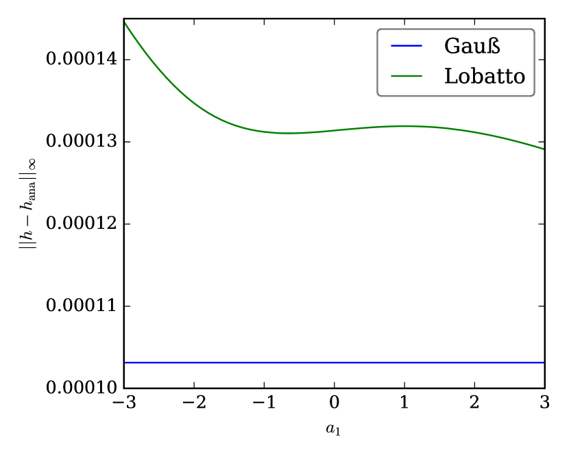
(b) Error $\mathinner{\!\left\lVert h-h_{\mathrm{ana}}\right\rVert}_{\infty}$.

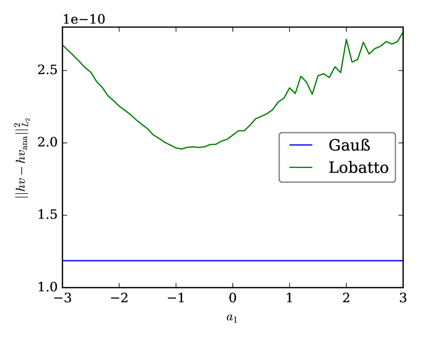
(c) Error $\mathinner{\!\left\lVert hv-hv_{\mathrm{ana}}\right\rVert}_{L_{2}}^{2}$.

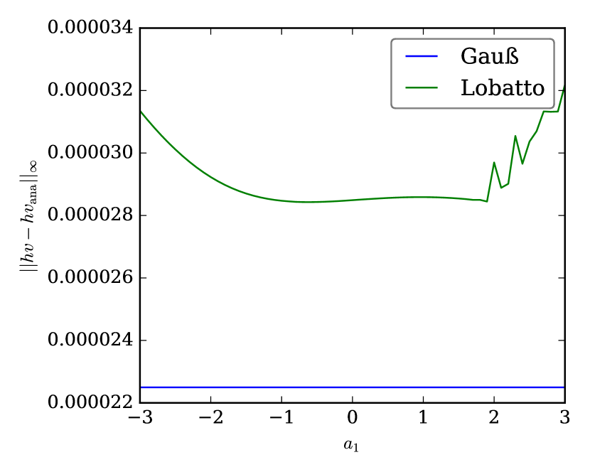
(d) Error $\mathinner{\!\left\lVert hv-hv_{\mathrm{ana}}\right\rVert}_{\infty}$.

Figure 8: Errors of the numerical solution for varying parameter $a_{1}$ and $N=50$ elements of polynomials of degree $\leq p=2$ using Gauß and Lobatto nodes.

(a) Error $\mathinner{\!\left\lVert h-h_{\mathrm{ana}}\right\rVert}_{L_{2}}^{2}$.

(b) Error $\mathinner{\!\left\lVert h-h_{\mathrm{ana}}\right\rVert}_{\infty}$.

(c) Error $\mathinner{\!\left\lVert hv-hv_{\mathrm{ana}}\right\rVert}_{L_{2}}^{2}$.

(d) Error $\mathinner{\!\left\lVert hv-hv_{\mathrm{ana}}\right\rVert}_{\infty}$.

Figure 9: Errors of the numerical solution for varying parameter $a_{1}$ and $N=100$ elements of polynomials of degree $\leq p=2$ using Gauß and Lobatto nodes.

In these experiments, Gauß nodes yield a lower error in the solutions, both in $\mathinner{\!\left\lVert\cdot\right\rVert}_{L_{2}}$ and $\mathinner{\!\left\lVert\cdot\right\rVert}_{\infty}$ and this error is nearly independent of the parameter $a_{1}$ (it varies at most three orders of magnitude lower). However, the error using Lobatto nodes are influenced by the choice of $a_{1}$ with variations up to $\mathrm{5}\mathrm{0}$%.

The corresponding errors in both norms $\mathinner{\!\left\lVert\cdot\right\rVert}_{L_{2}}$ and $\mathinner{\!\left\lVert\cdot\right\rVert}_{\infty}$ follow approximately the same trend for $h$ and $hv$, respectively, but there are differences between the error curves of the height $h$ and the discharge $hv$.

These results, especially the ones for the discharge $hv$, suggest, that choosing the parameter $a_{1}$ between $-1$ and $0$ might be optimal, but this has to be investigated thoroughly.

Remark 22

In the research code used for the simulations, the implementation has not been optimised for maximal performance or adapted to the special nodes. Instead, simple matrix vector products have been evaluated. However, if all possibilities for optimisation are used, the increased accuracy of Gauß nodes has to be compared to the increased computational performance of Lobatto nodes. Thus, especially for two-dimensional and unstructured grids, the choice of Lobatto nodes as used by Wintermeyer et al (2016) seems to be superior. However, the influence of the parameter $a_{1}$ in this case would have to be investigated.

10 Summary and conclusions

A new two-parameter family of entropy stable and well-balanced numerical fluxes and corresponding split forms with adapted surface terms for general SBP bases including Lobatto and Gauß nodes has been developed. The positivity preserving framework of Zhang and Shu (2011) can be used in this setting, but has to be accompanied by some additional dissipation / stabilisation mechanism near wet-dry fronts. Here, the subcell finite volume framework has been used and extended naturally to diagonal-norm nodal SBP bases.

Numerical tests confirm the properties of the derived schemes. As suggested by a first physicists intuition, the second parameter of the two-parameter family should be chosen as $a_{1}=\frac{2-a_{1}}{3}$ in order not to use some higher order terms in the velocity $v$. This choice has been advantageous for the considered moving water equilibrium in section 9.3.

However, the choice of the first parameter $a_{1}$ does not seem to be similarly simple. There is no clear physical intuition at first and the dam break experiments in section 9.4 are not unambiguous. Thus, further analytical and numerical studies have to be performed in order to understand the influence of this parameter and possible optimal choices.

However, since the additional correction terms allowing the use of Gauß nodes become more and more complicated, the gain in accuracy does not seem to justify the use of these. Therefore, the computationally efficient flux differencing form using Lobatto nodes seems to be advantageous. However, this does not confine the results about positivity preservation and both entropy stability and well-balancedness of the new two-parameter family of numerical fluxes. These can be expected to be extendable to two-dimensional unstructured and curvilinear grids using tensor product bases on quadrilaterals similarly to Wintermeyer et al (2016).

Additional topics of further research include the investigation of interactions of curved elements with the parameter $a_{1}$, of other means performing finite volume subcell projection, and other stabilisation techniques.