Extended Skew-Symmetric Form for Summation-by-Parts Operators and Varying Jacobians

Abstract

A generalised analytical notion of summation-by-parts (SBP) methods is proposed, extending the concept of SBP operators in the correction procedure via reconstruction (CPR), a framework of high-order methods for conservation laws. For the first time, SBP operators with dense norms and not including boundary points are used to get an entropy stable split-form of Burgers’ equation. Moreover, overcoming limitations of the finite difference framework, stability for curvilinear grids and dense norms is obtained for SBP CPR methods by using a suitable way to compute the Jacobian.

mo#2#1#2 #1 

1 Introduction

Conservation laws can be used to model many physical phenomena. However, the efficient numerical solution of these equations is difficult, since stability becomes difficult to guarantee for high-order methods.

Here, the concept of summation-by-parts (SBP) operators in the correction procedure via reconstruction (CPR) framework is extended by a new analytical notion of these schemes. For the first time, both nodal and modal SBP bases not including boundary points can be used to construct entropy stable and conservative approximations of Burgers’ equation using an extended skew-symmetric form. Moreover, these dense norm bases can be coupled with curvilinear grids by a suitable way to compute the Jacobian in SBP CPR methods, contrary to classical finite difference SBP schemes.

SBP operators originate in the finite difference (FD) framework and yield an approach to prove stability in a way similar to the continuous investigations by mimicking integration-by-parts on a discrete level, see inter alia the review articles [21, 2] and references cited therein. To get conservation and stability, (exterior and inter-element) boundary conditions are imposed weakly by simultaneous approximation terms (SATs) and skew-symmetric formulations for nonlinear conservation laws are used [3].

Gassner [4] applied the SBP framework to a discontinuous Galerkin (DG) spectral element method (DGSEM) using the nodes of Lobatto-Legendre quadrature. Additionally, Fernández et al. [1] proposed an extended definition of SBP methods in a numerical framework relying on nodal representations.

Ranocha et al. [19] investigated connections between SBP methods and the general CPR framework, unifying flux reconstruction [9] and lifting collocation penalty [26] schemes. Several high-order methods such as DG, spectral volume and spectral difference methods can be formulated in this framework, as described in the review article [10] and references cited therein.

In this article, a brief review of SBP CPR methods is given in section 2, followed by an introduction to some results about a skew-symmetric splitting for diagonal norm bases.

The main contribution of this article will be presented in section 3. There, a more general setting for SBP CPR methods will be described. Based on this, an extended skew-symmetric form of Burgers’ equation is proposed. Extending the correction terms in this form, conservation and nonlinear entropy stability are proved for general SBP CPR semidiscretisations, including both nodal bases without boundary nodes (e.g. Gauß-Legendre nodes) and modal bases (e.g. Legendre polynomials). Numerical examples are presented thereafter. Additionally, a brief comparison with the numerical setting of Fernández et al. [1] is given.

Moreover, limitations of the application of dense norms for curvilinear grids known in FD SBP methods are overcome for SBP CPR methods in section 4.

Finally, the results are summarised in section 5, followed by a discussion and further topics of research.

2 Correction procedure via reconstruction using diagonal-norm SBP operators

In this section, the basic concept and results about summation-by-parts operators for correction procedure via reconstruction of [19] are briefly reviewed.

CPR schemes are designed as semidiscretisations of hyperbolic conservation laws

$$\partial_{t}u+\partial_{x}f(u)=0,$$ (1)

equipped with appropriate initial and boundary conditions. The domain is divided into non-overlapping intervals and each interval is mapped to the reference element $[-1,1]$ for the computations. In each element, a nodal polynomial basis $\mathcal{B}$ of order $p$ is used to represent the numerical solution. The semidiscretisation of (1) (i.e. the computation of $\partial_{x}f(u)$) consists of the following steps, see also the review [10] and references cited therein:

• Interpolate the solution $u$ to the cell boundaries at $-1$ and $1$ (if these values are not already given as coefficients of the nodal basis).

• Compute common numerical fluxes $f^{\mathrm{num}}$ at each cell boundary.

• Compute the flux $f(u)$ pointwise in each node.

• Interpolate the flux $f(u)$ to the boundary and add polynomial correction functions $g_{L}$, $g_{R}$ of degree $p+1$, multiplied by the difference $f_{L/R}-f^{\mathrm{num}}_{L/R}$ of the flux and the numerical flux at the corresponding boundary.

• Finally, compute the resulting derivative of $f+(f_{L}-f^{\mathrm{num}}_{L})g_{L}+(f_{R}-f^{\mathrm{num}}_{R})g_{R}$, using exact differentiation for the polynomial basis.

For the representation of a diagonal-norm SBP operator, the basis $\mathcal{B}$ has to be associated with a quadrature rule, given by nodes $z_{0},\dots,z_{p}$ and appropriate positive weights $\omega_{0},\dots,\omega_{p}$. The values of $u$ at the nodes are the coefficients of the local expansion, i.e. $\underline{u}=(u(z_{0}),\dots,u(z_{p}))^{T}$. The quadrature weights determine a positive definite mass matrix $\mat{M}=\operatorname{diag}(\omega_{0},\dots,\omega_{p})$ associated with a discrete norm $\mathinner{\!\left\lVert u\right\rVert}_{M}^{2}=\underline{u}^{T}\mat{M}\underline{u}$. Moreover, the derivative is represented by the matrix $\mat{D}$ and the restriction to the boundary $\mathinner{\left\{-1,1\right\}}$ of the standard element $[-1,1]$ is performed by the restriction matrix $\mat{R}$. For nodal bases including boundary points (e.g. Lobatto-Legendre nodes), it is given by $\mat{R}=\begin{pmatrix}1&0&\dots&0\\ 0&\dots&0&1\end{pmatrix}$. The bilinear form giving the difference of boundary values is represented by the matrix $\mat{B}=\operatorname{diag}(-1,1)$.

The basis and its associated quadrature rule must satisfy the SBP property

$$\mat{M}\mat{D}+\mat{D}[^{T}]\mat{M}=\mat{R}[^{T}]\mat{B}\mat{R},$$ (2)

in order to mimic integration by parts on a discrete level

$$\int_{-1}^{1}u\,(\partial_{x}v)\operatorname{d\!}x+\int_{-1}^{1}(\partial_{x}u)\,v\operatorname{d\!}x\approx\underline{u}^{T}\mat{M}\mat{D}\underline{v}+(\mat{D}\underline{u})^{T}\mat{M}\underline{v}=(\mat{R}\underline{u})^{T}\mat{B}(\mat{R}\underline{v})\approx\mathinner{u\,v\Bigr{\rvert}}_{-1}^{1}.$$ (3)

If the quadrature is exact for polynomials of degree $\leq 2p-1$, this condition is fulfilled, since all integrals are evaluated exactly, see also [13, 8].

[19] introduced a formulation of CPR methods with special attention paid to SBP operators. After mapping each element to the standard element $[-1,1]$, a CPR method can be formulated as

$$\partial_{t}\underline{u}+\mat{D}\underline{f}+\mat{C}(\underline{f}^{\mathrm{num}}-\mat{R}\underline{f})=0.$$ (4)

Thus, for a given standard element, a CPR method is parametrised by

• A basis $\mathcal{B}$ for the local expansion, determining the derivative and restriction (interpolation) matrices $\mat{D}$ and $\mat{R}$.

• A correction matrix $\mat{C}$, adapted to the chosen basis.

As an example, consider Gauß-Lobatto-Legendre integration with its associated basis of point values at Lobatto nodes in $[-1,1]$. Using the special choice $\mat{C}=\mat{M}[^{-1}]\mat{R}[^{T}]\mat{B}$ and defining $\mat{\widetilde{B}}\mathrel{\mathop{\ordinarycolon}}=\mat{R}[^{T}]\mat{B}\mat{R}$, i.e. $\mat{\widetilde{B}}=\operatorname{diag}(-1,0,\dots,0,1)$, the CPR method of equation (4) reduces to

$$\partial_{t}\underline{u}+\mat{D}\underline{f}+\mat{M}[^{-1}]\mat{\widetilde{B}}\left(\underline{\widetilde{f}}^{\mathrm{num}}-\underline{f}\right)=0,$$ (5)

where $\underline{\widetilde{f}}^{\mathrm{num}}=(f^{\mathrm{num}}_{L},0,\dots,0,f^{\mathrm{num}}_{R})$ contains the numerical flux at the left and right boundary and satisfies $\underline{f}^{\mathrm{num}}=\mat{R}\underline{\widetilde{f}}^{\mathrm{num}}$. Equation (5) is the strong form of the DGSEM formulation of Gassner [4], which he proved to be a diagonal norm SBP operator.

2.1 Results about the skew-symmetric form of Burgers’ equation and diagonal-norm SBP operators

Stability properties for linear and nonlinear problems can be very different. [19] considered Burgers’ equation

$$\partial_{t}u+\partial_{x}\frac{u^{2}}{2}=0$$ (6)

in one space dimension with periodic boundary conditions and appropriate initial condition.

As described by [4], a split-operator form of the flux divergence $\alpha\partial_{x}\frac{1}{2}u^{2}+(1-\alpha)u\partial_{x}u$ can be used to get conservation and stability (across elements) if boundary nodes are included in the basis and the numerical flux is entropy stable in the sense of Tadmor [22, 23], i.e. $\frac{1}{6}(u_{-}^{3}-u_{+}^{3})-(u_{-}-u_{+})f^{\mathrm{num}}(u_{-},u_{+})\leq 0$. Here, the numerical flux $f^{\mathrm{num}}(u_{-},u_{+})$ is computed given the values of $u$ from the elements to the left $(u_{-})$ and to the right ($u_{+}$) of a given boundary. This strong form discontinuous Galerkin spectral element method of [4] with the choice $\alpha=\frac{2}{3}$ can be written as the following semidiscretisation of the skew-symmetric form of Burgers’ equation

$$\partial_{t}\underline{u}+\mat{D}\frac{1}{2}\underline{u^{2}}+\underbrace{\frac{1}{3}\left(\mat{u}\mat{D}\underline{u}-\frac{1}{2}\mat{D}\mat{u}\underline{u}\right)}_{=\mathrel{\mathop{\ordinarycolon}}\underline{c}_{\mathrm{div}}}+\mat{M}[^{-1}]\mat{R}[^{T}]\mat{B}\left(\underline{f}^{\mathrm{num}}-\mat{R}\frac{1}{2}\underline{u^{2}}\right)=\underline{0},$$ (7)

where the vector $\underline{f}^{\mathrm{num}}=(f^{\mathrm{num}}_{L},f^{\mathrm{num}}_{R})$ contains the numerical fluxes at the left and right boundaries of the element. The term $\underline{c}_{\mathrm{div}}$ is a a discrete correction to the divergence term, that has to be used since the product rule is not valid discretely.

For a general SBP basis without boundary nodes, the stability investigation is more complicated. [19] introduced and analysed a new correction term $\underline{c}_{\mathrm{res}}$ for the restriction to the boundary, resulting in

$$\partial_{t}\underline{u}+\mat{D}\frac{1}{2}\underline{u^{2}}+\underline{c}_{\mathrm{div}}+\mat{M}[^{-1}]\mat{R}[^{T}]\mat{B}\left(\underline{f}^{\mathrm{num}}-\mat{R}\frac{1}{2}\underline{u^{2}}-\underline{c}_{\mathrm{res}}\right)=\underline{0},$$ (8)

$$\underline{c}_{\mathrm{div}}=\frac{1}{3}\left(\mat{u}\mat{D}\underline{u}-\frac{1}{2}\mat{D}\mat{u}\underline{u}\right),\qquad\underline{c}_{\mathrm{res}}=\frac{1}{6}\left((\mat{R}\underline{u})^{2}-\mat{R}\mat{u}\underline{u}\right).$$ (9)

It has been stressed that not only the product rule is not valid discretely, but multiplication is not exact. This results in incorrect divergence and restriction terms that have to be corrected in order to get the desired conservation and stability estimates.

Theorem 1 (Theorem 9 of [19]).

If the numerical flux $f^{\mathrm{num}}$ satisfies

$$\frac{1}{6}(u_{-}^{3}-u_{+}^{3})-(u_{-}-u_{+})f^{\mathrm{num}}(u_{-},u_{+})\leq 0,$$ (10)

then a diagonal-norm SBP CPR method (8) with correction terms for both divergence and restriction to the boundary (9) for the inviscid Burgers’ equation (6) is both conservative and stable in the discrete norm $\mathinner{\!\left\lVert\cdot\right\rVert}_{M}$ induced by $\mat{M}$. Numerical fluxes fulfilling condition (10) are inter alia

• the energy conservative (ECON) flux

  $$f^{\mathrm{num}}(u_{-},u_{+})=\frac{1}{4}(u_{+}^{2}+u_{-}^{2})-\frac{(u_{+}-u_{-})^{2}}{12}$$ (11)

• the local Lax-Friedrichs (LLF) flux

  $$f^{\mathrm{num}}(u_{-},u_{+})=\frac{1}{4}(u_{+}^{2}+u_{-}^{2})-\frac{\max(|u_{+}|,|u_{-}|)}{2}(u_{+}-u_{-})$$ (12)

• and Osher’s flux

  $$f^{\mathrm{num}}(u_{-},u_{+})=\begin{dcases}\frac{u_{-}^{2}}{2},&u_{+},u_{-}>0,\\ \frac{u_{+}^{2}}{2},&u_{+},u_{-}<0,\\ \frac{u_{+}^{2}}{2}+\frac{u_{-}^{2}}{2},&u_{-}\geq 0\geq u_{+},\\ 0,&u_{-}\leq 0\leq u_{+}.\end{dcases}$$ (13)

3 Abstract view and generalisation

The basic setting described in the previous section uses diagonal norm SBP operators and nodal bases, associated with quadrature rules with positive weights. These operators have been used in the context of CPR methods to obtain conservative and stable semidiscretisations for linear advection and Burgers’ equation. This chapter provides a more abstract view on the results and generalised schemes with a new form of the correction terms, allowing both modal and nodal bases with arbitrary (dense) norm.

3.1 Analytical setting in one dimension

Continuing the investigations, an analytical setting in the one-dimensional standard element $\Omega=[-1,1]$ is presented at first. The semidiscretisation in space consists of the representation of a numerical solution in a (real) finite dimensional Hilbert space $X_{V}$, the space of functions on the (one-dimensional) volume $\Omega$. Hitherto, $X_{V}$ has been the space of polynomials of degree $\leq p$, i.e. $\dim X_{V}=p+1$. $X_{V}$ is equipped with a suitable basis $\mathcal{B}_{V}$, e.g. a Lagrange (interpolation) basis for Gauß-Legendre or Lobatto-Legendre quadrature nodes. With regard to $\mathcal{B}_{V}$, the scalar product and associated norm on $X_{V}$ are given by a symmetric and positive-definite matrix $\mat{M}$, approximating the $L^{2}$ norm on $X_{V}$, i.e.

$$\underline{u}^{T}\mat{M}\underline{v}=\left\langle\underline{u},\underline{v}\right\rangle_{M}\approx\int_{\Omega}uv=\left\langle u,v\right\rangle_{L^{2}}.$$ (14)

In one dimension, a divergence (derivative) operator mapping $X_{V}$ to $X_{V}$ is represented by a matrix $\mat{D}$.

Besides $X_{V}$, the vector space $X_{B}$ of functions on the ($0$-dimensional) boundary $\partial\Omega$ of the standard element $\Omega$ is used. The associated basis is denoted by $\mathcal{B}_{B}$. In the simple one-dimensional case, $X_{B}$ is a two-dimensional vector space and $\mathcal{B}_{B}$ is chosen to represent point values at $-1$ and $1$. On the boundary, a bilinear form is represented by a matrix $\mat{B}$, approximating the boundary (surface) integral in the outward normal direction, i.e. evaluation at the boundary. More precisely, $\mat{B}$ maps $X_{B}\times X_{B}$ to $\mathbb{R}$ and

$$\underline{u}_{B}^{T}\mat{B}\underline{f}_{B}=B(u_{B},f_{B})\approx\mathinner{u_{B}\,f_{B}\Bigr{\rvert}}_{-1}^{1}.$$ (15)

In the simple one-dimensional setting, $u_{B}$ and $f_{B}$ are both scalar functions and $\int_{\partial\Omega}u_{B}\,f_{B}\cdot n=u(1)f(1)-u(-1)f(-1)$, i.e. $\mat{B}=\operatorname{diag}(-1,1)$ if $\mathcal{B}_{B}$ is ordered such that the value at $-1$ is the first coefficient. With regard to the chosen bases $\mathcal{B}_{V}$ and $\mathcal{B}_{B}$, a restriction operator is represented by a matrix $\mat{R}$, mapping a function $u$ on the volume to its values at the boundary. Again, the SBP property $\mat{M}\mat{D}+\mat{D}[^{T}]\mat{M}=\mat{R}[^{T}]\mat{B}\mat{R}$ (2) mimics integration by parts.

A CPR method is further parametrised by a correction or penalty operator, represented by a matrix $\mat{C}$ adapted to the chosen bases. The canonical choice is $\mat{C}=\mat{M}[^{-1}]\mat{R}[^{T}]\mat{B}$ as described in [19], especially for nonlinear equations. For linear advection, other choices of $\mat{C}$ are possible, recovering the full range of linearly stable schemes presented in [25], see [19, section 3].

Since nonlinear fluxes $f(u)$ appear and are of interest, nonlinear operations on $X_{V}$ have to be described. In general, if $X_{V}$ is a finite-dimensional vector space of polynomials containing polynomials of degree $\leq p$ ($p\geq 1$ and $p$ is minimal), then the product of $u,v\in X_{V}$ is a polynomial of degree $\leq 2p$, i.e. not in $X_{V}$ in general. Therefore, discrete multiplication is not exact. Thus, multiplying $v\in X_{V}$ with $u\in X_{V}$ yields $\mat{u}[^{+}]\underline{v}\in X_{V}^{+}$, where $X_{V}^{+}\supset X_{V}$ is a vector space of higher dimension. After this exact multiplication, a projection on $X_{V}$ is performed, resulting in $\mat{u}\underline{v}\in X_{V}$.

For a nodal basis $\mathcal{B}_{V}$, the natural projection is given by pointwise evaluation at the nodes. However, for a modal basis of Legendre polynomials, the natural projection is an $L^{2}$ orthogonal projection on $X_{V}$. Disappointingly, this concept does not easily extend to division, since $L^{2}$ projection of rational functions is not a simple task.

3.2 Revisiting Burgers’ equation

Investigating again a skew-symmetric SBP CPR method without the assumption of a nodal and/or orthogonal basis, some further complications arise. In contrast to the manipulations used to prove Theorem 1 (see also [4]), $\mat{u}$ and $\mat{M}$ might not commute, either because the nodal basis is not orthogonal or because a modal basis is chosen. Therefore, the correction terms (9) for the divergence and restriction do not suffice to prove conservation and stability. The reason is again inexactness of discrete multiplication. A multiplication operator $\mat{u}$ should be self-adjoint, at least in a finite-dimensional space (and in general, if a correct domain is chosen). Thus, instead of $\mat{u}$ in the first term of $\underline{c}_{\mathrm{div}}$, the adjoint $\mat{u}[^{*}]$ of $\mat{u}$ with respect to the scalar product induced by $\mat{M}$ is proposed. The symmetry condition

$$\left\langle\underline{v},\mat{u}\underline{w}\right\rangle_{M}=\left\langle\mat{u}[^{*}]\underline{v},\underline{w}\right\rangle_{M}$$ (16)

can be written as

$$\underline{v}^{T}\mat{M}\mat{u}\underline{w}=\underline{v}^{T}(\mat{u}[^{*}])^{T}\mat{M}\underline{w}.$$ (17)

Thus, since $\underline{v}$ and $\underline{w}$ are arbitrary, $\mat{M}\mat{u}=(\mat{u}[^{*}])^{T}\mat{M}$, i.e. $\mat{u}[^{*}]=\mat{M}[^{-1}]\mat{u}[^{T}]\mat{M}$, and the generalised correction terms are

$$\underline{c}_{\mathrm{div}}=\frac{1}{3}\left(\mat{M}[^{-1}]\mat{u}[^{T}]\mat{M}\mat{D}\underline{u}-\frac{1}{2}\mat{D}\mat{u}\underline{u}\right),\qquad\underline{c}_{\mathrm{res}}=\frac{1}{6}\left((\mat{R}\underline{u})^{2}-\mat{R}\mat{u}\underline{u}\right).$$ (18)

Using these correction terms, Theorem 1 is generalised by

Theorem 2.

If the numerical flux $f^{\mathrm{num}}$ satisfies $\frac{1}{6}(u_{-}^{3}-u_{+}^{3})-(u_{-}-u_{+})f^{\mathrm{num}}(u_{-},u_{+})\leq 0$ (10), then a general SBP CPR method with $\mat{C}=\mat{M}[^{-1}]\mat{R}[^{T}]\mat{B}$ and correction terms (18) for both divergence and restriction to the boundary

$$\partial_{t}\underline{u}+\mat{D}\frac{1}{2}\underline{u^{2}}+\underline{c}_{\mathrm{div}}+\mat{C}\left(\underline{f}^{\mathrm{num}}-\mat{R}\frac{1}{2}\underline{u^{2}}-\underline{c}_{\mathrm{res}}\right)=\underline{0},$$ (19)

for the inviscid Burgers’ equation (6) is both conservative and stable across elements in the discrete norm $\mathinner{\!\left\lVert\cdot\right\rVert}_{M}$ induced by $\mat{M}$. Numerical fluxes fulfilling condition (10) are inter alia

• the energy conservative (ECON) flux (11),

• the local Lax-Friedrichs (LLF) flux (12),

• and Osher’s flux (13).

Proof.

Multiplying $\partial_{t}\underline{u}$ with $\underline{v}^{T}\mat{M}$, inserting $\mat{C}=\mat{M}[^{-1}]\mat{R}[^{T}]\mat{B}$ and applying the SBP property (2) yields

$$\underline{v}^{T}\mat{M}\partial_{t}\underline{u} =-\frac{1}{2}\underline{v}^{T}\mat{M}\mat{D}\mat{u}\underline{u}-\underline{v}^{T}\mat{M}\underline{c}_{\mathrm{div}}-\underline{v}^{T}\mat{R}[^{T}]\mat{B}\left(\underline{f}^{\mathrm{num}}-\frac{1}{2}\mat{R}\mat{u}\underline{u}-\underline{c}_{\mathrm{res}}\right)$$ (20)

$$=+\frac{1}{2}\underline{v}^{T}\mat{D}[^{T}]\mat{M}\mat{u}\underline{u}-\frac{1}{2}\underline{v}^{T}\mat{R}[^{T}]\mat{B}\mat{R}\mat{u}\underline{u}$$

$$\quad-\underline{v}^{T}\mat{M}\underline{c}_{\mathrm{div}}-\underline{v}^{T}\mat{R}[^{T}]\mat{B}\left(\underline{f}^{\mathrm{num}}-\frac{1}{2}\mat{R}\mat{u}\underline{u}-\underline{c}_{\mathrm{res}}\right).$$

Gathering terms and inserting $\underline{c}_{\mathrm{div}}$, $\underline{c}_{\mathrm{res}}$ from equation (18) results in

$$\underline{v}^{T}\mat{M}\partial_{t}\underline{u} =\frac{1}{2}\underline{v}^{T}\mat{D}[^{T}]\mat{M}\mat{u}\underline{u}-\underline{v}^{T}\mat{M}\underline{c}_{\mathrm{div}}-\underline{v}^{T}\mat{R}[^{T}]\mat{B}\underline{f}^{\mathrm{num}}+\underline{v}^{T}\mat{R}[^{T}]\mat{B}\underline{c}_{\mathrm{res}}$$ (21)

$$=\frac{1}{2}\underline{v}^{T}\mat{D}[^{T}]\mat{M}\mat{u}\underline{u}-\frac{1}{3}\underline{v}^{T}\mat{u}[^{T}]\mat{M}\mat{D}\underline{u}+\frac{1}{6}\underline{v}^{T}\mat{M}\mat{D}\mat{u}\underline{u}$$

$$\quad-\underline{v}^{T}\mat{R}[^{T}]\mat{B}\underline{f}^{\mathrm{num}}+\frac{1}{6}\underline{v}^{T}\mat{R}[^{T}]\mat{B}(\mat{R}\underline{u})^{2}-\frac{1}{6}\underline{v}^{T}\mat{R}[^{T}]\mat{B}\mat{R}\mat{u}\underline{u}.$$

Applying the SBP property (2) for the third term yields

$$\underline{v}^{T}\mat{M}\partial_{t}\underline{u} =\frac{1}{2}\underline{v}^{T}\mat{D}[^{T}]\mat{M}\mat{u}\underline{u}-\frac{1}{3}\underline{v}^{T}\mat{u}[^{T}]\mat{M}\mat{D}\underline{u}+\frac{1}{6}\underline{v}^{T}\mat{R}[^{T}]\mat{B}\mat{R}\mat{u}\underline{u}-\frac{1}{6}\underline{v}^{T}\mat{D}[^{T}]\mat{M}\mat{u}\underline{u}$$ (22)

$$\quad-\underline{v}^{T}\mat{R}[^{T}]\mat{B}\underline{f}^{\mathrm{num}}+\frac{1}{6}\underline{v}^{T}\mat{R}[^{T}]\mat{B}(\mat{R}\underline{u})^{2}-\frac{1}{6}\underline{v}^{T}\mat{R}[^{T}]\mat{B}\mat{R}\mat{u}\underline{u}$$

$$=\frac{1}{3}\underline{v}^{T}\mat{D}[^{T}]\mat{M}\mat{u}\underline{u}-\frac{1}{3}\underline{v}^{T}\mat{u}[^{T}]\mat{M}\mat{D}\underline{u}-\underline{v}^{T}\mat{R}[^{T}]\mat{B}\underline{f}^{\mathrm{num}}+\frac{1}{6}\underline{v}^{T}\mat{R}[^{T}]\mat{B}(\mat{R}\underline{u})^{2}.$$

In order to obtain stability, $\frac{1}{2}\dfrac{\operatorname{d\!}{}}{\operatorname{d\!}{t}}\mathinner{\!\left\lVert u\right\rVert}_{M}^{2}=\underline{u}^{T}\mat{M}\partial_{t}\underline{u}$ has to be considered. Thus, setting $\underline{v}=\underline{u}$ in (22) and using the symmetry of the $\mat{M}$ results in

$$\frac{1}{2}\dfrac{\operatorname{d\!}{}}{\operatorname{d\!}{t}}\mathinner{\!\left\lVert u\right\rVert}_{M}^{2}=-\underline{u}^{T}\mat{R}[^{T}]\mat{B}\underline{f}^{\mathrm{num}}+\frac{1}{6}\underline{u}^{T}\mat{R}[^{T}]\mat{B}(\mat{R}\underline{u})^{2},$$ (23)

Denoting the values from the cells left and right to a given boundary node with indices $-$ and $+$, respectively, and summing over all elements, the contribution of one boundary node to $\frac{1}{2}\dfrac{\operatorname{d\!}{}}{\operatorname{d\!}{t}}\mathinner{\!\left\lVert u\right\rVert}_{M}^{2}$ is

$$\frac{1}{6}(u_{-}^{3}-u_{+}^{3})-(u_{-}-u_{+})f^{\mathrm{num}}(u_{-},u_{+}).$$ (24)

If this is non-positive (as assumed), stability in the discrete norm described by $\mat{M}$ is guaranteed.

Investigation conservation by setting $\underline{v}=\underline{1}$ in (22), using $\mat{D}\underline{1}=0$ (i.e. exact differentiation for constant functions) and $\mat{u}\underline{1}=\underline{u}$ (i.e. exact multiplication with constant functions) yields

$$\dfrac{\operatorname{d\!}{}}{\operatorname{d\!}{t}}\underline{1}^{T}\mat{M}\underline{u}=-\frac{1}{3}\underline{u}^{T}\mat{M}\mat{D}\underline{u}-\underline{1}^{T}\mat{R}[^{T}]\mat{B}\underline{f}^{\mathrm{num}}+\frac{1}{6}\underline{1}^{T}\mat{R}[^{T}]\mat{B}(\mat{R}\underline{u})^{2}.$$ (25)

Rewriting the first term (by the SBP property (2)) as

$$-\frac{1}{3}\underline{u}^{T}\mat{M}\mat{D}\underline{u}=-\frac{1}{6}\underline{u}^{T}\mat{M}\mat{D}\underline{u}+\frac{1}{6}\underline{u}^{T}\mat{D}[^{T}]\mat{M}\underline{u}-\frac{1}{6}\underline{u}^{T}\mat{R}[^{T}]\mat{B}\mat{R}\underline{u}=-\frac{1}{6}\underline{u}^{T}\mat{R}[^{T}]\mat{B}\mat{R}\underline{u}$$ (26)

results in

$$\dfrac{\operatorname{d\!}{}}{\operatorname{d\!}{t}}\underline{1}^{T}\mat{M}\underline{u}=-\frac{1}{6}\underline{u}^{T}\mat{R}[^{T}]\mat{B}\mat{R}\underline{u}-\underline{1}^{T}\mat{R}[^{T}]\mat{B}\underline{f}^{\mathrm{num}}+\frac{1}{6}\underline{1}^{T}\mat{R}[^{T}]\mat{B}(\mat{R}\underline{u})^{2}.$$ (27)

Denoting the values of $u$ at the left and right boundary as $u_{L}$ and $u_{R}$, respectively,

$$\underline{u}^{T}\mat{R}[^{T}]\mat{B}\mat{R}\underline{u}=u_{R}\cdot u_{R}-u_{L}\cdot u_{L}=1\cdot u_{R}^{2}-1\cdot u_{L}^{2}=\underline{1}^{T}\mat{R}[^{T}]\mat{B}(\mat{R}\underline{u})^{2}.$$ (28)

and therefore

$$\dfrac{\operatorname{d\!}{}}{\operatorname{d\!}{t}}\underline{1}^{T}\mat{M}\underline{u}=-\underline{1}^{T}\mat{R}[^{T}]\mat{B}\underline{f}^{\mathrm{num}}.$$ (29)

Thus, summing over all elements, the contribution of both cells sharing a common boundary node cancel each other, since the numerical flux $f^{\mathrm{num}}$ is the same for both elements. ∎

Remark 3.

In Theorem 2, conservation across elements has been considered. On a sub-element level, conservation for diagonal-norm SBP operators including boundary nodes has been proven in [3] in the context of the Lax-Wendroff theorem. An extension to dense norm and modal bases is still an open question.

Remark 4.

Regarding conservation and stability across elements, Theorem 2 is very general. However, there are several special cases that deserve to be mentioned explicitly for comparison and a better understanding.

1. Nodal bases including boundary nodes with diagonal mass matrix.
   This has been considered inter alia in [4]. Since boundary nodes are included, the correction term for the restriction vanishes, $\underline{c}_{\mathrm{res}}=\underline{0}$. Moreover, since the mass matrix $\mat{M}$ and the multiplication operators $\mat{u}$ are diagonal, the $\mat{M}$-adjoint is simply $\mat{u}[^{*}]=\mat{M}[^{-1}]\mat{u}[^{T}]\mat{M}=\mat{u}^{T}=\mat{u}$.

2. Nodal bases (possibly not including boundary nodes) with diagonal mass matrix.
   This has been considered in [19]. Here, the correction term for the restriction is in general not zero and has to be used to get a conservative and stable scheme. However, the mass matrix $\mat{M}$ and the multiplication operators $\mat{u}$ are diagonal, resulting in $\mat{u}[^{*}]=\mat{u}$.

3. Nodal bases (possibly not including boundary nodes) with general mass matrix.
   Here, both the usage of both correction terms with the correct $\mat{M}$-adjoint $\mat{u}[^{*}]=\mat{M}[^{-1}]\mat{u}[^{T}]\mat{M}$ is necessary in general to get the desired properties of the scheme.

4. Modal Legendre bases.
   In this case, no boundary nodes can be “included”. Thus, the correction term for the restriction to the boundary does not vanish in general. Here, multiplication operators performing exact multiplication followed by an orthogonal projection are considered. For this orthogonal basis, a multiplication operator $\mat{u}$ is in general not diagonal, but $\mat{M}$-self-adjoint, as the following calculation for arbitrary polynomials $u,v,w$ of degree $\leq p$ shows:

   $$\left\langle\underline{v},\mat{u}\underline{w}\right\rangle_{M}=\underline{v}^{T}\mat{M}\mat{u}\underline{w}=\int v\operatorname{proj}(u\,w)=\int v\,u\,w=\int\operatorname{proj}(u\,v)\,w=\underline{v}^{T}\mat{u}[^{T}]\mat{M}\underline{w}=\left\langle\mat{u}\underline{v},\underline{w}\right\rangle_{M}.$$ (30)

   In the second step, the definition of the multiplication operator as exact multiplication followed by an orthogonal projection on the space of polynomials of degree $\leq p$ is inserted. In the following step, this orthogonality is used, since $v$ is a polynomial of degree $\leq p$. Similarly, the orthogonality of Legendre polynomials is used in the fourth step. Thus, multiplication operators $\mat{u}$ are $\mat{M}$-self-adjoint.

Remark 5.

The correction terms used in Theorem 2 can be extended to systems as well. In [5], an entropy stable split form of the shallow water equations has been analysed using Lobatto-Legendre nodes. This has been extended to two-dimensional curvilinear grids in [27] and to a whole two-parameter family of splittings for general SBP bases in [17]. Moreover, a kinetic energy preserving DG method for the Euler equations using a split form has been proposed in [14, 15].

3.3 Numerical results for dense norm and modal bases

Here, Burgers’ equation (6) is considered in the domain $[0,2]$ with periodic boundary conditions . The initial condition

$$u(0,x)=u_{0}(x)=\sin(\pi x)+0.01$$ (31)

is evolved in time using the classical fourth order Runge-Kutta method with $10\,000$ time steps in the time interval $[0,3]$. As semidiscretisation in space, several SBP CPR methods with $N=20$ equally spaced elements describing polynomials of degree $\leq p=7$ and correction terms (18) are used.

As nodal bases with diagonal norm matrix $\mat{M}$, the nodes of Gauß-Legendre and Lobatto-Legendre quadrature rules are used. The new nodal bases represent polynomials of degree $\leq p=7$ using their values at the

• roots $\xi_{i}=\cos\frac{(2i+1)\pi}{2p+2},\,i=0,\dots,p$,

• extrema $\xi_{i}=\cos\frac{i\pi}{p},\,i=0,\dots,p$

of Chebyshev polynomial $T_{p+1}$ of first kind or the

• roots $\xi_{i}=\cos\frac{(i+1)\pi}{p+2},\,i=0,\dots,p$

of the Chebyshev polynomial $U_{p+1}$ of second kind. The differentiation and norm matrices $\mat{D}$, $\mat{M}$ are computed via their representation for Legendre polynomials and a basis transformation using the associated Vandermonde matrix, see A. Multiplication is conducted pointwise at the corresponding Chebyshev nodes. For these bases, $\mat{M}$ is not diagonal and multiplication operators $\mat{u}$ are not $\mat{M}$-self-adjoint in general.

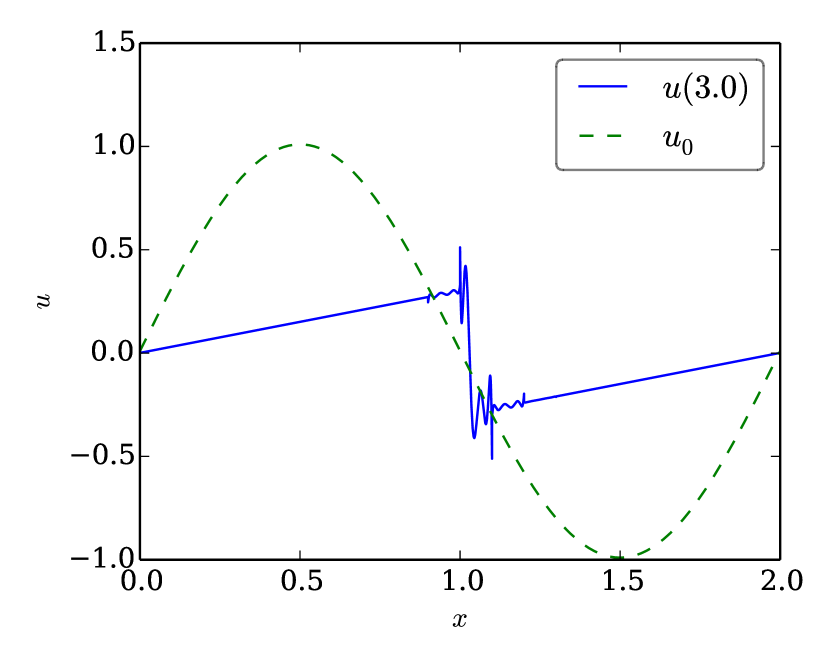
(a) Gauß-Legendre.

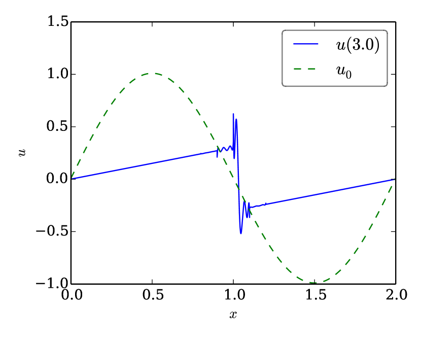
(b) Lobatto-Legendre.

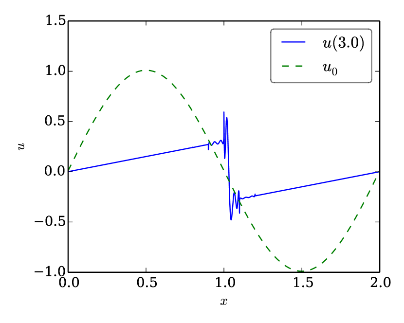
(c) Chebyshev first kind, roots.

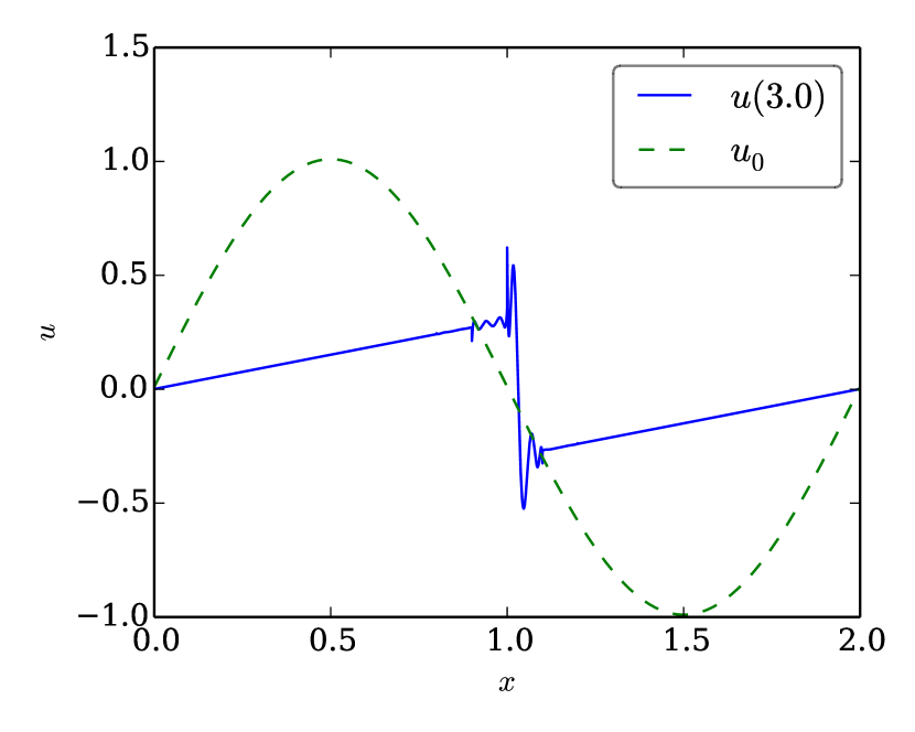
(d) Chebyshev first kind, extrema.

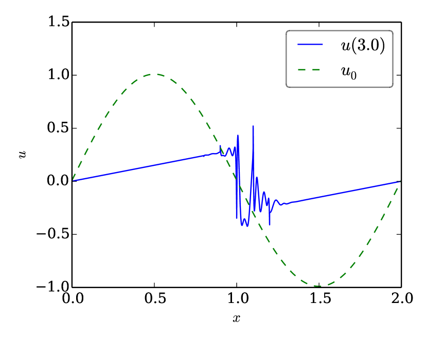
(e) Chebyshev second kind, roots.

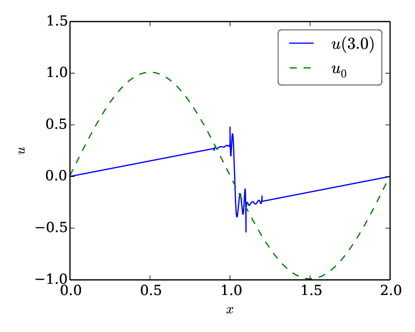
(f) Legendre.

Figure 3: Results of the simulations for Burgers’ equation using general SBP CPR methods with 20 elements, different bases of order 7 and local Lax-Friedrichs (LLF) flux. Corrections for both divergence and restriction are used. Each Figure shows the values of $u(3)$ (blue line) and $u(0)=u_{0}$ (green, dashed) for different bases. (For interpretation of the references to colour in this figure legend, the reader is referred to the web version of this article.)

Additionally, a modal basis of Legendre polynomials as described in Remark 4 is used. An interpolation approach to compute the initial values for a Legendre basis using the nodes of all nodal bases presented in Figure 3 has been used. There is no visual difference between results for these different sets of nodes. In the following, interpolation via Gauß-Legendre nodes has been used.

The momentum and energy of the numerical solutions using the local Lax-Friedrichs flux are shown in Figure 1. For comparison, the results of [19] using Gauß-Legendre and Lobatto-Legendre bases are included in the first rows. The corresponding numerical solutions are given in B, Figure 3, for comparison.

As expected, momentum is conserved for all bases and the discrete energy (entropy) is constant until $t\approx 0.5$ and decays afterwards, as can be seen in Figure 1.

These results are obtained using general SBP CPR methods (19) with both correction terms for divergence and restriction (18). Ignoring a non-trivial correction term for a nodal basis leads to physically useless results, as shown for example by [19, Figure 11]. Results without the skew-symmetric correction $\underline{c}_{\mathrm{div}}$ are not plotted here. Additionally, the correction term $\underline{c}_{\mathrm{div}}$ using the $\mat{M}$-adjoint multiplication operator is verified numerically, since using the simple multiplication as in the previous chapter gives erroneous results, again not shown here.

Remarkably, the results (not plotted here) using a modal Legendre basis and either both or no correction term ($\underline{c}_{\mathrm{div}}$, $\underline{c}_{\mathrm{res}}$) are visually indistinguishable. Additionally, using only $\underline{c}_{\mathrm{res}}$ yields the same results. Contrary, using only a correction for the divergence results in varying momentum and physically useless results. Using an exact orthogonal projection during multiplication seems to be a good idea, but an analytical investigation of this phenomenon remains an open problem.

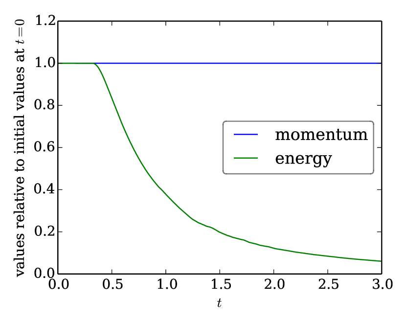
(a) Gauß-Legendre.

(b) Lobatto-Legendre.

(c) Chebyshev first kind, roots.

(d) Chebyshev first kind, extrema.

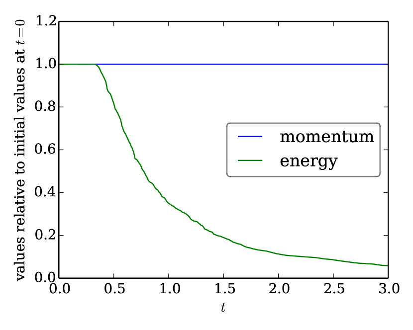
(e) Chebyshev second kind, roots.

(f) Legendre.

Figure 1: Results of the simulations for Burgers’ equation using general SBP CPR methods with 20 elements, different bases of order 7 and local Lax-Friedrichs (LLF) flux. Corrections for both divergence and restriction are used. Each Figure shows the discrete momentum $\underline{1}^{T}\mat{M}\underline{u}$ (blue) and discrete energy $\underline{u}^{T}\mat{M}\underline{u}$ (green) for different bases. (For interpretation of the references to colour in this figure legend, the reader is referred to the web version of this article.)

Remark 6.

These high-order SBP CPR methods should be seen as some entropy stable baseline schemes. If calculations involving shocks are performed, these schemes remain stable and do not crash, but oscillations occur. Therefore, some form of additional shock capturing should be performed, e.g. artificial dissipation or modal filtering [18, 6]. However, this is not the target of this investigation.

3.4 A brief view on a numerical setting

The analytical setting of section 3.1 is based on a given solution space $X_{V}$ for the one-dimensional standard element, since the investigations in this work started from CPR methods, extending DG methods, which are also described by a fundamental basis. Contrary, the theory of SBP operators originates in FD methods, classically not equipped with a solution basis other than the nodal values. Nevertheless, Gassner [4] adapted the SBP framework to a DGSEM with nodal Lobatto-Legendre basis and lumped mass matrix. Additionally, Fernández et al. [1] proposed a generalised SBP framework in one dimension based on nodal values without an analytical basis. Instead, the operators are required to fulfil the SBP property and some accuracy conditions, i.e. they should be exact for polynomials up to some degree $p\geq 1$. These ideas were extended by Hicken et al. [7] to multi-dimensional operators, focussing on diagonal-norm SBP operators on simplex elements in two and three dimensions, i.e. triangles and tetrahedra.

These extensions were applied to linear advection with constant velocity and proved to be conservative and stable in the norm associated with the SBP operator. Relaxing accuracy conditions potentially results in additional free parameters, allowing the construction of specialised schemes for different purposes. As already proved in [8], SBP operators are tightly coupled to quadrature rules. Thus, different quadrature rules can be used to obtain SBP operators and vice versa.

All investigations conducted in the previous chapters and sections directly extend to these generalised FD SBP operators with diagonal or dense norm, respectively. Additionally, since these operators are described by the same matrices used hitherto in the investigations, they can be simply plugged in the numerical method for the calculations – up to the last step.

In the analytical setting, the solution is completely determined by the given coefficients with regard to the chosen basis, i.e. sub-cell resolution of arbitrary accuracy is given. Especially, the solution can be plotted exactly as it is used in the computations. Contrary, using only nodal values at a given set of points without an interpretation as coefficients of a known basis, only these point values can be plotted as output seriously. Performing any interpolation would be a guess, but can in general not describe the solution accurately. From the authors’ point of view, this is a drawback of the numerical setting without a basis as foundation, since high-order methods can generate highly accurate approximations of smooth solutions with few degrees of freedom, see also [12, p. 78, paragraph 2]. However, if the resolution is good enough, a piecewise linear approximation of nodal values used in most plotting software can be sufficient. Thus, depending on the applications, this can also be considered a minor drawback.

The inability to describe a modal basis does not seem to be equally unfavourable, since computing a correct orthogonal projection for division is not a straightforward task and nodal methods are much more efficient regarding evaluation times for nonlinear operations.

A solution of the interpolation problem would be to construct a basis describing a given SBP operator. For example, Gassner [4] constructed a basis for a specially chosen FD SBP operator. However, there does not seem to be a straightforward way to construct such a basis in general.

4 Curvilinear coordinates

For real world applications, simple linear coordinate transformations from the physical element to the reference element might not be enough. Therefore, curvilinear coordinate transformations have to be applied. However, Svärd [20] investigated such transformations in the setting of finite difference SBP operators. As a result, only diagonal norm SBP operators have been used for curvilinear coordinates. Nevertheless, this sections investigates curvilinear coordinates for the linear advection equation with constant coefficients in the setting of SBP CPR methods, also with dense norms.

4.1 Linear advection

The linear advection equation

$$\partial_{t}u+\partial_{x}u=0$$ (32)

with appropriate initial and boundary conditions is used as test problem. Integrating over an interval $\Omega$ yields the integral form

$$\dfrac{\operatorname{d\!}{}}{\operatorname{d\!}{t}}\int_{\Omega}u=\int_{\Omega}\partial_{t}u=-\int_{\Omega}\partial_{x}u=-u\big{|}_{\partial\Omega}.$$ (33)

Similarly, the energy obeys for sufficiently smooth solutions

$$\frac{1}{2}\dfrac{\operatorname{d\!}{}}{\operatorname{d\!}{t}}\mathinner{\!\left\lVert u\right\rVert}_{\Omega}^{2}=\int_{\Omega}u\partial_{t}u=-\int_{\Omega}u\partial_{x}u=-\frac{1}{2}u^{2}\big{|}_{\partial\Omega}.$$ (34)

If a coordinate mapping $x\mapsto\xi$ from the physical element $\Omega$ to a reference element $\hat{\Omega}$ is used, the resulting transport equation is

$$\partial_{t}u+\partial_{x}\xi\,\partial_{\xi}u=0.$$ (35)

Using $J=\partial_{\xi}x=(\partial_{x}\xi)^{-1}$, this can be written as

$$J\partial_{t}u+\partial_{\xi}u=0.$$ (36)

Therefore, integration over the reference element $\hat{\Omega}$ yields

$$\dfrac{\operatorname{d\!}{}}{\operatorname{d\!}{t}}\int_{\Omega}u\operatorname{d\!}x=\dfrac{\operatorname{d\!}{}}{\operatorname{d\!}{t}}\int_{\hat{\Omega}}Ju\operatorname{d\!}\xi=\int_{\hat{\Omega}}J\partial_{t}u\operatorname{d\!}\xi=-\int_{\hat{\Omega}}\partial_{\xi}u\operatorname{d\!}\xi=-u\big{|}_{\partial\Omega}.$$ (37)

Similarly,

$$\frac{1}{2}\dfrac{\operatorname{d\!}{}}{\operatorname{d\!}{t}}\mathinner{\!\left\lVert u\right\rVert}_{\Omega}^{2}=\frac{1}{2}\dfrac{\operatorname{d\!}{}}{\operatorname{d\!}{t}}\int_{\hat{\Omega}}Ju^{2}\operatorname{d\!}\xi=\int_{\hat{\Omega}}Ju\partial_{t}u\operatorname{d\!}\xi=-\int_{\hat{\Omega}}u\partial_{\xi}u\operatorname{d\!}\xi=-\frac{1}{2}u^{2}\big{|}_{\partial\Omega}.$$ (38)

Semidiscretely, the transport equation is approximated on a reference element $\hat{\Omega}$ by

$$\mat{J}\partial_{t}\underline{u}+\mat{D}\underline{u}+\mat{M}[^{-1}]\mat{R}[^{T}]\mat{B}\left(\underline{f}^{\mathrm{num}}-\mat{R}\underline{u}\right)=\underline{0}.$$ (39)

Investigating conservation, the SBP property (2) and exactness of differentiation for constants, i.e. $\mat{D}\underline{1}=0$, can be used to get

$$\underline{1}^{T}\mat{M}\mat{J}\partial_{t}\underline{u}= -\underline{1}^{T}\mat{M}\mat{D}\underline{u}-\underline{1}^{T}\mat{R}[^{T}]\mat{B}\left(\underline{f}^{\mathrm{num}}-\mat{R}\underline{u}\right)$$ (40)

$$= \underline{1}^{T}\mat{D}[^{T}]\mat{M}\underline{u}-\underline{1}^{T}\mat{R}[^{T}]\mat{B}\mat{R}\underline{u}-\underline{1}^{T}\mat{R}[^{T}]\mat{B}\left(\underline{f}^{\mathrm{num}}-\mat{R}\underline{u}\right)=-\underline{1}^{T}\mat{R}[^{T}]\mat{B}\underline{f}^{\mathrm{num}}.$$

Similarly,

$$\underline{u}^{T}\mat{M}\mat{J}\partial_{t}\underline{u}=-\underline{u}^{T}\mat{M}\mat{D}\underline{u}-\underline{u}^{T}\mat{R}[^{T}]\mat{B}\left(\underline{f}^{\mathrm{num}}-\mat{R}\underline{u}\right)$$ (41)

$$= -\frac{1}{2}\underline{u}^{T}\mat{M}\mat{D}\underline{u}+\frac{1}{2}\underline{u}^{T}\mat{D}[^{T}]\mat{M}\underline{u}-\frac{1}{2}\underline{u}^{T}\mat{R}[^{T}]\mat{B}\mat{R}\underline{u}-\underline{u}^{T}\mat{R}[^{T}]\mat{B}\left(\underline{f}^{\mathrm{num}}-\mat{R}\underline{u}\right)=-\underline{u}^{T}\mat{R}[^{T}]\mat{B}\left(\underline{f}^{\mathrm{num}}-\frac{1}{2}\mat{R}\underline{u}\right).$$

To use (41) as an energy estimate, $\mat{M}\mat{J}$ has to be symmetric and positive definite. There are three cases that can be handled differently:

1. If the coordinate transformation $x\mapsto\xi$ satisfies $J=\partial_{\xi}x>0$, a nodal SBP basis with diagonal norm $\mat{M}$ and pointwise multiplication operator $\mat{J}$ is used, both $\mat{M}$ and $\mat{J}$ are diagonal matrices with positive entries on the diagonal. Therefore, $\mat{M}\mat{J}$ is symmetric and positive definite. This is fulfilled inter alia by Gauß-Legendre and Lobatto-Legendre bases.

2. If a modal Legendre basis is used and $\mat{J}$ is given by exact multiplication followed by exact $L^{2}$ projection,

   $$\underline{v}^{T}\mat{M}\mat{J}\underline{u}=\int v\operatorname{proj}(Ju)=\int v\,Ju=\int\operatorname{proj}(Jv)u=\underline{v}^{T}\mat{J}[^{T}]\mat{M}\underline{u},$$ (42)

   since the Legendre polynomials are orthogonal. Thus, $\mat{J}$ is $\mat{M}$-self-adjoint and $\mat{M}\mat{J}=\mat{J}[^{T}]\mat{M}$ is symmetric and positive definite for $J=\partial_{\xi}x>0$.

3. As described in A, coordinate transformations can be used to transform multiplication operators $\mat{J}$ from one basis to another. If $\underline{u},\underline{\hat{u}}$ are vectors represented in different bases and $\mat{V}$ is the corresponding transformation matrix, i.e. $\underline{u}=\mat{V}\underline{\hat{u}}$, the matrices $\mat{J}$ and $\mat{\hat{J}}$ are related via $\mat{\hat{J}}=\mat{V}[^{-1}]\mat{J}\mat{V}$. This can be used to transform the multiplication operator $\mat{J}$ and the mass matrix $\mat{M}$ from a bases in which $\mat{M}\mat{J}$ is symmetric and positive definite [e.g. Gauß-Legendre nodes with diagonal multiplication matrix] to another one [e.g. dense norm Chebyshev bases as in section 3.3].

4.2 Numerical results

The initial condition $u_{0}(x)=\exp\left(-20x^{2}\right)$ of the linear advection equation (32) has been transported in the time interval $[0,4]$ using the classical fourth order Runge-Kutta method. The domain $[-1,1]$ is divided into $5$ elements using polynomials of degree $\leq p=9$ on each element. Here, three different grids have been considered.

• Grid 1: Uniform widths $\Delta x_{i}=\Delta x_{i-1}$, $i\in\mathinner{\left\{2,3,4,5\right\}}$.

• Grid 2: Alternating widths $\Delta x_{i}=10\Delta x_{i-1}$ for $i\in\mathinner{\left\{3,5\right\}}$ and $\Delta x_{i}=\frac{1}{10}\Delta x_{i-1}$ for $i\in\mathinner{\left\{2,4\right\}}$.

• Grid 3: Geometrically increasing widths $\Delta x_{i}=\frac{3}{2}\Delta x_{i-1}$, $i\in\mathinner{\left\{2,3,4,5\right\}}$.

As polynomial bases, nodal bases using Gauß-Legendre and Lobatto-Legendre nodes as well as the roots of the Chebyshev polynomials $U_{p+1}$ of second kind have been chosen. As numerical flux, the central flux $f^{\mathrm{num}}(u_{-},u_{+})=\frac{u_{-}+u_{+}}{2}$ is used.

Two kinds of (local) mappings from the reference element $[-1,1]$ to each of the five physical elements $[x_{\mathrm{min}},x_{\mathrm{max}}]$ have been chosen:

• The standard linear mapping $[-1,1]\ni\xi\mapsto\frac{x_{\mathrm{max}}+x_{\mathrm{min}}}{2}+\xi\frac{x_{\mathrm{max}}-x_{\mathrm{min}}}{2}$.

• The quadratic mapping $[-1,1]\ni\xi\mapsto\frac{x_{\mathrm{max}}-x_{\mathrm{min}}}{8}(\xi+2)^{2}+x_{\mathrm{min}}-\frac{x_{\mathrm{max}}-x_{\mathrm{min}}}{8}$.

Computing $\partial_{\xi}x$ via differentiation of the interpolation polynomial, two versions for the computation of $\mat{J}$ have been conducted:

• As diagonal multiplication operator $\operatorname{diag}(\partial_{\xi}x\big{|}_{\xi=\xi_{i}})$.

• As $\mat{V}\mat{\tilde{J}}\mat{V}[^{-1}]$, where $\mat{\tilde{J}}$ is the diagonal Jacobian in a basis using Gauß-Legendre nodes.

The numerical results for the linear mapping and all choices considered here are visually indistinguishable from the initial data which are also the solution at $t=4$. Therefore, these results are not shown here.

However, if the quadratic mapping is used for Chebyshev nodes and $\mat{J}$ is computed as diagonal multiplication matrix, the numerical solution blows up. If the stable choice of computing $\mat{J}$ via Gauß-Legendre nodes is used, the solution is visually the same as the one for the linear mapping, as can be seen in Figure 2 [cf. case 3. in the previous section].

Similarly, if the diagonal multiplication matrix $\mat{J}$ is used for Lobatto-Legendre nodes, the solutions is stable [cf. case 1. in the previous section]. However, since the lumped mass matrix is not exact as for Gauß-Legendre nodes, computing $\mat{J}$ via Gauß-Legendre nodes results in a blow up of the numerical solution.

The results are qualitatively independent on the choice of the grid for the three different possibilities described above: If the method is stable, the results are visually indistinguishable from the exact solution. Otherwise, the numerical solutions blows up.

(a) Chebyshev second kind (roots), $\mat{J}$ computed via Gauß-Legendre nodes.

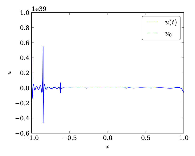
(b) Chebyshev second kind (roots), $\mat{J}$ as diagonal multiplication matrix.

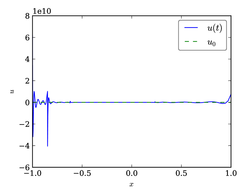
(c) Lobatto-Legendre nodes, $\mat{J}$ computed via Gauß-Legendre nodes.

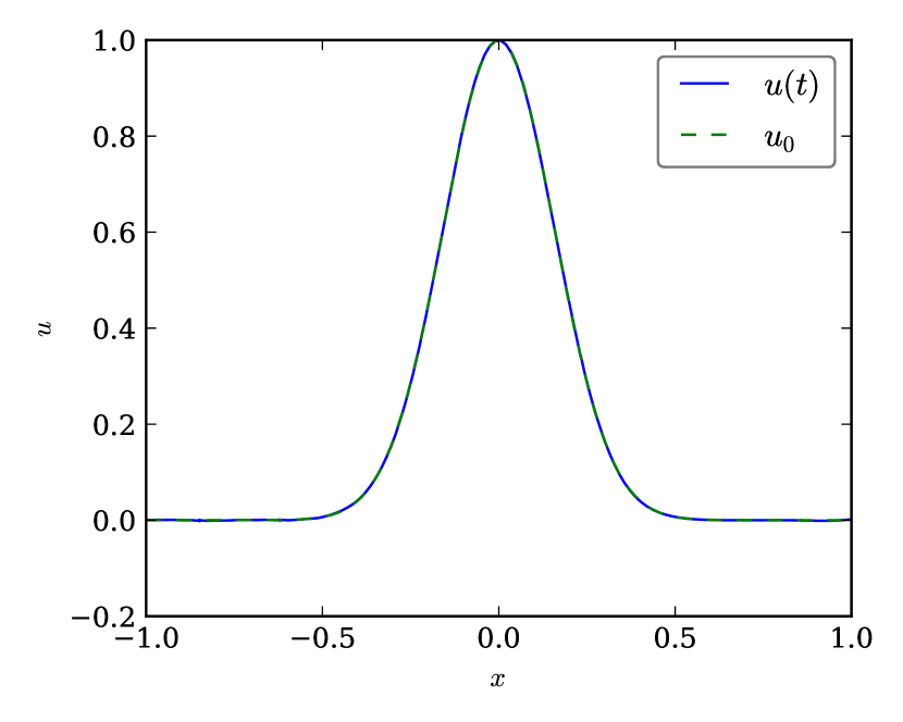
(d) Lobatto-Legendre nodes, $\mat{J}$ as diagonal multiplication matrix.

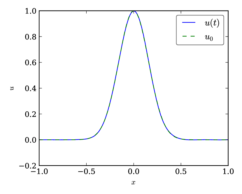
(e) Gauß-Legendre nodes, $\mat{J}$ as diagonal multiplication matrix.

Figure 2: Results of the simulations for linear advection using $5$ elements on grid 3 (geometrically increasing widths) with polynomials of degree $\leq p=9$, the central flux, and the quadratic mapping. Each Figure shows the values of $u(t=4)$ (blue line) and $u(0)=u_{0}$ (green, dashed). (For interpretation of the references to colour in this figure legend, the reader is referred to the web version of this article.)

4.3 Multiple dimensions

In order to apply the methods of the previous sections to multi-dimensional problems, it is common to use tensor product bases and rectangular grids. Only curvilinear coordinates deserve a special treatment in this case, since all other desired properties extend naturally to several space dimensions. However, genuinely multi-dimensional SBP operators can be constructed as well. Here, the extension of the analytical setting of section 3 is described, similarly to the numerical setting of [7], see also [16, section 6].

As in section 3, there is a finite-dimensional (real) Hilbert space $X_{V}$ of functions on the $d$ dimensional reference (volume) element $\Omega$, equipped with a basis $\mathcal{B}_{V}$. With regard to this basis, the scalar product is represented by the mass matrix $\mat{M}$ and approximates the $L^{2}$ norm on $X_{V}$. Moreover, there are $d$ derivative operators $\mat{D_{i}},i\in\mathinner{\left\{1,\dots,d\right\}}$, denoting the partial derivative in the $i$-th coordinate direction.

Furthermore, the functions on the $d-1$ dimensional boundary $\partial\Omega$ are members of the Hilbert space $X_{B}$ with basis $\mathcal{B}_{B}$. The associated scalar product is given by the matrix $\mat{B}$, approximating the $L^{2}$ scalar product via

$$\underline{u_{B}}^{T}\mat{B}\underline{v_{B}}=\left\langle\underline{u_{B}},\underline{v_{B}}\right\rangle_{B}\approx\left\langle u_{B},v_{B}\right\rangle_{L^{2}(\partial\Omega)}=\int_{\partial\Omega}u_{B}v_{B}.$$ (43)

As in one dimension, there is a restriction operator $\mat{R}$ mapping $X_{V}$ to $X_{B}$. Finally, there are $d$ operators $\mat{N_{i}},i\in\mathinner{\left\{1,\dots,d\right\}},$ on $X_{B}$ performing multiplication with the $i$-th component of the outer unit normal $\nu$ at $\partial\Omega$. Together, these operators approximate

$$\underline{u}^{T}\mat{R}[^{T}]\mat{B}\mat{N_{i}}\mat{R}\underline{v}\approx\int_{\partial\Omega}uv\,\nu_{i}.$$ (44)

In the end, the SBP property in multiple dimensions can be formulated as

$$\mat{M}\mat{D_{i}}+\mat{D_{i}}[^{T}]\mat{M}=\mat{R}[^{T}]\mat{B}\mat{N_{i}}\mat{R},$$ (45)

mimicking the divergence theorem

$$\int_{\Omega}u(\partial_{i}v)+\int_{\Omega}(\partial_{i}u)v\approx\underline{u}^{T}\mat{M}\mat{D_{i}}\underline{v}+\underline{u}^{T}\mat{D_{i}}[^{T}]\mat{M}\underline{v}=\underline{u}^{T}\mat{R}[^{T}]\mat{B}\mat{N_{i}}\mat{R}\underline{v}\approx\int_{\partial\Omega}uv\,\nu_{i}.$$ (46)

Of course, tensor product bases formed by one-dimensional SBP bases fulfil the requirements for multi-dimensional SBP bases.

Remark 7.

For curvilinear grids in multiple dimensions, the metric identities are crucial for free stream preservation, conservation and stability, as described inter alia in [11]. An application using split-form discontinuous Galerkin methods for the shallow water equations in two-dimensions on curvilinear grids is presented in [27].

5 Summary and discussion

In this work, an extended analytical framework for SBP methods has been proposed. Using the results of [19], the linearly stable CPR methods of [24, 25] and the DGSEM of [4] are embedded in this framework.

Additionally, new forms of correction terms for nonlinear conservation laws are developed, using the inviscid Burgers’ equation as an example. These correction terms for both divergence and restriction to the boundary extend the skew-symmetric form of conservation laws used in traditional FD SBP methods and the DGSEM based on Lobatto nodes [3, 4].

For the first time, these new corrections allow for both modal and nodal SBP bases without any further conditions on the norm (e.g. diagonal) or the presence of nodes at the boundary. Using the SBP property, both conservation and stability in a discrete norm adapted to the chosen bases are proved. These results extend directly to traditional SBP methods lacking the foundation of an analytical basis, since only structural properties of the representations in a given basis are used.

Moreover, stability for curvilinear grids and dense norms is obtained by using a suitable way to compute the Jacobian. Thus, complications that have been known in the FD framework of SBP methods can be circumvented for SBP CPR methods.

A straightforward extension of the analytical setting to multiple dimensions is described in [16]. Similar to the numerical setting of [1, 7], this genuinely multi-dimensional formulation allows inter alia simplex elements and does not rely on a tensor product extension. Of course, the standard multi-dimensional setting using tensor products is embedded therein.

Further research includes fully discrete schemes and other examples for nonlinear systems of conservation laws.

Appendix A Some bases

The analytical setting described in section 3.1 uses finite dimensional Hilbert spaces to represent numerical solutions. In all cases considered in this article, the space of polynomials of degree $\leq p$ has been used. However, for concrete computations, a basis has to be selected. If the derivative $\mat{D}$, restriction $\mat{R}$, and mass matrix $\mat{M}$ are exact for polynomials of degree $\leq p$, the SBP property (2) is fulfilled, since integration by parts can be applied, see also [13, 8]:

$$\underline{u}^{T}\mat{M}\mat{D}\underline{v}+\underline{u}^{T}\mat{D}[^{T}]\mat{M}\underline{v}=\int_{-1}^{1}u\,(\partial_{x}v)\operatorname{d\!}x+\int_{-1}^{1}(\partial_{x}u)\,v\operatorname{d\!}x=\mathinner{u\,v\Bigr{\rvert}}_{-1}^{1}=\underline{u}^{T}\mat{R}[^{T}]\mat{B}\mat{R}\underline{v}.$$

Furthermore, the matrix representations of linear operators ($\mat{R},\mat{D}$) and bilinear forms ($\mat{M}$) can be computed in one basis and then transformed via the standard transformation rules to another basis (at least in theory and for small polynomial degrees, since the condition numbers might increase drastically for higher polynomial degrees).

To compute the matrices $\mat{M},\mat{D}$ for the nodal bases using Chebyshev points, the associated matrices in a modal Legendre basis are used. The coordinate transformation from a nodal basis with nodes $\xi_{0},\dots,\xi_{p}$ to a modal basis of Legendre polynomials $\phi_{0},\dots,\phi_{p}$ of degree $\leq p$ is given by the Vandermonde matrix $\mat{V}$ with $V_{i,j}=\phi_{j}(\xi_{i})$. Writing vectors and matrices with regard to the modal basis with $\hat{\cdot}$, the transformation is $\mat{V}\underline{\hat{u}}=\underline{u}$. Thus, operators like the derivative are transformed as $\mat{\hat{D}}=\mat{V}[^{-1}]\mat{D}\mat{V}$ and matrices associated with a scalar product like $\mat{M}$ as $\mat{\hat{M}}=\mat{V}[^{T}]\mat{M}\mat{V}$.

The modal matrices are

$$\mat{\hat{M}}=\begin{pmatrix}2\\ &\frac{2}{3}\\ &&\ddots\\ &&&\frac{2}{2p+1}\end{pmatrix},\quad\mat{\hat{D}}=\begin{pmatrix}0&1&0&1&0&\dots\\ 0&0&3&0&3&\dots\\ 0&0&0&5&0&\dots\\ 0&0&0&0&7&\dots\\ \vdots&\vdots&\vdots&\vdots&\vdots&\ddots\end{pmatrix}.$$ (47)

Using $p=2$ as an example, the nodal bases with dense norm are given by the following matrices.

• The roots of the Chebyshev polynomials of first kind are $\xi_{i}=\cos\left(\frac{2i+1}{2p+2}\pi\right)$, for $i\in\mathinner{\left\{p,p-1,\dots,0\right\}}$. The Vandermonde matrix is

  $$\mat{V}=\begin{pmatrix}1&-\frac{\sqrt{3}}{2}&\frac{5}{8}\\ 1&0&-\frac{1}{2}\\ 1&\frac{\sqrt{3}}{2}&\frac{5}{8}\\ \end{pmatrix}.$$ (48)

  Calculating the mass matrix as $\mat{M}=\mat{V}^{-T}\mat{\hat{M}}\mat{V}$ results in

  $$\mat{M}=\begin{pmatrix}\frac{2}{5}&\frac{4}{45}&-\frac{2}{45}\\ \frac{4}{45}&\frac{14}{15}&\frac{4}{45}\\ -\frac{2}{45}&\frac{4}{45}&\frac{2}{5}\\ \end{pmatrix}.$$ (49)

  The restriction (interpolation to the boundary) and boundary matrices used are

  $$\mat{R}=\begin{pmatrix}\frac{2+\sqrt{3}}{3}&-\frac{1}{3}&\frac{2-\sqrt{3}}{3}\\ \frac{2-\sqrt{3}}{3}&-\frac{1}{3}&\frac{2+\sqrt{3}}{3}\\ \end{pmatrix},\quad\mat{B}=\begin{pmatrix}-1&0\\ 0&1\\ \end{pmatrix}.$$ (50)

  Computing the derivative matrix via $\mat{D}=\mat{V}\mat{\hat{D}}\mat{V}^{-1}$ yields

  $$\mat{D}=\begin{pmatrix}-\sqrt{3}&\frac{4\sqrt{3}}{3}&-\frac{\sqrt{3}}{3}\\ -\frac{\sqrt{3}}{3}&0&\frac{\sqrt{3}}{3}\\ \frac{\sqrt{3}}{3}&-\frac{4\sqrt{3}}{3}&\sqrt{3}\\ \end{pmatrix}.$$ (51)

• The extrema of the Chebyshev polynomials of first kind are $\xi_{i}=\cos\left(\frac{i}{p}\pi\right)$, for $i\in\mathinner{\left\{p,p-1,\dots,0\right\}}$. Thus, the matrices are

  $$\mat{V}=\begin{pmatrix}1&-1&1\\ 1&0&-\frac{1}{2}\\ 1&1&1\end{pmatrix},\quad\mat{M}=\begin{pmatrix}\frac{4}{15}&\frac{2}{15}&-\frac{1}{15}\\ \frac{2}{15}&\frac{16}{15}&\frac{2}{15}\\ -\frac{1}{15}&\frac{2}{15}&\frac{4}{15}\end{pmatrix},\quad\mat{R}=\begin{pmatrix}1&0&0\\ 0&0&1\end{pmatrix},\quad\mat{D}=\begin{pmatrix}-\frac{3}{2}&2&-\frac{1}{2}\\ -\frac{1}{2}&0&\frac{1}{2}\\ \frac{1}{2}&-2&\frac{3}{3}\end{pmatrix}.$$ (52)

• Finally, the roots of the Chebyshev polynomials of second kind are $\xi_{i}=\cos\left(\frac{i+1}{p+2}\pi\right)$, where again $i\in\mathinner{\left\{p,p-1,\dots,0\right\}}$. Therefore, the matrices are

  $$\mat{V}=\begin{pmatrix}1&-\frac{\sqrt{2}}{2}&\frac{1}{4}\\ 1&0&-\frac{1}{2}\\ 1&\frac{\sqrt{2}}{2}&\frac{1}{4}\end{pmatrix},\quad\mat{M}=\begin{pmatrix}\frac{11}{15}&-\frac{2}{15}&\frac{1}{15}\\ -\frac{2}{15}&\frac{14}{15}&-\frac{2}{15}\\ \frac{1}{15}&-\frac{2}{15}&\frac{11}{15}\end{pmatrix},$$ (53)

  $$\mat{R}=\begin{pmatrix}\frac{2+\sqrt{2}}{2}&-1&\frac{2-\sqrt{2}}{2}\\ \frac{2-\sqrt{2}}{2}&-1&\frac{2+\sqrt{2}}{2}\end{pmatrix},\quad\mat{D}=\begin{pmatrix}-\frac{3\sqrt{2}}{2}&2\sqrt{2}&-\frac{\sqrt{2}}{2}\\ -\frac{\sqrt{2}}{2}&0&\frac{\sqrt{2}}{2}\\ \frac{\sqrt{2}}{2}&-2\sqrt{2}&\frac{3\sqrt{2}}{2}\end{pmatrix}.$$ (54)

Additionally, the diagonal-norm nodal bases are

• Gauß-Legendre basis with matrices

  $$\mat{M}=\begin{pmatrix}\frac{5}{9}&0&0\\ 0&\frac{8}{9}&0\\ 0&0&\frac{5}{9}\\ \end{pmatrix},\quad\mat{R}=\begin{pmatrix}\frac{5+\sqrt{15}}{6}&-\frac{2}{3}&\frac{5-\sqrt{15}}{6}\\ \frac{5-\sqrt{15}}{6}&-\frac{2}{3}&\frac{5+\sqrt{15}}{6}\end{pmatrix},\quad\mat{D}=\begin{pmatrix}-\frac{\sqrt{15}}{2}&\frac{2\sqrt{15}}{3}&-\frac{\sqrt{15}}{6}\\ -\frac{\sqrt{15}}{6}&0&\frac{\sqrt{15}}{6}\\ \frac{\sqrt{15}}{6}&-\frac{2\sqrt{15}}{3}&\frac{\sqrt{15}}{2}\end{pmatrix}.$$ (55)

• Lobatto-Legendre basis with matrices

  $$\mat{M}=\begin{pmatrix}\frac{1}{3}&0&0\\ 0&\frac{4}{3}&0\\ 0&0&\frac{1}{3}\end{pmatrix},\quad\mat{R}=\begin{pmatrix}1&0&0\\ 0&0&1\end{pmatrix},\quad\mat{D}=\begin{pmatrix}-\frac{3}{2}&2&-\frac{1}{2}\\ -\frac{1}{2}&0&\frac{1}{2}\\ \frac{1}{2}&-2&\frac{3}{2}\\ \end{pmatrix}.$$ (56)

Appendix B Numerical solutions for Burgers’ equation

Here, the numerical solutions corresponding to the energy and momentum in Figure 1 of section 3.3 are shown. The values of $u(3)$ are in general similar – two approximately affine-linear parts and a discontinuous part with oscillations around $x=1$. Despite of this, the intensity of oscillations depends on the bases and associated projection used for multiplication.

In this case, the Gauß-Legendre nodes and modal Legendre polynomials seem to be visually indistinguishable. Contrary, the computations using a nodal basis are much more efficient, since only simple multiplication of nodal values has to be performed.

References

- Fernández et al. [2014a] D.C.D.R. Fernández, P.D. Boom, D.W. Zingg, A generalized framework for nodal first derivative summation-by-parts operators, Journal of Computational Physics 266 (2014a) 214–239.
- Fernández et al. [2014b] D.C.D.R. Fernández, J.E. Hicken, D.W. Zingg, Review of summation-by-parts operators with simultaneous approximation terms for the numerical solution of partial differential equations, Computers & Fluids 95 (2014b) 171–196.
- Fisher et al. [2013] T.C. Fisher, M.H. Carpenter, J. Nordström, N.K. Yamaleev, C. Swanson, Discretely conservative finite-difference formulations for nonlinear conservation laws in split form: Theory and boundary conditions, Journal of Computational Physics 234 (2013) 353–375.
- Gassner [2013] G.J. Gassner, A skew-symmetric discontinuous Galerkin spectral element discretization and its relation to SBP-SAT finite difference methods, SIAM Journal on Scientific Computing 35 (2013) A1233–A1253.
- Gassner et al. [2016] G.J. Gassner, A.R. Winters, D.A. Kopriva, A well balanced and entropy conservative discontinuous Galerkin spectral element method for the shallow water equations, Applied Mathematics and Computation 272 (2016) 291–308.
- Glaubitz et al. [2016] J. Glaubitz, H. Ranocha, P. Öffner, T. Sonar, Enhancing stability of correction procedure via reconstruction using summation-by-parts operators II: Modal filtering, 2016. arXiv:1606.01056, submitted.
- Hicken et al. [2016] J.E. Hicken, D.C.D.R. Fernández, D.W. Zingg, Multidimensional summation-by-parts operators: General theory and application to simplex elements, SIAM Journal on Scientific Computing 38 (2016) A1935--A1958.
- Hicken and Zingg [2013] J.E. Hicken, D.W. Zingg, Summation-by-parts operators and high-order quadrature, Journal of Computational and Applied Mathematics 237 (2013) 111--125.
- Huynh [2007] H. Huynh, A flux reconstruction approach to high-order schemes including discontinuous Galerkin methods, AIAA paper 4079 (2007) 2007.
- Huynh et al. [2014] H. Huynh, Z.J. Wang, P.E. Vincent, High-order methods for computational fluid dynamics: A brief review of compact differential formulations on unstructured grids, Computers & Fluids 98 (2014) 209--220.
- Kopriva [2006] D.A. Kopriva, Metric identities and the discontinuous spectral element method on curvilinear meshes, Journal of Scientific Computing 26 (2006) 301--327.
- Kopriva [2009] D.A. Kopriva, Implementing spectral methods for partial differential equations: Algorithms for scientists and engineers, Springer Science & Business Media, 2009.
- Kopriva and Gassner [2010] D.A. Kopriva, G.J. Gassner, On the quadrature and weak form choices in collocation type discontinuous Galerkin spectral element methods, Journal of Scientific Computing 44 (2010) 136--155.
- Ortleb [2016a] S. Ortleb, Kinetic energy preserving DG schemes based on summation-by-parts operators on interior node distributions, Talk presented at the joint annual meeting of DMV and GAMM, 2016a.
- Ortleb [2016b] S. Ortleb, Kinetic energy preserving DG schemes based on summation-by-parts operators on interior node distributions, PAMM 16 (2016b) 857--858.
- Ranocha [2016] H. Ranocha, SBP operators for CPR methods, Master’s thesis, TU Braunschweig, 2016.
- Ranocha [2017] H. Ranocha, Shallow water equations: Split-form, entropy stable, well-balanced, and positivity preserving numerical methods, GEM -- International Journal on Geomathematics 8 (2017) 85--133. doi:10.1007/s13137-016-0089-9. arXiv:1609.08029.
- Ranocha et al. [2016a] H. Ranocha, J. Glaubitz, P. Öffner, T. Sonar, Enhancing stability of correction procedure via reconstruction using summation-by-parts operators I: Artificial dissipation, 2016a. arXiv:1606.00995, submitted.
- Ranocha et al. [2016b] H. Ranocha, P. Öffner, T. Sonar, Summation-by-parts operators for correction procedure via reconstruction, Journal of Computational Physics 311 (2016b) 299--328. doi:10.1016/j.jcp.2016.02.009. arXiv:1511.02052.
- Svärd [2004] M. Svärd, On coordinate transformations for summation-by-parts operators, Journal of Scientific Computing 20 (2004) 29--42.
- Svärd and Nordström [2014] M. Svärd, J. Nordström, Review of summation-by-parts schemes for initial--boundary-value problems, Journal of Computational Physics 268 (2014) 17--38.
- Tadmor [1987] E. Tadmor, The numerical viscosity of entropy stable schemes for systems of conservation laws. I, Mathematics of Computation 49 (1987) 91--103.
- Tadmor [2003] E. Tadmor, Entropy stability theory for difference approximations of nonlinear conservation laws and related time-dependent problems, Acta Numerica 12 (2003) 451--512.
- Vincent et al. [2011] P.E. Vincent, P. Castonguay, A. Jameson, A new class of high-order energy stable flux reconstruction schemes, Journal of Scientific Computing 47 (2011) 50--72.
- Vincent et al. [2015] P.E. Vincent, A.M. Farrington, F.D. Witherden, A. Jameson, An extended range of stable-symmetric-conservative flux reconstruction correction functions, Computer Methods in Applied Mechanics and Engineering 296 (2015) 248--272.
- Wang and Gao [2009] Z. Wang, H. Gao, A unifying lifting collocation penalty formulation including the discontinuous Galerkin, spectral volume/difference methods for conservation laws on mixed grids, Journal of Computational Physics 228 (2009) 8161--8186.
- Wintermeyer et al. [2015] N. Wintermeyer, A.R. Winters, G.J. Gassner, D.A. Kopriva, An entropy stable nodal discontinuous Galerkin method for the two dimensional shallow water equations on unstructured curvilinear meshes with discontinuous bathymetry, 2015. arXiv:1509.07096.