Summation-by-parts operators for correction procedure via reconstruction

Abstract

The correction procedure via reconstruction (CPR, formerly known as flux reconstruction) is a framework of high order methods for conservation laws, unifying some discontinuous Galerkin, spectral difference and spectral volume methods. Linearly stable schemes were presented by Vincent et al. (2011, 2015), but proofs of non-linear (entropy) stability in this framework have not been published yet (to the knowledge of the authors). We reformulate CPR methods using summation-by-parts (SBP) operators with simultaneous approximation terms (SATs), a framework popular for finite difference methods, extending the results obtained by Gassner (2013) for a special discontinuous Galerkin spectral element method. This reformulation leads to proofs of conservation and stability in discrete norms associated with the method, recovering the linearly stable CPR schemes of Vincent et al. (2011, 2015). Additionally, extending the skew-symmetric formulation of conservation laws by additional correction terms, entropy stability for Burgers’ equation is proved for general SBP CPR methods not including boundary nodes.

1 Introduction

In the field of computational fluid dynamics (CFD), low-order methods are generally robust and reliable and therefore employed in practical calculations. The main advantage of high-order methods towards low-order ones is the possibility of considerably more accurate solutions with the same computing cost, but unfortunately they are less robust and more complicated. In recent years many researchers focus on this topic. There has been a surge of research activities to improve and refine high-order methods as well as to develop new ones with more favourable properties.

We consider in this paper the correction procedure via reconstruction (CPR) method using summation-by-parts (SBP) operators. The CPR combines the flux reconstruction (FR) approach developed by Huynh [13] and the lifting collocation penalty (LCP) by Wang and Gao [24].

Huynh [13] introduced the FR approach to high-order spectral methods for conservation laws in one space dimension and its extension to multiple dimensions using tensor products in 2007. For the case of one spatial dimension, the ansatz amounts to evaluating the derivative of a discontinuous piecewise polynomial function by using its straightforward derivative estimate together with a correction term. Wang and Gao [24] generalised the FR approach in 2009 to lifting collocation penalty methods on triangular grids. Later, the authors involved in the construction of these methods combined the names in the unifying framework of correction procedure via reconstruction (CPR) methods, see [14]. The CPR creates a framework unifying several high-order methods such as discontinuous Galerkin (DG), spectral difference (SD) and spectral volume (SV) methods. These connections were already pointed out and investigated in more detail in [1, 4, 28].

A linear (von Neumann) stability analysis of FR schemes was carried out already by Huynh [13] and in extended form by Vincent, Castonguay and Jameson [21]. A one-parameter family of linearly stable schemes in one dimension was discovered by the same authors [22] using an energy method and extended in 2015 to multiple-parameter families [23]. Extensions of the one-parameter family to advection-diffusion problems and triangular grids were published by the same groups [2, 3, 25].

The analysis of nonlinear stability for CPR methods is far more complex and not as advanced as in the linear case. First results are available in [16, 26, 27].

The application of summation-by-parts (SBP) operators in the CPR framework supplies a new perspective here.

In the context of finite difference (FD) methods, summation-by-parts operators with simultaneous approximation terms (SATs) provide a suitable way to derive stable schemes in a multi-block fashion enforcing boundary conditions in a weak way. They enable the imitation of manipulations of the continuous problem for the discrete method and are thus able to translate results like well-posedness to its discrete counterpart stability. Review articles from Svärd and Nordström [19] and Del Rey Fernández, Hicken, and Zingg [6] provide an insight in the development over the last decades and recent results. There is a strong connection of SBP operators with both skew-symmetric formulations of conservation laws as a means to prove conservation and stability [7], and quadrature rules [12]. Recently, Gassner et al. applied the SBP SAT framework to a particular discontinuous Galerkin spectral element method (DGSEM) to prove stability and discrete conservation for different systems of conservation laws, see inter alia [8, 9, 18, 11]. Another extension of SBP operators has been presented by Del Rey Fernández et al. [5], based on a numerical setting and allowing general operators, connected with quadrature rules.

Here, we use the SBP framework in the general CPR setting. We are able to demonstrate all well-known properties, which have already been proven, but we can further extend the CPR method and show conservation and stability in a nonlinear case, see section 4.

The paper is organised as follows. The SBP and CPR frameworks will be briefly explained in section 2. In the next section, we apply SBP operators in CPR methods and revisit the results of Vincent et al. [22, 23] for constant velocity linear advection.

In section 4, we focus on Burgers’ equation and prove both discrete conservation and stability for a skew-symmetric formulation and Lobatto-Legendre nodes, revisiting the results of [8].

Additionally, we suggest a generalisation of the CPR method to get stability for a general SBP basis, extending the skew-symmetric formulation and being both provably stable and conservative. Numerical test cases are used to confirm the theoretical results. Finally, we discuss open problems and give an outlook on future work.

2 Existing formulations for SBP operators and CPR methods

Both finite difference (FD) SBP methods and CPR schemes are designed as semidiscretisations of hyperbolic conservation laws

$$\partial_{t}u+\partial_{x}f(u)=0,$$ (1)

equipped with appropriate initial and boundary conditions.

2.1 SBP schemes

Traditionally, SBP operators are used in the FD framework. In one space dimension, a set of nodes including both boundary points of the element are used to represent the solution values. Extensions to multiple dimensions are performed via tensor products. To compute the semidiscretisation of (1), $f(u)$ is evaluated at each node and a difference operator is applied. The notation using vectors $\underline{u}$ for the solution values and the differentiation matrix $\underline{\underline{D}}\,$ is very common and results in a finite difference approximation $\underline{\underline{D}}\,\underline{f}$ of $\partial_{x}f$.

In order to be an SBP operator, the derivative matrix needs to be written as $D=P^{-1}Q$, $Q+Q^{T}=B=\operatorname{diag}(-1,0,\dots,0,1)$, where $P$ is a symmetric and positive definite matrix with associated norm $\mathinner{\!\left\lVert\underline{u}\right\rVert}^{2}_{P}=\underline{u}^{T}\underline{\underline{P}}\,\underline{u}$, approximating the $L^{2}$ norm, see inter alia the review [19] and references cited therein. Boundary (both of the computational domain and between blocks) conditions are imposed weakly, using a simultaneous-approximation-term (SAT) formulation (see inter alia [7]), involving differences of desired and given values at boundary points. Thus, the SBP CPR methods described in the next chapter extend these schemes.

2.2 CPR methods

The FR approach in one space dimension described by Huynh [13] uses a nodal polynomial basis of order $p$ in the standard element $[-1,1]$. All elements are mapped to this standard element and the computations are performed there. Extensions to multiple dimensions are performed via tensor products. The semidiscretisation of (1) (i.e. the computation of $\partial_{x}f(u)$) consists of the following steps, see also the review [14] and references cited therein:

• Interpolate the solution to the cell boundaries at $-1$ and $1$ (if these values are not already given as coefficients of the nodal basis).

• Compute common numerical fluxes $f^{num}$ at each cell boundary.

• Compute the flux $f(u)$ pointwise in each node.

• Interpolate the flux $f(u)$ to the boundary and add polynomial correction functions $g_{L}$, $g_{R}$ of degree $p+1$, multiplied by the difference of $f_{L/R}-f^{num}_{L/R}$ of the flux and the numerical flux at the corresponding boundary.

• Finally, compute the resulting derivative of $f+(f_{L}-f^{num}_{L})g_{L}+(f_{R}-f^{num}_{R})g_{R}$, using exact differentiation for the polynomial basis.

Wang and Gao [24, equation (3.14)] formulated the lifting collocation penalty (LCP) approach for the semidiscretisation of (1) on triangles as the exact derivative of the flux $f(u)$ computed as above by pointwise evaluation at the nodes plus additional correction terms in the form of a linear combination of the differences between a common numerical flux and the flux $f$ at points on the boundary of the cell.

Since the approaches are similar and can be reformulated in the other way, the common name correction procedure via reconstruction (CPR) was used for both schemes. In the next section, the involved linear combination of penalty terms at the boundary is rewritten in another way, allowing more abstractions and compact formulations.

3 CPR methods using SBP operators: Linear advection

This chapter focuses on a new formulation of CPR methods with special attention paid to SBP operators. Additionally, constant velocity linear advection is used as a test case to investigate linear stability and conservation properties of the schemes.

3.1 The one dimensional setting

After mapping each element to the standard element $[-1,1]$, a CPR method can be formulated as

$$\partial_{t}\underline{u}+\underline{\underline{D}}\,\underline{f}+\underline{\underline{C}}\,(\underline{f}^{num}-\underline{\underline{R}}\,\underline{f})=0.$$ (2)

Here, $\underline{u},\underline{f}$ are the finite dimensional representation of $u$, $f(u)$ in the standard element and $\underline{f}^{num}$ is the representation of the numerical flux on the boundary. The linear operators representing differentiation and restriction (interpolation) to the boundary of the standard element are represented via the matrices $\underline{\underline{D}}\,$ and $\underline{\underline{R}}\,$, respectively. Other parameters of the correction operator are encoded in the correction matrix $\underline{\underline{C}}\,$. Thus, for a given standard element, a CPR method is parameterized by

• A basis $\mathcal{B}$ for the local expansion, determining the derivative and restriction (interpolation) matrices $\underline{\underline{D}}\,$ and $\underline{\underline{R}}\,$.

• A correction matrix $\underline{\underline{C}}\,$, adapted to the chosen basis.

For the representation of an SBP operator, the basis $\mathcal{B}$ has to be associated with a (volume) quadrature rule, given by nodes $z_{0},\dots,z_{p}$ and appropriate positive weights $\omega_{0},\dots,\omega_{p}$. The values of $u$ at the nodes are the coefficients of the local expansion, i.e. $\underline{u}=(u(z_{0}),\dots,u(z_{p}))^{T}$. The quadrature weights determine a positive definite Matrix $\underline{\underline{M}}\,=\operatorname{diag}(\omega_{0},\dots,\omega_{p})$ associated with a (discrete) norm $\mathinner{\!\left\lVert u\right\rVert}_{M}^{2}=\underline{u}^{T}\underline{\underline{M}}\,\underline{u}$. Besides the volume quadrature rule, there must be a quadrature rule for the boundary, approximating the outward flux through the boundary as in the divergence theorem. In the present one dimensional setting, this quadrature rule is simply given by exact evaluation at the endpoints $\mathinner{\cdot\rvert}_{-1}^{1}$. The basis and it’s associated quadrature rules must satisfy the SBP property

$$\underline{\underline{M}}\,\underline{\underline{D}}\,+\underline{\underline{D}}\,^{T}\underline{\underline{M}}\,=\underline{\underline{R}}\,^{T}\underline{\underline{B}}\,\underline{\underline{R}}\,,$$ (3)

in order to mimic integration by parts on a discrete level

$$\underline{u}^{T}\underline{\underline{M}}\,\underline{\underline{D}}\,\underline{v}+(\underline{\underline{D}}\,\underline{u})^{T}\underline{\underline{M}}\,\underline{v}$$ (4)

$$\approx\int_{-1}^{1}u\,\partial_{x}v\operatorname{d\!}x+\int_{-1}^{1}\partial_{x}u\,v\operatorname{d\!}x=\mathinner{u\,v\Bigr{\rvert}}_{-1}^{1}$$

$$\approx(\underline{\underline{R}}\,\underline{u})^{T}\underline{\underline{B}}\,(\underline{\underline{R}}\,\underline{u}).$$

As an example, consider Gauß-Lobatto-Legendre integration with its associated basis of point values at Lobatto nodes in $(-1,1)$. Then, the restriction and boundary integral matrices reduce to

$$\underline{\underline{R}}\,=\begin{pmatrix}1&0&\dots&0\\ 0&\dots&0&1\end{pmatrix},\quad\underline{\underline{B}}\,=\begin{pmatrix}-1&0\\ 0&1\end{pmatrix}.$$ (5)

Using the special choice $\underline{\underline{C}}\,=\underline{\underline{M}}\,^{-1}\underline{\underline{R}}\,^{T}\underline{\underline{B}}\,$ and defining $\underline{\underline{\widetilde{B}}}\,\mathrel{\mathop{\ordinarycolon}}=\underline{\underline{R}}\,^{T}\underline{\underline{B}}\,\underline{\underline{R}}\,$, i.e. $\underline{\underline{\widetilde{B}}}\,=\operatorname{diag}(-1,0,\dots,0,1)$, the CPR method of equation (2) reduces to

$$\partial_{t}\underline{u}+\underline{\underline{D}}\,\underline{f}+\underline{\underline{M}}\,^{-1}\underline{\underline{\widetilde{B}}}\,(\underline{\widetilde{f}}^{num}-\underline{f})=0,$$ (6)

where $\underline{\widetilde{f}}^{num}=(f^{num}_{L},0,\dots,0,f^{num}_{R})$ contains the numerical flux at the left and right boundary and satisfies $\underline{f}^{num}=\underline{\underline{R}}\,\underline{\widetilde{f}}^{num}$. Equation (6) is the strong form of the DGSEM formulation of Gassner [8], which he proved to be a diagonal norm SBP operator.

3.2 Conservation

Consider now a CPR method given by a nodal basis of polynomials of degree $\leq p$ and an associated (symmetric) quadrature rule that is exact for polynomials of degree $\leq 2p-1$, for example Gauß-Legendre or Gauß-Lobatto-Legendre quadrature. Then, due to exact integration of polynomials of the form $u\,\partial_{x}v$, where $u,v$ are polynomials of degree $\leq p$, the SBP property (3) automatically holds, see also [17]. Let $\underline{1}$ denote the representation of the constant function $x\mapsto 1$ in the chosen basis, i. e. $\underline{1}=(1,\dots,1)^{T}$ for a nodal polynomial basis.

In order to investigate conservation properties in the continuous setting, the function $u$ is multiplied with the constant function $x\mapsto 1$ and integrated over the interval $(a,b)$, resulting in

$$\dfrac{\operatorname{d\!}{}}{\operatorname{d\!}{t}}\int_{a}^{b}u\operatorname{d\!}x=-\int_{a}^{b}\partial_{x}f(u)\operatorname{d\!}x=\mathinner{f(u)\Bigr{\rvert}}_{a}^{b}=f_{R}-f_{L}.$$ (7)

Mimicking this derivation in the semidiscrete setting (in the standard element) leads to

$$\dfrac{\operatorname{d\!}{}}{\operatorname{d\!}{t}}\int_{-1}^{1}u\operatorname{d\!}x=\dfrac{\operatorname{d\!}{}}{\operatorname{d\!}{t}}\underline{1}^{T}\underline{\underline{M}}\,\underline{u}=-\underline{1}^{T}\underline{\underline{M}}\,\left(\underline{\underline{D}}\,\underline{f}+\underline{\underline{C}}\,(\underline{f}^{num}-\underline{\underline{R}}\,\underline{f})\right).$$ (8)

Using the SBP property (3) results in

$$\dfrac{\operatorname{d\!}{}}{\operatorname{d\!}{t}}\underline{1}^{T}\underline{\underline{M}}\,\underline{u}=\underline{1}^{T}\underline{\underline{D}}\,^{T}\underline{\underline{M}}\,\underline{f}-\underline{1}^{T}\underline{\underline{R}}\,^{T}\underline{\underline{B}}\,\underline{\underline{R}}\,\underline{f}-\underline{1}^{T}\underline{\underline{M}}\,\underline{\underline{C}}\,(\underline{f}^{num}-\underline{\underline{R}}\,\underline{f}).$$ (9)

Since discrete differentiation is exact for polynomials of degree $\leq p$ and especially for constant functions, $\underline{\underline{D}}\,\underline{1}=0$, we get

$$\dfrac{\operatorname{d\!}{}}{\operatorname{d\!}{t}}\underline{1}^{T}\underline{\underline{M}}\,\underline{u}=-(\underline{1}^{T}\underline{\underline{R}}\,^{T}\underline{\underline{B}}\,-\underline{1}^{T}\underline{\underline{M}}\,\underline{\underline{C}}\,)\underline{\underline{R}}\,\underline{f}-\underline{1}^{T}\underline{\underline{M}}\,\underline{\underline{C}}\,\underline{f}^{num}.$$ (10)

Lemma 1.

If the assumptions of this subsection are complied with and the correction operator of the CPR method satisfies $\underline{1}^{T}\underline{\underline{M}}\,\underline{\underline{C}}\,=\underline{1}^{T}\underline{\underline{R}}\,^{T}\underline{\underline{B}}\,$, then the scheme is conservative (across elements).

Proof.

Inserting the condition into (10) gives

$$\dfrac{\operatorname{d\!}{}}{\operatorname{d\!}{t}}\underline{1}^{T}\underline{\underline{M}}\,\underline{u}=-\underline{1}^{T}\underline{\underline{R}}\,^{T}\underline{\underline{B}}\,\underline{f}^{num}=f^{num}_{R}-f^{num}_{L},$$ (11)

due to exact evaluation of the boundary integral for polynomials of degree $\leq p$. Summing up the contributions of all elements and bearing in mind that the numerical flux at the boundary point between two adjacent elements is the same for both, biased only by a factor of $-1$ for one element but not for the other, results in the global equality

$$\dfrac{\operatorname{d\!}{}}{\operatorname{d\!}{t}}\int_{a}^{b}u\operatorname{d\!}x=\underline{1}^{T}\underline{\underline{M}}\,\underline{u}=f_{R}-f_{L}$$ (12)

also for the numerical scheme. ∎

Assuming periodic boundary conditions therefore leads to global conservation

$$\dfrac{\operatorname{d\!}{}}{\operatorname{d\!}{t}}\int_{a}^{b}u\operatorname{d\!}x=\dfrac{\operatorname{d\!}{}}{\operatorname{d\!}{t}}\underline{1}^{T}\underline{\underline{M}}\,\underline{u}=0.$$ (13)

Lemma 1 proofs conservation across elements. On a sub-element level, conservation for diagonal-norm SBP operators (including boundary nodes) has been proven in [7] in the context of the Lax-Wendroff theorem.

3.3 Linear stability

Specializing on a certain type of flux, namely the flux of linear advection with constant velocity $1$, the conservation law reduces to

$$\partial_{t}u+\partial_{x}u=0.$$ (14)

In the continuous setting, proving stability with respect to the $L^{2}$ norm is simply an application of integration by parts. Multiplying equation (14) by the solution $u$ and integrating over the domain leads to

$$\int u\,\partial_{t}u=-\int u\,\partial_{x}u=-\mathinner{\frac{1}{2}u^{2}\Bigr{\rvert}}+\int\partial_{x}u\,u.$$ (15)

Summing up the first and the last equality results in

$$\dfrac{\operatorname{d\!}{}}{\operatorname{d\!}{t}}\mathinner{\!\left\lVert u\right\rVert}_{L^{2}}^{2}=-\mathinner{\frac{1}{2}u^{2}\Bigr{\rvert}},$$ (16)

allowing an estimate of the solution’s norm in terms of the initial and boundary conditions, i.e. well-posedness. Assuming compact support or periodic boundary conditions simplifies the estimate to $\dfrac{\operatorname{d\!}{}}{\operatorname{d\!}{t}}\mathinner{\!\left\lVert u\right\rVert}_{L^{2}}^{2}=0$.

Mimicking this manipulations in the discrete setting of an SBP CPR method reads as

$$\int u\,\partial_{t}u\approx\underline{u}^{T}\underline{\underline{M}}\,\dfrac{\operatorname{d\!}{}}{\operatorname{d\!}{t}}\underline{u}=-\underline{u}^{T}\underline{\underline{M}}\,\left(\underline{\underline{D}}\,\underline{u}+\underline{\underline{C}}\,(\underline{f}^{num}-\underline{\underline{R}}\,\underline{u})\right).$$ (17)

Applying the SBP property (3) as in the previous section results in

$$\underline{u}^{T}\underline{\underline{M}}\,\dfrac{\operatorname{d\!}{}}{\operatorname{d\!}{t}}\underline{u}=\underline{u}^{T}\underline{\underline{D}}\,^{T}\underline{\underline{M}}\,\underline{u}-\underline{u}^{T}\underline{\underline{R}}\,^{T}\underline{\underline{B}}\,\underline{\underline{R}}\,\underline{u}-\underline{u}^{T}\underline{\underline{M}}\,\underline{\underline{C}}\,(\underline{f}^{num}-\underline{\underline{R}}\,\underline{u}).$$ (18)

Summing up these equations and using the symmetry of the scalar product induced by $\underline{\underline{M}}\,$ yields

$$\dfrac{\operatorname{d\!}{}}{\operatorname{d\!}{t}}\mathinner{\!\left\lVert u\right\rVert}_{M}^{2}=-\underline{u}^{T}\underline{\underline{R}}\,^{T}\underline{\underline{B}}\,\underline{\underline{R}}\,\underline{u}-2\underline{u}^{T}\underline{\underline{M}}\,\underline{\underline{C}}\,(\underline{f}^{num}-\underline{\underline{R}}\,\underline{u}).$$ (19)

Assuming now the special form $\underline{\underline{C}}\,=\underline{\underline{M}}\,^{-1}\underline{\underline{R}}\,^{T}\underline{\underline{B}}\,$ simplifies the last equation to

$$\dfrac{\operatorname{d\!}{}}{\operatorname{d\!}{t}}\mathinner{\!\left\lVert u\right\rVert}_{M}^{2} =\underline{u}^{T}\underline{\underline{R}}\,^{T}\underline{\underline{B}}\,\underline{\underline{R}}\,\underline{u}-2\underline{u}^{T}\underline{\underline{R}}\,^{T}\underline{\underline{B}}\,\underline{f}^{num}$$ (20)

$$=\underline{u}^{T}\underline{\underline{R}}\,^{T}\underline{\underline{B}}\,(\underline{\underline{R}}\,\underline{u}-2\underline{f}^{num}).$$

Due to exact evaluation of the boundary terms for $\underline{u}$, representing a polynomial of degree $\leq p$, this can be written as

$$\dfrac{\operatorname{d\!}{}}{\operatorname{d\!}{t}}\mathinner{\!\left\lVert u\right\rVert}_{M}^{2}=u_{R}(u_{R}-2f^{num}_{R})-u_{L}(u_{L}-2f^{num}_{L}),$$ (21)

where the indices $R$ and $L$ indicate values at the right and left boundary, respectively. Therefore, a similar estimate of the norm of the numerical solution in terms of boundary data and the numerical flux is possible. Assuming again periodic boundary conditions or compact support reduces the global rate of change to a sum of local contributions of the form $u_{-}(u_{-}-2f^{num})-u_{+}(u_{+}-2f^{num})$, where $f^{num}$ is the common numerical flux and $u_{-}$ is the value $u_{R}$ on the right boundary of the left element and $u_{+}$ is appropriately defined. Using a standard numerical flux of the form

$$f^{num}(u_{-},u_{+})=\frac{u_{+}+u_{-}}{2}-\alpha(u_{+}-u_{-}),$$ (22)

recovering a central scheme for $\alpha=0$ and a fully upwind scheme for $\alpha=1$, yields

$$u_{-}(u_{-}-2f^{num})-u_{+}(u_{+}-2f^{num})$$ (23)

$$=u_{-}^{2}-u_{+}^{2}-u_{-}(u_{-}+u_{+})+2\alpha u_{-}(u_{+}-u_{-})$$

$$\quad+u_{+}(u_{-}+u_{+})-2\alpha u_{+}(u_{+}-u_{-})$$

$$=-2\alpha(u_{+}-u_{-})^{2}.$$

Thus, $\alpha\geq 0$ ensures $\dfrac{\operatorname{d\!}{}}{\operatorname{d\!}{t}}\mathinner{\!\left\lVert u\right\rVert}_{M}\leq 0$ and therefore stability, the discrete analogue to well-posedness.

The basic idea of Jameson [15] to show linear stability is using the equivalence of norms in finite dimensional vector spaces and showing stability not in a regular $L^{2}$ norm, but a kind of Sobolev norm involving derivatives, as also explained in [1] and used in [22, 23] to derive linearly stable FR methods. Although the ansatz here is very different, some calculations are similar and in the end, the same schemes will be derived. The difference is, that Vincent et al. [23] used continuous integral norms for their derivations whereas this setting uses fully discrete norms adapted to the solution point coordinates. Therefore, they could not recognize any influence of the solution points on the stability properties in the linear case. For the nonlinear case, the influence of these nodes was stressed in [16].

Following these ideas, stability is investigated for a discrete norm given by $\underline{\underline{M}}\,+\underline{\underline{K}}\,$, where $\underline{\underline{M}}\,$ is the matrix associated as usual with the quadrature rule given by the polynomial basis and $\underline{\underline{K}}\,$ is a symmetric matrix satisfying $\underline{\underline{M}}\,+\underline{\underline{K}}\,>0$, i.e. positive definite. Then, the rate of change of the discrete norm $\mathinner{\!\left\lVert u\right\rVert}_{M+K}^{2}=\underline{u}^{T}(\underline{\underline{M}}\,+\underline{\underline{K}}\,)\underline{u}$ can be computed as

$$\underline{u}^{T}(\underline{\underline{M}}\,+\underline{\underline{K}}\,)\dfrac{\operatorname{d\!}{}}{\operatorname{d\!}{t}}\underline{u}=-\underline{u}^{T}(\underline{\underline{M}}\,+\underline{\underline{K}}\,)\left(\underline{\underline{D}}\,\underline{u}+\underline{\underline{C}}\,(\underline{f}^{num}-\underline{\underline{R}}\,\underline{u})\right),$$ (24)

which can also be written as

$$\underline{u}^{T}(\underline{\underline{M}}\,+\underline{\underline{K}}\,)\dfrac{\operatorname{d\!}{}}{\operatorname{d\!}{t}}\underline{u}= -\underline{u}^{T}\underline{\underline{K}}\,\underline{\underline{D}}\,\underline{u}-\underline{u}^{T}(\underline{\underline{M}}\,+\underline{\underline{K}}\,)\underline{\underline{C}}\,(\underline{f}^{num}-\underline{\underline{R}}\,\underline{u})$$ (25)

$$+\underline{u}^{T}\underline{\underline{D}}\,^{T}\underline{\underline{M}}\,\underline{u}-\underline{u}^{T}\underline{\underline{R}}\,^{T}\underline{\underline{B}}\,\underline{\underline{R}}\,\underline{u},$$

due to the SBP property (3). Again, adding the last two equations yields

$$\dfrac{\operatorname{d\!}{}}{\operatorname{d\!}{t}}\mathinner{\!\left\lVert u\right\rVert}_{M+K}^{2}$$ (26)

$$=-2\underline{u}^{T}\underline{\underline{K}}\,\underline{\underline{D}}\,\underline{u}-2\underline{u}^{T}(\underline{\underline{M}}\,+\underline{\underline{K}}\,)\underline{\underline{C}}\,(\underline{f}^{num}-\underline{\underline{R}}\,\underline{u})$$

$$\quad-\underline{u}^{T}\underline{\underline{R}}\,^{T}\underline{\underline{B}}\,\underline{\underline{R}}\,\underline{u}.$$

The last term contains only boundary values and is thus unproblematic. The second term can be rendered as a boundary term by enforcing the correction matrix to be $\underline{\underline{C}}\,=(\underline{\underline{M}}\,+\underline{\underline{K}}\,)^{-1}\underline{\underline{R}}\,^{T}\underline{\underline{B}}\,$, analogously to the previous procedure. Then, the only term remaining to be estimated is the first one.

In the following sections, the multiple parameter family of FR methods of Vincent et al. [23] will be reconsidered using the view of SBP operators. These parameters force the first term to vanish, because $\underline{\underline{K}}\,\underline{\underline{D}}\,$ is chosen to be antisymmetric. Then, using $\underline{\underline{C}}\,=(\underline{\underline{M}}\,+\underline{\underline{K}}\,)^{-1}\underline{\underline{R}}\,^{T}\underline{\underline{B}}\,$, the last equation can be written as

$$\dfrac{\operatorname{d\!}{}}{\operatorname{d\!}{t}}\mathinner{\!\left\lVert u\right\rVert}_{M+K}^{2} =-2\underline{u}^{T}\underline{\underline{R}}\,^{T}\underline{\underline{B}}\,(\underline{f}^{num}-\underline{\underline{R}}\,\underline{u})-\underline{u}^{T}\underline{\underline{R}}\,^{T}\underline{\underline{B}}\,\underline{\underline{R}}\,\underline{u}$$ (27)

$$=\underline{u}^{T}\underline{\underline{R}}\,^{T}\underline{\underline{B}}\,(\underline{\underline{R}}\,\underline{u}-2\underline{f}^{num}),$$

allowing the same estimates as before, leading to linear stability. This proves the following

Lemma 2 (see also [23, Thm.1 ]).

If the SBP CPR method is given by $\underline{\underline{C}}\,=(\underline{\underline{M}}\,+\underline{\underline{K}}\,)^{-1}\underline{\underline{R}}\,^{T}\underline{\underline{B}}\,$, where $\underline{\underline{M}}\,+\underline{\underline{K}}\,$ is positive definite and $\underline{\underline{K}}\,\underline{\underline{D}}\,$ is antisymmetric, then the method is linearly stable in the discrete norm $\mathinner{\!\left\lVert\cdot\right\rVert}_{M+K}$ induced by $\underline{\underline{M}}\,+\underline{\underline{K}}\,$.

3.4 Symmetry

In order to recognize the FR method associated with an SBP CPR method, it suffices to identify the correction matrix $\underline{\underline{C}}\,$ with the derivatives of the left and right correction function $g_{L},g_{R}$. Using again a nodal polynomial basis with symmetric nodes $\xi_{0},\dots,\xi_{p}$ in the standard element, writing

$$\underline{\underline{C}}\,=\begin{pmatrix}g_{L}^{\prime}(\xi_{0})&g_{R}^{\prime}(\xi_{0})\\ \vdots&\vdots\\ g_{L}^{\prime}(\xi_{p})&g_{R}^{\prime}(\xi_{p})\end{pmatrix}$$ (28)

provides the required identification of SBP CPR parameters and FR correction functions. Note that $g_{L}(-1)=1=g_{R}(1)$ is required, so that the integration constant is fixed. The symmetry property $g_{R}(\xi)=g_{L}(-\xi)$ (and therefore also $g_{R}^{\prime}(\xi)=-g_{L}^{\prime}(-\xi)$) should be satisfied for the correction procedure in order not to get any bias to one direction. Translated to the CPR method, this requires

$$\underline{\underline{C}}\,=\begin{pmatrix}g^{\prime}(\xi_{0})&-g^{\prime}(\xi_{p})\\ \vdots&\vdots\\ g^{\prime}(\xi_{p})&-g^{\prime}(\xi_{0})\end{pmatrix},$$ (29)

dropping the index for $g_{L}$ and using the symmetry of $g_{L}$, $g_{R}$, and the nodes $\xi_{0},\dots,\xi_{p}$.

Assume that the nodal basis is associated with a symmetric quadrature that is exact for polynomials of degree $\leq p$. Then, a coordinate transformation to Legendre polynomials, i.e. from a nodal basis to a modal basis, is given by the Vandermonde matrix $\underline{\underline{V}}\,$ with $V_{i,j}=\phi_{j}(\xi_{i})$, where $\phi_{j},j=0,\dots,p$ are the Legendre polynomials. Writing matrices and vectors with respect to the Legendre basis using $\hat{\cdot}$, the transformation is $\underline{\underline{V}}\,\hat{\underline{u}}=\underline{u}$. Therefore, the operator matrices like the derivative matrix transform according to $\hat{\underline{\underline{D}}\,}=\underline{\underline{V}}\,^{-1}\underline{\underline{D}}\,\underline{\underline{V}}\,$ and the matrices associated with bilinear forms like $\underline{\underline{M}}\,$ and $\underline{\underline{K}}\,$ can be computed as $\hat{\underline{\underline{M}}\,}=\underline{\underline{V}}\,^{T}\underline{\underline{M}}\,\underline{\underline{V}}\,$.

Because the transformation from Lagrange to Legendre polynomials does not change the basis of the boundary, which is still a nodal basis for a quadrature (indeed, in this one dimensional setting, it is an exact evaluation), the modal correction matrix is $\hat{\underline{\underline{C}}\,}=\underline{\underline{V}}\,^{-1}\underline{\underline{C}}\,$, i.e.

$$\hat{\underline{\underline{C}}\,}=\underline{\underline{V}}\,^{-1}\underline{\underline{C}}\,=\underline{\underline{V}}\,^{-1}(\underline{g_{L}^{\prime}}\,,\,\underline{g_{R}^{\prime}})=(\hat{\underline{g_{L}^{\prime}}}\,,\,\hat{\underline{g_{R}^{\prime}}}).$$ (30)

Because of the alternating symmetry and antisymmetry of the Legendre polynomials, the symmetry condition (29) is translated to

$$\hat{\underline{\underline{C}}\,}=(\hat{\underline{g_{L}^{\prime}}}\,,\,\hat{\underline{g_{R}^{\prime}}})=\begin{pmatrix}-c_{o}&c_{0}\\ c_{1}&c_{1}\\ \vdots&\vdots\\ (-1)^{p+1}c_{p}&c_{p}\end{pmatrix},$$ (31)

for some coefficients $c_{0},\dots,c_{p}$. Using $\hat{\underline{\underline{C}}\,}=\underline{\underline{V}}\,^{-1}\underline{\underline{C}}\,$, this becomes

$$\begin{pmatrix}-c_{0}&c_{0}\\ c_{1}&c_{1}\\ \vdots&\vdots\\ (-1)^{p+1}c_{p}&c_{p}\end{pmatrix} =\hat{\underline{\underline{C}}\,}=\underline{\underline{V}}\,^{-1}\underline{\underline{C}}\,$$ (32)

$$=\underline{\underline{V}}\,^{-1}(\underline{\underline{M}}\,+\underline{\underline{K}}\,)^{-1}\underline{\underline{R}}\,^{T}\underline{\underline{B}}\,$$

$$=\underline{\underline{V}}\,^{-1}\underline{\underline{V}}\,(\hat{\underline{\underline{M}}\,}+\hat{\underline{\underline{K}}\,})^{-1}\underline{\underline{V}}\,^{-T}\underline{\underline{V}}\,^{T}\underline{\underline{R}}\,^{T}\underline{\underline{B}}\,$$

$$=(\hat{\underline{\underline{M}}\,}+\hat{\underline{\underline{K}}\,})^{-1}\underline{\underline{R}}\,^{T}\underline{\underline{B}}\,.$$

The modal restriction matrix is given by the values of the Legendre polynomials $\phi_{i}$ at $-1$ and $1$, i.e. $\phi_{i}(-1)=(-1)^{i}$ and $\phi_{i}(1)=1$. Therefore, the symmetry condition reduces to

$$\begin{pmatrix}-c_{0}&c_{0}\\ c_{1}&c_{1}\\ \vdots&\vdots\\ (-1)^{p+1}c_{p}&c_{p}\end{pmatrix} =(\hat{\underline{\underline{M}}\,}+\hat{\underline{\underline{K}}\,})^{-1}\begin{pmatrix}1&1\\ -1&1\\ \vdots&\vdots\\ (-1)^{p}&1\end{pmatrix}\begin{pmatrix}-1&0\\ 0&1\end{pmatrix}$$ (33)

$$=(\hat{\underline{\underline{M}}\,}+\hat{\underline{\underline{K}}\,})^{-1}\begin{pmatrix}-1&1\\ 1&1\\ \vdots&\vdots\\ (-1)^{p+1}&1\end{pmatrix}$$

A sufficient condition for this equality in analogy to [23, Thm. 2] is given by

Lemma 3.

If for $\hat{\underline{\underline{J}}\,}=\operatorname{diag}(-1,1,\dots,(-1)^{p+1})$ the condition

$$\hat{\underline{\underline{J}}\,}(\hat{\underline{\underline{M}}\,}+\hat{\underline{\underline{K}}\,})=(\hat{\underline{\underline{M}}\,}+\hat{\underline{\underline{K}}\,})\hat{\underline{\underline{J}}\,}$$ (34)

is satisfied, than the SBP CPR method is symmetric in the sense of equation (29).

Proof.

Comparing the rows of equation (33) leads to the conditions

$$\begin{pmatrix}c_{0}\\ c_{1}\\ \vdots\\ c_{p}\end{pmatrix}=(\hat{\underline{\underline{M}}\,}+\hat{\underline{\underline{K}}\,})^{-1}\begin{pmatrix}1\\ 1\\ \vdots\\ 1\end{pmatrix}$$ (35)

$$\hat{\underline{\underline{J}}\,}\begin{pmatrix}c_{0}\\ c_{1}\\ \vdots\\ c_{p}\end{pmatrix}=\begin{pmatrix}-c_{0}\\ c_{1}\\ \vdots\\ (-1)^{p+1}c_{p}\end{pmatrix}=(\hat{\underline{\underline{M}}\,}+\hat{\underline{\underline{K}}\,})^{-1}\begin{pmatrix}-1\\ 1\\ \vdots\\ (-1)^{p+1}\end{pmatrix}=(\hat{\underline{\underline{M}}\,}+\hat{\underline{\underline{K}}\,})^{-1}\hat{\underline{\underline{J}}\,}\begin{pmatrix}1\\ 1\\ \vdots\\ 1\end{pmatrix}.$$ (36)

The first condition determines the coefficients $c_{0},\dots,c_{p}$ and the second one is automatically satisfied if $(\hat{\underline{\underline{M}}\,}+\hat{\underline{\underline{K}}\,})$ and $\hat{\underline{\underline{J}}\,}$ commute. ∎

If the quadrature is exact of order $2p-1$, $\hat{\underline{\underline{M}}\,}$ is still a diagonal matrix, because the Legendre polynomials are orthogonal. The entries with index $0$ to $p-1$ are the correct norms of the corresponding Legendre polynomials and the last entry may be changed. For Gauß-Lobatto-Legendre quadrature, the last entry is $\hat{\underline{\underline{M}}\,}_{p,p}=\frac{2}{p}$, as used in [10]. For Gauß-Legendre quadrature, the last entry is the correct value $\frac{2}{2p-1}$, because the quadrature is exact for polynomials of degree $\leq 2p+1$. In this case a new result shows that the condition of Lemma 3 is automatically satisfied:

Lemma 4.

If the SBP CPR method is associated with a quadrature of order $2p-1$, $\underline{\underline{K}}\,\underline{\underline{D}}\,+\underline{\underline{D}}\,^{T}\underline{\underline{K}}\,^{T}=0$ and $\underline{\underline{M}}\,+\underline{\underline{K}}\,$ is positive definite ($\underline{\underline{M}}\,$ is positive definite by definition), then the symmetry condition $\hat{\underline{\underline{J}}\,}(\hat{\underline{\underline{M}}\,}+\hat{\underline{\underline{K}}\,})=(\hat{\underline{\underline{M}}\,}+\hat{\underline{\underline{K}}\,})\hat{\underline{\underline{J}}\,}$ of Lemma 3 is satisfied.

Proof.

Because the quadrature is exact for polynomials of order $\leq 2p-1$, the modal mass matrix $\hat{\underline{\underline{M}}\,}$ is diagonal and commutes with $\hat{\underline{\underline{J}}\,}$. Therefore, it suffices to prove the commutativity with $\hat{\underline{\underline{K}}\,}$.

In the following part of the proof, the notation using $\hat{\cdot}$ and $\underline{\underline{\cdot}}\,$ is dropped due to simplicity.

Proof for $JK=KJ$ by induction on $p$: For $p=1$, the relevant matrices are

$$J=\begin{pmatrix}-1&0\\ 0&1\end{pmatrix},\,D=\begin{pmatrix}0&1\\ 0&0\end{pmatrix},\,K=\begin{pmatrix}k_{00}&k_{01}\\ k_{01}&k_{11}\end{pmatrix}.$$ (37)

Therefore, $KD+D^{T}K=0$ implies

$$\begin{pmatrix}0&k_{00}\\ 0&k_{01}\end{pmatrix}+\begin{pmatrix}0&0\\ k_{00}&k_{01}\end{pmatrix}=0,$$ (38)

i.e. $k_{00}=k_{01}=0$. Using this results in $JKJ=K$.

$p\to p+1\colon\quad J_{+}K_{+}J_{+}=K_{+}$ has to be proven using the result for $K,J$. The matrices are given by

$$J_{+}=\begin{pmatrix}J&0\\ 0&(-1)^{p}\end{pmatrix},\,D_{+}=\begin{pmatrix}D&d\\ 0&0\end{pmatrix},\,K_{+}=\begin{pmatrix}K&k\\ k^{T}&\kappa\end{pmatrix}.$$ (39)

Using induction, the equation is

$$J_{+}K_{+}J_{+} =J_{+}\begin{pmatrix}KJ&(-1)^{p}k\\ k^{T}J&(-1)^{p}\kappa\end{pmatrix}=\begin{pmatrix}JKJ&(-1)^{p}Jk\\ (-1)^{p}k^{T}J&(-1)^{2p}\kappa\end{pmatrix}$$ (40)

$$=\begin{pmatrix}K&(-1)^{p}Jk\\ (-1)^{p}k^{T}J&\kappa\end{pmatrix}.$$

Thus, it remains to show $k=(-1)^{p}Jk$ using $D_{+}^{T}K_{+}+K_{+}D_{+}=0$, i.e.

$$\begin{pmatrix}D^{T}K&D^{T}k\\ d^{T}K&d^{T}k\end{pmatrix}+\begin{pmatrix}KD&Kd\\ k^{T}D&k^{T}d\end{pmatrix}=\begin{pmatrix}D^{T}K+KD&D^{T}k+Kd\\ d^{T}K+k^{T}D&2d^{T}k\end{pmatrix}=0$$ (41)

$k=(-1)^{p}Jk$ can be written as $\operatorname{diag}(1+(-1)^{p},\dots,2,0,2)\,k=0$. That is, $k_{p}=k_{p-2}=\dots=0$ is to be proven.

Calculating the product of $J$ and $D$ results in

$$J\,D\,J$$ (42)

$$=\begin{pmatrix}1&0&0&0&\dots\\ 0&-1&0&0&\dots\\ 0&0&1&0&\dots\\ 0&0&0&-1&\dots\\ \vdots&\vdots&\vdots&\vdots&\ddots\end{pmatrix}\begin{pmatrix}0&1&0&1&0&\dots\\ 0&0&3&0&3&\dots\\ 0&0&0&5&0&\dots\\ 0&0&0&0&7&\dots\\ \vdots&\vdots&\vdots&\vdots&\vdots&\ddots\end{pmatrix}\begin{pmatrix}1&0&0&0&\dots\\ 0&-1&0&0&\dots\\ 0&0&1&0&\dots\\ 0&0&0&-1&\dots\\ \vdots&\vdots&\vdots&\vdots&\ddots\end{pmatrix}$$

$$=\begin{pmatrix}0&1&0&1&0&\dots\\ 0&0&-3&0&-3&\dots\\ 0&0&0&5&0&\dots\\ 0&0&0&0&-7&\dots\\ \vdots&\vdots&\vdots&\vdots&\vdots&\ddots\end{pmatrix}\begin{pmatrix}1&0&0&0&\dots\\ 0&-1&0&0&\dots\\ 0&0&1&0&\dots\\ 0&0&0&-1&\dots\\ \vdots&\vdots&\vdots&\vdots&\ddots\end{pmatrix}=-D.$$

Using $J^{2}=I$, $J^{T}=J$, and $D^{T}J=-JD^{T}$, yields

$$D^{T}(I-(-1)^{p}J)k=D^{T}k-(-1)^{p}D^{T}Jk=D^{T}k+(-1)^{p}JD^{T}k.$$ (43)

Using equation (41) together with $JK=KJ$ results in

$$D^{T}(I-(-1)^{p}J)k =(I+(-1)^{p}J)D^{T}k=-(I+(-1)^{p}J)Kd$$ (44)

$$=-K(I+(-1)^{p}J)d.$$

Since $(I+(-1)^{p}J)=\operatorname{diag}(\dots,0,2,0)$ and $d=(\dots,*,0,*)^{T}$, $(I+(-1)^{p}J)d=0$ and therefore also $D^{T}(I-(-1)^{p}J)k=0$. Here and in the following, $*$ is a placeholder for an arbitrary real number. Because of the implication

$$0=D^{T}x=\begin{pmatrix}0&0&0&0&\dots\\ 1&0&0&0&\dots\\ 0&3&0&0&\dots\\ 1&0&5&0&\dots\\ 0&3&0&7&\dots\\ \vdots&\vdots&\vdots&\vdots&\vdots&\ddots\end{pmatrix}\begin{pmatrix}x_{0}\\ \vdots\\ x_{p}\end{pmatrix}\implies x=\begin{pmatrix}0\\ \vdots\\ 0\\ x_{p}\end{pmatrix}$$ (45)

and $I-(-1)^{p}J=\operatorname{diag}(\dots,2,0,2,0,2)$, one can deduce that $k$ can be written as $k=(\dots,0,*,0,*,*)^{T}$. Finally, using $d^{T}k=0$ from equation (41) yields $k_{p}=k_{p-2}=\dots=0$ and finishes the proof. ∎

3.5 Summary

The results of the previous sections are summed up in the following

Theorem 5.

Let a one dimensional CPR method be given by a nodal basis $\mathcal{B}$ of polynomials of degree $\leq p$, associated with a quadrature, given by symmetric nodes $z_{0},\dots,z_{p}\in(-1,1)$ and positive weights $\omega_{0},\dots,\omega_{p}>0$, that is exact for polynomials of degree $\leq 2p-1$. Let

• $\underline{\underline{M}}\,=\operatorname{diag}(\omega_{0},\dots,\omega_{p})>0$ be the (positive definite and diagonal) mass matrix associated with a bilinear volume quadrature,

• $\underline{\underline{R}}\,$ be the restriction operator, performing an interpolation to the boundary,

• $\underline{\underline{B}}\,=\operatorname{diag}(-1,1)$ be the boundary matrix, associated with an integral along the outer normal of the boundary, and

• $\underline{\underline{D}}\,$ be the discrete derivative matrix, associated with the divergence operator,

satisfying the SBP property $\underline{\underline{M}}\,\underline{\underline{D}}\,+\underline{\underline{D}}\,^{T}\underline{\underline{M}}\,=\underline{\underline{R}}\,^{T}\underline{\underline{B}}\,\underline{\underline{R}}\,$. Then the following results are valid:

1. If $\underline{1}^{T}\underline{\underline{M}}\,\underline{\underline{C}}\,=\underline{1}^{T}\underline{\underline{R}}\,^{T}\underline{\underline{B}}\,$, where $\underline{1}$ is the representation of the constant function $\xi\mapsto 1$, then the SBP CPR method with correction parameters $\underline{\underline{C}}\,$ is conservative (see Lemma 1).

2. If $\underline{\underline{C}}\,=(\underline{\underline{M}}\,+\underline{\underline{K}}\,)^{-1}\underline{\underline{R}}\,^{T}\underline{\underline{B}}\,$, where $\underline{\underline{M}}\,+\underline{\underline{K}}\,$ is positive definite and $\underline{\underline{K}}\,\underline{\underline{D}}\,$ is antisymmetric, then the SBP CPR method given by $\underline{\underline{C}}\,$ is linearly stable in the discrete norm $\mathinner{\!\left\lVert\cdot\right\rVert}_{M+K}$ induced by $\underline{\underline{M}}\,+\underline{\underline{K}}\,$ (see Lemma 2).

3. If again $\underline{\underline{C}}\,=(\underline{\underline{M}}\,+\underline{\underline{K}}\,)^{-1}\underline{\underline{R}}\,^{T}\underline{\underline{B}}\,$, where $\underline{\underline{M}}\,+\underline{\underline{K}}\,$ is positive definite and $\underline{\underline{K}}\,\underline{\underline{D}}\,$ is antisymmetric, then the SBP CPR method given by $\underline{\underline{C}}\,$ is associated with a FR scheme using symmetric correction functions $g_{L}(\xi)=g_{R}(-\xi)$ (see Lemmata 3 and 4).

3.6 The one parameter family of Vincent et al. (2011)

The approach of Vincent et al. [22] can be formulated as enforcing $\underline{\underline{K}}\,\underline{\underline{D}}\,=0$ by setting $\underline{\underline{K}}\,=c(\underline{\underline{D}}\,^{p})^{T}\underline{\underline{D}}\,^{p}$, because $\underline{\underline{D}}\,^{p+1}=0$ (polynomials of degree $\leq p$). However, in this work the ansatz $\underline{\underline{K}}\,=\kappa(\underline{\underline{D}}\,^{p})^{T}\underline{\underline{M}}\,\underline{\underline{D}}\,^{p}$ is chosen to allow an interpretation in terms of discrete norms. Additionally, the transformation of the matrices during a change of the basis is only handled consistently in this way. In the following section, Gauß- and Lobatto-Legendre quadrature rules accompanied by the associated nodal polynomial basis of degree $\leq p$ are considered. Therefore, the leading assumptions of Theorem 5 are satisfied.

For concrete computations, again a change to the Legendre basis is advantageous. In these coordinates, the derivative matrix to the power of $p$ is simply

$$\hat{\underline{\underline{D}}\,}^{p}=\begin{pmatrix}0&\dots&0&p!\,a_{p}\\ 0&\dots&0&0\\ \vdots&\vdots&\vdots&\vdots\\ 0&0&0&0\end{pmatrix},\quad a_{p}=\frac{(2p)!}{2^{p}(p!)^{2}},$$ (46)

referring to the leading coefficient of the Legendre polynomial of degree $p$ in the same way as Vincent et al. [22] as $a_{p}$. Therefore, using $\hat{\underline{\underline{M}}\,}=\operatorname{diag}(2,*,\dots,*)$, the ansatz for $\hat{\underline{\underline{K}}\,}$ becomes

$$\hat{\underline{\underline{K}}\,}=\kappa\begin{pmatrix}0&\dots&0&0\\ \vdots&\vdots&\vdots&\vdots\\ 0&\dots&0&0\\ 0&\dots&0&2a_{p}^{2}(p!)^{2}\end{pmatrix}.$$ (47)

The choice of the basis influences further computations through the mass matrix $\hat{\underline{\underline{M}}\,}$. In the following, variables associated with the Gauß-Legendre and Lobatto-Legendre basis are denoted using a superscript $G$ and $L$, respectively. Gauß-Legendre quadrature is exact for polynomials of degree $\leq 2p+1$ and Lobatto-Legendre quadrature is exact for polynomials of degree $\leq 2p-1$. Therefore, $\hat{\underline{\underline{M}}\,}^{G}$ and $\hat{\underline{\underline{M}}\,}^{L}$ are both diagonal and the last entry of $\hat{\underline{\underline{M}}\,}^{L}$ is $\frac{2}{p}$ in accordance with [10]:

$$\hat{\underline{\underline{M}}\,}^{G}=\operatorname{diag}(2,\frac{2}{3},\dots,\frac{2}{2p-1},\frac{2}{2p+1}),$$ (48)

$$\hat{\underline{\underline{M}}\,}^{L}=\operatorname{diag}(2,\frac{2}{3},\dots,\frac{2}{2p-1},\frac{2}{p}).$$

Therefore, $\underline{\underline{M}}\,^{G}+\underline{\underline{K}}\,$ and $\underline{\underline{M}}\,^{L}+\underline{\underline{K}}\,$ are positive definite if and only if

$$\kappa>\kappa_{-}^{G}\mathrel{\mathop{\ordinarycolon}}=-\frac{1}{(2p+1)a_{p}^{2}(p!)^{2}},\quad\kappa>\kappa_{-}^{L}\mathrel{\mathop{\ordinarycolon}}=-\frac{1}{pa_{p}^{2}(p!)^{2}},$$ (49)

respectively. Therefore, the associated SBP CPR methods given by $\underline{\underline{C}}\,=(\underline{\underline{M}}\,+\underline{\underline{K}}\,)^{-1}\underline{\underline{R}}\,^{T}\underline{\underline{B}}\,$ are linearly stable and conservative by Theorem 5 if $\kappa$ is chosen accordingly to (49). In addition, they are conservative, since

$$\hat{\underline{1}}^{T}\hat{\underline{\underline{M}}\,}\hat{\underline{\underline{C}}\,} =\hat{\underline{1}}^{T}\hat{\underline{\underline{M}}\,}(\hat{\underline{\underline{M}}\,}+\hat{\underline{\underline{K}}\,})^{-1}\hat{\underline{\underline{R}}\,}^{T}\hat{\underline{\underline{B}}\,}$$ (50)

$$=(1,0,\dots,0)\operatorname{diag}(2,*,\dots,*)\operatorname{diag}(\frac{1}{2},*,\dots,*)\hat{\underline{\underline{R}}\,}^{T}\hat{\underline{\underline{B}}\,}=\hat{\underline{1}}^{T}\hat{\underline{\underline{R}}\,}^{T}\hat{\underline{\underline{B}}\,}.$$

To compare the resulting methods with the ones obtained in [22], equation (30) can be used. To compute $\underline{\underline{C}}\,$ explicitly, the restriction matrix $\underline{\underline{R}}\,$ has to be computed in the Legendre basis. Describing interpolation to the boundary, using $\phi_{i}(1)=1$ and $\phi_{i}(-1)=(-1)^{i}$ it can be written as

$$\hat{\underline{\underline{R}}\,}=\begin{pmatrix}1&-1&1&\dots&(-1)^{p}\\ 1&1&1&\dots&1\end{pmatrix}.$$ (51)

Therefore, computing $\underline{\underline{C}}\,=(\underline{\underline{M}}\,+\underline{\underline{K}}\,)^{-1}\underline{\underline{R}}\,^{T}\underline{\underline{B}}\,$ explicitly results in

$$\hat{\underline{\underline{C}}\,}^{G/L} =\operatorname{diag}(\frac{1}{2},\dots,\frac{2}{2p-1},*^{G/L})\begin{pmatrix}-1&1\\ 1&1\\ \vdots&\vdots\\ (-1)^{p+1}&1\end{pmatrix}$$ (52)

$$=\begin{pmatrix}-\frac{1}{2}&\frac{1}{2}\\ \frac{3}{2}&\frac{3}{2}\\ \vdots&\vdots\\ (-1)^{p}\frac{2p-1}{2}&\frac{2p-1}{2}\\ (-1)^{p+1}*^{G/L}&*^{G/L}\end{pmatrix}=(\hat{\underline{g_{L}^{\prime}}}^{G/L},\,\hat{\underline{g_{R}^{\prime}}}^{G/L}),$$

where $*^{G}=\left(\frac{2}{2p+1}+2\kappa a_{p}^{2}(p!)^{2}\right)^{-1}$ and $*^{L}=\left(\frac{2}{p}+2\kappa a_{p}^{2}(p!)^{2}\right)^{-1}$. The (symmetric) correction functions of [22] are given by

$$g_{L}=\frac{(-1)^{p}}{2}\left(\phi_{p}-\frac{\eta_{p}\phi_{p-1}+\phi_{p+1}}{1+\eta_{p}}\right),\,g_{R}=\frac{1}{2}\left(\phi_{p}+\frac{\eta_{p}\phi_{p-1}+\phi_{p+1}}{1+\eta_{p}}\right),$$ (53)

where

$$\eta_{p}=c\frac{2p+1}{2}a_{p}^{2}(p!)^{2}.$$ (54)

Therefore, in order to compare the results, it remains to compute the derivatives of (53). The derivative matrix of size $(p+2)\times(p+2)$ for even $p$ is given as

$$\hat{\underline{\underline{D}}\,}_{+}=\begin{pmatrix}0&1&0&1&\dots&1&0&1\\ &0&3&0&\dots&0&3&0\\ &&0&5&\dots&5&0&5\\ &&&\ddots&\dots&\vdots&\vdots&\vdots\\ &&&&&&0&2p+1\\ &&&&&&&0\end{pmatrix}$$ (55)

and as

$$\hat{\underline{\underline{D}}\,}_{+}=\begin{pmatrix}0&1&0&1&\dots&1&0\\ &0&3&0&\dots&0&3\\ &&0&5&\dots&5&0\\ &&&\ddots&\dots&\vdots&\vdots\\ &&&&&0&2p+1\\ &&&&&&0\end{pmatrix}$$ (56)

for odd $p$. Multiplication with

$$\hat{\underline{g_{L}}}=\frac{(-1)^{p}}{2}\left(0,\dots,0,-\frac{\eta_{p}}{1+\eta_{p}},1,-\frac{1}{1+\eta_{p}}\right)^{T}$$ (57)

results for both even and odd $p$ in the same coefficients with indices $0$ to $p-1$ as in (52) and thus, in order to get the same methods, the last coefficient has to be the same, resulting in the equation

$$*^{G/L}=\frac{2p+1}{2}\frac{1}{1+\eta_{p}}=\frac{2p+1}{2}\frac{1}{1+c\frac{2p+1}{2}a_{p}^{2}(p!)^{2}}.$$ (58)

Inserting $*^{G/L}$ from above, this results in

$$(*^{G})^{-1}=\frac{2}{2p+1}+2\kappa^{G}a_{p}^{2}(p!)^{2}=\frac{2}{2p+1}+ca_{p}^{2}(p!)^{2}$$ (59)

and

$$(*^{L})^{-1}=\frac{2}{p}+2\kappa^{L}a_{p}^{2}(p!)^{2}=\frac{2}{2p+1}+ca_{p}^{2}(p!)^{2},$$ (60)

respectively, and therefore the parameter $c$ of [22] can be expressed as

$$c=2\kappa^{G}=2\kappa^{L}+c_{Hu},\quad c_{Hu}=2\frac{p+1}{p(2p+1)a_{p}^{2}(p!)^{2}},$$ (61)

where $c_{Hu}$ is the coefficient recovering the scheme named $g_{2}$ by Huynh [13]. This scheme is exactly the same as the DGSEM scheme with a nodal basis at Lobatto-Legendre nodes and a lumped mass matrix used in [8, 9, 18, 11] and proven to be an SBP scheme.

3.7 The multi parameter family of Vincent et al. (2015)

The results for the multi parameter family of linearly stable and conservative schemes of Vincent et al. [23] are similar to those obtained in the previous section about the one parameter family – as expected, since the one parameter family is contained in the extended range of schemes.

The calculations of [23] used an exact mass matrix (in the Legendre basis) and are thus valid for Gauß-Legendre points. Using Lobatto-Legendre quadrature will result in a transformed parameter space, recovering the same schemes as before, similar to the previous section. In contrast to their results, the solution point coordinates are considered to be an important parameter of an SBP CPR method and thus included in the analysis. Therefore, discrete norms are investigated and stability results are stated in these discrete norms.

3.8 Numerical examples

In order validate the implementation, the numerical experiments presented in [22] are repeated. The conservation law solved is the linear advection equation (14) with constant velocity $1$ in one space dimension in the interval $[-1,1]$ with periodic boundary conditions. The initial condition is

$$u_{0}(x)=e^{-20x^{2}}.$$ (62)

Several SBP CPR methods with $N=10$ equally spaced elements of order $p=3$ are utilised as semidscretisations and the classical fourth order Runge-Kutta method with $50,000$ steps is used to obtain the solution in the time interval $[0,20]$, i.e. ten traversals of the initial data are regarded.

Results for a Lobatto-Legendre basis and the central numerical flux are shown in Figures 1, 2 and 3. Four different values of the parameter $c$ for the correction matrix $\underline{\underline{C}}\,$ are used, the same as presented in [22]: $c=c_{-}/2=\frac{-1}{(2p+1)(a_{p}\,p!)^{2}}<0$ (a negative parameter near the boundary value $c_{-}$ for stable schemes), $c=c_{0}=0$ (no additional matrix $\underline{\underline{K}}\,$ for exact integration, i.e. in the framework of [22], corresponding to Gauß-Legendre points in the framework presented here), $c=c_{SD}=\frac{2p}{(2p+1)(p+1)(a_{p}\,p!)^{2}}$ (recovering a spectral difference method), and $c=c_{Hu}=\frac{2(p+1)}{(2p+1)p(a_{p}\,p!)^{2}}$ (using the correction functions named $g_{2}$ by Huynh [13], corresponding to the DGSEM of [8]). Figure 1 consists of plots of the solution at $t=20$ (in blue) and the initial profile at $t=0$ (in green). In Figure 2, the squared $L_{2}$ norms computed via Gauß (blue) and Lobatto (green) quadrature in the time interval $[0,20]$ are plotted. Finally, Figure 3 provides a zoomed in view of the time interval $[0,0.8]$. The solutions are visually the same as those obtained in [22]. Since $c_{Hu}$ corresponds to the correction function $g_{2}$ of [13] and the corresponding SBP CPR method is the same as the DGSEM of [8], the energy computed via Lobatto quadrature remains constant for this choice of $c$. The results obtained by using a Gauß-Legendre basis look very much the same at this resolution and are consequently not printed.

In the CPR framework, the solution is approximated as a piecewise polynomial function. Thus, derived quantities like norms are computed exactly of approximately for these polynomials on each element. Therefore, Gauß-Legendre or Lobatto-Legendre quadrature rules are natural choices to compute $L_{2}$ norms. However, as shown in the previous sections, each choice of correction parameter for a CPR method is associated with a natural norm / scalar product, given by $\underline{\underline{M}}\,+\underline{\underline{K}}\,$. For $c=c_{0}=0$ and $c=c_{Hu}$, these scalar products are given by Gauß and Lobatto quadrature, respectively. Using a central flux, energy in this specific norm is conserved. By equivalence of norms in finite dimensional spaces, energy computed via other quadrature rules is bounded, but not necessarily conserved or non-increasing. This can be seen in Figures 2 and 3: The natural quadrature rules (Gauß for $c=c_{0}$ and Lobatto for $c=c_{Hu}$) yield exactly conserved energy, whereas other quadrature rules result in bounded oscillations of energy. Computing the norms $\mathinner{\!\left\lVert\cdot\right\rVert}_{M+K}$ for $c=c_{-}/2$ and $c=c_{SD}$, the same conservation of energy is obtained, but not plotted here. However, as the solution $\underline{u}$ in each element represents a polynomial and not just some point values as in traditional FD methods, Gauß and Lobatto integration are standard choices to compute $L_{2}$ norms.

Using an upwind flux instead of a central flux, the corresponding results are shown in Figures 4, 5 and 6. As before, the results look like the ones of [22]. The only difference is a stronger dissipation of energy for $c=c_{-}/2$ and $c=c_{Hu}$. This may be caused by the different time integrator and unknown values for the time steps used in [22]. Again, the results obtained by using a Gauß-Legendre basis look very much the same.

As before, only the energy computed via the norm associated with the chosen correction is necessarily non-increasing. Due to dissipation by the upwind numerical flux, the corresponding energy decays. Other choices of quadrature rules still yield oscillating energy, decaying in the large.

A convergence study for a fixed number of elements $N=10$ and varying polynomial degree $p$ is plotted in Figure 7. The corresponding numerical values (rounded to two significant digits) are printed in Table 1. Both Gauß-Legendre and Lobatto-Legendre bases with an upwind numerical flux for different values of $c$ are compared. In addition, the natural choice $\kappa=0$ for each basis is considered, i.e. $c_{0}$ and $c_{Hu}$ for Gauß and Lobatto quadrature, respectively. Nearly all parameters are the same as before, but the number of time steps is increased to $50,000$. For fixed $c$, the results for Gauß-Legendre and Lobatto-Legendre are similar, but for the natural choice $\kappa=0$, Gauß-Legendre is clearly superior. All plots show clearly an approximately exponential decay of the error with increasing $p$ up to about $p=10$. There, higher precision than $64$ bit floating point will probably lead to further decay.

Similar plots for a fixed polynomial degree $p=4$ and varying number of elements $N$ can be found in Figure 8 with corresponding numerical values (rounded to two significant digits) in Table 2. As before, for fixed $c$, the results are similar but for the natural choice $\kappa=0$, the Gauß-Legendre basis is clearly superior. Note that both studies used the same total number of degrees of freedom and a high polynomial degree is superior compared to more number of elements for high precision. In this study, the limit error is not reached for any of the plotted number of elements.

(a) $c=c_{-}/2$.

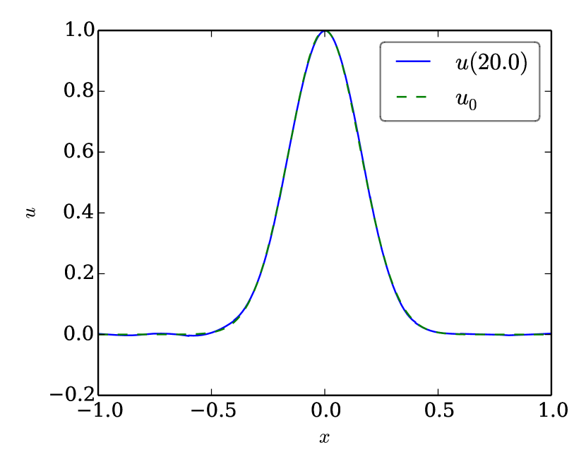
(b) $c=c_{0}$.

(c) $c=c_{SD}$.

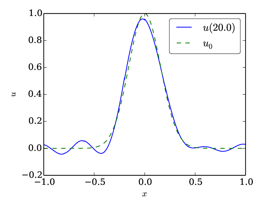
(d) $c=c_{Hu}$.

Figure 1: The numerical solution of constant velocity linear advection using SBP CPR methods with $10$ elements, a Lobatto-Legendre basis of order $p=3$ and a central numerical flux. Different values of $c$ are used for the correction matrix $\underline{\underline{C}}\,$. The initial Gaussian profile $u_{0}$ is shown in green, the numerical solution is plotted in blue.

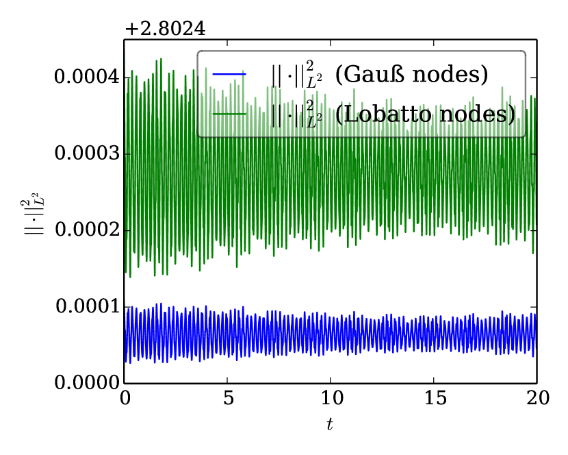
(a) $c=c_{-}/2$.

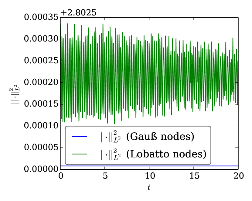
(b) $c=c_{0}$.

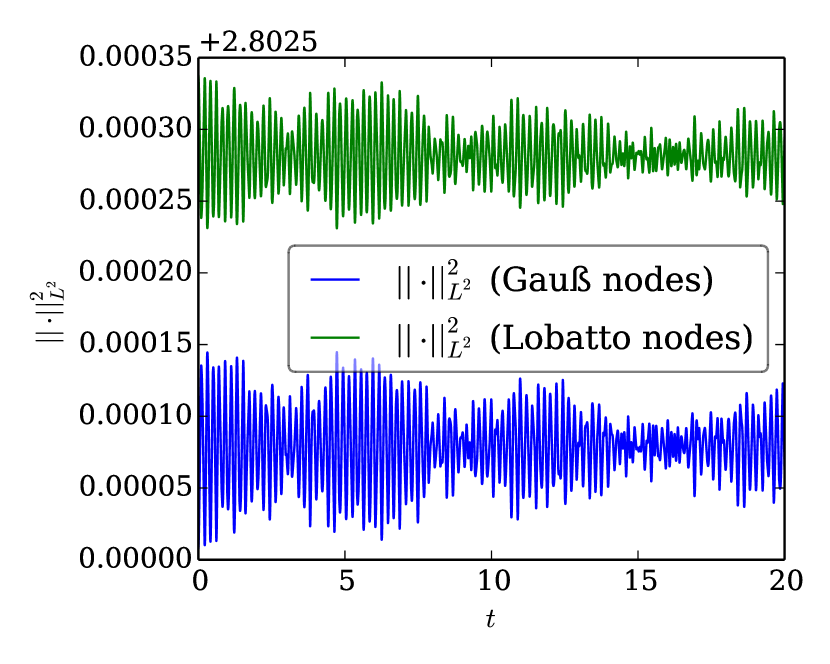
(c) $c=c_{SD}$.

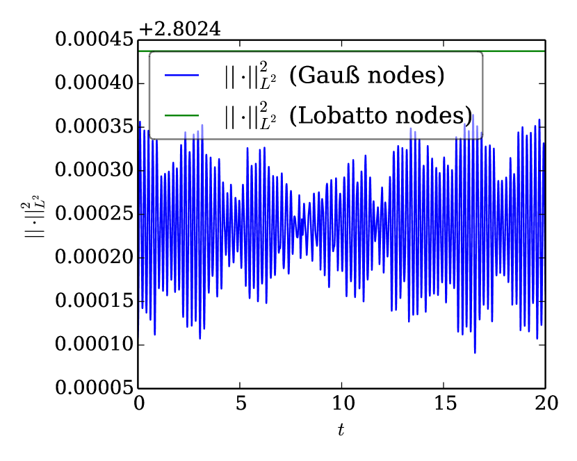
(d) $c=c_{Hu}$.

Figure 2: Energy of numerical solution of constant velocity linear advection using SBP CPR methods with $10$ elements, a Lobatto-Legendre basis of order $p=3$ and a central numerical flux. Different values of $c$ are used for the correction matrix $\underline{\underline{C}}\,$. The discrete energy $\mathinner{\!\left\lVert\underline{u}\right\rVert}^{2}$ is computed using Gauß-Legendre (blue) and Lobatto-Legendre (green) quadrature with $p+1=4$ nodes in the full time interval $[0,20]$.

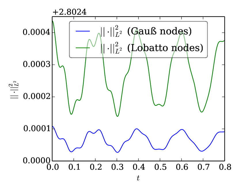
(a) $c=c_{-}/2$.

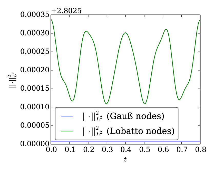
(b) $c=c_{0}$.

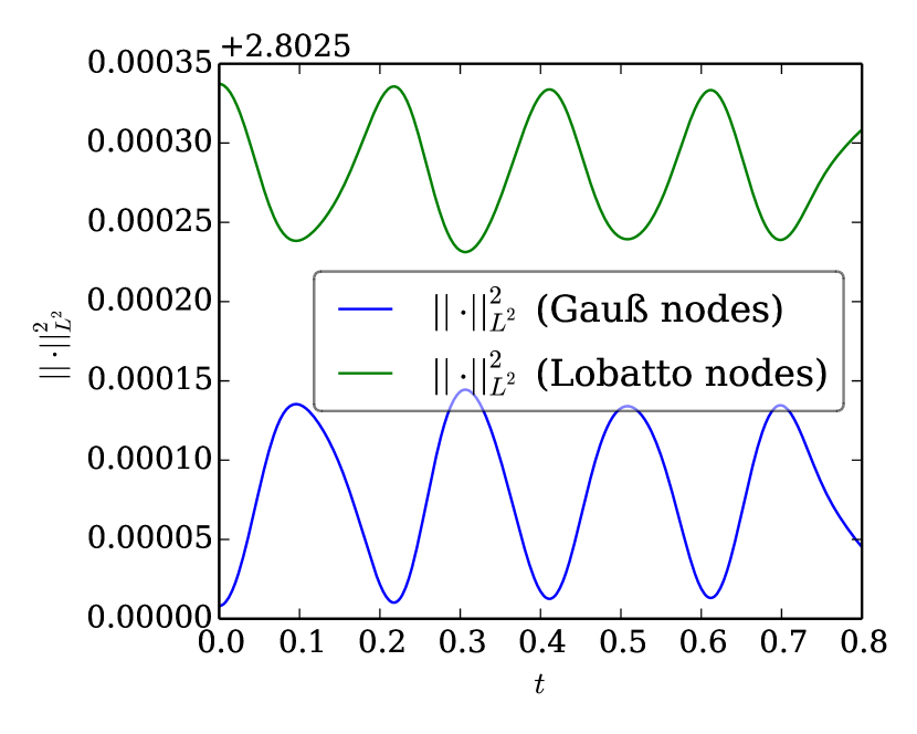
(c) $c=c_{SD}$.

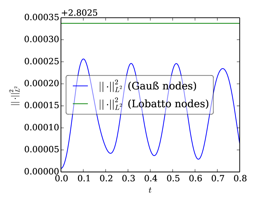
(d) $c=c_{Hu}$.

Figure 3: Energy of numerical solution of constant velocity linear advection using SBP CPR methods with $10$ elements, a Lobatto-Legendre basis of order $p=3$ and a central numerical flux. Different values of $c$ are used for the correction matrix $\underline{\underline{C}}\,$. The discrete energy $\mathinner{\!\left\lVert\underline{u}\right\rVert}^{2}$ is computed using Gauß-Legendre (blue) and Lobatto-Legendre (green) quadrature with $p+1=4$ nodes in the time interval $[0,0.8]$.

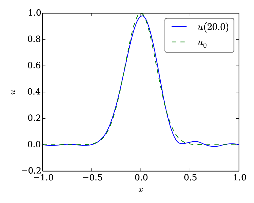
(a) $c=c_{-}/2$.

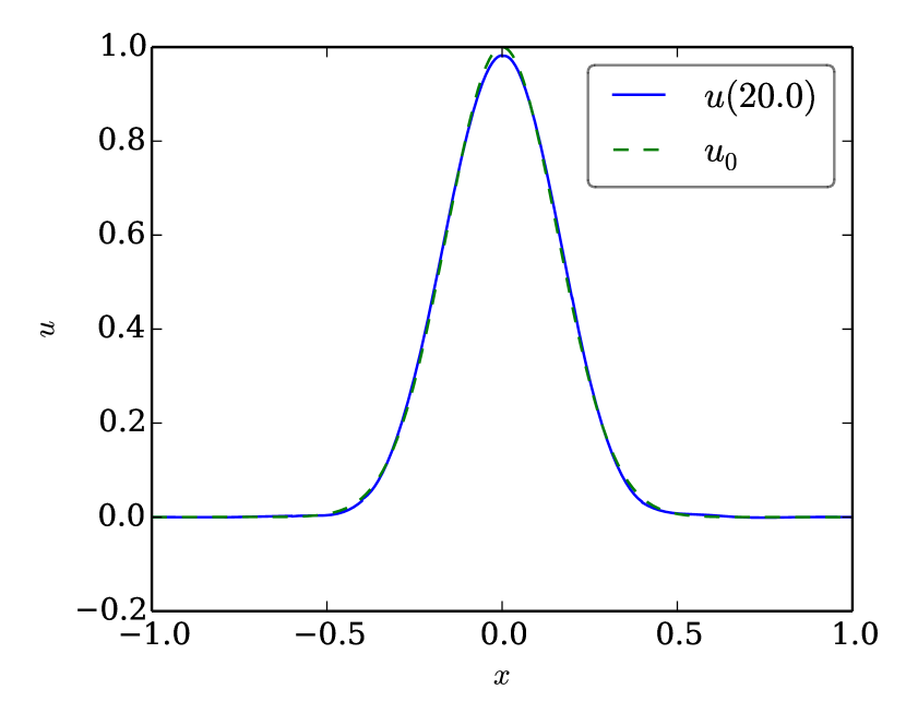
(b) $c=c_{0}$.

(c) $c=c_{SD}$.

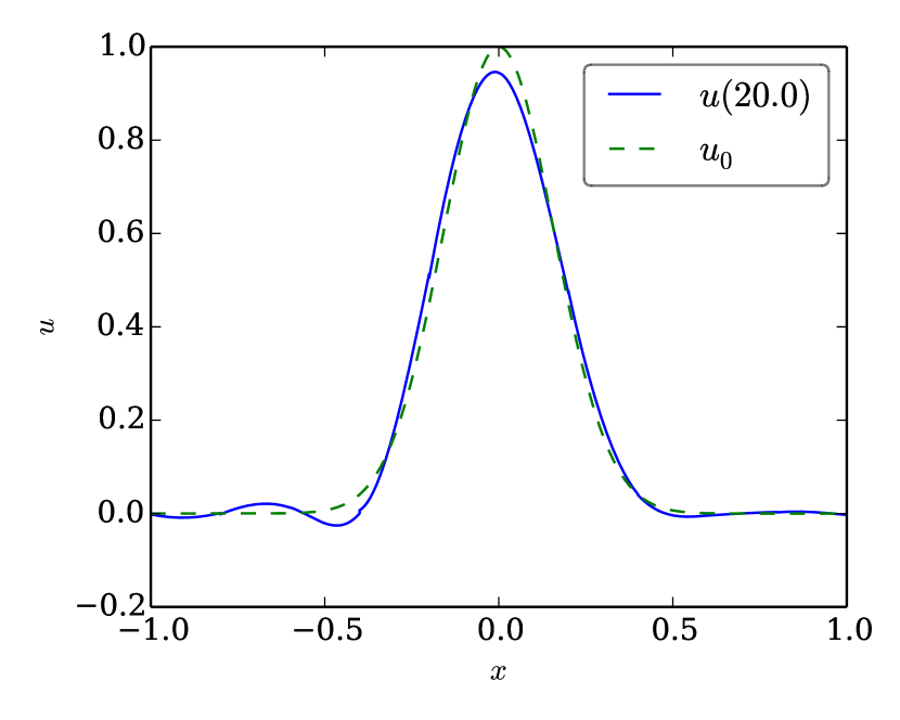
(d) $c=c_{Hu}$.

Figure 4: The numerical solution of constant velocity linear advection using SBP CPR methods with $10$ elements, a Lobatto-Legendre basis of order $p=3$ and a upwind numerical flux. Different values of $c$ are used for the correction matrix $\underline{\underline{C}}\,$. The initial Gaussian profile $u_{0}$ is shown in green, the numerical solution is plotted in blue.

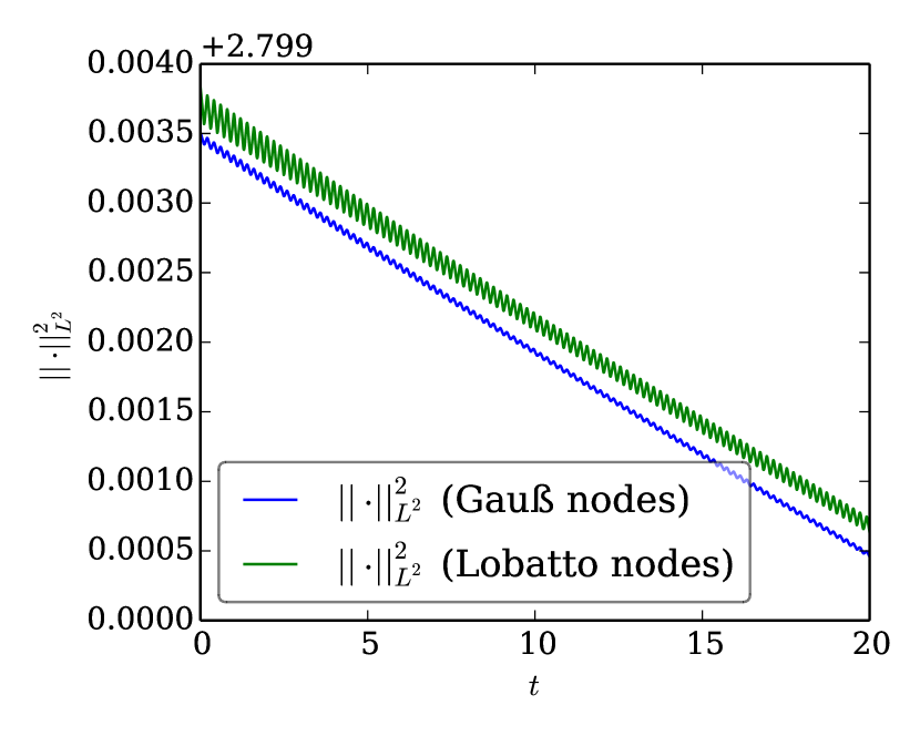
(a) $c=c_{-}/2$.

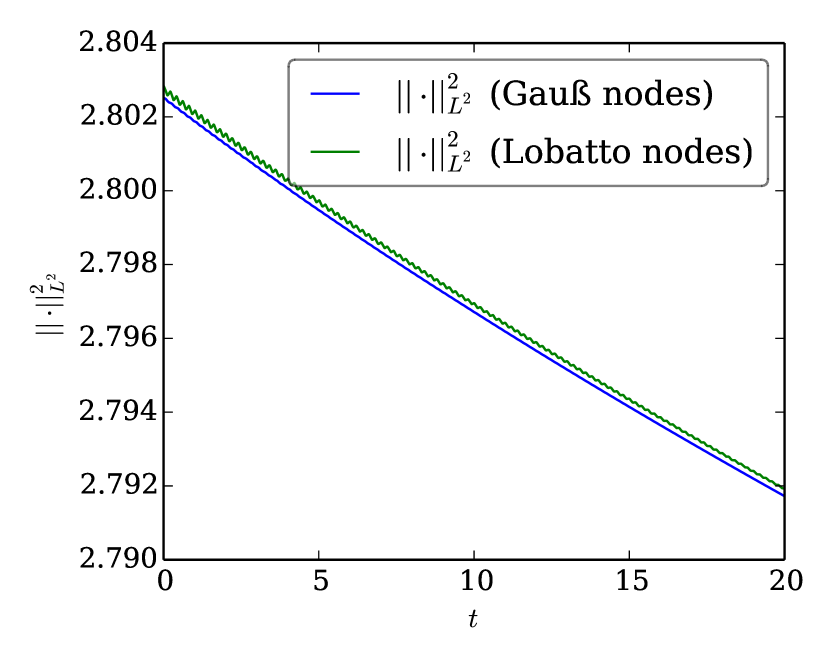
(b) $c=c_{0}$.

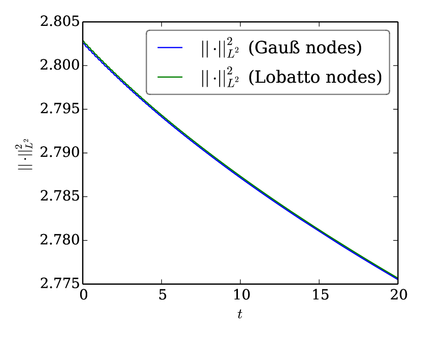
(c) $c=c_{SD}$.

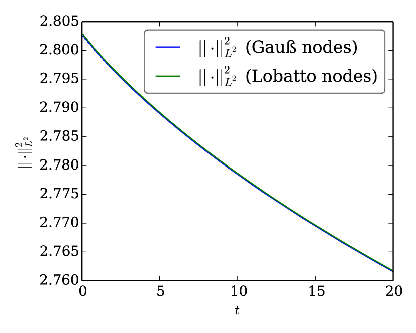
(d) $c=c_{Hu}$.

Figure 5: Energy of numerical solution of constant velocity linear advection using SBP CPR methods with $10$ elements, a Lobatto-Legendre basis of order $p=3$ and a upwind numerical flux. Different values of $c$ are used for the correction matrix $\underline{\underline{C}}\,$. The discrete energy $\mathinner{\!\left\lVert\underline{u}\right\rVert}^{2}$ is computed using Gauß-Legendre (blue) and Lobatto-Legendre (green) quadrature with $p+1=4$ nodes in the full time interval $[0,20]$.

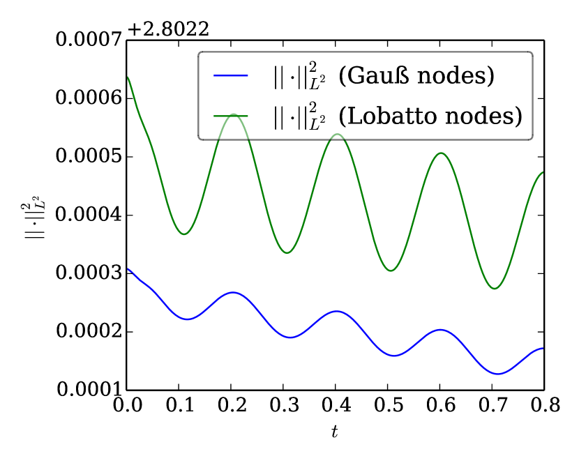
(a) $c=c_{-}/2$.

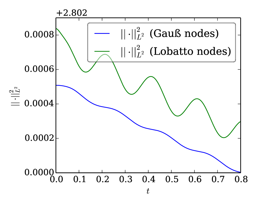
(b) $c=c_{0}$.

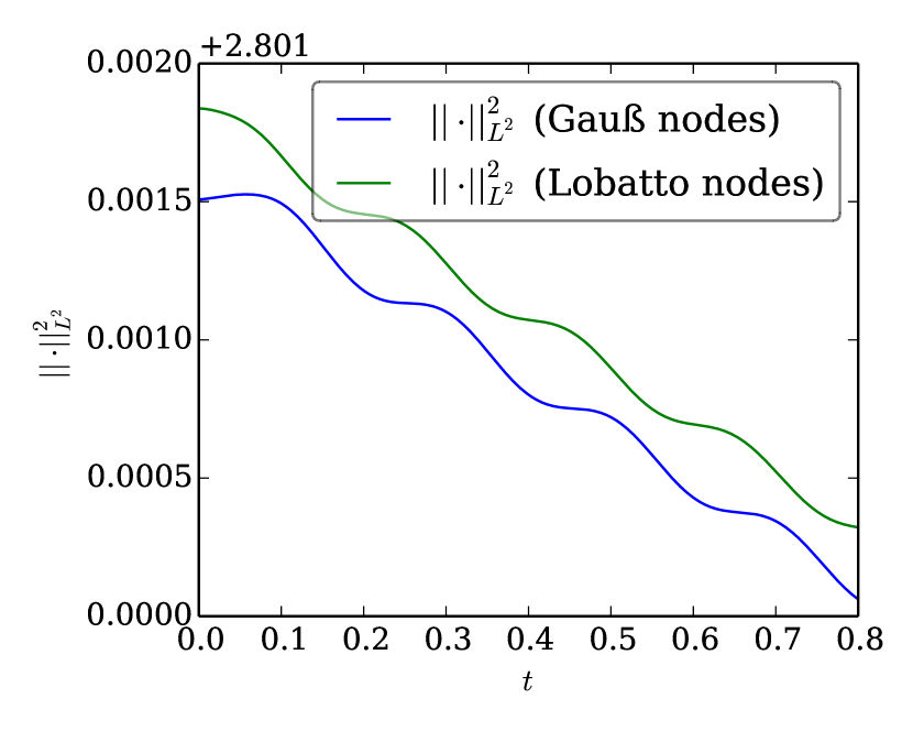
(c) $c=c_{SD}$.

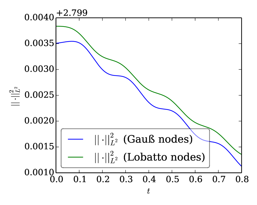
(d) $c=c_{Hu}$.

Figure 6: Energy of numerical solution of constant velocity linear advection using SBP CPR methods with $10$ elements, a Lobatto-Legendre basis of order $p=3$ and a upwind numerical flux. Different values of $c$ are used for the correction matrix $\underline{\underline{C}}\,$. The discrete energy $\mathinner{\!\left\lVert\underline{u}\right\rVert}^{2}$ is computed using Gauß-Legendre (blue) and Lobatto-Legendre (green) quadrature with $p+1=4$ nodes in the time interval $[0,0.8]$.

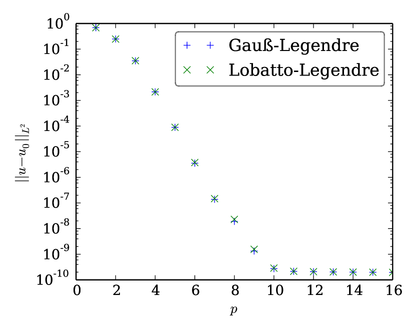
(a) $c=c_{-}/2$

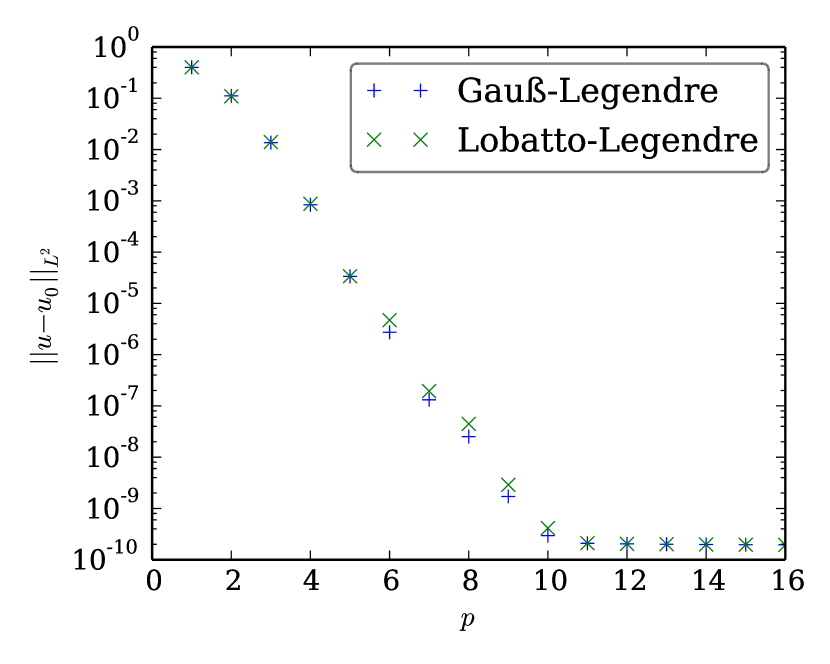
(b) $c=c_{0}$

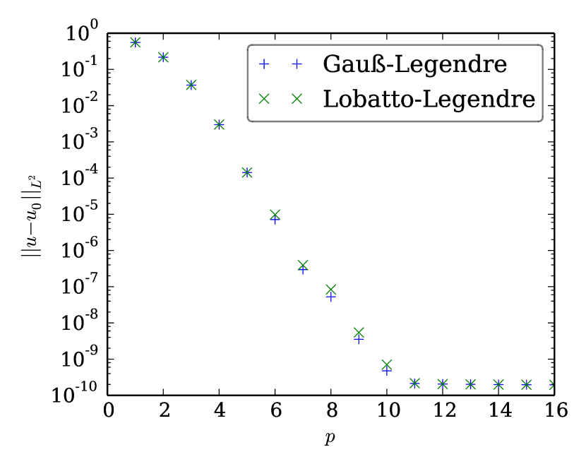
(c) $c=c_{SD}$

(d) $c=c_{Hu}$

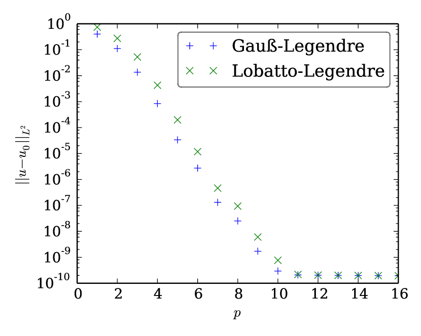
(e) $\kappa=0$

Figure 7: $L^{2}$ errors of $u(20)$ for constant velocity linear advection using SBP CPR methods with $N=10$ elements, a Gauß-Legendre and Lobatto-Legendre bases of varying order $p$ and an upwind numerical flux. Different values of $c$ are used for the correction matrix $\underline{\underline{C}}\,$.

Table 1: $L^{2}$ errors of $u(20)$ for constant velocity linear advection using SBP CPR methods with $N=10$ elements, Gauß-Legendre and Lobatto-Legendre bases of varying order $p$ and an upwind numerical flux. Different values of $c$ are used for the correction matrix $\underline{\underline{C}}\,$. Numerical values corresponding to Figure 7.

	$\mathinner{\!\left\lVert u-u_{0}\right\rVert}_{L^{2}}$
	$c=c_{-}/2$		$c=c_{0}$		$c=c_{SD}$		$c=c_{Hu}$
$p$	Gauß	Lobatto	Gauß	Lobatto	Gauß	Lobatto	Gauß	Lobatto
$1$	$6.88\text{\times}{10}^{-01}$	$6.86\text{\times}{10}^{-01}$	$4.00\text{\times}{10}^{-01}$	$4.03\text{\times}{10}^{-01}$	$5.55\text{\times}{10}^{-01}$	$5.59\text{\times}{10}^{-01}$	$7.40\text{\times}{10}^{-01}$	$7.41\text{\times}{10}^{-01}$
$2$	$2.49\text{\times}{10}^{-01}$	$2.47\text{\times}{10}^{-01}$	$1.12\text{\times}{10}^{-01}$	$1.09\text{\times}{10}^{-01}$	$2.17\text{\times}{10}^{-01}$	$2.16\text{\times}{10}^{-01}$	$2.75\text{\times}{10}^{-01}$	$2.74\text{\times}{10}^{-01}$
$3$	$3.51\text{\times}{10}^{-02}$	$3.55\text{\times}{10}^{-02}$	$1.36\text{\times}{10}^{-02}$	$1.40\text{\times}{10}^{-02}$	$3.70\text{\times}{10}^{-02}$	$3.74\text{\times}{10}^{-02}$	$5.22\text{\times}{10}^{-02}$	$5.27\text{\times}{10}^{-02}$
$4$	$2.16\text{\times}{10}^{-03}$	$2.15\text{\times}{10}^{-03}$	$8.38\text{\times}{10}^{-04}$	$8.75\text{\times}{10}^{-04}$	$2.98\text{\times}{10}^{-03}$	$3.01\text{\times}{10}^{-03}$	$4.26\text{\times}{10}^{-03}$	$4.28\text{\times}{10}^{-03}$
$5$	$8.92\text{\times}{10}^{-05}$	$8.93\text{\times}{10}^{-05}$	$3.36\text{\times}{10}^{-05}$	$3.38\text{\times}{10}^{-05}$	$1.42\text{\times}{10}^{-04}$	$1.42\text{\times}{10}^{-04}$	$1.98\text{\times}{10}^{-04}$	$1.98\text{\times}{10}^{-04}$
$6$	$3.56\text{\times}{10}^{-06}$	$3.77\text{\times}{10}^{-06}$	$2.73\text{\times}{10}^{-06}$	$4.71\text{\times}{10}^{-06}$	$7.16\text{\times}{10}^{-06}$	$9.81\text{\times}{10}^{-06}$	$9.04\text{\times}{10}^{-06}$	$1.18\text{\times}{10}^{-05}$
$7$	$1.39\text{\times}{10}^{-07}$	$1.48\text{\times}{10}^{-07}$	$1.32\text{\times}{10}^{-07}$	$1.95\text{\times}{10}^{-07}$	$2.97\text{\times}{10}^{-07}$	$3.93\text{\times}{10}^{-07}$	$3.61\text{\times}{10}^{-07}$	$4.64\text{\times}{10}^{-07}$
$8$	$1.90\text{\times}{10}^{-08}$	$2.28\text{\times}{10}^{-08}$	$2.52\text{\times}{10}^{-08}$	$4.46\text{\times}{10}^{-08}$	$5.25\text{\times}{10}^{-08}$	$8.38\text{\times}{10}^{-08}$	$6.03\text{\times}{10}^{-08}$	$9.40\text{\times}{10}^{-08}$
$9$	$1.33\text{\times}{10}^{-09}$	$1.55\text{\times}{10}^{-09}$	$1.71\text{\times}{10}^{-09}$	$2.89\text{\times}{10}^{-09}$	$3.53\text{\times}{10}^{-09}$	$5.45\text{\times}{10}^{-09}$	$4.00\text{\times}{10}^{-09}$	$6.05\text{\times}{10}^{-09}$
$10$	$2.73\text{\times}{10}^{-10}$	$2.88\text{\times}{10}^{-10}$	$2.95\text{\times}{10}^{-10}$	$4.13\text{\times}{10}^{-10}$	$4.77\text{\times}{10}^{-10}$	$7.05\text{\times}{10}^{-10}$	$5.23\text{\times}{10}^{-10}$	$7.68\text{\times}{10}^{-10}$
$11$	$2.15\text{\times}{10}^{-10}$	$2.15\text{\times}{10}^{-10}$	$2.09\text{\times}{10}^{-10}$	$2.10\text{\times}{10}^{-10}$	$2.13\text{\times}{10}^{-10}$	$2.17\text{\times}{10}^{-10}$	$2.14\text{\times}{10}^{-10}$	$2.18\text{\times}{10}^{-10}$
$12$	$2.09\text{\times}{10}^{-10}$	$2.09\text{\times}{10}^{-10}$	$2.04\text{\times}{10}^{-10}$	$2.04\text{\times}{10}^{-10}$	$2.05\text{\times}{10}^{-10}$	$2.05\text{\times}{10}^{-10}$	$2.05\text{\times}{10}^{-10}$	$2.06\text{\times}{10}^{-10}$
$13$	$2.04\text{\times}{10}^{-10}$	$2.04\text{\times}{10}^{-10}$	$2.01\text{\times}{10}^{-10}$	$2.01\text{\times}{10}^{-10}$	$2.01\text{\times}{10}^{-10}$	$2.01\text{\times}{10}^{-10}$	$2.02\text{\times}{10}^{-10}$	$2.02\text{\times}{10}^{-10}$
$14$	$2.01\text{\times}{10}^{-10}$	$2.01\text{\times}{10}^{-10}$	$1.98\text{\times}{10}^{-10}$	$1.98\text{\times}{10}^{-10}$	$1.99\text{\times}{10}^{-10}$	$1.99\text{\times}{10}^{-10}$	$1.99\text{\times}{10}^{-10}$	$1.99\text{\times}{10}^{-10}$
$15$	$1.98\text{\times}{10}^{-10}$	$1.98\text{\times}{10}^{-10}$	$1.96\text{\times}{10}^{-10}$	$1.96\text{\times}{10}^{-10}$	$1.97\text{\times}{10}^{-10}$	$1.97\text{\times}{10}^{-10}$	$1.97\text{\times}{10}^{-10}$	$1.97\text{\times}{10}^{-10}$
$16$	$1.96\text{\times}{10}^{-10}$	$1.96\text{\times}{10}^{-10}$	$1.95\text{\times}{10}^{-10}$	$1.95\text{\times}{10}^{-10}$	$1.95\text{\times}{10}^{-10}$	$1.95\text{\times}{10}^{-10}$	$1.95\text{\times}{10}^{-10}$	$1.95\text{\times}{10}^{-10}$

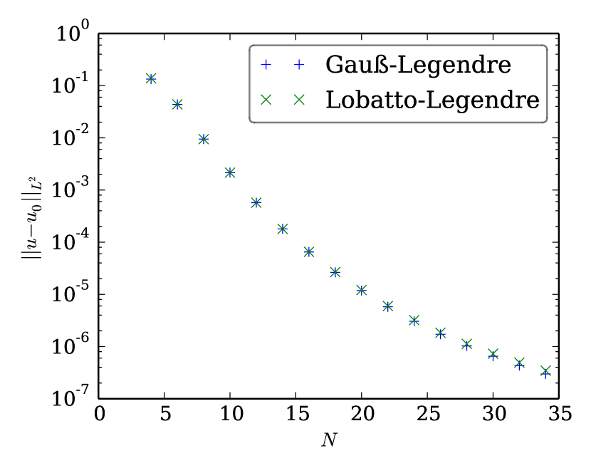
(a) $c=c_{-}/2$

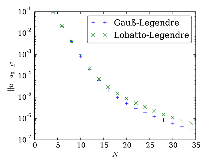
(b) $c=c_{0}$

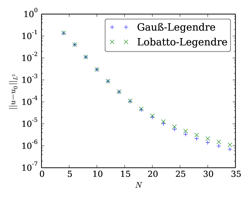
(c) $c=c_{SD}$

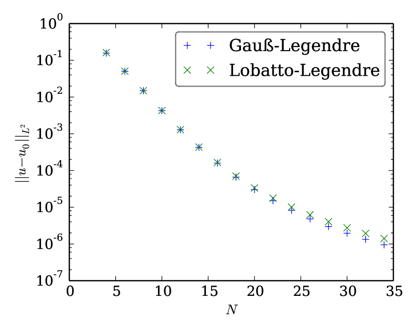
(d) $c=c_{Hu}$

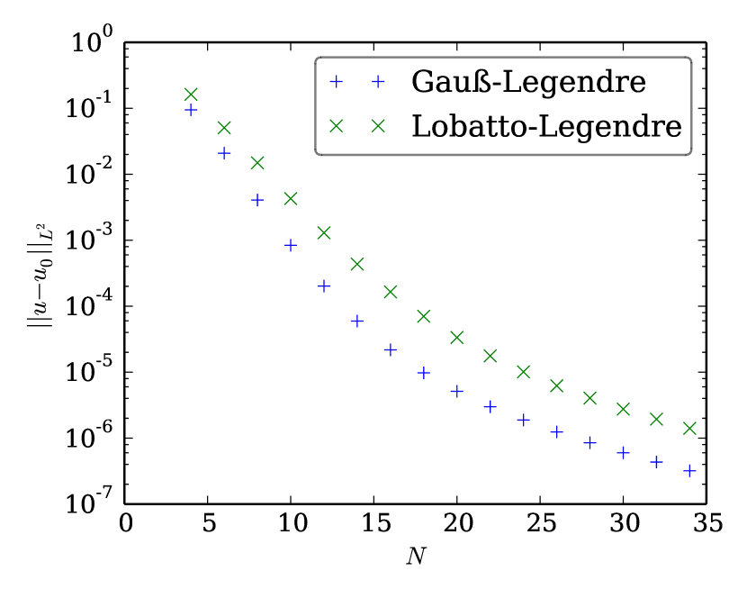
(e) $\kappa=0$

Figure 8: $L^{2}$ errors of $u(20)$ for constant velocity linear advection using SBP CPR methods with varying number of elements $N$, Gauß-Legendre and Lobatto-Legendre bases of order $p=4$ and an upwind numerical flux. Different values of $c$ are used for the correction matrix $\underline{\underline{C}}\,$.

Table 2: $L^{2}$ errors of $u(20)$ for constant velocity linear advection using SBP CPR methods with varying number of elements $N$, Gauß-Legendre and Lobatto-Legendre bases of order $p=4$ and an upwind numerical flux. Different values of $c$ are used for the correction matrix $\underline{\underline{C}}\,$. Numerical values corresponding to Figure 8.

	$\mathinner{\!\left\lVert u-u_{0}\right\rVert}_{L^{2}}$
	$c=c_{-}/2$		$c=c_{0}$		$c=c_{SD}$		$c=c_{Hu}$
$N$	Gauß	Lobatto	Gauß	Lobatto	Gauß	Lobatto	Gauß	Lobatto
$4$	$1.34\text{\times}{10}^{-01}$	$1.39\text{\times}{10}^{-01}$	$9.48\text{\times}{10}^{-02}$	$9.99\text{\times}{10}^{-02}$	$1.35\text{\times}{10}^{-01}$	$1.40\text{\times}{10}^{-01}$	$1.57\text{\times}{10}^{-01}$	$1.62\text{\times}{10}^{-01}$
$6$	$4.37\text{\times}{10}^{-02}$	$4.38\text{\times}{10}^{-02}$	$2.09\text{\times}{10}^{-02}$	$2.12\text{\times}{10}^{-02}$	$4.05\text{\times}{10}^{-02}$	$4.08\text{\times}{10}^{-02}$	$5.04\text{\times}{10}^{-02}$	$5.07\text{\times}{10}^{-02}$
$8$	$9.46\text{\times}{10}^{-03}$	$9.44\text{\times}{10}^{-03}$	$4.06\text{\times}{10}^{-03}$	$4.13\text{\times}{10}^{-03}$	$1.11\text{\times}{10}^{-02}$	$1.11\text{\times}{10}^{-02}$	$1.49\text{\times}{10}^{-02}$	$1.49\text{\times}{10}^{-02}$
$10$	$2.16\text{\times}{10}^{-03}$	$2.15\text{\times}{10}^{-03}$	$8.38\text{\times}{10}^{-04}$	$8.75\text{\times}{10}^{-04}$	$2.98\text{\times}{10}^{-03}$	$3.01\text{\times}{10}^{-03}$	$4.26\text{\times}{10}^{-03}$	$4.28\text{\times}{10}^{-03}$
$12$	$5.73\text{\times}{10}^{-04}$	$5.71\text{\times}{10}^{-04}$	$2.02\text{\times}{10}^{-04}$	$2.23\text{\times}{10}^{-04}$	$8.65\text{\times}{10}^{-04}$	$8.80\text{\times}{10}^{-04}$	$1.28\text{\times}{10}^{-03}$	$1.30\text{\times}{10}^{-03}$
$14$	$1.80\text{\times}{10}^{-04}$	$1.80\text{\times}{10}^{-04}$	$5.95\text{\times}{10}^{-05}$	$7.20\text{\times}{10}^{-05}$	$2.83\text{\times}{10}^{-04}$	$2.91\text{\times}{10}^{-04}$	$4.27\text{\times}{10}^{-04}$	$4.35\text{\times}{10}^{-04}$
$16$	$6.50\text{\times}{10}^{-05}$	$6.54\text{\times}{10}^{-05}$	$2.18\text{\times}{10}^{-05}$	$3.01\text{\times}{10}^{-05}$	$1.05\text{\times}{10}^{-04}$	$1.11\text{\times}{10}^{-04}$	$1.59\text{\times}{10}^{-04}$	$1.65\text{\times}{10}^{-04}$
$18$	$2.64\text{\times}{10}^{-05}$	$2.68\text{\times}{10}^{-05}$	$9.75\text{\times}{10}^{-06}$	$1.52\text{\times}{10}^{-05}$	$4.36\text{\times}{10}^{-05}$	$4.80\text{\times}{10}^{-05}$	$6.60\text{\times}{10}^{-05}$	$7.04\text{\times}{10}^{-05}$
$20$	$1.19\text{\times}{10}^{-05}$	$1.21\text{\times}{10}^{-05}$	$5.12\text{\times}{10}^{-06}$	$8.64\text{\times}{10}^{-06}$	$2.01\text{\times}{10}^{-05}$	$2.34\text{\times}{10}^{-05}$	$3.03\text{\times}{10}^{-05}$	$3.35\text{\times}{10}^{-05}$
$22$	$5.79\text{\times}{10}^{-06}$	$5.99\text{\times}{10}^{-06}$	$3.00\text{\times}{10}^{-06}$	$5.29\text{\times}{10}^{-06}$	$1.02\text{\times}{10}^{-05}$	$1.27\text{\times}{10}^{-05}$	$1.52\text{\times}{10}^{-05}$	$1.77\text{\times}{10}^{-05}$
$24$	$3.05\text{\times}{10}^{-06}$	$3.20\text{\times}{10}^{-06}$	$1.88\text{\times}{10}^{-06}$	$3.41\text{\times}{10}^{-06}$	$5.65\text{\times}{10}^{-06}$	$7.45\text{\times}{10}^{-06}$	$8.24\text{\times}{10}^{-06}$	$1.01\text{\times}{10}^{-05}$
$26$	$1.72\text{\times}{10}^{-06}$	$1.84\text{\times}{10}^{-06}$	$1.24\text{\times}{10}^{-06}$	$2.28\text{\times}{10}^{-06}$	$3.36\text{\times}{10}^{-06}$	$4.68\text{\times}{10}^{-06}$	$4.81\text{\times}{10}^{-06}$	$6.22\text{\times}{10}^{-06}$
$28$	$1.03\text{\times}{10}^{-06}$	$1.13\text{\times}{10}^{-06}$	$8.51\text{\times}{10}^{-07}$	$1.57\text{\times}{10}^{-06}$	$2.12\text{\times}{10}^{-06}$	$3.10\text{\times}{10}^{-06}$	$2.99\text{\times}{10}^{-06}$	$4.05\text{\times}{10}^{-06}$
$30$	$6.51\text{\times}{10}^{-07}$	$7.29\text{\times}{10}^{-07}$	$6.00\text{\times}{10}^{-07}$	$1.11\text{\times}{10}^{-06}$	$1.41\text{\times}{10}^{-06}$	$2.13\text{\times}{10}^{-06}$	$1.96\text{\times}{10}^{-06}$	$2.75\text{\times}{10}^{-06}$
$32$	$4.32\text{\times}{10}^{-07}$	$4.93\text{\times}{10}^{-07}$	$4.34\text{\times}{10}^{-07}$	$8.08\text{\times}{10}^{-07}$	$9.76\text{\times}{10}^{-07}$	$1.52\text{\times}{10}^{-06}$	$1.34\text{\times}{10}^{-06}$	$1.94\text{\times}{10}^{-06}$
$34$	$2.98\text{\times}{10}^{-07}$	$3.46\text{\times}{10}^{-07}$	$3.20\text{\times}{10}^{-07}$	$5.97\text{\times}{10}^{-07}$	$6.98\text{\times}{10}^{-07}$	$1.11\text{\times}{10}^{-06}$	$9.49\text{\times}{10}^{-07}$	$1.41\text{\times}{10}^{-06}$

3.9 Influence of time discretisation

Leaving the mathematical paradise of the previous sections and entering the real world of numerical methods, time discretisation plays an important role. For simplicity, an explicit Euler method for an SBP CPR semidiscretisation of the linear advection equation (14) is considered. Thus, one step of size $\Delta t$ from $\underline{u}$ to $\underline{u}^{+}$ (in the standard element) can be written as

$$\underline{u}^{+}=\underline{u}+\Delta t\,\partial_{t}\underline{u}.$$ (63)

Thus, the discrete norm after one time step is

$${\underline{u}^{+}}^{T}\underline{\underline{M}}\,\underline{u}^{+} =\left(\underline{u}+\Delta t\,\partial_{t}\underline{u}\right)^{T}\underline{\underline{M}}\,\left(\underline{u}+\Delta t\,\partial_{t}\underline{u}\right)$$ (64)

$$=\underline{u}^{T}\underline{\underline{M}}\,\underline{u}+2\Delta t\,\underline{u}^{T}\underline{\underline{M}}\,\partial_{t}\underline{u}+\Delta t^{2}\,\partial_{t}\underline{u}^{T}\underline{\underline{M}}\,\partial_{t}\underline{u}.$$

The computations leading to Lemma 2 result in an estimate of the second term $\underline{u}^{T}\underline{\underline{M}}\,\partial_{t}\underline{u}\leq 0$. Since $\underline{\underline{M}}\,$ is positive definite, the third term is non-negative (for $\Delta t>0$). Thus, time discretisation introduces a growth of the discrete norm not considered in the previous calculations, possibly leading to stability issues. In order to get a decay of the discrete norm, the difference

$${\underline{u}^{+}}^{T}\underline{\underline{M}}\,\underline{u}^{+}-\underline{u}^{T}\underline{\underline{M}}\,\underline{u}=2\Delta t\left(\underline{u}+\frac{\Delta t}{2}\partial_{t}\underline{u}\right)^{T}\underline{\underline{M}}\,\partial_{t}\underline{u}$$ (65)

must be estimated. Inserting the SBP CPR semidiscretisation for the linear advection equation with constant velocity yields

$$\left(\underline{u}+\frac{\Delta t}{2}\partial_{t}\underline{u}\right)^{T}\underline{\underline{M}}\,\partial_{t}\underline{u}$$ (66)

$$=\left(\underline{u}-\frac{\Delta t}{2}\underline{\underline{D}}\,\underline{u}-\frac{\Delta t}{2}\underline{\underline{C}}\,(\underline{f}^{num}-\underline{\underline{R}}\,\underline{u})\right)^{T}\underline{\underline{M}}\,\left(-\underline{\underline{D}}\,\underline{u}-\underline{\underline{C}}\,(\underline{f}^{num}-\underline{\underline{R}}\,\underline{u})\right)$$

$$=-\underline{u}^{T}\underline{\underline{M}}\,\underline{\underline{D}}\,\underline{u}-\underline{u}^{T}\underline{\underline{M}}\,\underline{\underline{C}}\,(\underline{f}^{num}-\underline{\underline{R}}\,\underline{u})$$

$$\quad+\frac{\Delta t}{2}\left[\underline{u}^{T}\underline{\underline{D}}\,^{T}\underline{\underline{M}}\,\underline{\underline{D}}\,\underline{u}+(\underline{f}^{num}-\underline{\underline{R}}\,\underline{u})^{T}\underline{\underline{C}}\,^{T}\underline{\underline{M}}\,\underline{\underline{C}}\,(\underline{f}^{num}-\underline{\underline{R}}\,\underline{u})\right]$$

$$\quad\left.+2\underline{u}^{T}\underline{\underline{D}}\,^{T}\underline{\underline{M}}\,\underline{\underline{C}}\,(\underline{f}^{num}-\underline{\underline{R}}\,\underline{u})\right].$$

Inserting $\underline{\underline{C}}\,=\underline{\underline{M}}\,^{-1}\underline{\underline{R}}\,^{T}\underline{\underline{B}}\,$, the right hand side becomes

$$-\underline{u}^{T}\underline{\underline{M}}\,\underline{\underline{D}}\,\underline{u}-\underline{u}^{T}\underline{\underline{R}}\,^{T}\underline{\underline{B}}\,(\underline{f}^{num}-\underline{\underline{R}}\,\underline{u})$$ (67)

$$+\frac{\Delta t}{2}\left[\underline{u}^{T}\underline{\underline{D}}\,^{T}\underline{\underline{M}}\,\underline{\underline{D}}\,\underline{u}+(\underline{f}^{num}-\underline{\underline{R}}\,\underline{u})^{T}\underline{\underline{B}}\,^{T}\underline{\underline{R}}\,\underline{\underline{M}}\,^{-1}\underline{\underline{R}}\,^{T}\underline{\underline{B}}\,(\underline{f}^{num}-\underline{\underline{R}}\,\underline{u})\right.$$

$$\left.+2\underline{u}^{T}\underline{\underline{D}}\,^{T}\underline{\underline{R}}\,^{T}\underline{\underline{B}}\,(\underline{f}^{num}-\underline{\underline{R}}\,\underline{u})\right].$$

Using the SBP property $\underline{\underline{M}}\,\underline{\underline{D}}\,+\underline{\underline{D}}\,^{T}\underline{\underline{M}}\,=\underline{\underline{R}}\,^{T}\underline{\underline{B}}\,\underline{\underline{R}}\,$ results in

$$\underline{u}^{T}\underline{\underline{D}}\,^{T}\underline{\underline{M}}\,\underline{u}-\underline{u}^{T}\underline{\underline{R}}\,^{T}\underline{\underline{B}}\,\underline{\underline{R}}\,\underline{u}-\underline{u}^{T}\underline{\underline{R}}\,^{T}\underline{\underline{B}}\,(\underline{f}^{num}-\underline{\underline{R}}\,\underline{u})$$ (68)

$$+\frac{\Delta t}{2}\left[\underline{u}^{T}\underline{\underline{D}}\,^{T}\underline{\underline{M}}\,\underline{\underline{D}}\,\underline{u}+(\underline{f}^{num}-\underline{\underline{R}}\,\underline{u})^{T}\underline{\underline{B}}\,^{T}\underline{\underline{R}}\,\underline{\underline{M}}\,^{-1}\underline{\underline{R}}\,^{T}\underline{\underline{B}}\,(\underline{f}^{num}-\underline{\underline{R}}\,\underline{u})\right.$$

$$+\left.+2\underline{u}^{T}\underline{\underline{D}}\,^{T}\underline{\underline{R}}\,^{T}\underline{\underline{B}}\,(\underline{f}^{num}-\underline{\underline{R}}\,\underline{u})\right].$$

Thus, adding these expressions, the left hand side $LHS$ can be expressed as

$$2\,LHS=\underline{u}^{T}\underline{\underline{R}}\,^{T}\underline{\underline{B}}\,\underline{\underline{R}}\,\underline{u}-2\underline{u}^{T}\underline{\underline{R}}\,^{T}\underline{\underline{B}}\,\underline{f}^{num}$$ (69)

$$\quad+\Delta t\left[\underline{u}^{T}\underline{\underline{D}}\,^{T}\underline{\underline{M}}\,\underline{\underline{D}}\,\underline{u}+(\underline{f}^{num}-\underline{\underline{R}}\,\underline{u})^{T}\underline{\underline{B}}\,^{T}\underline{\underline{R}}\,\underline{\underline{M}}\,^{-1}\underline{\underline{R}}\,^{T}\underline{\underline{B}}\,(\underline{f}^{num}-\underline{\underline{R}}\,\underline{u})\right.$$

$$\quad\left.+2\underline{u}^{T}\underline{\underline{D}}\,^{T}\underline{\underline{R}}\,^{T}\underline{\underline{B}}\,(\underline{f}^{num}-\underline{\underline{R}}\,\underline{u})\right].$$

If all summands on the right hand side would involve only boundary terms, an estimate similar to those in previous sections would be possible. Unfortunately, the volume term $\underline{u}^{T}\underline{\underline{D}}\,^{T}\underline{\underline{M}}\,\underline{\underline{D}}\,\underline{u}$ does not seem to allow such an estimate. Therefore, an estimate leading to fully discrete stability for an explicit Euler method does not seem to be possible in this straightforward calculation. Thus, for practical calculations, a time discretisation with high accuracy should be chosen in order to avoid stability issues. Note that the non-positive stability result for the explicit Euler methods extends directly to standard SSP time discretisations consisting of convex combinations of Euler steps.

4 CPR methods using SBP operators: Burgers’ equation

Stability properties for linear and nonlinear problems can be very different. Thus, although stability for linear advection with constant velocity can be proven for several SBP CPR schemes (see Theorem 5), these results do not imply nonlinear stability. For simplicity, the (inviscid) Burgers’ equation

$$\partial_{t}u+\partial_{x}\frac{u^{2}}{2}=0$$ (70)

in one space dimension with periodic boundary conditions and appropriate initial condition is considered.

4.1 Nonlinear stability

A straightforward application of an SBP CPR method can be written as

$$\partial_{t}\underline{u}+\frac{1}{2}\underline{\underline{D}}\,\underline{u^{2}}+\underline{\underline{C}}\,(\underline{f}^{num}-\frac{1}{2}\underline{\underline{R}}\,\underline{u^{2}})=0$$ (71)

for the standard element. Estimating the discrete norm similar to the previous sections results in

$$\underline{u}^{T}\underline{\underline{M}}\,\partial_{t}\underline{u}=-\frac{1}{2}\underline{u}^{T}\underline{\underline{M}}\,\underline{\underline{D}}\,\underline{u^{2}}-\underline{u}^{T}\underline{\underline{M}}\,\underline{\underline{C}}\,(\underline{f}^{num}-\frac{1}{2}\underline{\underline{R}}\,\underline{u^{2}}).$$ (72)

Applying the SBP property and $\underline{\underline{M}}\,\underline{\underline{C}}\,=\underline{\underline{R}}\,^{T}\underline{\underline{B}}\,$ yields

$$\frac{1}{2}\dfrac{\operatorname{d\!}{}}{\operatorname{d\!}{t}}\mathinner{\!\left\lVert u\right\rVert}_{M}^{2}=\frac{1}{2}\underline{u}^{T}\underline{\underline{D}}\,^{T}\underline{\underline{M}}\,\underline{u^{2}}-\frac{1}{2}\underline{u}^{T}\underline{\underline{R}}\,^{T}\underline{\underline{B}}\,\underline{\underline{R}}\,\underline{u^{2}}-\underline{u}^{T}\underline{\underline{R}}\,^{T}\underline{\underline{B}}\,(\underline{f}^{num}-\frac{1}{2}\underline{\underline{R}}\,\underline{u^{2}}).$$ (73)

Unfortunately, the nonlinear flux does not allow a cancellation of boundary terms as in the linear case. A possibility to overcome this problem in the setting of DG spectral element methods was investigated by Gassner [8]. There, he uses Lobatto-Legendre interpolation polynomials as nodal basis and a skew-symmetric form of the conservation law

$$\partial_{t}u+\alpha\partial_{x}\frac{u^{2}}{2}+(1-\alpha)u\partial_{x}u=0,\quad 0\leq\alpha\leq 1.$$ (74)

Thus, the divergence of the flux is written as a convex combination of the two terms $\partial_{x}\frac{u^{2}}{2}$ and $u\partial_{x}u$ which are exactly equal if the product rule of differentiation is valid for $\partial_{x}$. The discrete derivative operator $\underline{\underline{D}}\,$ does not fulfil this product rule and therefore, the split operator form (74) can be regarded as the standard conservative form (70) with an additional correction term

$$\partial_{t}u+\partial_{x}\frac{u^{2}}{2}+(1-\alpha)\left(u\partial_{x}u-\partial_{x}\frac{u^{2}}{2}\right)=0.$$ (75)

Using the SBP CPR semidiscretisation for this equation results is

$$\partial_{t}\underline{u}=-\frac{1}{2}\underline{\underline{D}}\,\underline{u^{2}}-(1-\alpha)(\underline{\underline{u}}\,\underline{\underline{D}}\,\underline{u}-\frac{1}{2}\underline{\underline{D}}\,\underline{u^{2}})-\underline{\underline{C}}\,(\underline{f}^{num}-\frac{1}{2}\underline{\underline{R}}\,\underline{u^{2}})=0.$$ (76)

Here, $\underline{\underline{u}}\,=\operatorname{diag}(\underline{u})$ denotes the matrix representing multiplication with $u$. Now, multiplication with $\underline{u}^{T}\underline{\underline{M}}\,$ results in

$$\frac{1}{2}\dfrac{\operatorname{d\!}{}}{\operatorname{d\!}{t}}\mathinner{\!\left\lVert u\right\rVert}_{M}^{2}=-\frac{\alpha}{2}\underline{u}^{T}\underline{\underline{M}}\,\underline{\underline{D}}\,\underline{u^{2}}-(1-\alpha)\underline{u}^{T}\underline{\underline{M}}\,\underline{\underline{u}}\,\underline{\underline{D}}\,\underline{u}-\underline{u}^{T}\underline{\underline{M}}\,\underline{\underline{C}}\,(\underline{f}^{num}-\frac{1}{2}\underline{\underline{R}}\,\underline{u^{2}}).$$ (77)

Using $\underline{\underline{C}}\,=\underline{\underline{M}}\,^{-1}\underline{\underline{R}}\,^{T}\underline{\underline{B}}\,$ and $\underline{u^{2}}=\underline{\underline{u}}\,\underline{u}$, this can be written as

$$\frac{1}{2}\dfrac{\operatorname{d\!}{}}{\operatorname{d\!}{t}}\mathinner{\!\left\lVert u\right\rVert}_{M}^{2}= -\frac{\alpha}{2}\underline{u}^{T}\underline{\underline{M}}\,\underline{\underline{D}}\,\underline{\underline{u}}\,\underline{u}-(1-\alpha)\underline{u}^{T}\underline{\underline{M}}\,\underline{\underline{u}}\,\underline{\underline{D}}\,\underline{u}$$ (78)

$$-\underline{u}^{T}\underline{\underline{R}}\,^{T}\underline{\underline{B}}\,\underline{f}^{num}+\frac{1}{2}\underline{u}^{T}\underline{\underline{R}}\,^{T}\underline{\underline{B}}\,\underline{\underline{R}}\,\underline{\underline{u}}\,\underline{u}.$$

Since a nodal Lobatto-Legendre basis with lumped mass matrix is chosen, both $\underline{\underline{u}}\,$ and $\underline{\underline{M}}\,$ are diagonal and therefore commute

$$\frac{1}{2}\dfrac{\operatorname{d\!}{}}{\operatorname{d\!}{t}}\mathinner{\!\left\lVert u\right\rVert}_{M}^{2}= -\frac{\alpha}{2}\underline{u}^{T}\underline{\underline{M}}\,\underline{\underline{D}}\,\underline{\underline{u}}\,\underline{u}-(1-\alpha)\underline{u}^{T}\underline{\underline{u}}\,\underline{\underline{M}}\,\underline{\underline{D}}\,\underline{u}$$ (79)

$$-\underline{u}^{T}\underline{\underline{R}}\,^{T}\underline{\underline{B}}\,\underline{f}^{num}+\frac{1}{2}\underline{u}^{T}\underline{\underline{R}}\,^{T}\underline{\underline{B}}\,\underline{\underline{R}}\,\underline{\underline{u}}\,\underline{u}.$$

Application of the SBP property results in

$$\frac{1}{2}\dfrac{\operatorname{d\!}{}}{\operatorname{d\!}{t}}\mathinner{\!\left\lVert u\right\rVert}_{M}^{2}= \frac{\alpha}{2}\underline{u}^{T}\underline{\underline{D}}\,^{T}\underline{\underline{M}}\,\underline{\underline{u}}\,\underline{u}-\frac{\alpha}{2}\underline{u}^{T}\underline{\underline{R}}\,^{T}\underline{\underline{B}}\,\underline{\underline{R}}\,\underline{\underline{u}}\,\underline{u}-(1-\alpha)\underline{u}^{T}\underline{\underline{u}}\,\underline{\underline{M}}\,\underline{\underline{D}}\,\underline{u}$$ (80)

$$-\underline{u}^{T}\underline{\underline{R}}\,^{T}\underline{\underline{B}}\,\underline{f}^{num}+\frac{1}{2}\underline{u}^{T}\underline{\underline{R}}\,^{T}\underline{\underline{B}}\,\underline{\underline{R}}\,\underline{\underline{u}}\,\underline{u}.$$

Choosing $\alpha=\frac{2}{3}$, $\frac{\alpha}{2}=1-\alpha$ and the volume terms cancel out

$$\frac{1}{2}\dfrac{\operatorname{d\!}{}}{\operatorname{d\!}{t}}\mathinner{\!\left\lVert u\right\rVert}_{M}^{2}=\frac{1}{6}\underline{u}^{T}\underline{\underline{R}}\,^{T}\underline{\underline{B}}\,\underline{\underline{R}}\,\underline{\underline{u}}\,\underline{u}-\underline{u}^{T}\underline{\underline{R}}\,^{T}\underline{\underline{B}}\,\underline{f}^{num}.$$ (81)

Thus, Gassner [8] is able to estimate the rate of change in one element as

$$\frac{1}{2}\dfrac{\operatorname{d\!}{}}{\operatorname{d\!}{t}}\mathinner{\!\left\lVert u\right\rVert}_{M}^{2}=\frac{1}{6}(u_{R}^{3}-u_{L}^{3})-(u_{R}f^{num}_{R}-u_{L}f^{num}_{L}),$$ (82)

where the indices $L$ and $R$ denote the values at the left and right boundary points, respectively. Lobatto-Legendre quadrature is necessary for this calculation, because the boundary points are nodes for the basis and therefore the restriction of $u^{2}$ to the boundary is the square of the restriction of $u$ to the boundary, i.e. $\underline{\underline{R}}\,\underline{u^{2}}=(\underline{\underline{R}}\,\underline{u})^{2}$. In general, this is false for other nodes, as for example Gauß-Legendre quadrature.

Continuing the investigation, using periodic boundary conditions and summing over all elements, the contribution of one boundary can be expressed as

$$\frac{1}{6}(u_{-}^{3}-u_{+}^{3})-(u_{-}-u_{+})f^{num},$$ (83)

where the indices $-$ and $+$ indicate the values from the left and right element, respectively. With the choice of

$$f^{num}=\frac{1}{2}\left(\frac{u_{+}^{2}}{2}+\frac{u_{-}^{2}}{2}\right)-\lambda(u_{+}-u_{-})$$ (84)

as numerical flux, one can estimate this contribution like [8]

$$\frac{1}{6}(u_{-}^{3}-u_{+}^{3})+\frac{1}{4}(u_{+}-u_{-})(u_{+}^{2}+u_{-}^{2})-\lambda(u_{+}-u_{-})^{2}$$ (85)

$$=\frac{1}{6}(u_{-}^{3}-u_{+}^{3})+\frac{1}{4}(u_{+}^{3}-u_{+}^{2}u_{-}+u_{+}u_{-}^{2}-u_{-}^{3})-\lambda(u_{+}-u_{-})^{2}$$

$$=\frac{1}{12}(u_{+}^{3}-3u_{+}^{2}u_{-}+3u_{+}u_{-}^{2}-u_{-}^{3})-\lambda(u_{+}-u_{-})^{2}$$

$$=(u_{+}-u_{-})^{2}\left(\frac{u_{+}-u_{-}}{12}-\lambda\right).$$

Thus, $\lambda\geq\frac{u_{+}-u_{-}}{12}$ ensures $\dfrac{\operatorname{d\!}{}}{\operatorname{d\!}{t}}\mathinner{\!\left\lVert u\right\rVert}_{M}^{2}\leq 0$, and therefore stability. This proves the following

Lemma 6 (see also [8]).

If the numerical flux $f^{num}$ satisfies

$$\frac{1}{6}(u_{-}^{3}-u_{+}^{3})-(u_{-}-u_{+})f^{num}(u_{-},u_{+})\leq 0,$$ (86)

the CPR method with nodal Lobatto-Legendre basis and $\underline{\underline{C}}\,=\underline{\underline{M}}\,^{-1}\underline{\underline{R}}\,^{T}\underline{\underline{B}}\,$ for the skew-symmetric inviscid Burgers’ equation (74) with correction parameter $\alpha=\frac{2}{3}$, written as

$$\partial_{t}\underline{u}+\underline{\underline{D}}\,\frac{1}{2}\underline{u^{2}}+\frac{1}{3}\left(\underline{\underline{u}}\,\underline{\underline{D}}\,\underline{u}-\underline{\underline{D}}\,\frac{1}{2}\underline{u^{2}}\right)+\underline{\underline{C}}\,\left(\underline{f}^{num}-\underline{\underline{R}}\,\frac{1}{2}\underline{u^{2}}\right)=0,$$ (87)

is stable in the discrete norm $\mathinner{\!\left\lVert\cdot\right\rVert}_{M}$ induced by $\underline{\underline{M}}\,$.

As remarked above, this stability result is based on Lobatto-Legendre nodes including the boundaries. To get stability for a general SBP basis, further corrections are necessary. To the authors’ knowledge, this is a new idea and not published anywhere else. Recalling equation (81), the contribution of one boundary is

$$\frac{1}{2}\dfrac{\operatorname{d\!}{}}{\operatorname{d\!}{t}}\mathinner{\!\left\lVert u\right\rVert}_{M}^{2}=\frac{1}{6}(u_{-}(u^{2})_{-}-u_{+}(u^{2})_{+})+(u_{+}-u_{-})f^{num}.$$ (88)

In general, multiplication and restriction to the boundary do not commute, i.e. $(u_{R})^{2}\neq(u^{2})_{R}$, as mentioned above. In comparison with the estimate (82) of [8],

$$\frac{1}{6}(u_{-}(u^{2})_{-}-u_{+}(u^{2})_{+})-\frac{1}{6}(u_{-}^{3}-u_{+}^{3})$$ (89)

appears as additional term on the right hand side, possibly leading to instability. Therefore, an SBP CPR method with corrected divergence (skew-symmetric form) and corrected boundary terms is proposed

$$\partial_{t}\underline{u}+\frac{\alpha}{2}\underline{\underline{D}}\,\underline{u^{2}}+(1-\alpha)\underline{\underline{u}}\,\underline{\underline{D}}\,\underline{u}+\underline{\underline{C}}\,\left(\underline{f}^{num}-\frac{\beta}{2}\underline{\underline{R}}\,\underline{u^{2}}-\frac{1-\beta}{2}(\underline{\underline{R}}\,\underline{u})^{2}\right)=0,$$ (90)

$0\leq\alpha,\beta\leq 1$. Setting $\alpha=\frac{2}{3}$ and repeating the calculations as above results in

$$\frac{1}{2}\dfrac{\operatorname{d\!}{}}{\operatorname{d\!}{t}}\mathinner{\!\left\lVert u\right\rVert}_{M}^{2}=-\underline{u}^{T}\underline{\underline{R}}\,\underline{\underline{B}}\,\underline{f}^{num}-\left(\frac{1}{3}-\frac{\beta}{2}\right)\underline{u}^{T}\underline{\underline{R}}\,^{T}\underline{\underline{B}}\,\underline{\underline{R}}\,\underline{u^{2}}+\frac{1-\beta}{2}\underline{u}^{T}\underline{\underline{R}}\,^{T}\underline{\underline{B}}\,(\underline{\underline{R}}\,\underline{u})^{2}.$$ (91)

Therefore, setting $\beta=\frac{2}{3}$ results in

$$\frac{1}{2}\dfrac{\operatorname{d\!}{}}{\operatorname{d\!}{t}}\mathinner{\!\left\lVert u\right\rVert}_{M}^{2}=-\underline{u}^{T}\underline{\underline{R}}\,\underline{\underline{B}}\,\underline{f}^{num}+\frac{1}{6}\underline{u}^{T}\underline{\underline{R}}\,^{T}\underline{\underline{B}}\,(\underline{\underline{R}}\,\underline{u})^{2},$$ (92)

and the contribution of one boundary is the same as for Lobatto-Legendre nodes in (83). This proves the following

Lemma 7.

If the numerical flux $f^{num}$ satisfies

$$\frac{1}{6}(u_{-}^{3}-u_{+}^{3})-(u_{-}-u_{+})f^{num}(u_{-},u_{+})\leq 0,$$ (93)

the SBP CPR method with $\underline{\underline{C}}\,=\underline{\underline{M}}\,^{-1}\underline{\underline{R}}\,^{T}\underline{\underline{B}}\,$ for the inviscid Burgers’ equation (70) with correction terms for the divergence and restriction to the boundary, written as

$$\partial_{t}\underline{u}+\underline{\underline{D}}\,\frac{1}{2}\underline{u^{2}}+\frac{1}{3}\left(\underline{\underline{u}}\,\underline{\underline{D}}\,\underline{u}-\underline{\underline{D}}\,\frac{1}{2}\underline{u^{2}}\right)$$ (94)

$$+\underline{\underline{C}}\,\left(\underline{f}^{num}-\underline{\underline{R}}\,\frac{1}{2}\underline{u^{2}}-\frac{1}{3}\left(\frac{1}{2}(\underline{\underline{R}}\,\underline{u})^{2}-\frac{1}{2}\underline{\underline{R}}\,\underline{u^{2}}\right)\right)=0,$$

is stable in the discrete norm $\mathinner{\!\left\lVert\cdot\right\rVert}_{M}$ induced by $\underline{\underline{M}}\,$.

The motivation to introduce the skew-symmetric form (the divergence correction) as described in [8] (see also inter alia [7, 19, 6]) was the invalid product rule for the discrete derivative operator $\underline{\underline{D}}\,$. In view of the previous lemma, the inexactness of discrete multiplication is stressed, resulting in both an invalid product rule for polynomial bases and incorrect restriction to the boundary for nodal bases not including boundary points.

4.2 Conservation

In order to be useful, the semidiscretisation (94) also has to be conservative. As in Lemma 1, multiplication with the constant function, represented as $\underline{1}$, yields

$$\underline{1}^{T}\underline{\underline{M}}\,\partial_{t}\underline{u}=-\underline{1}^{T}\underline{\underline{M}}\,\underline{\underline{D}}\,\underline{f}-\underline{1}^{T}\underline{\underline{M}}\,\underline{c}_{div}-\underline{1}^{T}\underline{\underline{M}}\,\underline{\underline{C}}\,(\underline{f}^{num}-\underline{\underline{R}}\,\underline{f}-\underline{c}_{res}).$$ (95)

Here and in the following, $\underline{c}_{div}$ and $\underline{c}_{res}$ denote correction terms for the divergence and restriction, respectively. Using $\underline{1}^{T}\underline{\underline{M}}\,\underline{\underline{C}}\,=\underline{1}^{T}\underline{\underline{R}}\,^{T}\underline{\underline{B}}\,$ and the SBP property results in

$$\dfrac{\operatorname{d\!}{}}{\operatorname{d\!}{t}}\underline{1}^{T}\underline{\underline{M}}\,\underline{u}=\underline{1}^{T}\underline{\underline{D}}\,^{T}\underline{\underline{M}}\,\underline{f}-\underline{1}^{T}\underline{\underline{R}}\,^{T}\underline{\underline{B}}\,\underline{\underline{R}}\,\underline{f}-\underline{1}^{T}\underline{\underline{M}}\,\underline{c}_{div}-\underline{1}^{T}\underline{\underline{R}}\,^{T}\underline{\underline{B}}\,(\underline{f}^{num}-\underline{\underline{R}}\,\underline{f}-\underline{c}_{res}).$$ (96)

Since the discrete derivative is exact for constant functions, $\underline{\underline{D}}\,\underline{1}=0$, and the rate of change can be expressed as

$$\dfrac{\operatorname{d\!}{}}{\operatorname{d\!}{t}}\underline{1}^{T}\underline{\underline{M}}\,\underline{u}=-\underline{1}^{T}\underline{\underline{M}}\,\underline{c}_{div}-\underline{1}^{T}\underline{\underline{R}}\,^{T}\underline{\underline{B}}\,\underline{f}^{num}+\underline{1}^{T}\underline{\underline{R}}\,^{T}\underline{\underline{B}}\,\underline{c}_{res}.$$ (97)

Inserting the correction terms

$$\underline{c}_{div}=\frac{1}{3}\left(\underline{\underline{u}}\,\underline{\underline{D}}\,\underline{u}-\frac{1}{2}\underline{\underline{D}}\,\underline{\underline{u}}\,\underline{u}\right),\qquad\underline{c}_{res}=\frac{1}{6}\left((\underline{\underline{R}}\,\underline{u})^{2}-\underline{\underline{R}}\,\underline{\underline{u}}\,\underline{u}\right),$$ (98)

$\dfrac{\operatorname{d\!}{}}{\operatorname{d\!}{t}}\underline{1}^{T}\underline{\underline{M}}\,\underline{u}$ is rewritten as

$$\dfrac{\operatorname{d\!}{}}{\operatorname{d\!}{t}}\underline{1}^{T}\underline{\underline{M}}\,\underline{u}= -\underline{1}^{T}\underline{\underline{R}}\,^{T}\underline{\underline{B}}\,\underline{f}^{num}-\frac{1}{3}\,\underline{1}^{T}\underline{\underline{M}}\,\underline{\underline{u}}\,\underline{\underline{D}}\,\underline{u}+\frac{1}{6}\,\underline{1}^{T}\underline{\underline{M}}\,\underline{\underline{D}}\,\underline{\underline{u}}\,\underline{u}$$ (99)

$$+\frac{1}{6}\,\underline{1}^{T}\underline{\underline{R}}\,^{T}\underline{\underline{B}}\,(\underline{\underline{R}}\,\underline{u})^{2}-\frac{1}{6}\,\underline{1}^{T}\underline{\underline{R}}\,^{T}\underline{\underline{B}}\,\underline{\underline{R}}\,\underline{\underline{u}}\,\underline{u}.$$

For diagonal-norm SBP operators, both $\underline{\underline{M}}\,$ and $\underline{\underline{u}}\,$ are diagonal and therefore commute. Using $\underline{\underline{u}}\,\underline{1}=\underline{u}$ results in

$$\dfrac{\operatorname{d\!}{}}{\operatorname{d\!}{t}}\underline{1}^{T}\underline{\underline{M}}\,\underline{u}= -\underline{1}^{T}\underline{\underline{R}}\,^{T}\underline{\underline{B}}\,\underline{f}^{num}-\frac{1}{3}\,\underline{u}^{T}\underline{\underline{M}}\,\underline{\underline{D}}\,\underline{u}+\frac{1}{6}\,\underline{1}^{T}\underline{\underline{M}}\,\underline{\underline{D}}\,\underline{\underline{u}}\,\underline{u}$$ (100)

$$+\frac{1}{6}\,\underline{1}^{T}\underline{\underline{R}}\,^{T}\underline{\underline{B}}\,(\underline{\underline{R}}\,\underline{u})^{2}-\frac{1}{6}\,\underline{1}^{T}\underline{\underline{R}}\,^{T}\underline{\underline{B}}\,\underline{\underline{R}}\,\underline{\underline{u}}\,\underline{u}.$$

The SBP property yields

$$\dfrac{\operatorname{d\!}{}}{\operatorname{d\!}{t}}\underline{1}^{T}\underline{\underline{M}}\,\underline{u}= -\underline{1}^{T}\underline{\underline{R}}\,^{T}\underline{\underline{B}}\,\underline{f}^{num}+\frac{1}{3}\,\underline{u}^{T}\underline{\underline{D}}\,^{T}\underline{\underline{M}}\,\underline{u}-\frac{1}{3}\,\underline{u}^{T}\underline{\underline{R}}\,^{T}\underline{\underline{B}}\,\underline{\underline{R}}\,\underline{u}$$ (101)

$$+\frac{1}{6}\,\underline{1}^{T}\underline{\underline{M}}\,\underline{\underline{D}}\,\underline{\underline{u}}\,\underline{u}+\frac{1}{6}\,\underline{1}^{T}\underline{\underline{R}}\,^{T}\underline{\underline{B}}\,(\underline{\underline{R}}\,\underline{u})^{2}-\frac{1}{6}\,\underline{1}^{T}\underline{\underline{R}}\,^{T}\underline{\underline{B}}\,\underline{\underline{R}}\,\underline{\underline{u}}\,\underline{u}.$$

Adding the last two equations and multiplying by one half results in

$$\dfrac{\operatorname{d\!}{}}{\operatorname{d\!}{t}}\underline{1}^{T}\underline{\underline{M}}\,\underline{u}= -\underline{1}^{T}\underline{\underline{R}}\,^{T}\underline{\underline{B}}\,\underline{f}^{num}-\frac{1}{6}\,\underline{u}^{T}\underline{\underline{R}}\,^{T}\underline{\underline{B}}\,\underline{\underline{R}}\,\underline{u}+\frac{1}{6}\,\underline{1}^{T}\underline{\underline{M}}\,\underline{\underline{D}}\,\underline{\underline{u}}\,\underline{u}$$ (102)

$$+\frac{1}{6}\,\underline{1}^{T}\underline{\underline{R}}\,^{T}\underline{\underline{B}}\,(\underline{\underline{R}}\,\underline{u})^{2}-\frac{1}{6}\,\underline{1}^{T}\underline{\underline{R}}\,^{T}\underline{\underline{B}}\,\underline{\underline{R}}\,\underline{\underline{u}}\,\underline{u}.$$

Again, by using the SBP property

$$\dfrac{\operatorname{d\!}{}}{\operatorname{d\!}{t}}\underline{1}^{T}\underline{\underline{M}}\,\underline{u}= -\underline{1}^{T}\underline{\underline{R}}\,^{T}\underline{\underline{B}}\,\underline{f}^{num}-\frac{1}{6}\,\underline{u}^{T}\underline{\underline{R}}\,^{T}\underline{\underline{B}}\,\underline{\underline{R}}\,\underline{u}-\frac{1}{6}\,\underline{1}^{T}\underline{\underline{D}}\,^{T}\underline{\underline{M}}\,\underline{\underline{u}}\,\underline{u}$$ (103)

$$+\frac{1}{6}\,\underline{1}^{T}\underline{\underline{R}}\,^{T}\underline{\underline{B}}\,\underline{\underline{R}}\,\underline{\underline{u}}\,\underline{u}+\frac{1}{6}\,\underline{1}^{T}\underline{\underline{R}}\,^{T}\underline{\underline{B}}\,(\underline{\underline{R}}\,\underline{u})^{2}-\frac{1}{6}\,\underline{1}^{T}\underline{\underline{R}}\,^{T}\underline{\underline{B}}\,\underline{\underline{R}}\,\underline{\underline{u}}\,\underline{u}.$$

Gathering terms and using $\underline{\underline{D}}\,\underline{1}=0$, this can be rewritten as

$$\dfrac{\operatorname{d\!}{}}{\operatorname{d\!}{t}}\underline{1}^{T}\underline{\underline{M}}\,\underline{u}=-\underline{1}^{T}\underline{\underline{R}}\,^{T}\underline{\underline{B}}\,\underline{f}^{num}-\frac{1}{6}\,\underline{u}^{T}\underline{\underline{R}}\,^{T}\underline{\underline{B}}\,\underline{\underline{R}}\,\underline{u}+\frac{1}{6}\,\underline{1}^{T}\underline{\underline{R}}\,^{T}\underline{\underline{B}}\,(\underline{\underline{R}}\,\underline{u})^{2}.$$ (104)

Finally, since

$$\underline{u}^{T}\underline{\underline{R}}\,^{T}\underline{\underline{B}}\,\underline{\underline{R}}\,\underline{u}=u_{R}\cdot u_{R}-u_{L}\cdot u_{L}=1\cdot u_{R}^{2}-1\cdot u_{L}^{2}=\underline{1}^{T}\underline{\underline{R}}\,^{T}\underline{\underline{B}}\,(\underline{\underline{R}}\,\underline{u})^{2},$$ (105)

this reduces to the same equation as in the proof of Lemma 1. Thus, the following Lemma is proved

Lemma 8.

If $\underline{1}^{T}\underline{\underline{M}}\,\underline{\underline{C}}\,=\underline{1}^{T}\underline{\underline{R}}\,^{T}\underline{\underline{B}}\,$, the SBP CPR method (94) for the inviscid Burgers’ equation (70) is conservative.

As Lemma 1, Lemma 8 proofs conservation across elements. On a sub-element level, conservation for diagonal-norm SBP operators (including boundary nodes) and conservation laws in split form has been proven in [7] in the context of the Lax-Wendroff theorem.

4.3 Numerical fluxes

In the following, some numerical fluxes for Burgers’ equation are investigated. Gassner [8] considered fluxes of the form (84). Choosing $\lambda=(u_{+}-u_{-})/12$ leads to the energy conservative (ECON) flux of [8]

$$f^{num}(u_{-},u_{+})=\frac{1}{4}(u_{+}^{2}+u_{-}^{2})-\frac{(u_{+}-u_{-})^{2}}{12}$$ (106)

With this choice, the contribution of the boundary terms vanishes and therefore the energy $\mathinner{\!\left\lVert u\right\rVert}^{2}$ remains constant. Since the energy is also an entropy, this will result in unphysical solutions after the formation of shocks.

The choice $\lambda=|u_{+}+u_{-}|/2$ results in Roe’s flux

$$f^{num}(u_{-},u_{+})=\frac{1}{4}(u_{+}^{2}+u_{-}^{2})-\frac{|u_{+}-u_{-}|}{2}(u_{+}-u_{-})$$ (107)

Unfortunately, the contribution (85) is not guaranteed to be non-negative, since $|u_{+}+u_{-}|\geq(u_{+}-u_{-})/6$ is possible, e.g. for $u_{+}=-u_{-}>0$. Therefore, this choice does not imply stability.

Finally, Gassner [8] considered the local Lax-Friedrichs (LLF) flux with parameter $\lambda=\frac{\max(|u_{+}|,|u_{-}|)}{2}$

$$f^{num}(u_{-},u_{+})=\frac{1}{4}(u_{+}^{2}+u_{-}^{2})-\frac{\max(|u_{+}|,|u_{-}|)}{2}(u_{+}-u_{-})$$ (108)

leading to entropy stability, since $\max(|u_{+}|,|u_{-}|)\geq|u_{+}|+|u_{-}|\geq(u_{+}-u_{-})/6$.

Another possible numerical flux is Osher’s flux (see [20, section 12.1.4])

$$f^{num}(u_{-},u_{+})=\begin{cases}\frac{u_{-}^{2}}{2},&u_{+},u_{-}>0,\\ \frac{u_{+}^{2}}{2},&u_{+},u_{-}<0,\\ \frac{u_{+}^{2}}{2}+\frac{u_{-}^{2}}{2},&u_{-}\geq 0\geq u_{+},\\ 0,&u_{-}\leq 0\leq u_{+}.\end{cases}$$ (109)

Inserting this flux in the condition of Lemma 7 for the case $u_{+},u_{-}>0$ leads to

$$\frac{1}{6}(u_{-}^{3}-u_{+}^{3})-(u_{-}-u_{+})\frac{u_{-}^{2}}{2}=-\frac{1}{3}u_{-}^{3}-\frac{1}{6}u_{+}^{3}+\frac{1}{2}u_{+}u_{-}^{2}$$ (110)

$$\leq-\frac{1}{3}u_{-}^{3}-\frac{1}{6}u_{+}^{3}+\frac{1}{2}\left(\frac{1}{3}u_{+}^{3}+\frac{2}{3}u_{-}^{3}\right)=0,$$

where Young’s inequality

$$ab\leq\frac{a^{p}}{p}+\frac{b^{q}}{q},\quad a,b>0,\quad\frac{1}{p}+\frac{1}{q}=1$$ (111)

was used. The case $u_{+},u_{-}<0$ is similar. If $u_{-}\geq 0\geq u_{+}$, the condition of Lemma 7 reads

$$\frac{1}{6}(u_{-}^{3}-u_{+}^{3})-\frac{1}{2}(u_{-}-u_{+})(u_{+}^{2}+u_{-}^{2})=-\frac{1}{3}u_{-}^{3}+\frac{1}{3}u_{+}^{3}-\frac{1}{2}u_{+}^{2}u_{-}+\frac{1}{2}u_{+}u_{-}^{2}\leq 0,$$ (112)

since each term is not positive. Finally, for $u_{-}\leq 0\leq u_{+}$, the contribution $(u_{-}^{3}-u_{+}^{3})/6$ is again not positive. Thus, this numerical flux results in a stable scheme.

4.4 Summary and numerical results

The results are summed up in the following

Theorem 9.

If the numerical flux $f^{num}$ satisfies

$$\frac{1}{6}(u_{-}^{3}-u_{+}^{3})-(u_{-}-u_{+})f^{num}(u_{-},u_{+})\leq 0,$$ (113)

then an SBP CPR method with $\underline{\underline{C}}\,=\underline{\underline{M}}\,^{-1}\underline{\underline{R}}\,^{T}\underline{\underline{B}}\,$ and correction terms for both divergence and restriction to the boundary

$$\partial_{t}\underline{u}+\underline{\underline{D}}\,\frac{1}{2}\underline{u^{2}}+\frac{1}{3}\left(\underline{\underline{u}}\,\underline{\underline{D}}\,\underline{u}-\underline{\underline{D}}\,\frac{1}{2}\underline{u^{2}}\right)$$ ((94))

$$+\underline{\underline{C}}\,\left(\underline{f}^{num}-\underline{\underline{R}}\,\frac{1}{2}\underline{u^{2}}-\frac{1}{3}\left(\frac{1}{2}(\underline{\underline{R}}\,\underline{u})^{2}-\frac{1}{2}\underline{\underline{R}}\,\underline{u^{2}}\right)\right)=0,$$

for the inviscid Burgers’ equation (70) is both conservative and stable in the discrete norm $\mathinner{\!\left\lVert\cdot\right\rVert}_{M}$ induced by $\underline{\underline{M}}\,$. Numerical fluxes fulfilling this condition are inter alia

• the energy conservative (ECON) flux (106),

• the local Lax-Friedrichs (LLF) flux (108),

• and Osher’s flux (109).

Of course, the ECON flux should not be used in situations involving discontinuities, as shown in the following numerical examples. The setting is the same as in the case considered in [8], i.e. the inviscid Burgers’ equation (70) in the domain $[0,2]$ with periodic boundary conditions is solved. The initial condition is

$$u(0,x)=u_{0}(x)=\sin(\pi x)+0.01.$$ (114)

Several SBP CPR methods with $N=20$ equally spaced elements of order $p=7$ and correction terms for the divergence (and restriction, if mentioned) are used as semidiscretisation. The classical Runge-Kutta method of fourth order with $10,000$ equal time steps is used to obtain the discrete solution in the time interval $[0,3]$.

Results for the SBP CPR method with Lobatto-Legendre basis points and associated quadrature as discrete norm are shown in Figure 9. Since the correction for restriction to the boundary is zero, only a correction term for the divergence is used. On the left-hand side, the solution $u(3)=u(3,\cdot)$ obtained with an energy conservative (106), local Lax-Friedrichs (108) and Osher’s (109) numerical flux is plotted. On the right-hand side, the evolution of associated discrete momentum $\underline{1}^{T}\underline{\underline{M}}\,\underline{u}$ and energy $\underline{u}^{T}\underline{\underline{M}}\,\underline{u}$ in the time interval $[0,3]$ is visualized.

The ECON flux yields a conservation of discrete momentum and energy relative to the initial values of order $10^{-5}$, as expected. Using a more accurate time integrator would result in better preservation of these values. Due to the discontinuity around $x=1$, the results obtained by the ECON flux are not physically relevant and highly oscillatory.

Both the local Lax-Friedrichs and Osher’s flux yield good results. After the development of the shock before $t=0.5$, discrete momentum and energy are constant. Afterwards, momentum is conserved but energy is dissipated, as it is an entropy for Burgers’ equation. Around the shock, oscillations develop but remain bounded and the total scheme is stable.

The results in Figure 10 are qualitatively similar to those mentioned above. There, a Gauß-Legendre basis is used in an SBP CPR method with correction terms for both divergence and restriction to the boundary. The plots look very similar to those of Figure 9, but higher accuracy of Gauß-Legendre integration yields slightly less oscillatory solutions for the local Lax-Friedrichs and Osher’s flux and a smoother decay of entropy. As before, ECON flux does not yield a physically relevant solution.

In contrast, Figure 11 shows results for a Gauß-Legendre basis without the correction term for restriction. In accordance with the theoretical investigations, conservation and stability cannot be guaranteed. A blow-up of energy for the ECON flux occurs around $t=0.43$. The other solutions are not physically relevant as well, since momentum is lost. Therefore, the additional correction term is necessary.

The results for Roe’s flux are shown in Figure 12. Stability cannot be guaranteed by using this flux and accordingly the solution obtained by a Lobatto-Legendre basis blows up around $t=2.5$. The computations using Gauß-Legendre basis remain stable and energy is dissipated, but they do not seem to be as acceptable as those obtained using Osher’s or the local Lax-Friedrichs flux. Without the additional correction term for restriction to the boundary, momentum conservation is lost and severe oscillations occur.

Finally, results for high order methods using polynomials of degree $p=25$ and $p=50$ are shown in Figures 13 and 14, respectively. The remaining parameters are the same as mentioned above, the only difference occurs in the increased number ($50,000$ and $100,000$, respectively) of time steps. Of course, very strong oscillations occur, but the method remains stable and conservative. The plots for momentum and energy look precisely like the ones obtained for $p=7$ and are consequently omitted. These numerical results confirm the proven stability and conservation results even in the case of very high order methods and discontinuous solutions.

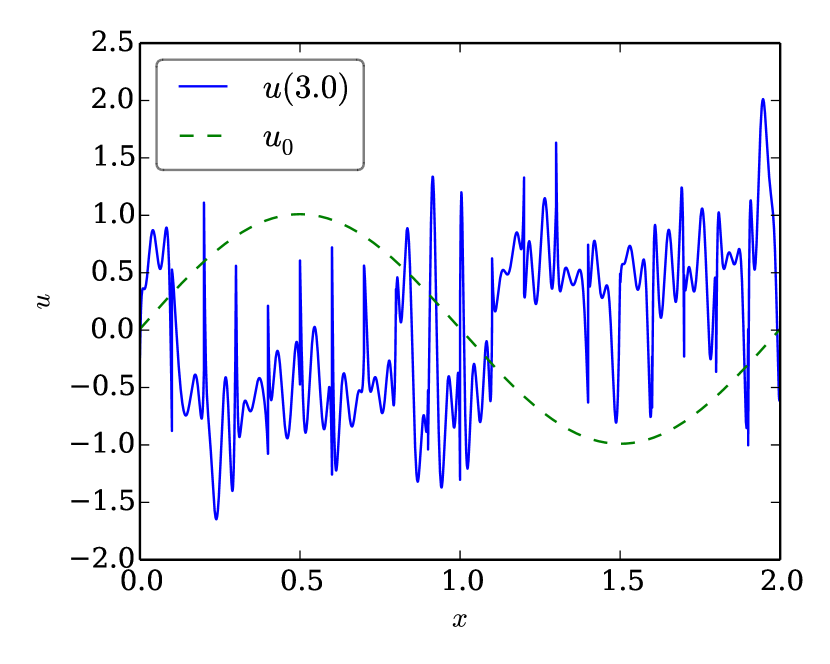
(a) Energy conservative flux.

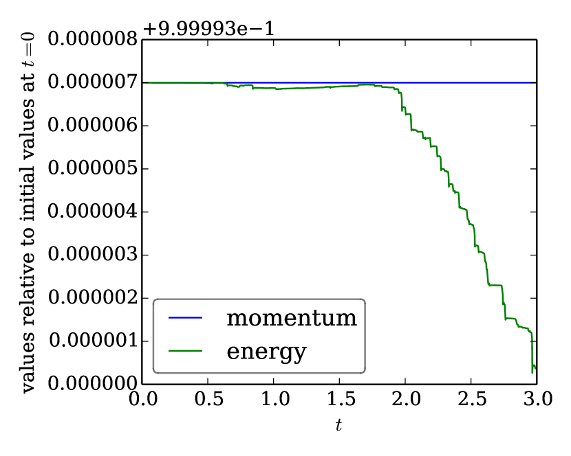
(b) Energy conservative flux.

(c) Local Lax-Friedrichs flux.

(d) Local Lax-Friedrichs flux.

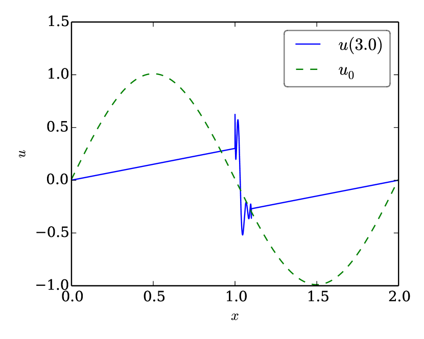
(e) Osher’s flux.

(f) Osher’s flux.

Figure 9: Results of the simulations for Burgers’ equation using an SBP CPR method with correction term for the divergence, 20 elements with a Lobatto-Legendre basis of order 7 and variant numerical fluxes. On the left-hand side, the values of $u(3)$ (blue) and $u(0)=u_{0}$ (green) are shown. On the right-hand site, the discrete momentum $\underline{1}^{T}\underline{\underline{M}}\,\underline{u}$ (blue) and discrete energy $\underline{u}^{T}\underline{\underline{M}}\,\underline{u}$ (green) in the time interval $[0,3]$ are plotted.

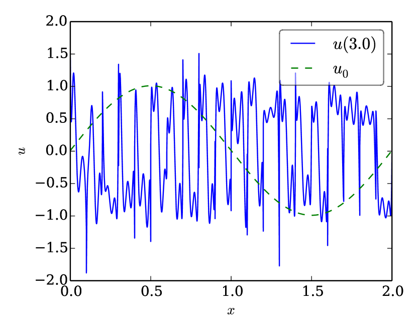
(a) Energy conservative flux.

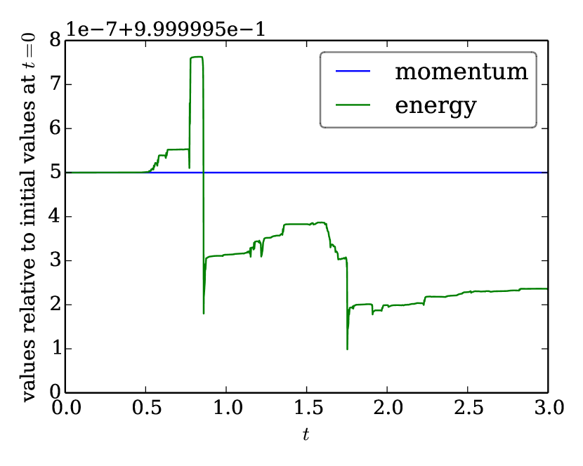
(b) Energy conservative flux.

(c) Local Lax-Friedrichs flux.

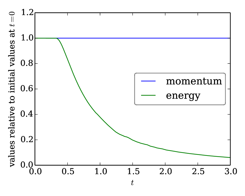
(d) Local Lax-Friedrichs flux.

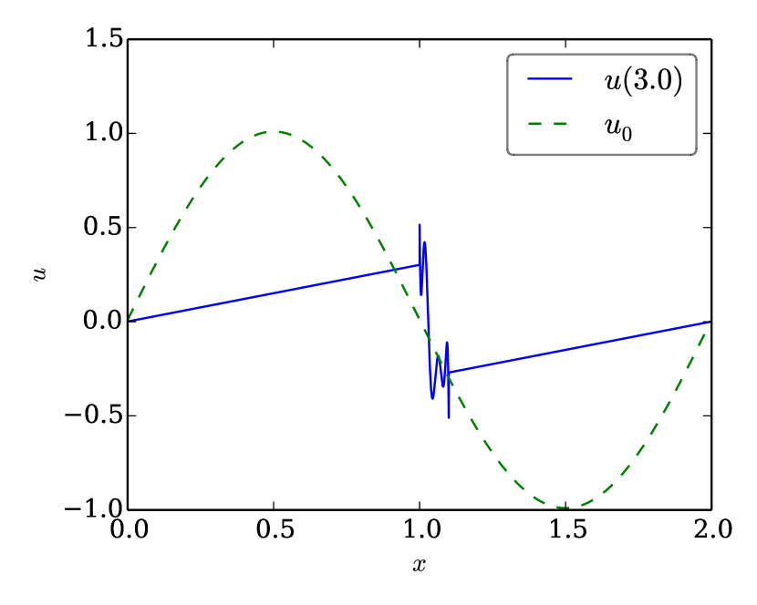
(e) Osher’s flux.

(f) Osher’s flux.

Figure 10: Results of the simulations for Burgers’ equation using an SBP CPR method with correction terms for both the divergence and restriction to the boundary, 20 elements with a Gauß-Legendre basis of order 7 and variant numerical fluxes. On the left-hand side, the values of $u(3)$ (blue) and $u(0)=u_{0}$ (green) are shown. On the right-hand site, the discrete momentum $\underline{1}^{T}\underline{\underline{M}}\,\underline{u}$ (blue) and discrete energy $\underline{u}^{T}\underline{\underline{M}}\,\underline{u}$ (green) in the time interval $[0,3]$ are plotted.

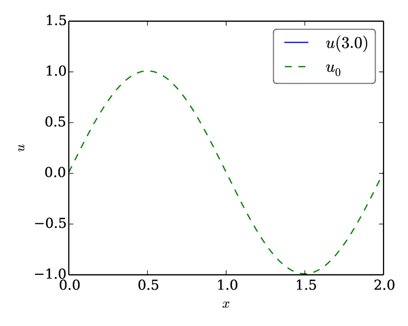
(a) Energy conservative flux.

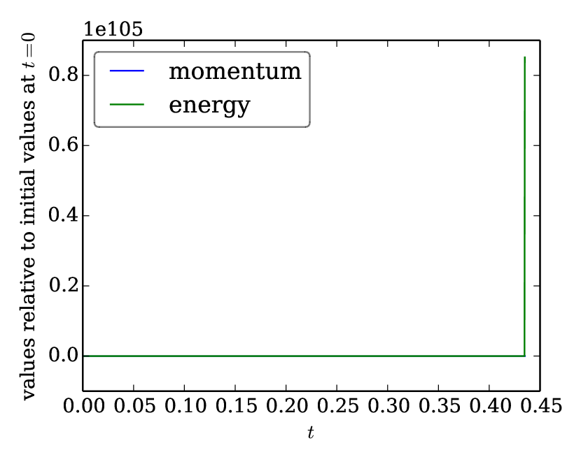
(b) Energy conservative flux.

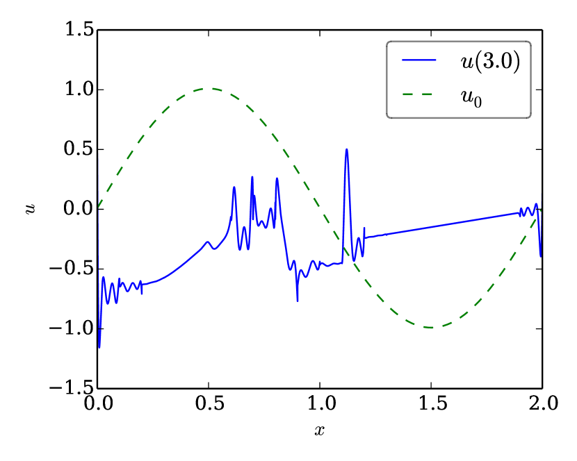
(c) Local Lax-Friedrichs flux.

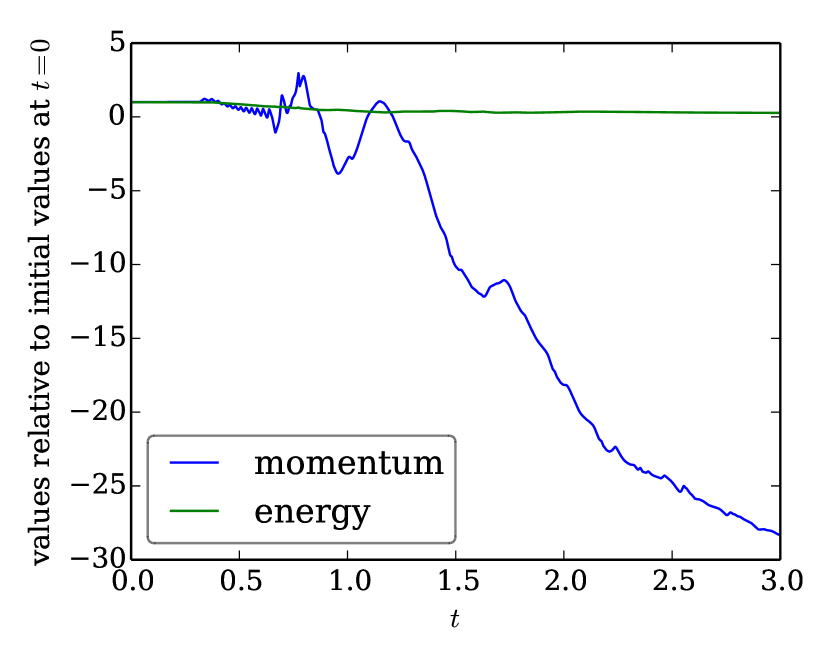
(d) Local Lax-Friedrichs flux.

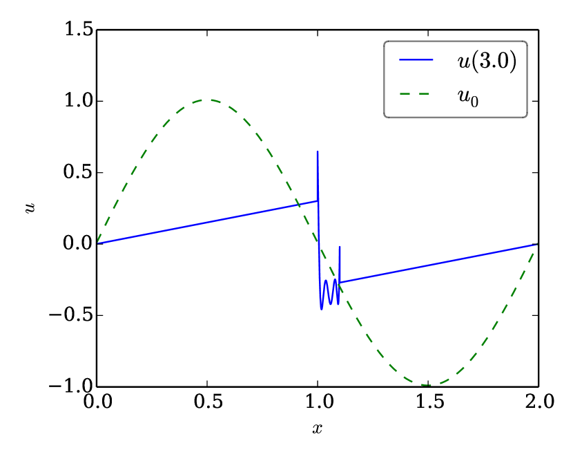
(e) Osher’s flux.

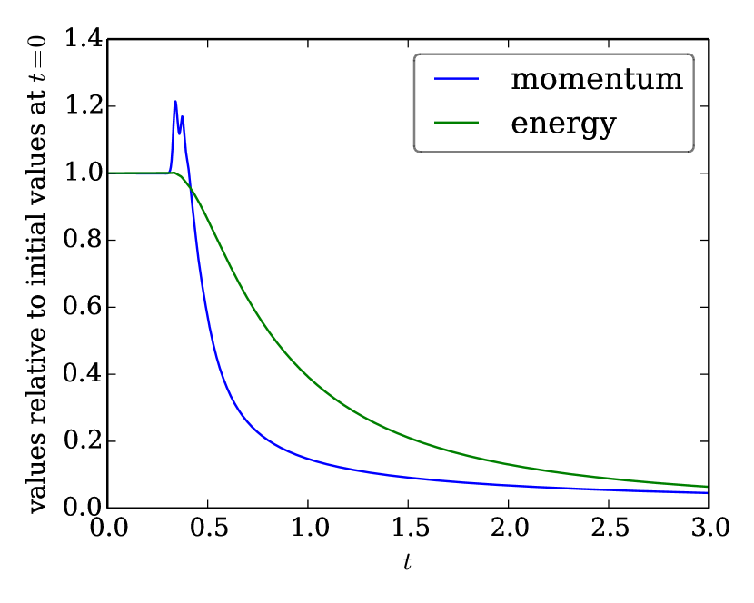
(f) Osher’s flux.

Figure 11: Results of the simulations for Burgers’ equation using an SBP CPR method with correction term only for the divergence, 20 elements with a Gauß-Legendre basis of order 7 and variant numerical fluxes. On the left-hand side, the values of $u(3)$ (blue) and $u(0)=u_{0}$ (green) are shown. On the right-hand site, the discrete momentum $\underline{1}^{T}\underline{\underline{M}}\,\underline{u}$ (blue) and discrete energy $\underline{u}^{T}\underline{\underline{M}}\,\underline{u}$ (green) in the time interval $[0,3]$ are plotted.

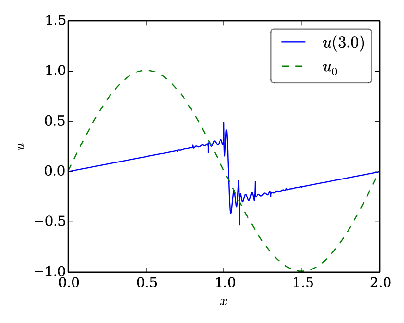
(a) Gauß-Legendre with both correction terms.

(b) Gauß-Legendre with both correction terms.

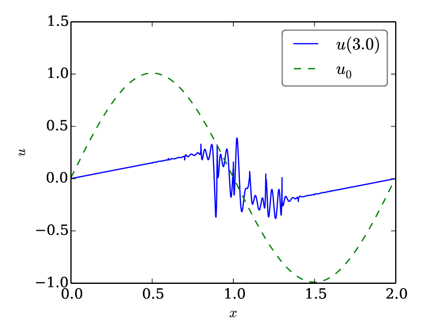
(c) Gauß-Legendre with divergence correction.

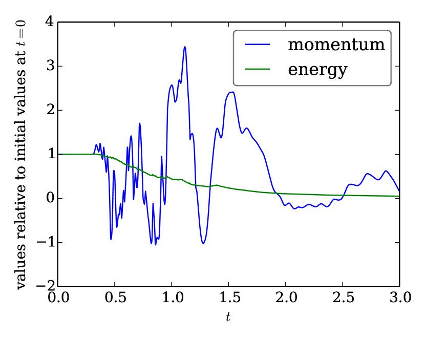
(d) Gauß-Legendre with divergence correction.

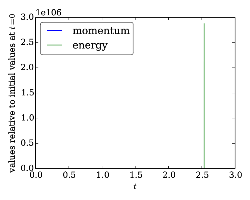
(e) Lobatto-Legendre with divergence correction.

Figure 12: Results for Burgers’ equation using SBP CPR methods with 20 elements, different bases of order 7 and Roe’s flux. In the first row, results for Gauß-Legendre nodes with both correction terms are shown. For the second row, only a divergence correction is used. Results for a Lobatto-Legendre basis with divergence correction are presented in (e). In (a) and (c), the values of $u(3)$ (blue) and $u(0)=u_{0}$ (green) are shown. The discrete momentum $\underline{1}^{T}\underline{\underline{M}}\,\underline{u}$ (blue) and discrete energy $\underline{u}^{T}\underline{\underline{M}}\,\underline{u}$ (green) in the time interval $[0,3]$ are plotted in the other pictures.

(a) Gauß-Legendre with LLF flux.

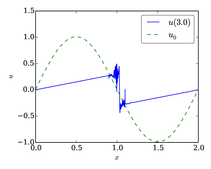
(b) Gauß-Legendre with Osher’s flux.

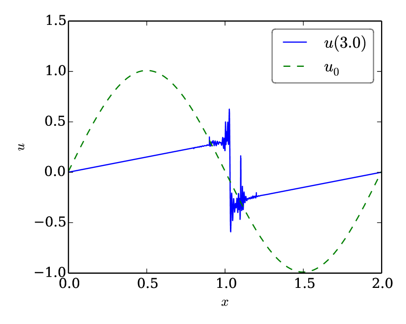
(c) Lobatto-Legendre with LLF flux.

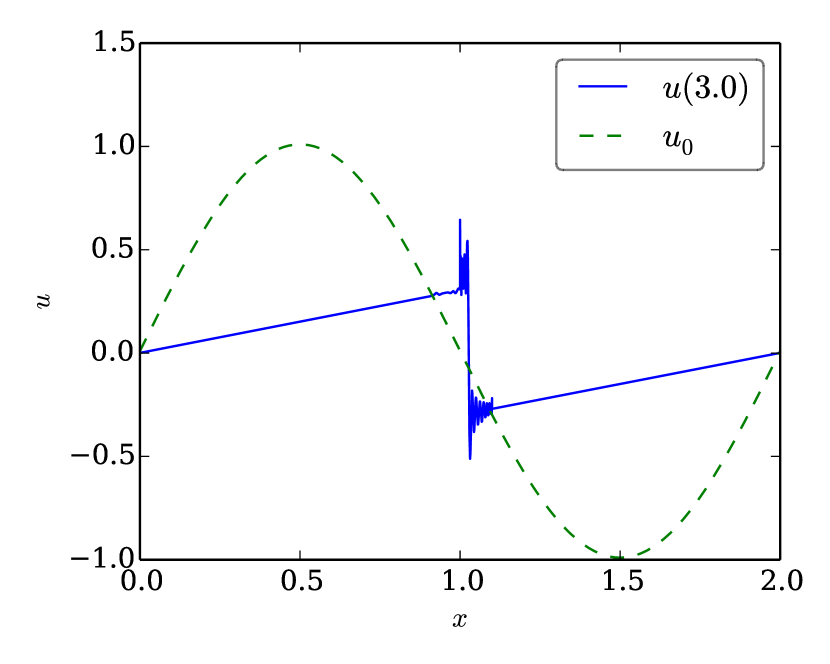
(d) Lobatto-Legendre with Osher’s flux.

Figure 13: Results of the simulations for Burgers’ equation using SBP CPR methods with 20 elements, different bases of order 25 and local Lax-Friedrichs (LLF) or Osher’s flux (on the left- and right-hand side, respectively). In the first row, results for the Gauß-Legendre nodes with correction terms for both divergence and restriction are shown. For the second row, a Lobatto-Legendre basis with a correction for the divergence is used. Each figure shows the values of $u(3)$ (blue) and $u(0)=u_{0}$ (green).

(a) Gauß-Legendre with LLF flux.

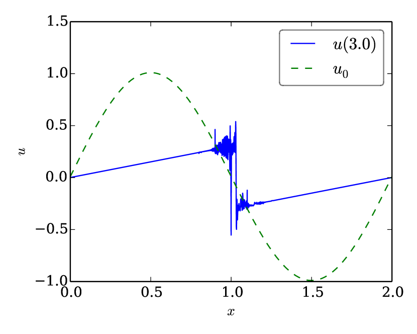
(b) Gauß-Legendre with Osher’s flux.

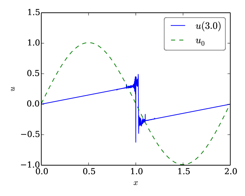
(c) Lobatto-Legendre with LLF flux.

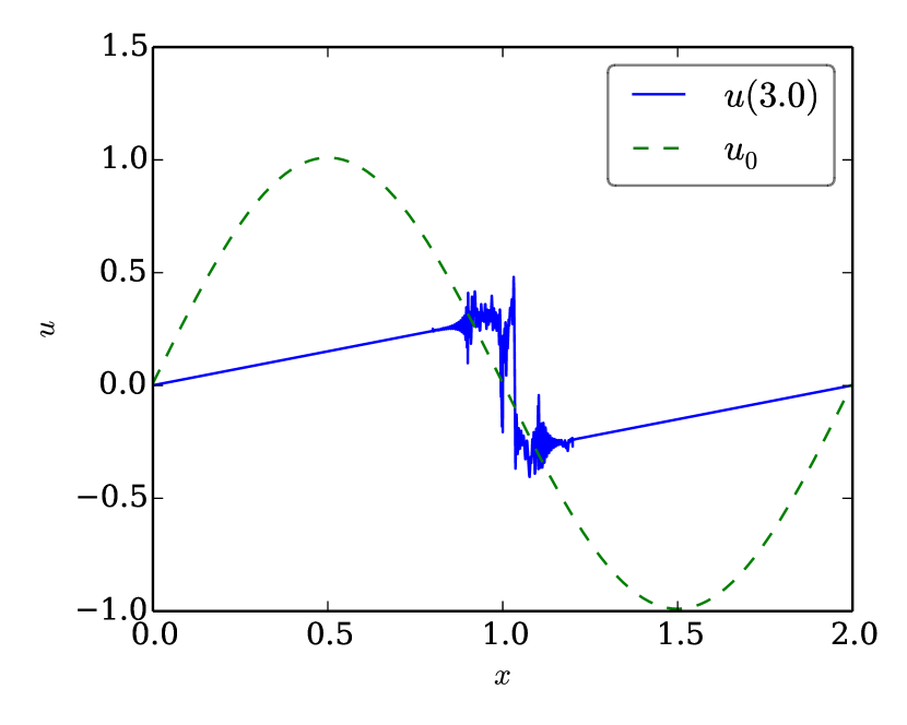
(d) Lobatto-Legendre with Osher’s flux.

Figure 14: Results of the simulations for Burgers’ equation using SBP CPR methods with 20 elements, different bases of order 50 and local Lax-Friedrichs (LLF) or Osher’s flux (on the left- and right-hand side, respectively). In the first row, results for the Gauß-Legendre nodes with correction terms for both divergence and restriction are shown. For the second row, a Lobatto-Legendre basis with a correction for the divergence is used. Each figure shows the values of $u(3)$ (blue) and $u(0)=u_{0}$ (green).

4.5 Extension of the CPR idea

Extending the idea to use a different norm for proving stability does not seem to extend to the corrected formulation of Burgers’ equation, at least in a straightforward way. Indeed, multiplying by $\underline{u}^{T}(\underline{\underline{M}}\,+\underline{\underline{K}}\,)$ instead of $\underline{u}^{T}\underline{\underline{M}}\,$, equation (94) becomes

$$\frac{1}{2}\dfrac{\operatorname{d\!}{}}{\operatorname{d\!}{t}}\mathinner{\!\left\lVert u\right\rVert}_{M+K}^{2}+\frac{1}{3}\underline{u}^{T}(\underline{\underline{M}}\,+\underline{\underline{K}}\,)\underline{\underline{D}}\,\underline{u^{2}}+\frac{1}{3}\underline{u}^{T}(\underline{\underline{M}}\,+\underline{\underline{K}}\,)\underline{\underline{u}}\,\underline{\underline{D}}\,\underline{u}$$ (115)

$$+\underline{u}^{T}(\underline{\underline{M}}\,+\underline{\underline{K}}\,)\underline{\underline{C}}\,(\dots)=0.$$

The standard choice $\underline{\underline{C}}\,=(\underline{\underline{M}}\,+\underline{\underline{K}}\,)^{-1}\underline{\underline{R}}\,^{T}\underline{\underline{B}}\,$ leads to additional terms

$$\frac{1}{3}\underline{u}^{T}\underline{\underline{K}}\,\underline{\underline{D}}\,\underline{\underline{u}}\,\underline{u}+\frac{1}{3}\underline{u}^{T}\underline{\underline{K}}\,\underline{\underline{u}}\,\underline{\underline{D}}\,\underline{u}=\frac{1}{3}\underline{u}^{T}(\underline{\underline{K}}\,\underline{\underline{D}}\,\underline{\underline{u}}\,+\underline{\underline{K}}\,\underline{\underline{u}}\,\underline{\underline{D}}\,)\underline{u}$$ (116)

in comparison with the results for $\underline{\underline{K}}\,=0$. Enforcing stability by requiring $\underline{\underline{K}}\,\underline{\underline{D}}\,\underline{\underline{u}}\,+\underline{\underline{K}}\,\underline{\underline{u}}\,\underline{\underline{D}}\,$ to be skew-symmetric (leading to no further contribution) or symmetric (leading to negative contributions for the rate of change $\frac{1}{2}\dfrac{\operatorname{d\!}{}}{\operatorname{d\!}{t}}\mathinner{\!\left\lVert u\right\rVert}_{M+K}^{2}$ in the positive definite case) implies $\underline{\underline{K}}\,=0$, at least for Gauß-Legendre and Lobatto-Legendre bases of small degree. For brevity, these calculations are not repeated here.

5 Discussion and summary

In this work, the general frameworks of CPR methods and SBP SAT operators are united, leading to a general formulation of semidiscretisations for conservation laws. The linearly stable schemes of Vincent et al. [22, 23] are embedded in this framework, leading to proofs for both conservation and stability in a discrete norm adapted to the method.

Moreover, the DGSEM introduced by Gassner [8] using a skew-symmetric formulation of the conservation law is embedded in this framework. Thus, nonlinear stability results for a special choice of nodal basis (Lobatto-Legendre) can be proven. These results are extended in this work by adapting a new formulation of the conservation law, introducing an additional correction term. In this way, conservation and entropy stability are ensured for more general SBP CPR methods. Especially, a Gauß-Legendre basis not including boundary points is an admissible part of these schemes.

First considerations on the extension of the CPR idea to use different norms in stability proofs in section 4.5 were not successful. Therefore, SBP CPR methods should be used with the canonical correction matrix $\underline{\underline{C}}\,=\underline{\underline{M}}\,^{-1}\underline{\underline{R}}\,^{T}\underline{\underline{B}}\,$ ($\kappa=0$), facilitating stability proofs as in sections 3 and 4. Thus, Gauß-Legendre bases seem to preferable, due to their higher order for quadrature and better approximation qualities, see also Figures 7(e) and 8(e). However, extensions to more complex systems seem to be difficult without relying on boundary nodes. There, Lobatto-Legendre nodes can be advantageous.

Future work will include investigations of different correction matrices (correction functions in the framework of FR methods) ensuring entropy stability for nonlinear conservation laws, since the straightforward extension of the linear case seems not to be possible. Additionally, fully discrete schemes will be investigated, incorporating the influence of different time discretisations into the hitherto obtained results. Therefore, special attention must be paid to the described volume term.

Of course, a straightforward application of SBP CPR schemes in multiple dimensions using tensor products is possible. Future work will focus on inherently multi-dimensional SBP CPR bases for both tensor product type elements and simplices, using the new formulation of these schemes.

References

- [1] Y. Allaneau and A. Jameson. Connections between the filtered discontinuous Galerkin method and the flux reconstruction approach to high order discretizations. Computer Methods in Applied Mechanics and Engineering, 200(49):3628–3636, 2011.
- [2] P. Castonguay, P. E. Vincent, and A. Jameson. A new class of high-order energy stable flux reconstruction schemes for triangular elements. Journal of Scientific Computing, 51(1):224–256, 2012.
- [3] P. Castonguay, D. Williams, P. E. Vincent, and A. Jameson. Energy stable flux reconstruction schemes for advection–diffusion problems. Computer Methods in Applied Mechanics and Engineering, 267:400–417, 2013.
- [4] D. De Grazia, G. Mengaldo, D. Moxey, P. E. Vincent, and S. Sherwin. Connections between the discontinuous galerkin method and high-order flux reconstruction schemes. International journal for numerical methods in fluids, 75(12):860–877, 2014.
- [5] D. C. D. R. Fernández, P. D. Boom, and D. W. Zingg. A generalized framework for nodal first derivative summation-by-parts operators. Journal of Computational Physics, 266:214–239, 2014.
- [6] D. C. D. R. Fernández, J. E. Hicken, and D. W. Zingg. Review of summation-by-parts operators with simultaneous approximation terms for the numerical solution of partial differential equations. Computers & Fluids, 95:171–196, 2014.
- [7] T. C. Fisher, M. H. Carpenter, J. Nordström, N. K. Yamaleev, and C. Swanson. Discretely conservative finite-difference formulations for nonlinear conservation laws in split form: Theory and boundary conditions. Journal of Computational Physics, 234:353–375, 2013.
- [8] G. J. Gassner. A skew-symmetric discontinuous Galerkin spectral element discretization and its relation to SBP-SAT finite difference methods. SIAM Journal on Scientific Computing, 35(3):A1233–A1253, 2013.
- [9] G. J. Gassner. A kinetic energy preserving nodal discontinuous Galerkin spectral element method. International Journal for Numerical Methods in Fluids, 76(1):28–50, 2014.
- [10] G. J. Gassner and D. A. Kopriva. A comparison of the dispersion and dissipation errors of Gauss and Gauss-Lobatto discontinuous Galerkin spectral element methods. SIAM Journal on Scientific Computing, 33(5):2560–2579, 2011.
- [11] G. J. Gassner, A. R. Winters, and D. A. Kopriva. A well balanced and entropy conservative discontinuous Galerkin spectral element method for the shallow water equations. Applied Mathematics and Computation, 272:291–308, 2016.
- [12] J. E. Hicken and D. W. Zingg. Summation-by-parts operators and high-order quadrature. Journal of Computational and Applied Mathematics, 237(1):111–125, 2013.
- [13] H. Huynh. A flux reconstruction approach to high-order schemes including discontinuous Galerkin methods. AIAA paper, 4079:2007, 2007.
- [14] H. Huynh, Z. J. Wang, and P. E. Vincent. High-order methods for computational fluid dynamics: A brief review of compact differential formulations on unstructured grids. Computers & Fluids, 98:209–220, 2014.
- [15] A. Jameson. A proof of the stability of the spectral difference method for all orders of accuracy. Journal of Scientific Computing, 45(1-3):348–358, 2010.
- [16] A. Jameson, P. E. Vincent, and P. Castonguay. On the non-linear stability of flux reconstruction schemes. Journal of Scientific Computing, 50(2):434–445, 2012.
- [17] D. A. Kopriva and G. J. Gassner. On the quadrature and weak form choices in collocation type discontinuous Galerkin spectral element methods. Journal of Scientific Computing, 44(2):136–155, 2010.
- [18] D. A. Kopriva and G. J. Gassner. An energy stable discontinuous Galerkin spectral element discretization for variable coefficient advection problems. SIAM Journal on Scientific Computing, 36(4):A2076–A2099, 2014.
- [19] M. Svärd and J. Nordström. Review of summation-by-parts schemes for initial–boundary-value problems. Journal of Computational Physics, 268:17–38, 2014.
- [20] E. F. Toro. Riemann solvers and numerical methods for fluid dynamics: a practical introduction. Springer Science & Business Media, 2009.
- [21] P. E. Vincent, P. Castonguay, and A. Jameson. Insights from von Neumann analysis of high-order flux reconstruction schemes. Journal of Computational Physics, 230(22):8134–8154, 2011.
- [22] P. E. Vincent, P. Castonguay, and A. Jameson. A new class of high-order energy stable flux reconstruction schemes. Journal of Scientific Computing, 47(1):50–72, 2011.
- [23] P. E. Vincent, A. M. Farrington, F. D. Witherden, and A. Jameson. An extended range of stable-symmetric-conservative flux reconstruction correction functions. Computer Methods in Applied Mechanics and Engineering, 296:248–272, 2015.
- [24] Z. Wang and H. Gao. A unifying lifting collocation penalty formulation including the discontinuous Galerkin, spectral volume/difference methods for conservation laws on mixed grids. Journal of Computational Physics, 228(21):8161–8186, 2009.
- [25] D. Williams, P. Castonguay, P. E. Vincent, and A. Jameson. Energy stable flux reconstruction schemes for advection–diffusion problems on triangles. Journal of Computational Physics, 250:53–76, 2013.
- [26] F. D. Witherden and P. E. Vincent. An analysis of solution point coordinates for flux reconstruction schemes on triangular elements. Journal of Scientific Computing, 61(2):398–423, 2014.
- [27] F. D. Witherden and P. E. Vincent. On the identification of symmetric quadrature rules for finite element methods. Computers & Mathematics with Applications, 69(10):1232–1241, 2015.
- [28] M. Yu and Z. Wang. On the connection between the correction and weighting functions in the correction procedure via reconstruction method. Journal of Scientific Computing, 54(1):227–244, 2013.