Super-resolving multiresolution images with band-independant geometry of multispectral pixels

Abstract

A new resolution enhancement method is presented for multispectral and multi-resolution images, such as these provided by the Sentinel-2 satellites. Starting from the highest resolution bands, band-dependent information (reflectance) is separated from information that is common to all bands (geometry of scene elements). This model is then applied to unmix low-resolution bands, preserving their reflectance, while propagating band-independent information to preserve the sub-pixel details. A reference implementation is provided, with an application example for super-resolving Sentinel-2 data.

INRIA Bordeaux Sud-Ouest / Geostat, 200 avenue de la vieille tour, 33405 Talence, France

I Introduction

I-A Context and state of art

Earth Observation missions typically operate at medium to low resolution ranges in order to favor both larger satellite swath and better temporal revisit of the same site (e.g. 3-4 days over Europe for the Sentinel-2 Satellite series). For each acquisition, optical constraints furthermore often restrict that only some spectral bands have maximal resolution. For example, a common case is to compensate the smaller pixel size of the higher spatial resolution bands (e.g. 10m/pixel) by capturing light over a larger spectrum range (e.g. 4 large bands in the red, green, blue and near infrared for Sentinel-2). The limit case being a single high-resolution panchromatic band (Pleiades, Spot, Landsat…). Narrower spectral bands, invaluable for specific measurements (e.g. chlorophyll or water vapor absorbtion wavelengths) are then provided at lower resolution (e.g. 20m/pixel and 60m/pixel for Sentinel-2). Yet, this trade-off on spectral and spatial resolutions may become a limiting factor for many Earth Observation applications, for example for getting accurate land cover classification at the highest resolution [1]. Some techniques have thus been devised in order to propagate the high-resolution spatial details to the lower-resolution dedicated bands while preserving their spectral content. These can be sorted along the following categories:

– Probabilistic [7, 8]: The spectral information in each sub-pixel of an original low-resolution pixel is determined by maximizing a probabilistic model, constrained by the observed data at all bands and resolutions (possibly including the panchromatic band). A Bayesian formulation can be choosen to represent this constraint which, provided this does not becomes intractable, allows hyperparameters to be set according to prior knowledge.

– Sensor-based: If the sensor has a known point spread function (PSF), then deconvoluting it enhances the resolution of the acquired images [9]. But the PSF for many satellites can only be estimated empirically (Sentinel-2, Spot-5, Landsat-8 [1]). When that is the case, limits on sub-pixel detection can be established [1].

– Learning-based: These methods exploit local patterns in the low-resolution images, and propagate these features (e.g. edges) to infer the higher resolution image [10]. Many models may be used to “learn” the features: neural network [11], example-based [12] with kernel ridge regression [13], deep learning [14] and more references therein, including for cross-image learning. These methods can be applied for single image resolution enhancement, possibly with different channels (typically red, green, blue [14]). Filling details from learned (or duplicated) texture features might be very good to produce visually plausible results [12]. Their main problem, similar to in-painting with image-based examples [15], is that “hallucinated” [10] details do not necessarily correspond to true higher-resolution objects (esp. with non-local or cross-image features) and then become misleading pixels for land monitoring purposes.

– Scaling laws: Instead of learning local patterns, this method learns multi-scale relationships in the data such as local power laws between spatial extent and band values [18]. Such scaling laws are inferred from data above the aquisition resolution but, assuming the same laws remain valid below that resolution, these can then be used to infer sub-pixels of the original image. Very good results have been obtained with such methods for turbulent oceanic data [19], where energy cascades translates to power laws spanning multiple decades. However, for land monitoring purposes, usually no such physical interpretation can be found: for example a mixture of trees, houses and roads in a peri-urban environment is not locally scale-invariant.

– Frequency representations: Working in the frequency domain, whether with Fourier methods or using wavelet decompositions. An idea is to upsample the low-frequencies (e.g. with a bicubic filter) and preserve the high frequency components. Unfortunately, natural images are not statistically consistent: knowledge that there is a tree (or road, house…) a few hundred meters away (i.e. the wavelet support size) does not help subdivide a local pixel into its higher-resolution components.

– Panchromatic sharpening [2]: Using a very wide band with high-resolution in order to compensate the lower resolution of narrow bands. Multiple variants exist, from a simple renormalization of the multispectral bands [3] to more advanced unmixing techniques which estimate the contribution of each spectral band to the panchromatic one [4], possibly with pre-processing steps designed to uncorrelate each component [5, 2], or using angular spaces such as the hyperspherical color space [6].

The advantages of panchromatic sharpening are its efficiency, and its applicability even when only a single high-resolution band is acquired. Many observation satellites thus include a panchromatic band, but some do not (e.g. ESA’s Sentinel-2 series, specifications given in Appendix). In the absence of such a band, and given the inadequacies of the other methods presented above, another solution is needed.

I-B Super-resolution of multispectral images in the absence of a panchromatic band

In a multispectral measurement system, each pixel in a band $B$ captures the light intensity over some part of the spectrum, according to some sensor sensitivity distribution $s_{B}(\lambda)$ for each wavelength $\lambda$: $B(x,y)=\int s_{B}(\lambda)I(\lambda,x,y)d\lambda$. The light intensity $I$ is reflected at wavelength $\lambda$ by the pixel surface between $x+r_{B}$ and $y+r_{B}$, where $r_{B}$ is the square pixel resolution of band $B$. Larger pixels thus collect more light and may be necessary for some bands with narrow $s_{B}$ spectral support. This very simplified model ignores many sources of optical distortions and the post-processing from satellite geometry to square pixels, but these effects are irrelevant in the context of this section.

When a panchromatic band $P$ is available, light is collected over a wide spectrum support : $s_{P}(\lambda)\neq 0$ for a large range of wavelengths $[\lambda_{Pmin},\lambda_{Pmax}]$, usually covering all other bands $\lambda_{Pmin}\leq\lambda_{Bmin}\leq\lambda_{Bmax}\leq\lambda_{Pmax}$. Collecting more light spectrally allows to reduce the pixel size $r_{P}<r_{B}$ while still maintaining a minimal intensity to trigger the panchromatic sensor. Each band pixel $B(x,y)$ thus covers an area with multiple panchromatic pixels $P(x+i*r_{P},\,\,y+j*r_{p})$ for $i,j$ indices depending on the band resolution $r_{B}$. The total light reaching the sensor for $B(x,y)$ may thus be related to the values of each sub-pixels $P(x+i*r_{P},\,\,y+j*r_{p})$ by a function involving both spatial and spectral components. Panchromatic sharpening methods attempt to unmix this total light contribution by defining $B(x,y)=f(H(x+i*r_{p},\,\,y+i*r_{p}))$, where $H$ is a high-resolution version of band $B$. $f$ is a coarse-graining function, for example $f=\sum_{i,j}$ in the simplest case. More elaborated functions may be necessary, for example when combining both panchromatic sharpening and atmospheric corrections. The relations between $s_{P}(\lambda)$ and $s_{B}(\lambda)$ are used in order to further constrain $H$ with values of $P$ at the same pixel locations.

Unfortunately, for Sentinel-2 images, there is no panchromatic band. Methods using such bands, cited in the previous Section, are thus not directly useable. An idea would be to create a virtual $P$ band by combining the four high-resolution bands $B^{10}$ at 10m/pixel, and then apply pansharpening methods for bands at 20m/pixel and 60m/pixel. But combining blue, green, red, and infrared bands into a virtual intensity would result in a virtual $s_{P}(\lambda)$ that only covers the original $s_{B^{10}}(\lambda)$, and thus prone to spectral artifacts for super-resolving the values of the other bands $B^{20}$ and $B^{60}$. Similarly, spatial details in that hypothetical $P$ band would depend on how that virtual $P$ is constructed from other $B^{10}$ bands (in particular, how infrared details are fused with visible light details).

In the absence of a real panchromatic band, a better idea is to design a new method that:

– Explicitely encodes geometric details from available high-resolution bands, as pixel properties independent from their reflectance;

– Preserves the spectral content of each low-resolution band independently from the geometry.

The next sections introduce one method for acheiving this, with direct applicability to Sentinel-2 images. The method presented below works with only local information, hence it is not subject to the non-local effects mentionned in the previous section. The method relies on the observation that the proportion of objects of the same nature within a pixel area (e.g. 30% urban area, 70% trees), is a physical property of that pixel and therefore independent of the spectral band. Only the reflectance of these objects may change from band to band. Moreover, there is no reason why pixel boundaries would match natural object boundaries. The method thus identifies generic “shared” information between adjacent pixels, then commonalize the geometric aspects of these shared values across bands. High resolution bands are used to separate band-independent information from band-dependant reflectance. The geometric information is then used to unmix the low-resolution pixels, while preserving their overall reflectance.

Section II presents the super-resolution problem and Section III details how that problem is addressed by the model introduced in this paper. Section IV indicates how to quantify the results quality, and section V shows super-resolution results for three different types of regions of interest (coastal, urban, agricultrural). Results are followed by a discussion in Section VI, which also demonstrates the influence of each step of the algorithm.

II Problem description

II-A Super-resolution formulation

Figure 1: Introducing the indexing and the relations between the low and high resolution pixels, for the simple case of doubling the resolution. The grayed lines indicate boundaries from Fig. 2, for ease of interpretation.

Let $L$ be an observed low resolution image with $N_{x}/2$ columns and $N_{y}/2$ rows. We consider the problem of finding a high resolution image $H$ with $N_{x}$ columns and $N_{y}$ rows. Each low resolution pixel $L_{x/2,y/2}$ thus corresponds to $4$ high resolution pixels, as depicted in Fig. 1. Averaging these pixels should give the original observed low-resolution pixel back:

$$L_{x/2,y/2}=\frac{1}{4}\left(H_{x,y}+H_{x+1,y}+H_{x,y+1}+H_{x+1,y+1}\right)$$ (1)

Images remotely sensed from satellites are subject to multiple transforms (including atmospheric corrections [24]) before being released as a useable product. These transforms are out of scope of the present document but may introduce correlations between high-resolution pixels (e.g. due to scattering), hence should be applied before (or integrated to) super-resolution. Similarly, known PSF [9] should be deconvoluted in addition to the method presented below. In any case, Eq. 1 ensures that down-sampling by averaging the high-resolution solution will recover the observations.

Eq. 1 is undetermined, with 3 free parameters per low resolution pixel. Some extra constraints are needed, which are extracted from available high-resolution data bands.

II-B Shared information between neighbor pixels

Figure 2: Values $S$ shared between neighbor pixels, and how these are combined by weights $W$ to form the high-resolution pixels. Compare with the boundaries from Fig. 1, indicated as grayed lines for ease of interpretation. Shared values span over multiple pixels by definition. These values represent the reflectance of elements that are common to the spanned pixels. Weights are internal to each pixel and represent the proportion of these elements within the pixel. Weights are thus independant of the spectral band.

Natural objects do not fall exactly on pixel boundaries. Therefore, some content is shared between nearby pixel values. This shared information is explicitly defined as in Fig. 2, left. For example, $S_{x+1,y+1}$ is the reflectance corresponding to the shared part between high-resolution pixels $H_{x,y}$, $H_{x+1,y}$, $H_{x,y+1}$ and $H_{x+1,y+1}$ (compare Fig. 1 and Fig. 2). This particular element is fully within the observed low-resolution pixel $L_{x/2,y/2}$. Other shared values may span multiple low-resolution pixels. With this notation, there are $\left(N_{x}+1\right)\times\left(N_{y}+1\right)$ spatially shared values $S$. These located at the image boundaries, or which would span invalid pixels such as in the case of sensor failure, are simply not commonalized and effectively remain internal to the valid pixels. All shared values are expressed in reflectance units and constrained to the range of their respective band.

In remote sensing, the reflectance of each pixel is often considered to be a linear mix [20] of the reflectances of its constituents (e.g. a mix of vegetation and soil). Assuming the shared values correspond to unknown constituents spanning over pixel boundaries, and using this linear mixing model, the proportion of each shared value that is present in each pixel is thus determined by weights that are specific to that pixel (Fig. 2, right). This leads to the following mixing equation for the shared values and the weights:

$$H_{x,y}= W_{x,y,0}S_{x,y}+W_{x,y,1}S_{x+1,y}$$ (2)

$$+ W_{x,y,2}S_{x,y+1}+W_{x,y,3}S_{x+1,y+1}$$

With the following constraints:

$$\sum_{k=0}^{3}W_{x,y,k}=1$$ (3)

$$W_{x,y,k}\geq 0\,\,\,\forall k\in[0\ldots 3]$$ (4)

III Solving the super-resolution problem

III-A Separating band-specific information from information common to all bands

The proportion of mixed elements within a pixel (e.g. 20% road / 80% vegetation) is a physical property of that pixel, but the reflectance of each element depends on the spectral band at which it is observed. Therefore, the weights are common to all bands, while shared values are band-dependant. Weights encode the geometric consistency of pixels accross bands. Shared values encode the spatial consistency of nearby pixels. The high-resolution data are used to fit the full mixing model, containing both weights and shared values. This step is presented below. The next section addresses how to un-mix low-resolution bands in order to produce the super-resolution result, reusing the weights fit from the high-resolution bands.

Starting from an observed high-resolution band $H^{o}$, a down-sampled version $L^{d}$ of the data is created with Eq. 1. The best mixing model is estimated by minimizing the difference between: a) the observed pixel values $H^{o}$, and b) the resolution-enhanced values $H^{r}$ computed from the down-sampled data $L^{d}$. Let us subscript data specific to each band with an additional index $\beta$. Thus, $L^{d}$, $H^{o}$, $H^{r}$ and $S$ are subscripted, but not the weights $W$. Solving this first problem is a constrained minimization, for $k=0\ldots 3$, and $\beta\in\mathcal{H}$ the set of high-resolution bands:

$$\left\{S^{opt},W^{opt}\right\}=\textrm{argmin}\sum_{\beta\in\mathcal{H}}\sum_{x,y}\left\|H_{\beta,x,y}^{o}-H_{\beta,x,y}^{r}\right\|^{2}$$ (5)

with each $H_{\beta,x,y}^{r}$ term given by Eq. 2. An iterative solver [21] is used for constrained least squared error optimization, allowing Eq. 3 to be enforced by a reparametrization and Eq. 4 by soft boundaries (a reference implementation is provided, link given in appendix). Initial weights for the iterative algorithm are set to $\frac{1}{4}$ (i.e. equal influence to all shared values, see Fig. 2, left). The initial shared values $S_{\beta}^{ini}$ are computed by averaging each high-resolution pixel $H_{\beta}^{o}$ that partially covers $S_{\beta}^{ini}$ in Fig. 2. For example, $S_{\beta,x+1,y+1}^{ini}=\frac{1}{4}\left(H_{\beta,x,y}^{o}+H_{\beta,x+1,y}^{o}+H_{\beta,x,y+1}^{o}+H_{\beta,x+1,y+1}^{o}\right)$.

At the end of this step, both shared values $S_{\beta}^{opt}$ between high-resolution pixels, and weights $W^{opt}$ common to all bands, are available.

III-B Estimating shared values from low-resolution data

Shared values $S^{opt}$ are found by optimization on high-resolution data, so they cannot be estimated directly on the low-resolution bands with the above procedure. Instead, the relation between $S^{opt}$ and nearby low-resolution pixels can be learned from downsampled high-resolution bands $L^{d}$. That relation is also expressed as a geometric property common to all bands, so it can be used in order to produce a first estimate $S^{fit}$ for the low-resolution bands. More specifically, a second set of mixing coefficients $V$ is built in order to fit $S_{\beta,x,y}^{opt}$ from low-resolution pixels $L_{\beta,n}^{d}$ at nearby locations $n\in\mathcal{N}(x,y)$. See Fig. 3, with $\mathcal{N}$ being either the corner, middle or inner variant depending on the position of $(x,y)$ with respect to the low-resolution reference pixel.

Figure 3: Low-resolution neighborhoods for high-resolution shared values. Depending on the location of the shared value with respect to the center reference pixel (corner, middle, inner), the neighborhood consists of either 4, 6 or 9 low-resolution pixel locations. Other corner and middle locations are deduced by a rotation of the pattern.

These neighborhoods hopefully capture local features (e.g. edges), in the form of up to $9$ coefficents $v_{x,y,n}$ for each high-resolution pixel $(x,y)$ in the image:

$$V=\textrm{argmin}\sum_{\beta\in\mathcal{H}}\sum_{x,y}\left\|S_{\beta,x,y}^{opt}-\sum_{n\in\mathcal{N}\left(x,y\right)}v_{x,y,n}L_{\beta,n}^{d}\right\|^{2}$$ (6)

With this global optimization, the set of coefficients $V$ encodes how the shared values are related to their low-resolution neighborhood, independently of the spectral band. They are fit from the high-resolution bands, and then propagated to the low-resolution bands $b\in\mathcal{L}$ in order to provide a first estimate $S^{fit}$ for the shared values in each band $b$:

$$S_{b,x,y}^{fit}=\sum_{n\in\mathcal{N}\left(x,y\right)}v_{x,y,n}L_{b,n}$$ (7)

The fit from Eq. 6 is rarely perfect and values $S_{\beta,x,y}^{fit}=\sum_{n\in\mathcal{N}\left(x,y\right)}v_{n}L_{\beta,n}^{d}$ can also be computed for the original high-resolution bands. The ratios $q_{\beta,x,y}=S_{\beta,x,y}^{opt}/S_{\beta,x,y}^{fit}$ are then exploited in order to mimick the panchromatic sharpening method in [3], but using the multiple high-resolution bands instead. For Sentinel-2, no panchromatic band is available to encompass the spectrum of all low-resolution bands. An idea is to empirically replace the panchromatic band by a combination of high-resolution bands. Problems mentionned in Section I-B are adressed by weighting bands that yield close spectral responses for the shared values. For each low resolution band $b\in\mathcal{L}$, and for each shared value, a normalized proximity measure is defined as $p_{b,\beta,x,y}=|S_{b,x,y}^{fit}-S_{\beta,x,y}^{fit}|/\max_{\alpha}|S_{b,x,y}^{fit}-S_{\alpha,x,y}^{fit}|$, where the normalization is performed by using the maximum discrepancy over all high resolution bands $\alpha\in\mathcal{H}$. Combining the high-resolution sharpening ratios is then performed by geometric averaging, using these proximity measures as weighting factors:

$$\bar{q}_{b,x,y}=\exp\left(\left(\sum_{\beta}p_{b,\beta,x,y}\log q_{\beta,x,y}\right)/\sum_{\beta}p_{b,\beta,x,y}\right)$$ (8)

This overall average sharpening ratio is used as a prefactor for setting corrected shared values $S_{b,x,y}^{cor}=\bar{q}_{b,x,y}S_{b,x,y}^{fit}$ for the low resolution bands. Having now estimated high-resolution shared values for the low-resolution bands, it is a simple matter of combining these $S_{b,x,y}^{cor}$ with the weights $W$ by applying Eq. 2, in order to produce super-resolved pixels. A final rescaling of these $H_{b,x,y}^{r}$ is performed so as to ensure reflectance is preserved (Eq. 1).

III-C Super-resolving 60m/pixel bands

Figure 4: Introducing the indexing and the relations between the low and high resolution pixels, for the case of tripling the resolution. The shared values between pixels are also indicated. Weights are still internal to each high-resolution pixel with exactly the same structure as in Fig. 2, right.

In this setup, each low-resolution pixel corresponds to 36 values at 10m/pixel. Solving this directly is not tractable, but an indirect solution with an intermediate step is feasible:

– In a first pass, a 60m/pixel band is super-resolved to 20m/pixel. There are then 9 sub-pixels to infer for each low-resolution pixel, with 8 free parameters (Fig. 4 and Eq. 9 below). However, there are also 10 bands at 20m/pixel (including the 4 bands at 10m/pixel, downsampled). These provide enough constraints for the inference of weight values, common to all these bands, computed with a modified version of the method presented below.

– In a second pass, the 20m/pixel solution from the first pass is super-resolved down to 10m/pixel with the method described in the previous sections.

Adapting the above notation to the 9 sub-pixels problem, in this section the low resolution bands are $b\in\mathcal{L}$ at 60m/pixel, while the high resolution bands $\beta\in\mathcal{H}$ consist of the 20m/pixel bands (either original or down-sampled from 10m/pixel). Preserving the reflectance imposes (Fig. 4):

$$L_{b,x/3,y/3}=\frac{1}{9}\sum_{i,j=0}^{2}H_{b,x+i,y+j}^{r}$$ (9)

$H_{b}^{r}$ is the intermediate super-resolution solution at 20m/pixel for band $b$. Fig. 4 also shows the relation between $L_{b}$, the high-resolution pixels $H_{b}^{r}$ and the shared values. With this convention, the weights $W$ follow exactly the same $(x,y)$ pattern with respect to $S$ and $H$ as in Fig. 2, right. The first step of the method, the estimation of both $W$ and $S$ with all available high-resolution bands, is thus also the same as above. All 10 bands $\beta\in\mathcal{H}$ are used as constraints for Eq. 5.

A difference lies in estimating $V$ from nearby pixels. There are still four neighborhood patterns of the “corner” type (see Fig. 3), for shared values$S_{x,y}$, $S_{x+3,y}$, $S_{x,y+3}$ and $S_{x+3,y+3}$. But there are now two “middle” neighborhood patterns for each side of the lower-resolution pixel (e.g. $S_{x+1,y}$, $S_{x+2,y}$), as well as four “inner” neighborhood patterns instead of one (see Fig. 4, right). With these definitions, Eq. 6 is solved as before. Averaging the sharpening ratios now involves all 10 bands $\beta\in\mathcal{H}$ (instead of 4 in the previous section), but this does not change Eq. 8. Thus, solving the 60m$\rightarrow$20m super-resolution problem is performed with very little adaptation.

Once computed, the intermediate solutions at 20m/pixel are further processed by a final 20m$\rightarrow$10m super-resolution step, as described in the above sections.

IV Performance assessement

Quantitative measures are needed in order to evaluate the quality of the super-resolution. Typical quantifiers [22, 23] include :

– The quality index $Q(x,y)=\frac{4\cdot cov(x,y)\cdot mean(x)\cdot mean(y)}{\left(var(x)+var(y)\right)\left(mean(x)^{2}+mean(y)^{2}\right)}$ between an image $x$ and an image $y$.

– The normalized mean squared error $ERGAS(x,y)=100R\sqrt{\frac{1}{N}\sum_{i=1}^{N}\frac{MSE(x_{i},y_{i})}{mean(x_{i})}}$, where $N$ is the number of bands, $x$ is the reference image, and $y$ is the image to be tested.

– The spectral angle $SAM=\textrm{arccos}\left(\frac{x\cdot y}{\left\|x\right\|\left\|y\right\|}\right)$, considering the $x$ and $y$ images as vectors. $SAM$ is given in degrees in the next Section.

– When a panchromatic band $P$ is available, the quality with no reference $QNR=\left(1-D_{\lambda}\right)^{\alpha}\left(1-D_{s}\right)^{\beta}$ can be used, where $D_{\lambda}$ is a spectral distortion index and $D_{s}$ is a spatial distortion index. But $D_{s}$ depends on $P$ so, in the present case with no panchromatic band available, $QNR$ is not useable.

In the following sections, $Q$, $ERGAS$ and $SAM$ are computed. The typical methodology for using these quantifiers is to down-sample an image, super-resolve this down-sampled image back to the original resolution, and compare with the original data. Typically, the highest-resolution bands are used for downsampling/super-resolution. But, due to the way super-resolution is performed in this paper, downsampling 10m bands to 20m and super-resolving them back for comparison is not acceptable. Indeed, that very step is already included as part of the optimization in Eq. 5. Moreover, shared details coming from all original 10m bands are taken into account in Eqs. 6-8. Hence, a test that uses these same 10m bands as a basis for comparison wouldn’t be fair. The method is thus adapted as follows :

– The 20m bands are downsampled to 40m and the four 10m bands are downsampled to 20m.

– Each downsampled 40m band is super-resolved back to 20m using the four original 10m bands that were downsampled at 20m.

– Each original 20m band $x$ is compared with its downsampled/super-resolved version $y$

This way, the original 10m bands are only used in order to build $y$, but are not themselves the basis of comparison $x$. The downside is that this method does not quantify directly the quality of final product (the super-resolution of all bands to 10m), but a proxy for it.

Statistics are given for each 20m band, then globally averaged over all bands : geometric average for $Q$, using the given formula for $ERGAS$, and arithmetic angle average for $SAM$.

V Results

Three use cases were selected for testing the algorithm:

– A coastal environment, the delta of the Eyre river (France);

– A urban area, the city of Bordeaux;

– Fields, in the Bordeaux peri-urban area.

All these regions of interest are tested on an image acquired by the Sentinel 2A satellite on 2016/08/22 and processed with the “sen2cor” atmospheric correction utility [24]. Figs. 5,8 and 11 show the three selected regions as a composite images from the 10m/pixel visible bands, where each blue, green, red component was scaled between 1% and 99% of the original reflectance.

As an indication of computational performance, processing all the bands in either of these 408x300 pixel areas takes on average 1min17s on a machine with twelve 1.9GHz cores.

V-A Coastal Area

Results for the coastal environment are displayed in Figs. 5,6,7. Quantitative indicators for the 40m->20m super-resolution are :

Band	Q	ERGAS	SAM
B5 (705nm)	0.99	2.91	3.08
B6 (740nm)	0.995	3.87	3.5
B7 (783nm)	0.996	3.83	3.4
B11 (1610nm)	0.994	5.19	4.26
B12 (2190nm)	0.992	6.32	5.07
B8A (865nm)	0.996	3.99	3.44
Global	0.994	4.49	3.79

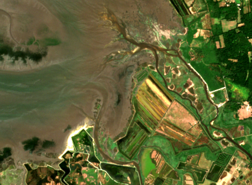
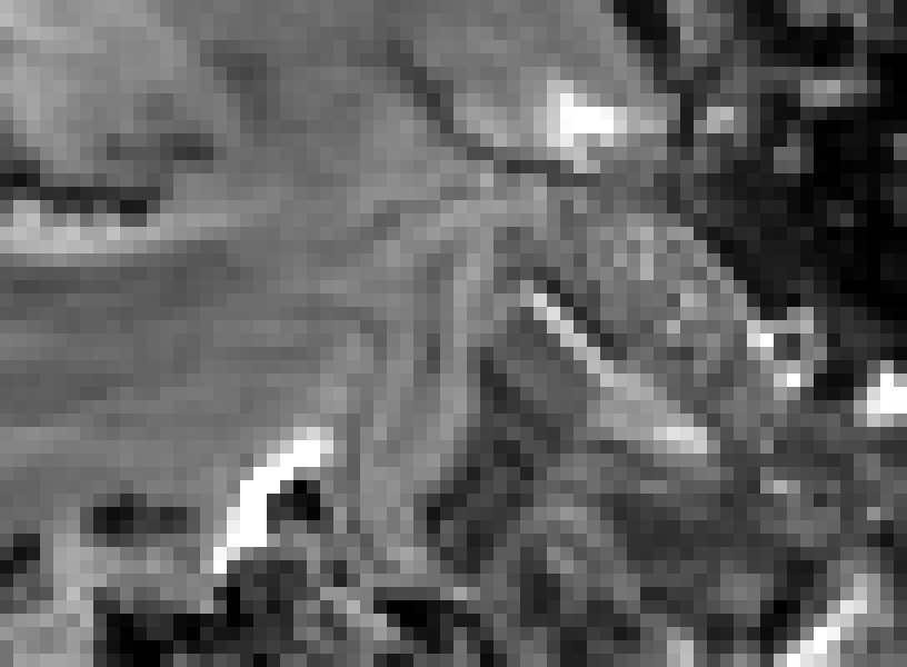
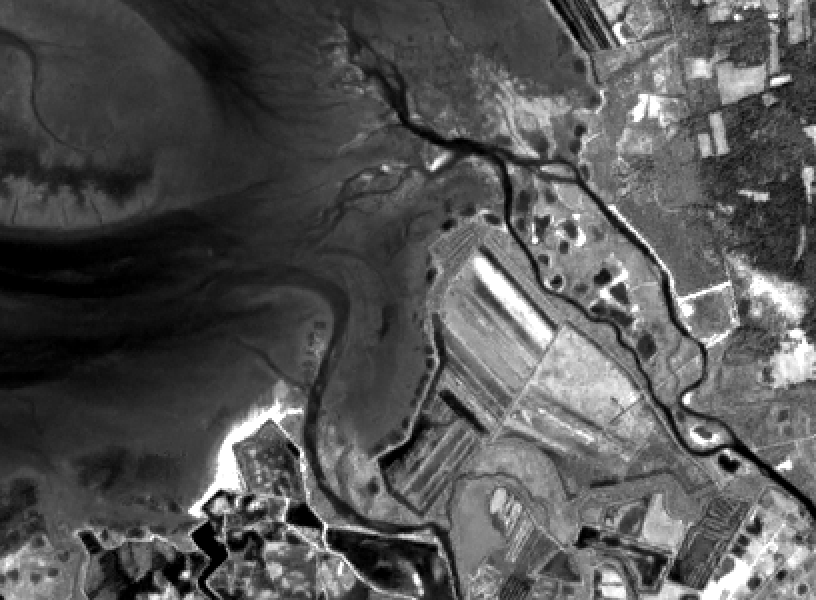
Figure 5: Top-Left: Composite image of the coastal area (delta of the Leyre river). Top-Right: Original infrared band 8 (842 nm, 10m/pixel). Middle-Left: Original band 1 (violet, 443nm, 60m/pixel). Middle-Left: Super-resolved band 1 at 10m/pixel. Bottom-left: Original band 5 (red-edge, 705nm, 20m/pixel). Bottom-right: Super-resolved band 5 at 10m/pixel.

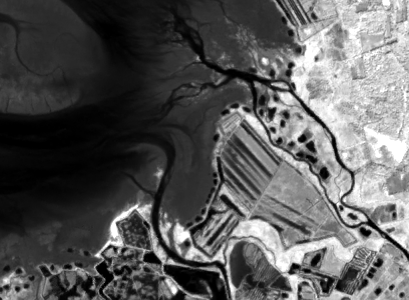
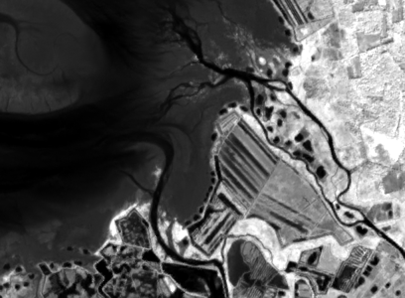
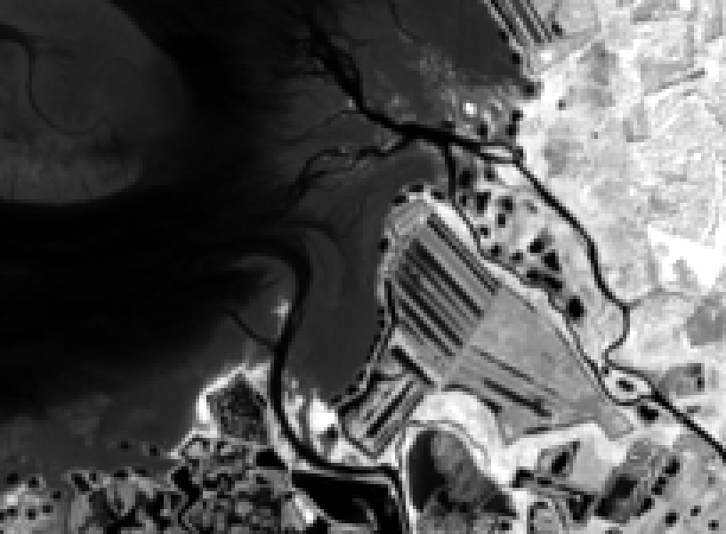
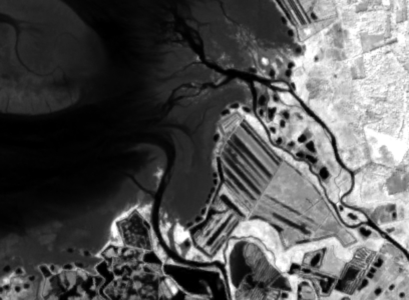
Figure 6: Coastal area (delta of the Leyre river). Top-left: Original band 6 (close infrared, 740nm, 20m/pixel). Top-right: Super-resolved band 6 at 10m/pixel. Middle-Left: Original band 7 (close infrared, 783nm, 20m/pixel). Middle-Left: Super-resolved band 7 at 10m/pixel. Bottom-left: Original band 8A (close infrared, 865nm, 20m/pixel). Bottom-right: Super-resolved band 8A at 10m/pixel.

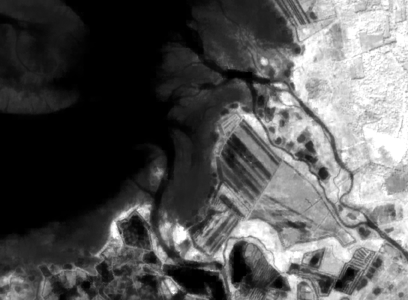
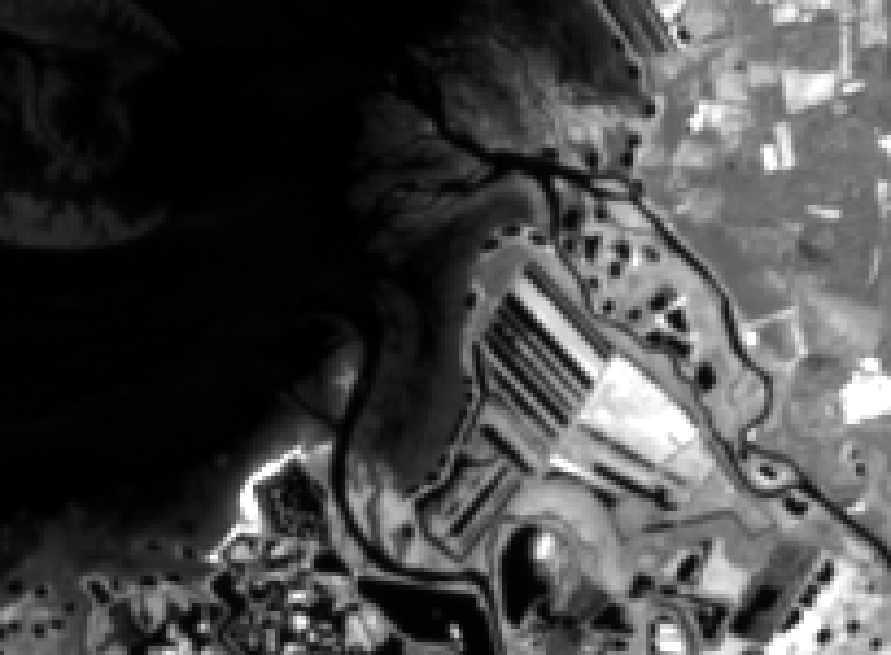
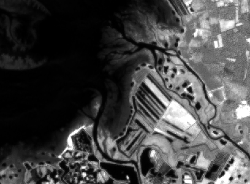
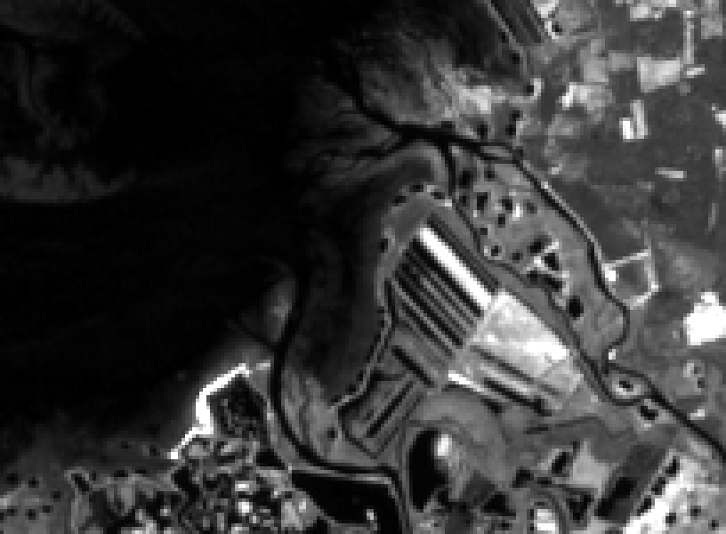
Figure 7: Coastal area (delta of the Leyre river). Top-left: Original band 9 (infrared, 945nm, 60m/pixel). Top-right: Super-resolved band 9 at 10m/pixel. Middle-Left: Original band 11 (deep infrared, 1610nm, 20m/pixel). Middle-Left: Super-resolved band 11 at 10m/pixel. Bottom-left: Original band 12 (deep infrared, 2190nm, 20m/pixel). Bottom-right: Super-resolved band 12 at 10m/pixel.

V-B Urban Area

Results for the urban environment are displayed in Figs. 8,9,10. Quantitative indicators for the 40m->20m super-resolution are :

Band	Q	ERGAS	SAM
B5 (705nm)	0.942	4.98	5.47
B6 (740nm)	0.948	3.94	4.38
B7 (783nm)	0.95	4.07	4.51
B11 (1610nm)	0.924	4.29	4.8
B12 (2190nm)	0.928	5.34	5.89
B8A (865nm)	0.956	3.76	4.17
Global	0.941	4.43	4.87

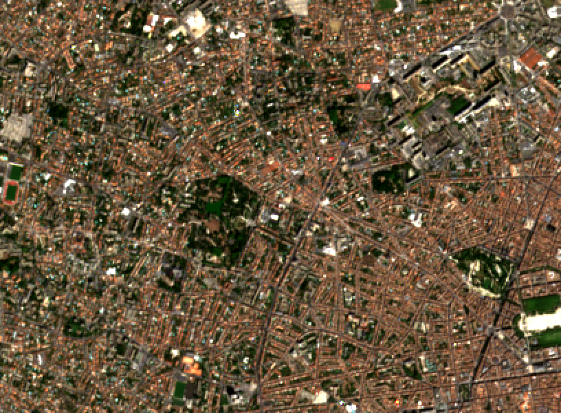
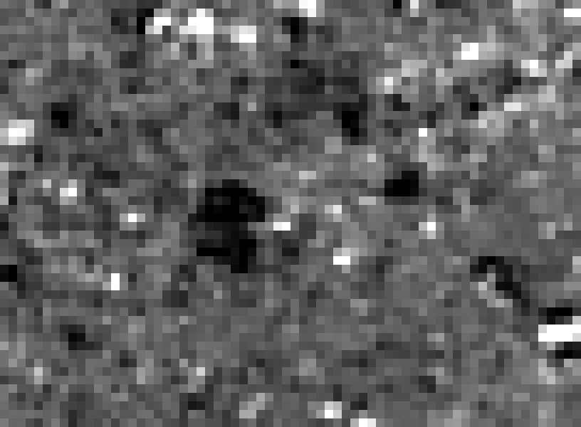
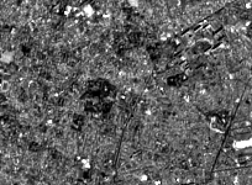
Figure 8: Top-Left: Composite image of the urban area (Bordeaux). Top-Right: Original infrared band 8 (842 nm, 10m/pixel). Middle-Left: Original band 1 (violet, 443nm, 60m/pixel). Middle-Left: Super-resolved band 1 at 10m/pixel. Bottom-left: Original band 5 (red-edge, 705nm, 20m/pixel). Bottom-right: Super-resolved band 5 at 10m/pixel.

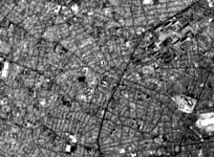
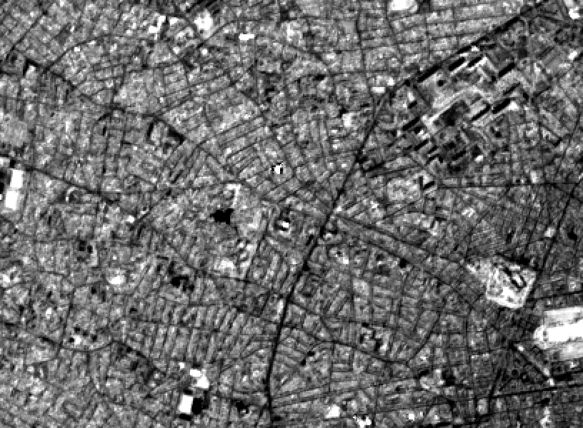
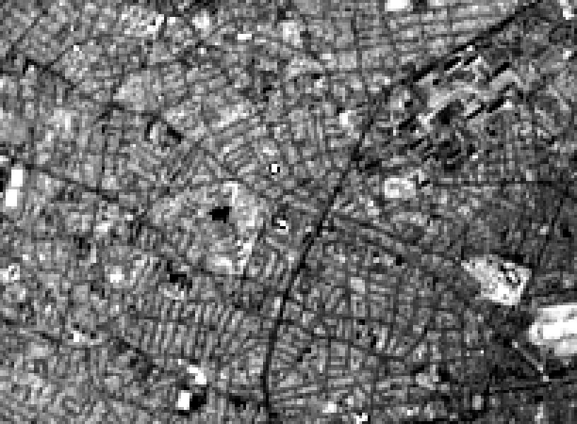
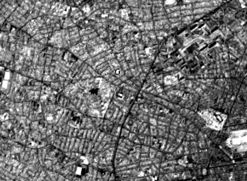
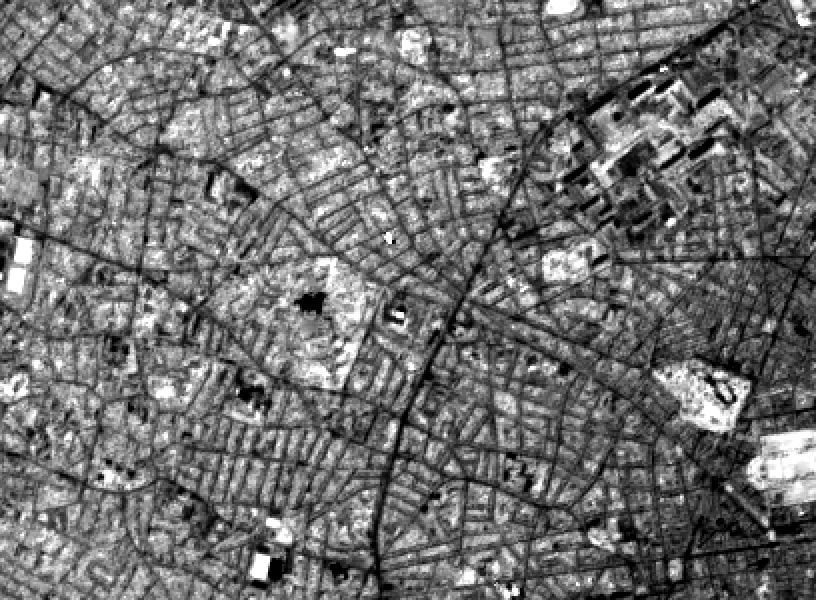
Figure 9: Urban area (Bordeaux). Top-left: Original band 6 (close infrared, 740nm, 20m/pixel). Top-right: Super-resolved band 6 at 10m/pixel. Middle-Left: Original band 7 (close infrared, 783nm, 20m/pixel). Middle-Left: Super-resolved band 7 at 10m/pixel. Bottom-left: Original band 8A (close infrared, 865nm, 20m/pixel). Bottom-right: Super-resolved band 8A at 10m/pixel.

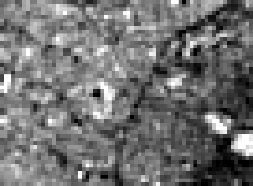
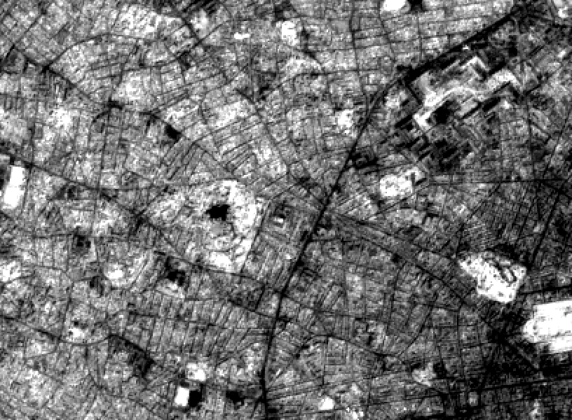
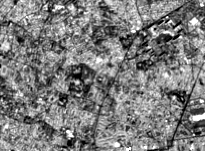
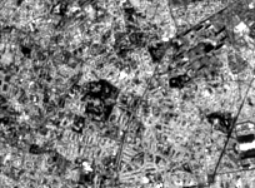
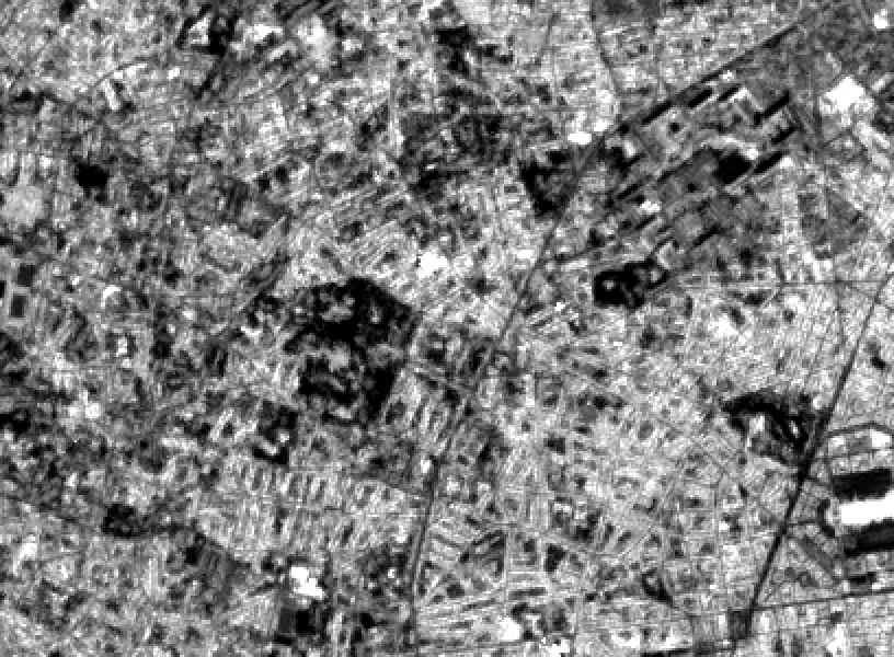
Figure 10: Urban area (Bordeaux). Top-left: Original band 9 (infrared, 945nm, 60m/pixel). Top-right: Super-resolved band 9 at 10m/pixel. Middle-Left: Original band 11 (deep infrared, 1610nm, 20m/pixel). Middle-Left: Super-resolved band 11 at 10m/pixel. Bottom-left: Original band 12 (deep infrared, 2190nm, 20m/pixel). Bottom-right: Super-resolved band 12 at 10m/pixel.

V-C Fields Area

Results for the fields environment are displayed in Figs. 11,12,13. Quantitative indicators for the 40m->20m super-resolution are :

Band	Q	ERGAS	SAM
B5 (705nm)	0.99	2.34	2.54
B6 (740nm)	0.991	1.61	1.79
B7 (783nm)	0.994	1.57	1.74
B11 (1610nm)	0.988	2.3	2.53
B12 (2190nm)	0.989	2.81	3.01
B8A (865nm)	0.994	1.47	1.63
Global	0.991	2.08	2.21

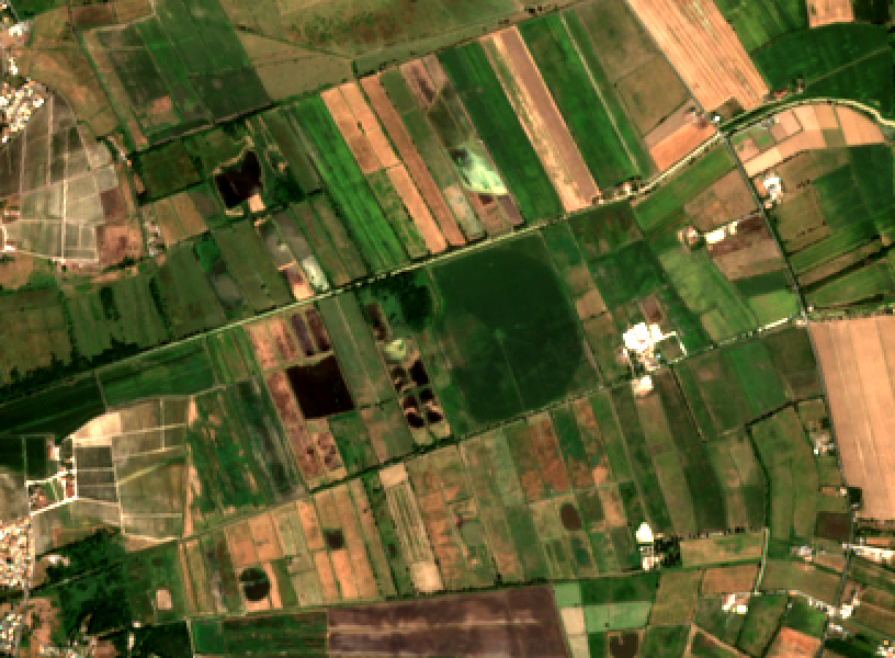
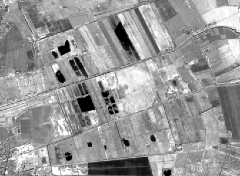
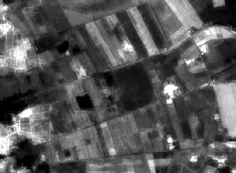
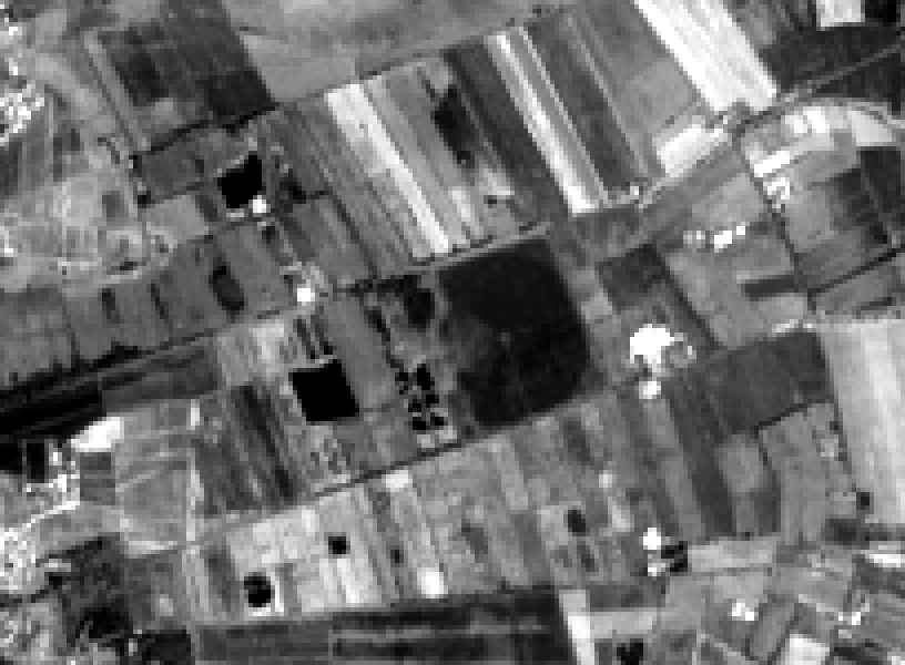
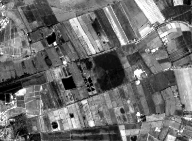
Figure 11: Top-Left: Composite image of the fields area (agriculture near bordeaux). Top-Right: Original infrared band 8 (842 nm, 10m/pixel). Middle-Left: Original band 1 (violet, 443nm, 60m/pixel). Middle-Left: Super-resolved band 1 at 10m/pixel. Bottom-left: Original band 5 (red-edge, 705nm, 20m/pixel). Bottom-right: Super-resolved band 5 at 10m/pixel.

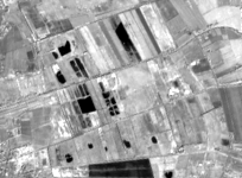
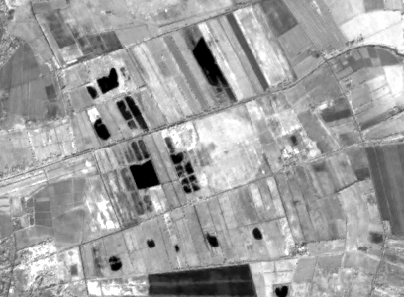
Figure 12: Fields area (agriculture near Bordeaux). Top-left: Original band 6 (close infrared, 740nm, 20m/pixel). Top-right: Super-resolved band 6 at 10m/pixel. Middle-Left: Original band 7 (close infrared, 783nm, 20m/pixel). Middle-Left: Super-resolved band 7 at 10m/pixel. Bottom-left: Original band 8A (close infrared, 865nm, 20m/pixel). Bottom-right: Super-resolved band 8A at 10m/pixel.

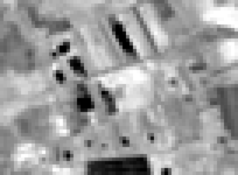
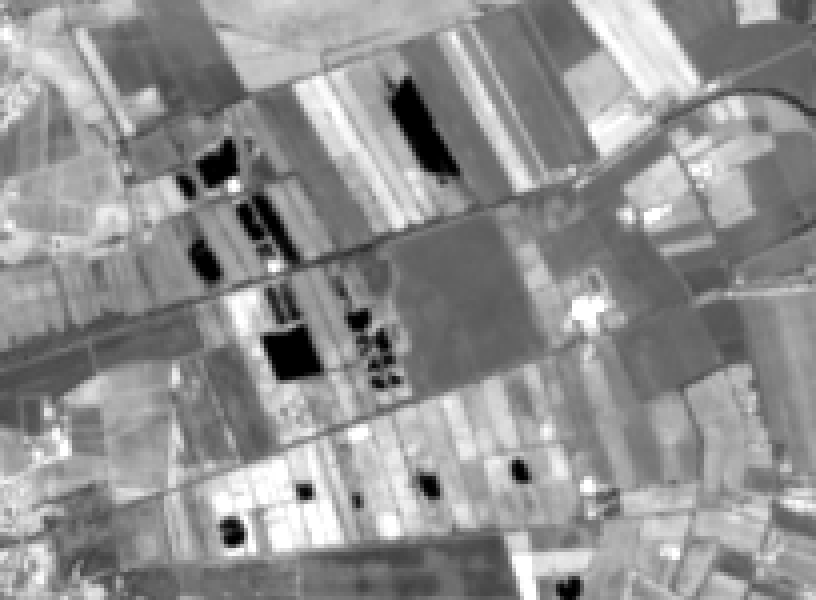
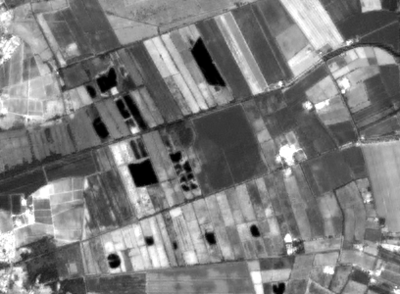
Figure 13: Fields area (agriculture near Bordeaux). Top-left: Original band 9 (infrared, 945nm, 60m/pixel). Top-right: Super-resolved band 9 at 10m/pixel. Middle-Left: Original band 11 (deep infrared, 1610nm, 20m/pixel). Middle-Left: Super-resolved band 11 at 10m/pixel. Bottom-left: Original band 12 (deep infrared, 2190nm, 20m/pixel). Bottom-right: Super-resolved band 12 at 10m/pixel.

VI Discussion

Details not present in the original bands are immediately visible in all images, especially at the largest super-resolution 60m->10m (e.g. Fig 5, middle-right). These details correspond to the band-independant information that was extracted from the other bands, and propagated to these images. Although each band presents different reflectance properties (in particular, B1 and B9), the exact same weights and geometric information extracted from Eqs. 5,6,8 were applied to all super-resolved images. This example demonstrates how the method correctly extracts band-independant information that encodes image details, while preserving the reflectance of each band (Eqs. 1,9).

Quantitative indicators are given for three typical land cover types. The method works best for agricultural environments, with large uniform areas, and worst in urban environments. Even then, Fig. 10, right, shows details that are very well recovered. Comparison with quantitative indicators from other works using panchromatic sharpening should be taken with caution. We estimate only the 40m->20m super-resolution proxy for reasons mentionned in Section IV. Nevertheless, compared to the litterature [22, 23, 6], our global averages of $0.941\leq Q\leq 0.994$, $2.08\leq ERGAS\leq 4.49$ and $2.21\leq SAM\leq 4.87$ in the different regions of interest for Sentinel-2 data are consistent with the state of art for panchromatic sharpening, albeit without a panchromatic band.

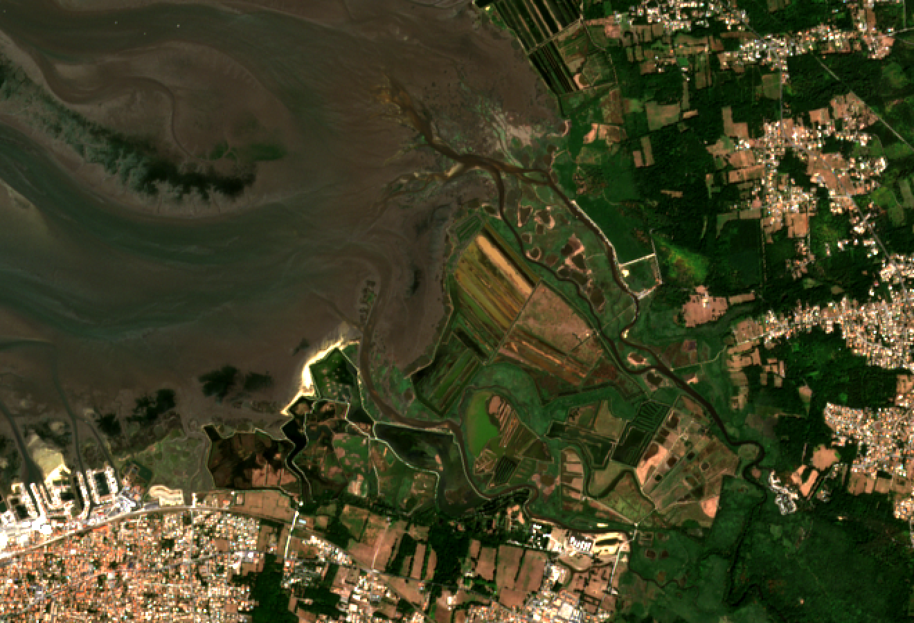
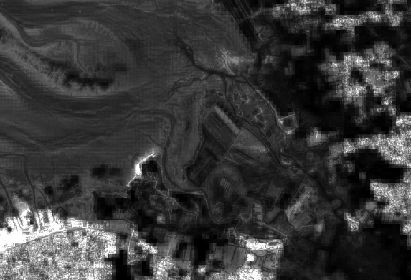
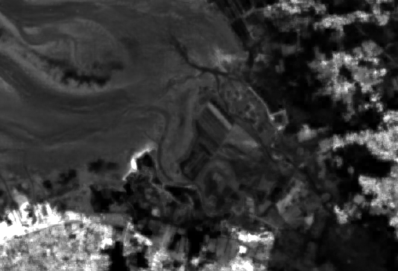
Figure 14: Top-left: RGB composite image of the enlarged coastal area, including fields and cities. Top-right: Incorrect image obtained when shared values are not used, that demonstrates their role in maintaining spatial consistency. Bottom-left: Incorrect image obtained when only mean square optimisation is applied, that shows the importance of the $\bar{q}$ ratio sharpening step described in Section III-B. Bottom-right: Incorrect image obtained when the estimation of weights $W$ is omitted while maintaning the $\bar{q}$ ratio sharpening step.

The method presented here includes multiple steps that are not trivial, but they are all necessary. In order to demonstrate this, a final experiment is performed on the coastal area, enlarged to encompass nearby cities and fields (Fig. 14). The 60m band 1 is used in order to best visualize the effect of each step. A fist idea would be to apply ratio sharpening (Eq. 8) directly on data values, instead of spatially shared values, so as to simulate panchromatic sharpening. This would simplify the method drastically. The result of this experiment is shown in Fig. 14, top-right, to be compared with the correct super-resolved result in Fig. 5, middle-right. The role of spatial consistenty is immediately highlighted: without the shared values trick, unacceptable pixel blocks are clearly visible in the result image. Conversely, why is $\bar{q}$ ratio sharpening useful? Fig. 14, bottom-left shows that it is in fact quite important for recovering the fine structures. Given that importance, one may then question the usefulness of extracting weights $W$ as band-independant information, especially since we also compute reverse weights $V$ in a second step. Why would these $W$ encode image details? Fig. 14, bottom-right shows the result of simply setting these weights to $\frac{1}{4}$ and $S^{opt}$ to the average values, as described in Section III-A, while maintaining $\bar{q}$ ratio sharpening. As expected, details are also smoothed out. Weights $W$ are defined between high-resolution pixels, hence encode high-resolution details. The reverse weights $V$ encode larger range patterns present in surrounding low-resolution pixels. Results presented in this section use the 60m/pixel band 1, for which two super-resolution steps are applied. This choice was made so as to enhance and clearly highlight the influence of shared values $S$, of $\bar{q}$ ratio sharpening, and of weights $W$, $V$, on the final result. For 20m/pixel bands only one super-resolution step is applied, but all parts of the method are still needed for good results.

Conclusion

This article presents a super-resolution method based on exploiting both the local consistency between neighborhood pixels and the geometric consistency of sub-pixel constituents across multispectral bands. Figs. 5-13 show the result of applying this method to Sentinel-2 images, in order to bring all bands from 20m/pixel and 60m/pixel down to the highest resolution at 10m/pixel. The algorithm is however generic and could be applied to other multi-resolution and multispectral satellite images. Further work could include the usage of secondary images, taken from a satellite with low temporal resolution but with a higher spatial resolution, in order to extract the geometric information used for the super-resolution. Assuming the pixel geometry does not change much between these acquisitions, then Sentinel-2 images could be enhanced below 10m/pixel. This form of multi-satellite temporal super-resolution would combine high temporal frequency with high spatial resolution. Another trail of research would be to incorporate the super-resolution algorithm directly within the atmospheric correction step [24], rather than applying it as a separate stage. Indeed, using higher-resolution pixels instead of low-resolution bands for calibrating the atmospheric correction may lead to better accuracy.

Source code

The source code for this super-resolution algorithm is provided as Free/Libre software, under either (your choice) the lesser GNU public licence v2.1 or more recent, or the CeCILL-C licence. The library is written and usable directly in C++ and it is also wrapped in a Python package. A ready to use Python script for super-resolving Sentinel-2 images is provided. See http://nicolas.brodu.net/recherche/superres/.

Appendix : Sentinel 2 bands

ESA’s Sentinel-2 program comprises two satellites (2A and 2B) with identical characteristics:

Band	Central wavelength	Bandwidth	Pixel size
B2	490 nm	65 nm	10 m
B3	560 nm	35 nm	10 m
B4	665 nm	30 nm	10 m
B8	842 nm	115 nm	10 m
B5	705 nm	15 nm	20 m
B6	740 nm	15 nm	20 m
B7	783 nm	20 nm	20 m
B8A	865 nm	20 nm	20 m
B11	1610 nm	90 nm	20 m
B12	2190 nm	180 nm	20 m
B1	443 nm	20 nm	60 m
B9	945 nm	20 nm	60 m
B10	1375 nm	30 nm	60 m

Band 10 is dedicated for cloud detection and removed by the bottom-of-atmosphere correction utility [24]. The algorithm presented in this paper nevertheless takes it into account when applied to the unprecessed, top-of-atmosphere images.

References

- [1] Julien Radoux, Guillaume Chomé, Damien Christophe Jacques, François Waldner, Nicolas Bellemans, Nicolas Matton, Céline Lamarche, Raphaël d’Andrimont and Pierre Defourny, “Sentinel-2’s Potential for Sub-Pixel Landscape Feature Detection”. Remote Sensing 8(6), p488-215, 2016.
- [2] Konstantinos G. Nikolakopoulos, “Comparison of Nine Fusion Techniques for Very High Resolution Data”. Photogrammetric Engineering & Remote Sensing 74(5), p647–659, 2008.
- [3] Allan R. Gillespie, Anne B. Kahle, Richard E. Walker, “Color enhancement of highly correlated images-II: Channel ratio and ’chromaticity’ transformation techniques”. Remote Sensing of Environment 22, p343–365, 1987.
- [4] Chris Padwick, Michael Deskevich, Fabio Pacifici, Scott Smallwood, “WorldView-2 pan-sharpening”. Proceedings of the ASPRS 2010 Annual Conference Vol. 2630, 2010.
- [5] Pat S. Chavez, Stuart C. Sides, Jeffrey A. Anderson, “Comparison of three different methods to merge multiresolution and multispectral data: landsat TM and SPOT panchromatic”. Photogrammetric Engineering and Remote Sensing 57(3), p295-303, 1991.
- [6] Bo Wu, Qiankun Fu,Liya Sun, Xiaoqin Wang, “Enhanced hyperspherical color space fusion technique preserving spectral and spatial content”, Journal of Applied Remote Sensing 9, p097291-1/18, 2015.
- [7] Yu He, Kim-Hui Yap, Li Chen, Lap-Pui Chau, “A soft MAP framework for blind super-resolution image reconstruction”. Image and Vision Computing 27, p364-373, 2009.
- [8] Rafael Molina, Miguel Vega, Javier Mateos, Aggelos K. Katsaggelos, “Variational posterior distribution approximation in Bayesian super resolution reconstruction of multispectral images”. Applied and Computational Harmonic Analysis 24(2), p251-267, 2008.
- [9] Shinji Nakazawa and Akira Iwasaki, “Super-resolution imaging using remote sensing platform”. Proceedings of the IEEE Geoscience and Remote Sensing Symposium, pp. 1987-1990, 2014.
- [10] Simon Baker, Takeo Kanade, “Limits on super-resolution and how to break them”. IEEE Transactions on Pattern Analysis and Machine Intelligence 24(9), p1167-1183, 2002.
- [11] Lukas Liebel, Marco Körner, “Single-Image super resolution for multispectral remote sensing data using convolutional neural networks”. XXIII ISPRS Congress proceedings p883-890, 2016.
- [12] William T. Freeman, Thouis R. Jones, Egon C. Pasztor, “Example-based super-resolution”. IEEE Computer Graphics and Applications 22(2), p56-65, 2002.
- [13] Kwang In Kim, Younghee Kwon, “Example-based learning for single-image super-resolution”. Joint Pattern Recognition Symposium proceedings p456-465, 2008.
- [14] Chao Dong, Chen Change Loy, Kaiming He, Xiaoou Tang, “Image super-resolution using deep convolutional networks”. IEEE transactions on pattern analysis and machine intelligence 38(2), p295-307, 2016.
- [15] Connelly Barnes, Eli Shechtman, Adam Finkelstein, Dan B. Goldman, “PatchMatch: a randomized correspondence algorithm for structural image editing”. ACM Transactions on Graphics-TOG 28(3), p24-33, 2009.
- [16] Feng Li, Xiuping Jia, Donald Fraser, “Superresolution Reconstruction of Multispectral Data for Improved Image Classification”. IEEE Geoscience and Remote Sensing Letters 6(4), p689-693, 2009.
- [17] Teerasit Kasetkasema, Manoj K. Arora, Pramod K. Varshney, “Super-resolution land cover mapping usingfield based approach a Markov random”. Remote Sensing of Environment 96, p302-314, 2005.
- [18] Antonio Turiel, Hussein Yahia, Conrad Pérez-Vicente, “Microcanonical multifractal formalism—a geometrical approach to multifractal systems: Part I. Singularity analysis”. Journal of Physics A: Mathematical and Theoretical 41, p015501-015536, 2008.
- [19] Joël Sudre, Hussein Yahia, Oriol Pont, Véronique Garçon, “Ocean Turbulent Dynamics at Superresolution From Optimal Multiresolution Analysis and Multiplicative Cascade”. IEEE Transactions on Geoscience and Remote Sensing 53(11), p6274-6285, 2015.
- [20] J.J.Settle and N.A. Drake, “Linear mixing and the estimation of ground cover proportions”. International Journal of Remote Sensing 14(6), p1159-1177, 1993.
- [21] Sameer Agarwal and Keir Mierle and Others, “Ceres Solver”. Available online: http://ceres-solver.org (accessed on 20 September 2016).
- [22] Lucien Wald, “Quality of high resolution synthesised images: Is there a simple criterion ?”. Third conference ”Fusion of Earth data: merging point measurements, raster maps and remotely sensed images”, Sophia Antipolis, France, Jan 2000, SEE/URISCA, pp.99-103, 2000, hal-00395027.
- [23] Luciano Alparone, Bruno Aiazzi, Stefano Baronti, Andrea Garzelli, Filippo Nencini, and Massimo Selva, “Multispectral and Panchromatic Data Fusion Assessment Without Reference”. Photogrammetric Engineering & Remote Sensing 74(2), p193-200, 2008.
- [24] Sentinel-2 MSI – Level-2A version 2.2.1, may 2016. Available online: http://step.esa.int/main/third-party-plugins-2/sen2cor/ (accessed on 19 September 2016).