Algebraic Tools for the Analysis of State Space Models

Abstract.

We present algebraic techniques to analyze state space models in the areas of structural identifiability, observability, and indistinguishability. While the emphasis is on surveying existing algebraic tools for studying ODE systems, we also present a variety of new results. In particular: On structural identifiability, we present a method using linear algebra to find identifiable functions of the parameters of a model for unidentifiable models. On observability, we present techniques using Gröbner bases and algebraic matroids to test algebraic observability of state space models. On indistinguishability, we present a sufficient condition for distinguishability using computational algebra and demonstrate testing indistinguishability.

1. Introduction

Consider a dynamic systems model in the following state space form:

(1) $$x^{\prime}(t)=f(x(t),p,u(t))\quad\quad\quad y(t)=g(x(t),p)$$

Here $x(t)$ is the state variable vector, $u(t)$ is the input vector (or control vector), $y(t)$ is the output vector, and $p$ is a parameter vector $(p_{1},...,p_{n})$ composed of unknown real parameters $p_{1},...,p_{n}$. In this modeling framework the only observed quantities are the input and output trajectories, $u(t)$ and $y(t)$ (or more realistically, the trajectories observed at some finite number of time points $t_{1},t_{2},\ldots$), together with the underlying modeling structure (that is, the functions $f$ and $g$). State space models are widely used throughout the applied sciences, including the areas of control [27, 52, 58, 67], systems biology [22], economics and finance [34, 76], and probability and statistics [11, 39].

A simple example of a state space model is a linear compartment model.

Example 1.1.

Consider the following ODE:

$$\begin{pmatrix}x_{1}^{\prime}\\ x_{2}^{\prime}\end{pmatrix}={\begin{pmatrix}-(a_{01}+a_{21})&a_{12}\\ a_{21}&-(a_{02}+a_{12})\end{pmatrix}}{\begin{pmatrix}x_{1}\\ x_{2}\end{pmatrix}}+{\begin{pmatrix}u_{1}\\ 0\end{pmatrix}}\quad\quad y_{1}=x_{1}.$$

This model is called the linear 2-compartment model and will be referenced in later sections. Here $(x_{1}(t),x_{2}(t))$ is the state variable vector, $u_{1}(t)$ is the input (or control), $y_{1}(t)$ is the output, and $(a_{01},a_{02},a_{12},a_{21})$ is the unknown parameter vector.

Although the analysis of the behavior and use of state space models falls under the dynamical systems research area umbrella, tools from algebra can be used to analyze these models when the functions $f$ and $g$ are rational functions. Algebraic methods typically focus on determining which key features that the models satisfy a priori before the models are used to analyze data. The point of the present paper is to give an overview of these algebraic techniques to show how they can be applied to analyze state space models. We focus on three main problems where algebraic techniques can be helpful: determining structural identifiability, observability, and indistinguishability of the models. We provide an overview of techniques for these problems coming from computational algebra and we also introduce some new results coming from matroid theory.

2. State Space Models

In this section, we provide a more detailed introduction to state space models, and the basic theoretical problems of identifiability, observability, and indistinguishability that we will address in this paper. We also provide a detailed introduction to the linear compartment models that will be an important set of examples that we use to illustrate the theory.

Consider a general state space model

(2) $$x^{\prime}(t)=f(x(t),p,u(t))\quad\quad\quad y(t)=g(x(t),p)$$

as in the introduction, with $x(t)\in\mathbb{R}^{N}$, $y(t)\in\mathbb{R}^{M}$, $u(t)\in\mathbb{R}^{R}$ and $p\in\mathbb{R}^{n}$.

The state space model (2) is called identifiable if the unknown parameter vector $p$ can be recovered from observation of the input and output alone. The model is observable if the trajectories of the state space variables $x(t)$ can be recovered from observation of the input and output alone. Two state space models are indistinguishable if for any choice of parameters in the first model, there is a choice of parameters in the second model that will yield the same dynamics in both models, and vice versa. Before getting into the technical details of these definitions for state space models, we introduce some key examples of state space models that we will use to illustrate the main concepts throughout the paper.

Example 2.1 (SIR Model).

A commonly used model in epidemiology is the Susceptible-Infected-Recovered model (SIR model) ([8],[9],[10],[46],[62]) which has the following form:

$$S^{\prime} =\mu N-\beta SI-\mu S$$

$$I^{\prime} =\beta SI-(\mu+\gamma)I$$

$$R^{\prime} =\gamma I-\mu R$$

$$y =kI$$

The interpretation of the state variables is that $S(t)$ is the number of susceptible individuals at time $t$, $I(t)$ is the number of infected individuals at time $t$, and $R(t)$ is the number of recovered individuals at time $t$. The unknown parameters are the birth/death rate $\mu$, the transmission parameter $\beta$, the recovery rate $\gamma$, the total population $N$, and the proportion of the infected population measured $k$. In this model, we assume that we only observe the trajectory $y(t)$, an (unknown) proportion of the infected population. Note that this simple model has no input/control.

Identifiability and observability analysis in this model are concerned with determining which unmeasured quantities can be determined from only the observed output trajectory $y$. Identifiability specifically concerns the unobserved parameters $\mu,\beta,\gamma,N$, and $k$, whereas observability specifically is concerned with the unobserved state variables $S$, $I$, and $R$. ∎

A commonly used family of state space models are the linear compartment models. We outline these models here. Let $G=(V,E)$ be a directed graph with vertex set $V$ and set of directed edges $E$. Each vertex $i\in V$ corresponds to a compartment in our model and each edge $j\rightarrow i$ corresponds to a direct flow of material from the $j$th compartment to the $i$th compartment. Let $In,Out,Leak\subseteq V$ be three sets of compartments: the set of input compartments, output compartments, and leak compartments respectively. To each edge $j\rightarrow i$ we associate an independent parameter $a_{ij}$, the rate of flow from compartment $j$ to compartment $i$. To each leak node $i\in Leak$, we associate an independent parameter $a_{0i}$, the rate of flow from compartment $i$ leaving the system.

To such a graph $G$ and set of leaks $Leak$ we associate the matrix $A(G)$ in the following way:

$$A(G)_{ij}=\left\{\begin{array}[]{l l l}-a_{0i}-\sum_{k:i\rightarrow k\in E}{a_{ki}}&\quad\text{if $i=j$ and }i\in Leak\\ -\sum_{k:i\rightarrow k\in E}{a_{ki}}&\quad\text{if $i=j$ and }i\notin Leak\\ a_{ij}&\quad\text{if $j\rightarrow{i}$ is an edge of $G$}\\ 0&\quad\text{otherwise}\\ \end{array}\right.$$

For brevity, we will often use $A$ to denote $A(G)$. Then we construct a system of linear ODEs with inputs and outputs associated to the quadruple $(G,In,Out,Leak)$ as follows:

(3) $$x^{\prime}(t)=Ax(t)+u(t)\quad\quad y_{i}(t)=x_{i}(t)\mbox{ for }i\in Out$$

where $u_{i}(t)\equiv 0$ for $i\notin In$. The coordinate functions $x_{i}(t)$ are the state variables, the functions $y_{i}(t)$ are the output variables, and the nonzero functions $u_{i}(t)$ are the inputs. The resulting model is called a linear compartment model.

We use the following convention for drawing linear compartment models [22]. Numbered vertices represent compartments, outgoing arrows from the compartments represent leaks, an edge with a circle coming out of a compartment represents an output, and an arrowhead pointing into a compartment represents an input.

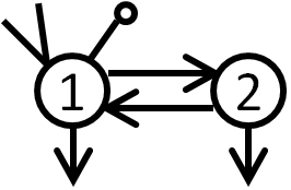
Figure 1. A 2-compartment model with $In=\{1\}$, $Out=\{1\}$, and $Leak=\{1,2\}$.

Example 2.2.

For the compartment model in Figure 1, the ODE system has the form given in Example 1.1. Since this model has a leak in every compartment, the diagonal entries of $A(G)$ are algebraically independent of the other entries. In this situation, we can re-write the diagonal entries of the matrix $A$ as $a_{11}=-(a_{01}+a_{21})$ and $a_{22}=-(a_{02}+a_{12})$. Thus we have the following ODE system:

$$\begin{pmatrix}x_{1}^{\prime}\\ x_{2}^{\prime}\end{pmatrix}={\begin{pmatrix}a_{11}&a_{12}\\ a_{21}&a_{22}\end{pmatrix}}{\begin{pmatrix}x_{1}\\ x_{2}\end{pmatrix}}+{\begin{pmatrix}u_{1}\\ 0\end{pmatrix}}\quad\quad y_{1}=x_{1}.$$

3. Differential Algebra Approach To Identifiability

In this paper we focus on the structural versions of identifiability, observability, and indistinguishability (that is, structural identifiability, structural observability, structural indistinguishability). That means we study when these properties hold assuming that we are able to observe trajectories perfectly. Practical versions of these problems concern how noise affects the ability to, e.g., infer parameters of the models. Structural answers are important because the structural version of the condition is necessary to insure that the practical version holds. On the other hand, practical versions of these problems depend on the specific data dependent context in which the data might be observed, and might further depend on the particular underlying unknown parameter choices. We will drop “structural” throughout the paper since this will be implicit in the majority of our discussion.

To make the definitions of identifiability, observability, and indistinguishability precise we will use tools from differential algebra. In this approach, we must form the input-output equations associated to our model by performing differential elimination. We carry out operations in the differential ring

$$\mathbb{Q}(p)[x,y,u,x^{\prime},y^{\prime},u^{\prime},\ldots]$$

with the derivation $\frac{d}{dt}$ with respect to time such that the parameters $p$ are constants with respect to the derivation, and $\frac{d}{dt}x=x^{\prime}$, etc. Differential algebra was developed by Ritt [59] and Kolchin [40] and has its most well-known applications to the study of the algebraic solution to systems of differential equations [63].

The goal of this differential elimination process for state space models is to eliminate the state variables $x(t)$ and their derivatives, so that the resulting equations are purely in terms of the input variables, output variables, and the parameters. The equations that result from applying the differential elimination process are called the input-output equations. We obtain input-output equations in the following form:

$$\sum_{i}{c_{i}(p)\psi_{i}(u,y)=0}$$

where $c_{i}(p)$ are rational functions in the parameter vector $p$ and $\psi_{i}(u,y)$ are differential monomials in $u(t)$ and $y(t)$. Let $c=(c_{1}(p),...,c_{m}(p))$ denote the vector of coefficients of the input-output equations, which are rational functions in the parameter vector $p$. This coefficient vector induces a map $c:\mathbb{R}^{n}\rightarrow\mathbb{R}^{m}$ called the coefficient map, that plays an important role in the study of identifiability and indistinguishability.

For general state space models of the form (2) we can also use ordinary Gröbner basis calculations to determine the input/output equation.

Proposition 3.1.

Consider a state space model of the form (2) where $f$ and $g$ are polynomial functions and where there are $N$ state-space variables, $M=1$ output variable, and $R$ input variables. Let $P$ be the ideal

$$\langle x^{\prime}-f(x,p,u),\,\ldots,\,x^{(N)}-\frac{d^{N-1}}{dt^{N-1}}f(x,p,u),\,y-g(x,p),\,\ldots,\,y^{(N)}-\frac{d^{N}}{dt^{N}}g(x,p)\rangle\\ \subseteq\mathbb{Q}(p)[x,y,u,x^{\prime},y^{\prime},u^{\prime},\ldots,x^{(N-1)},y^{(N-1)},u^{(N-1)},x^{(N)},y^{(N)}].$$

Then $P\cap\mathbb{Q}(p)[y,u,y^{\prime},u^{\prime},\ldots,y^{(N-1)},u^{(N-1)},y^{(N)}]$ is not the zero ideal and hence contains an input-output equation.

Although Proposition 3.1 is known in the literature [28, 36], we include a proof because it will illustrate some useful ideas that we will use in other new results later on. Note that although this is stated for a single output, one can apply Proposition 3.1 one output at a time to find input/output equations for each output separately and hence obtain Proposition 3.2.

Proof.

Note that $P$ is a prime ideal, since, with a carefully chosen lexicographic term order, it has as its initial ideal

$$\langle x^{\prime},\ldots,x^{(N)},y,\ldots,y^{(N)}\rangle$$

which is a prime ideal. Since $P$ is prime, we can consider the algebraic matroid associated to this ideal. To say that $P\cap\mathbb{Q}(p)[y,u,y^{\prime},u^{\prime},\ldots,y^{(N-1)},u^{(N-1)},y^{(N)}]$ is not the zero ideal is equivalent to saying that the set $\{y,u,y^{\prime},u^{\prime},\ldots,y^{(N-1)},u^{(N-1)},y^{(N)}\}$ is a dependent set in the associated algebraic matroid. The initial ideal also shows that this ideal is a complete intersection, so it is has codimension $N^{2}+N+1$ (since this is the number of equations involved). The total number of variables in our polynomial ring is $N(N+1)+N+1+RN$, where $N(N+1)$ counts the $x,x^{\prime},\ldots$ variables, $N+1$ counts the $y,y^{\prime},\ldots$ variables, and $RN$ counts the $u,u^{\prime},\ldots$ variables. Thus $P$ has dimension $N+RN$. Since the total number of variables in the set $\{y,u,y^{\prime},u^{\prime},\ldots,y^{(N-1)},u^{(N-1)},y^{(N)}\}$ is $N+1+RN$, these variables must be dependent, i.e. there must exist a relation. ∎

For multiple outputs, one can again take derivatives up to order $N$ and show that there must exist an input-output equation for each output:

Proposition 3.2.

Consider a state space model of the form (2) where $f$ and $g$ are polynomial functions and where there are $N$ state-space variables, $M$ output variables, and $R$ input variables. Let $P$ be the ideal

$$\langle x^{\prime}-f(x,p,u),\,\ldots,\,x^{(N)}-\frac{d^{N-1}}{dt^{N-1}}f(x,p,u),\,y-g(x,p),\,\ldots,\,y^{(N)}-\frac{d^{N}}{dt^{N}}g(x,p)\rangle\\ \subseteq\mathbb{Q}(p)[x,y,u,x^{\prime},y^{\prime},u^{\prime},\ldots,x^{(N-1)},y^{(N-1)},u^{(N-1)},x^{(N)},y^{(N)}].$$

Then $P\cap\mathbb{Q}(p)[y_{i},u,y_{i}^{\prime},u^{\prime},\ldots,y_{i}^{(N-1)},u^{(N-1)},y_{i}^{(N)}]$ is not the zero ideal and hence contains an input-output equation for each $y_{i}$.

Proof.

We follow the proof of Proposition 3.1. The number of equations involved is $N^{2}+M(N+1)$. The total number of variables in our polynomial ring is $N(N+1)+M(N+1)+RN$. Here $N(N+1)$ counts the $x,x^{\prime},\ldots$ variables, $M(N+1)$ counts the $y,y^{\prime},\ldots$ variables, and $RN$ counts the $u,u^{\prime},\ldots$ variables. Thus $P$ has dimension $N+RN$. For each $y_{i}$, the total number of variables in the set $\{y_{i},u,y_{i}^{\prime},u^{\prime},\ldots,y_{i}^{(N-1)},u^{(N-1)},y_{i}^{(N)}\}$ is $N+1+RN$. Thus these variables must be dependent, i.e. there must exist a relation for each $y_{i}$. ∎

Note that one could also work with smaller ideals than $P$ with only up to $k\leq N$ derivatives, as in [47]. In some instances this might produce an input output equation, but the dimension guarantee that ensures the existence of an input/output equation only occurs when $k=N$.

Example 3.3.

Consider the SIR model from Example 2.1. The ideal $P$ in this example is:

$$\langle S^{\prime}-\mu S-bSI+\mu N,\,S^{\prime\prime}-\mu S^{\prime}-\beta SI^{\prime}-\beta S^{\prime}I,\,S^{\prime\prime\prime}-\mu S^{\prime\prime}-\beta SI^{\prime\prime}-2\beta S^{\prime}I^{\prime}-\beta S^{\prime\prime}I,\,\\ I^{\prime}-(\mu+\gamma)I+\beta SI,\,I^{\prime\prime}-(\mu+\gamma)I^{\prime}+\beta S^{\prime}I-\beta SI^{\prime},\,I^{\prime\prime\prime}-(\mu+\gamma)I^{\prime\prime}+\beta S^{\prime\prime}I-2\beta S^{\prime}I^{\prime}-\beta SI^{\prime\prime},\,\\ R^{\prime}-\mu R+\gamma I,\,R^{\prime\prime}-\mu R^{\prime}+\gamma I^{\prime},\,R^{\prime\prime\prime}-\mu R^{\prime\prime}+\gamma I^{\prime\prime},\,\\ y-kI,\,y^{\prime}-kI^{\prime},\,y^{\prime\prime}-kI^{\prime\prime},\,y^{\prime\prime\prime}-kI^{\prime\prime\prime}\rangle.$$

This model has no input, so in this case we get a single output equation in the output variable $y$ and the parameters $\mu,\beta,\gamma,N,$ and $k$. The output equation is:

$$(-\beta kN\mu+kN\mu^{2}+kN\mu\gamma)y^{2}+(\beta\mu+\beta\gamma)y^{3}+kN\mu yy^{\prime}+\beta y^{2}y^{\prime}-kNy^{\prime 2}+kNyy^{\prime\prime}=0.$$

This differential equation has $6$ differential monomials $y^{2},y^{3},yy^{\prime},y^{2}y^{\prime},y^{\prime 2},yy^{\prime\prime},$ so the coefficient vector $c$ gives a function from $\mathbb{R}^{5}$ to $\mathbb{R}^{6}$, given by

$$c:\mathbb{R}^{5}\rightarrow\mathbb{R}^{6},\quad(\mu,\beta,\gamma,N,k)\mapsto(-\beta kN\mu+kN\mu^{2}+kN\mu\gamma,\beta\mu+\beta\gamma,kN\mu,\beta,-kN,kN).$$

The dynamics of the input and output will only depend on the input-output equation up to a nonzero constant multiple. Hence, the coefficient map is only truly well-defined up to scalar multiplication. There are two natural ways to deal with this issue. The most appealing for an algebraist is to treat the coefficient map as a map into projective space: $c:\mathbb{R}^{n}\rightarrow\mathbb{R}\mathbb{P}^{m-1}$. The second approach is to force the equation to have a fixed form that will avoid this issue, by forcing the equation to be monic by dividing through by one of the coefficients. We will take the second approach in this paper. In the output equation in Example 3.3, one possible normalization yields the coefficient map

$$c:\mathbb{R}^{5}\rightarrow\mathbb{R}^{6},\quad(\mu,\beta,\gamma,N,k)\mapsto(-\beta\mu+\mu^{2}+\mu\gamma,\frac{\beta\mu+\beta\gamma}{kN},\mu,\frac{\beta}{kN},-1,1).$$

In the standard differential algebra approach to identifiability, we assume that the coefficients $c_{i}(p)$ of the input-output equations can be recovered uniquely from the input-output data, and thus are assumed to be known quantities. This is a reasonable assumption when the input $u$ is a general enough function and the parameters are generic: in this case the dynamics will yield a unique differential equation. The identifiability question is then: can the parameters of the model be recovered from the coefficients of the input-output equations?

Definition 3.4.

Let $c=(c_{1}(p),...,c_{m}(p))$ denote the vector of coefficients of the input-output equations, which are rational functions in the parameter vector $p$, which we assume to be normalized so that the input-output equations are monic. We consider $c$ as a function from some natural open biologically relevant parameter space $\Theta\subseteq\mathbb{R}^{n}$.

• The model is globally identifiable if $c:\Theta\rightarrow\mathbb{R}^{m}$ is a one-to-one function.

• The model is generically globally identifiable if there is a dense open subset $\Theta^{\prime}\subseteq\Theta$ such that $c:\Theta^{\prime}\rightarrow\mathbb{R}^{m}$ is one-to-one.

• The model is locally identifiable if around any point $p\in\Theta$ there is an open neighborhood $U_{p}\subseteq\Theta$ such that $c:U_{p}\rightarrow\mathbb{R}^{m}$ is a one-to-one function.

• The model is generically locally identifiable if there is a dense open subset $\Theta^{\prime}\subseteq\Theta$ such that for all $p\in\Theta^{\prime}$ there is an open neighborhood $U_{p}\subseteq\Theta^{\prime}$ such that $c:U_{p}\rightarrow\mathbb{R}^{m}$ is a one-to-one function.

• The model is unidentifiable if there is a $p\in\Theta$ such that $c^{-1}(c(p))$ is infinite.

• The model is generically unidentifiable if there is a dense subset $\Theta^{\prime}\subseteq\Theta$ such that for all $p\in\Theta^{\prime}$, $c^{-1}(c(p))$ is infinite.

As can be seen, there are many different variations on the notions of identifiability. Because of problems that might arise on sets of measure zero that can ruin the strongest form of global identifiability, one usually needs to add the generic conditions to get meaningful results. In this paper, we will consider state space models (2) where $f$ and $g$ are polynomial (or rational) functions. This ensures, via the differential elimination procedure, that the coefficient function $c(p)$ is a rational function of the parameters. For linear compartment models this can always be taken to be polynomial functions.

In this paper, we will also focus almost exclusively on generic local identifiability and generic nonidentifiability and will use the following result to determine which of these conditions the model satisfies.

Proposition 3.5.

The model is generically locally identifiable if and only if the rank of the Jacobian of $c$ is equal to $n$ when evaluated at a generic point. Conversely, if the rank of the Jacobian of $c$ is less than $n$ for all choices of the parameters then the model is generically unidentifiable.

Proof.

Since the coefficients in $c$ are all polynomial or rational functions of the parameters, the model is generically locally identifiable if and only if the image of $c$ has dimension equal to the number of parameters, i.e. $n$. The dimension of the image of a map is equal to the evaluation of the Jacobian at a generic point. ∎

Example 3.6.

SIR Model From Example 3.3, we have the following coefficient map:

$$c:\mathbb{R}^{5}\rightarrow\mathbb{R}^{6},\quad(\mu,\beta,\gamma,N,k)\mapsto(-\beta\mu+\mu^{2}+\mu\gamma,\frac{\beta\mu+\beta\gamma}{kN},\mu,\frac{\beta}{kN},-1,1).$$

We obtain the Jacobian with respect to the parameter ordering $(k,N,\mu,\gamma,\beta)$:

$$\begin{pmatrix}0&0&-\beta+2\mu+\gamma&\mu&\mu\\ \frac{-(\mu+\gamma)\beta}{k^{2}N}&\frac{-(\mu+\gamma)\beta}{kN^{2}}&\frac{\beta}{kN}&\frac{\beta}{kN}&\frac{(\mu+\gamma)}{kN}\\ 0&0&1&0&0\\ \frac{-\beta}{k^{2}N}&\frac{-\beta}{kN^{2}}&0&0&\frac{1}{kN}\\ 0&0&0&0&0\\ 0&0&0&0&0\end{pmatrix}.$$

Since the rank of the Jacobian at a generic point is $4$, not $n=5$, the model is generically unidentifiable.

3.1. Input-output equations for linear models

There have been several methods proposed to find the input-output equations of nonlinear ODE models [3, 5, 25, 26, 42, 47, 53], but for linear models the problem is much simpler. We use Cramer’s rule in the following theorem, whose proof can be found in [49]:

Theorem 3.7.

Let $\partial$ be the differential operator $d/dt$ and let $A_{ji}$ be the submatrix of $\partial{I}-A$ obtained by deleting the $jth$ row and the $ith$ column of $\partial{I}-A$. Then the input-output equations are of the form:

$$\frac{\det(\partial{I}-A)}{g_{i}}y_{i}=\sum_{j\in In}(-1)^{i+j}\frac{\det(A_{ji})}{g_{i}}u_{j}$$

where $g_{i}$ is the greatest common divisor of $\det(\partial{I}-A)$, $\det(A_{ji})$ such that $j\in In$ for a given $i\in Out$.

Example 3.8.

Linear Compartment Model. For the linear 2-compartment model from Example 2.2, we obtain the following input-output equation:

$$y_{1}^{\prime\prime}-(a_{11}+a_{22})y_{1}^{\prime}+(a_{11}a_{22}-a_{12}a_{21})y_{1}=u_{1}^{\prime}-a_{22}u_{1}.$$

Thus we have the following coefficient map:

$$c:\mathbb{R}^{4}\rightarrow\mathbb{R}^{5},\quad(a_{11},a_{22},a_{12},a_{21})\mapsto(1,-a_{11}-a_{22},a_{11}a_{22}-a_{12}a_{21},1,-a_{22}).$$

We obtain the Jacobian with respect to the parameter ordering $(a_{11},a_{22},a_{12},a_{21})$:

$$\begin{pmatrix}0&0&0&0\\ -1&-1&0&0\\ a_{22}&a_{11}&-a_{21}&-a_{12}\\ 0&0&0&0\\ 0&-1&0&0\end{pmatrix}.$$

Since the rank of the Jacobian at a generic point is $3$, not $n=4$, the model is generically unidentifiable.

4. Identifiable functions

One issue that arises in identifiability analysis of state space models is figuring out what to do with a model that is generically unidentifiable. In some circumstances, the natural approach is to develop a new model that has fewer parameters that is identifiable. In other circumstances, the given model is forced upon us by the biology, and we cannot change it. When working with such a generically unidentifiable model, we would still like to determine what functions of the parameters can be determined from given input and output data.

Definition 4.1.

Let $c:\Theta\rightarrow\mathbb{R}^{m}$ be the coefficient map, and let $f:\Theta\rightarrow\mathbb{R}$ be another function. We say the function $f$ is

• identifiable from $c$ if for all $p,p^{\prime}\in\Theta$, $c(p)=c(p^{\prime})$ implies $f(p)=f(p^{\prime})$;

• generically identifiable from $c$ if there is an open dense subset $U\subseteq\Theta$ such that $f$ is identifiable from $c$ on $U$;

• rationally identifiable from $c$ if there is a rational function $\phi$ such that $\phi\circ c(p)=f(p)$ on a dense open subset $U\subseteq\Theta$;

• locally identifiable from $c$ if there is an open dense subset $U\subseteq\Theta$ such that for all $p\in U$, there is an open neighborhood $U_{p}$ such that $f$ is identifiable from $c$ on $U_{p}$;

• non-identifiable from $c$ if there exists $p,p^{\prime}\in\Theta$ such that $c(p)=c(p^{\prime})$ but $f(p)\neq f(p^{\prime})$; and

• generically non-identifiable from $c$ if there is a subset $U\subseteq\Theta$ of nonzero measure such that for all $p\in U$ the set $\{f(p^{\prime}):p^{\prime}\in U\mbox{ and }c(p)=c(p^{\prime})\}$ is infinite.

Example 4.2.

From the linear 2-compartment model in Example 3.8, let $p=(a_{11},a_{22},a_{12},a_{21})$ and let $c_{1}(p)=-a_{11}-a_{22},c_{2}(p)=a_{11}a_{22}-a_{12}a_{21},c_{3}(p)=-a_{22}$. Then the functions $a_{11},a_{22},a_{12}a_{21}$ are rationally identifiable since

$$a_{11}=-c_{1}+c_{3},\quad\quad a_{22}=-c_{3}\quad\quad a_{12}a_{21}=-c_{2}-(-c_{1}+c_{3})c_{3}.$$

Because we work with polynomial and rational maps $c$ and $f$ in this work, the majority of these conditions can be phrased in algebraic language, and checked using computer algebra.

Proposition 4.3.

1. The function $f(p)$ is rationally identifiable from $c(p)=(c_{1}(p),...,c_{m}(p))$ if and only if $\mathbb{R}(f(p),c_{1}(p),...,c_{m}(p))=\mathbb{R}(c_{1}(p),...,c_{m}(p))$ as field extensions.

2. The function $f(p)$ is locally identifiable from $c(p)$ if and only if $f(p)$ is algebraic over $\mathbb{R}(c_{1}(p),...,c_{m}(p))$.

3. The function $f(p)$ is generically non-identifiable from $c(p)$ if and only if $f(p)$ is transcendental over $\mathbb{R}(c_{1}(p),...,c_{m}(p))$.

To explain how to use Proposition 4.3 to check the various identifiability conditions we need to introduce some terminology. Associated to a set $S\subseteq\mathbb{R}^{m}$ we have the vanishing ideal $\mathcal{I}(S)\subseteq\mathbb{R}[z_{1},\ldots,z_{m}]$ defined by

$$\mathcal{I}(S)=\langle g\in\mathbb{R}[z_{1},\ldots,z_{m}]:g(s)=0\mbox{ for all }s\in S\rangle.$$

When $S={\rm im}(c)$ for $c$ a rational map, the vanishing ideal can be computed using Gröbner bases and elimination [16]. Associated to the pair of coefficient map $c$ and function $f$ that we want to test identifiability of, we have the augmented map $\tilde{c}:\mathbb{R}^{n}\rightarrow\mathbb{R}^{m+1}$, $p\mapsto(f(p),c(p))$, and the augmented vanishing ideal $\mathcal{I}({\rm im}(\tilde{c}))\subseteq\mathbb{R}[z_{0},z_{1},\ldots,z_{m}].$

Proposition 4.4.

[30, Proposition 3] Suppose that $g(z_{0},z)\in\mathcal{I}({\rm im}(\tilde{c}))$ is a polynomial such that $z_{0}$ appears in $g$ and that we may write $g(z_{0},z)=\sum_{i=0}^{d}g_{i}(z)z_{0}^{i}$ so that $g_{d}(z)$ is not in $\mathcal{I}({\rm im}(c))$.

1. If $g$ is linear, $g=g_{1}(z)z_{0}-g_{0}(z)$ then $f$ is rationally identifiable from $c$ by the formula $f=\frac{g_{0}(c)}{g_{1}(c)}$. If in addition $g_{1}(z)\neq 0$ for all $z\in{\rm im}(c)$ then $f$ is globally identifiable.

2. If $g$ has higher degree $d>1$ in $z_{0}$, then $f$ is locally identifiable, and there are generically at most $d$ possible values for $f(p^{\prime})$ among all $p^{\prime}$ with $c(p)=c(p^{\prime})$.

3. If no such polynomial $g$ exists then $f$ is generically non-identifiable from $c$.

For local identifiability of a function, it is also possible to check using a Jacobian calculation, a result that follows easily from Proposition 3.5.

Proposition 4.5.

Let $c:\mathbb{R}^{n}\rightarrow{\mathbb{R}^{m}}$ be the coefficient map. A function $f:\mathbb{R}^{n}\rightarrow\mathbb{R}$ is locally identifiable from $c$ if $\nabla f$ is in the span of the rows of the Jacobian $J(c)$. Equivalently, consider the augmented map $\tilde{c}:\mathbb{R}^{n}\rightarrow\mathbb{R}^{m+1}$. Then $f$ is locally identifiable from $c$ if and only if the dimension of the image of $\tilde{c}$ equals the dimension of the image of $c$.

5. Finding identifiable functions

The previous section showed how to check, given the coefficient function $c$ and another function of the parameters $f$, whether $f$ is identifiable from $c$ (under various variations on the definition of identifiability). In some circumstances, there are natural functions to check for their identifiability (e.g. the individual underlying parameters, or certain specific functions with biological interpretations). However, when these fail to be identifiable, one would like tools to discover new functions that are identifiable in a given state space model. In practice the goal is to find a simple set of functions that generates the field $\mathbb{R}(c_{1}(p),...,c_{m}(p))$ (for globally identifiable functions), or a set of functions $f_{1},\ldots,f_{k}$ that are algebraic over $\mathbb{R}(c_{1}(p),...,c_{m}(p))$ and such that $\mathbb{R}(c_{1}(p),...,c_{m}(p))\subseteq\mathbb{R}(f_{1}(p),...,f_{k}(p))$ (for locally identifiable functions). The notion “simple” is intentionally left vague; typically, we mean functions of low degree that involve few parameters. While there is no general purpose method guaranteed to solve these problems, there are some useful heuristic approaches that seem to work well in practice. We highlight some of these methods in the present section.

One approach to find identifiable functions is to use Gröbner bases. Specifically, one can find a Gröbner basis of the ideal $\langle c_{1}(p)-c_{1}(p^{*}),c_{2}(p)-c_{2}(p^{*}),...,c_{m}(p)-c_{m}(p^{*})\rangle\subseteq\mathbb{R}(p^{*})[p]$. We state the main result from [48].

Proposition 5.1.

[48, Theorem 1] If $f(p)-f(p^{*})$ is an element of a Gröbner basis of $\langle c_{1}(p)-c_{1}(p^{*}),c_{2}(p)-c_{2}(p^{*}),...,c_{m}(p)-c_{m}(p^{*})\rangle$ for some elimination ordering of the parameter vector $p$, then $f(p)$ is globally identifiable. If instead $f(p)-f(p^{*})$ is a factor of an element in the Gröbner basis of $\langle c_{1}(p)-c_{1}(p^{*}),c_{2}(p)-c_{2}(p^{*}),...,c_{m}(p)-c_{m}(p^{*})\rangle$ for some elimination ordering of the parameter vector $p$, then $f(p)$ is locally identifiable.

In practice, the Gröbner basis computations can be performed by picking a random point $p^{*}$ and computing a Gröbner basis in the ring $\mathbb{R}[p]$. This certifies identifiability with high probability. The elimination ordering is used since elements in the Gröbner basis at the end of the order are likely to be sparse.

The main issue with the Gröbner basis approach to finding identifiable functions is that it is unclear a priori how many Gröbner bases one needs to find in order to generate a full set of algebraically independent identifiable functions. Since Gröbner basis computations can become computationally expensive, we provide another approach to find identifiable functions in this paper, using linear algebra with the Jacobian matrix $J(c)$. Specifically, we describe a sort of converse of Proposition 4.5, which allows us to take appropriate elements in the row span of $J(c)$ and deduce that they came from an identifiable function. We first prove a result in the homogeneous case and then extend to arbitrary coefficient maps via homogenization.

Theorem 5.2.

Let $c_{i}$ be a homogeneous function of degree $d_{i}$, corresponding to a coefficient of the input-output equations. Let $v=f_{1}(c)\nabla c_{1}+f_{2}(c)\nabla c_{2}+...+f_{m}(c)\nabla c_{m}$ be a vector in the span of $J(c)$ over the field $\mathbb{R}(c_{1}(p),...,c_{m}(p))$ (that is, each $f_{i}\in\mathbb{R}(c_{1}(p),...,c_{m}(p))$). Then the dot product $v\cdot p$ is a rationally identifiable function. If each $f_{i}$ is locally identifiable then $v\cdot p$ is locally identifiable.

To prove Theorem 5.2 we make use of the Euler homogeneous function theorem.

Proposition 5.3 (Euler’s Homogeneous Function Theorem).

Let $f$ be a homogeneous function of degree $d$. Then $f=\dfrac{1}{d}\displaystyle\sum_{i}{p_{i}\dfrac{\partial{f}}{\partial{p_{i}}}}$.

Proof of Theorem 5.2.

Let $f=(f_{1},\ldots,f_{m})$ be the row vector of the $f_{i}^{\prime}s$. The function $v\cdot p$ has the form

$$v\cdot p=fJ(c)p.$$

The rows of $J(c)$ are the gradients of the $c_{i}$’s. Since these functions are homogeneous, we have that $J(c)p=(d_{1}c_{1}(p),\ldots,d_{m}c_{m}(p))^{T}$ by Euler’s homogeneous function theorem. But then

$$v\cdot p=fJ(c)p=f(d_{1}c_{1}(p),\ldots,d_{m}c_{m}(p))^{T}=\sum_{i=1}^{m}f_{i}(p)d_{i}c_{i}(p)$$

which expresses $v\cdot p$ as a polynomial function in elements of $\mathbb{R}(c_{1}(p),...,c_{m}(p))$, so $v\cdot p$ is rationally identifiable. If each $f_{i}$ were locally identifiable, $v\cdot p$ would belong to an algebraic extension of $\mathbb{R}(c_{1}(p),...,c_{m}(p))$ and hence be locally identifiable. ∎

Theorem 5.2 must be used in conjunction with Gaussian elimination and Proposition 4.4 or 4.5. Indeed, our strategy in implementations is to attempt Gaussian elimination cancellations starting with the Jacobian matrix $J(c)$. At each step when we want to perform an elementary operation, we use Proposition 4.4 or 4.5 to check whether the corresponding multiplier is rationally identifiable or locally identifiable. An approach based completely on linear algebra would only make use of Proposition 4.5 in which case we only deduce local identifiability.

Example 5.4.

Let $c$ be the map $p\mapsto(c_{1}(p),c_{2}(p),c_{3}(p))$ from the linear 2-compartment model in Example 4.2. Then the Jacobian $J(c)$ is given by

$$\begin{pmatrix}-1&-1&0&0\\ a_{22}&a_{11}&-a_{21}&-a_{12}\\ 0&-1&0&0\end{pmatrix}.$$

Then applying Gaussian elimination over $\mathbb{R}(c_{1}(p),c_{2}(p),c_{3}(p))$, we obtain:

$$\begin{pmatrix}-1&0&0&0\\ 0&-1&0&0\\ 0&0&-a_{21}&-a_{12}\end{pmatrix}.$$

This implies that $-a_{11},-a_{22}$ and $-2a_{12}a_{21}$ are all locally identifiable. Thus, $a_{11},a_{22}$ and $a_{12}a_{21}$ are locally identifiable.

Remark.

Note that in Example 4.2, we obtained that the functions $a_{11},a_{22}$ and $a_{12}a_{21}$ are rationally identifiable, whereas in Example 5.4, we only obtained that the functions $a_{11},a_{22}$ and $a_{12}a_{21}$ are locally identifiable. This is the cost of not using a Gröbner basis.

Remark.

The identifiable functions obtained using linear algebra on the Jacobian matrix depend heavily on the specific column ordering of the Jacobian matrix chosen. Thus, for a given column ordering (corresponding to a given parameter ordering), we may not generate the “simplest” locally identifiable functions. We do, however, always generate identifiable functions, as opposed to the Gröbner basis approach, in which there is no guarantee of generating elements/factors of elements of the form $f(p)-f(p^{*})$ for a given elimination ordering $p$.

Example 5.5.

From the SIR Model in Example 3.3, we can form the following coefficient map, ignoring constant coefficients:

$$c(k,N,\mu,\gamma,\beta)=(-\beta\mu+\mu^{2}+\mu\gamma,\frac{(\mu+\gamma)\beta}{kN},\mu,\frac{\beta}{kN})$$

thus we obtain the following Jacobian with respect to the parameter ordering $(k,N,\mu,\gamma,\beta)$:

$$\begin{pmatrix}0&0&-\beta+2\mu+\gamma&\mu&\mu\\ \frac{-(\mu+\gamma)\beta}{k^{2}N}&\frac{-(\mu+\gamma)\beta}{kN^{2}}&\frac{\beta}{kN}&\frac{\beta}{kN}&\frac{(\mu+\gamma)}{kN}\\ 0&0&1&0&0\\ \frac{-\beta}{k^{2}N}&\frac{-\beta}{kN^{2}}&0&0&\frac{1}{kN}\\ \end{pmatrix}$$

from this we get the row-reduced Jacobian:

$$\begin{pmatrix}N&k&0&0&0\\ 0&0&1&0&0\\ 0&0&0&1&0\\ 0&0&0&0&1\end{pmatrix}.$$

Thus, dotting each row vector with $p$ and dividing each polynomial by their respective degrees, we find that $kN,\mu,\gamma,\beta$ are locally identifiable.

When the coefficient functions $c_{i}(p)$ are not homogeneous functions, we can homogenize the functions by some variable $z$ and add $z$ to the list $c$ of identifiable functions. This results in a similar identifiability result.

Theorem 5.6.

Let $\tilde{c_{i}}$ be the homogenization of the coefficient function $c_{i}$ and suppose it has degree $d_{i}$. Let $v=f_{1}(\tilde{c},z)\nabla\tilde{c_{1}}+f_{2}(\tilde{c},z)\nabla\tilde{c_{2}}+...+f_{m}(\tilde{c},z)\nabla\tilde{c_{m}}$ be a vector in the span of $J(\tilde{c},z)$ over the field $\mathbb{R}(\tilde{c_{1}}(p,z),...,\tilde{c_{m}}(p,z),z)$. Then the dot product ${v\cdot(p,z)|}_{z=1}$ is a rationally identifiable function. If $f_{1},\ldots,f_{m}$ are locally identifiable given $c$ then ${v\cdot(p,z)|}_{z=1}$ is locally identifiable.

Proof.

Clearly $v\cdot(p,z)$ is rationally identifiable over the field $\mathbb{R}(\tilde{c_{1}}(p,z),...,\tilde{c_{m}}(p,z),z)$ by Theorem 5.2. We need to show that setting $z=1$ preserves identifiability. Since $f(p,z)=v\cdot(p,z)$ is algebraic over the field $\mathbb{R}(\tilde{c_{1}}(p,z),...,\tilde{c_{m}}(p,z),z)$, then clearly $f(p,z)|_{z=1}$ is algebraic over the field $\mathbb{R}(\tilde{c_{1}}(p,z)|_{z=1},...,\tilde{c_{m}}(p,z)|_{z=1},z|_{z=1})$. Since $\tilde{c_{i}}(p,z)|_{z=1}$ is precisely $c_{i}(p)$, then $f(p,z)|_{z=1}$ is in the field $\mathbb{R}(c_{1}(p),...,c_{m}(p))$. If $f_{1},\ldots,f_{m}$ are algebraic over $\mathbb{R}(\tilde{c_{1}}(p,z),...,\tilde{c_{m}}(p,z),z)$ then ${v\cdot(p,z)|}_{z=1}$ is algebraic over $\mathbb{R}(c_{1}(p),...,c_{m}(p))$. ∎

Example 5.7.

Let $c$ be the map $(p_{1},p_{2},p_{3})\mapsto(p_{1}^{2},p_{1}^{2}+p_{1}p_{3}+p_{1}p_{2}^{2}p_{3})$. Then the homogenized map $\tilde{c}$ is the map $(p_{1},p_{2},p_{3},z)\mapsto(p_{1}^{2},p_{1}^{2}z^{2}+p_{1}p_{3}z^{2}+p_{1}p_{2}^{2}p_{3})$. Then the Jacobian $J(\tilde{c},z)$ is given by

$$\begin{pmatrix}2p_{1}&0&0&0\\ 2p_{1}z^{2}+p_{3}z^{2}+p_{2}^{2}p_{3}&2p_{1}p_{2}p_{3}&p_{1}z^{2}+p_{1}p_{2}^{2}&2p_{1}^{2}z+2p_{1}p_{3}z\\ 0&0&0&1\end{pmatrix}.$$

Then applying Gaussian elimination over $\mathbb{R}(\tilde{c_{1}}(p,z),\tilde{c_{2}}(p,z),z)$, we obtain:

$$\begin{pmatrix}1&0&0&0\\ 0&2p_{2}p_{3}&z^{2}+p_{2}^{2}&2(p_{1}+p_{3})z\\ 0&0&0&1\end{pmatrix}.$$

Thus, dotting each row vector with $(p,z)$, we obtain $p_{1},3p_{2}^{2}p_{3}+2p_{1}z^{2}+3p_{3}z^{2}$, and $z$ are locally identifiable. Dividing by the degree and setting $z=1$, we obtain that $p_{1}$ and $p_{2}^{2}p_{3}+2p_{1}/3+p_{3}$ are locally identifiable.

6. Observability

In this section we explore how algebraic and combinatorial tools can be used to determine whether or not the state variables are observable. Roughly speaking, the state variable $x_{i}$ is observable if it can be recovered from observation of the input and output alone. We will use algebraic language to make this precise and explain how Gröbner bases and matroids can be used to check this condition.

Definition 6.1.

Consider a state space model of form (2).

• The state variable $x_{i}$ is generically observable given the input and output trajectories and generic parameter value $p$ if there is a unique trajectory for $x_{i}$ compatible with the given input/output trajectory.

• The state variable $x_{i}$ is rationally observable given input and output trajectories and generic parameter value $p$ if there is a rational function $F$ such that the trajectory $x_{i}(t)$ satisfies $x_{i}(t)=F(y,y^{\prime},\ldots,u,u^{\prime},\ldots,p)$.

• The state variable $x_{i}$ is generically locally observable if given a generic parameter vector, there is an open neighborhood $U_{x_{i}}$ of the trajectory $x_{i}(t)$ such that there is no other trajectory $\tilde{x}_{i}(t)\subseteq U_{x_{i}}$ that is compatible with input/output data.

• The state variable $x_{i}$ is generically unobservable if given the input and output trajectories and a generic parameter value $p$ there are infinitely many trajectories for $x_{i}$ compatible with the given input/output trajectory.

As usual, when $f$ and $g$ are polynomial functions, we can give equivalent definitions to many of these conditions, and algebraic methods for checking them.

The following proposition gives algebraic conditions for observability. More details on the differential algebra involved can be found in [31].

Proposition 6.2.

Consider a state space model of form (2). Let $\Pi$ be the differential ideal generated the polynomials $x^{\prime}-f(x,p,u),y-g(x,p)$. Let $h\in\Pi\cap\mathbb{Q}(p)[x_{i},y,y^{\prime},\ldots,u,u^{\prime},\ldots]$ be a polynomial and write this as $h=\sum_{j=0}^{k}h_{j}x_{i}^{j}$ where each $h_{j}\in\mathbb{Q}(p)[y,y^{\prime},\ldots,u,u^{\prime},\ldots]$, $k\geq 1$, and $h_{k}\notin\Pi$. Then

• If $k=1$, then $x_{i}$ is rationally observable.

• If $k>1$, then $x_{i}$ is locally observable.

• If there is no polynomial $h\in\Pi\cap\mathbb{Q}(p)[x_{i},y,y^{\prime},\ldots,u,u^{\prime},\ldots]$ satisfying the three conditions then $x_{i}$ is generically unobservable.

As with computations for finding the input/output equations, one does not need to explicitly use the differential algebra to check the conditions of Proposition 6.2, and it is possible to do this directly via Gröbner bases and properties of the Jacobian matrix.

Proposition 6.3.

Consider a state space model of the form (2) where $f$ and $g$ are polynomial functions and where there are $N$ state-space variables, $M=1$ output variable, and $R$ input variables. Let $P$ be the ideal

$$\langle x^{\prime}-f(x,p,u),\,\ldots,\,x^{(N-1)}-\frac{d^{N-2}}{dt^{N-2}}f(x,p,u),\,y-g(x,p),\,\ldots,\,y^{(N-1)}-\frac{d^{N-1}}{dt^{N-1}}g(x,p)\rangle\\ \subseteq\mathbb{Q}(p)[x,y,u,x^{\prime},y^{\prime},u^{\prime},\ldots,x^{(N-2)},y^{(N-2)},u^{(N-2)},x^{(N-1)},y^{(N-1)}].$$

Consider an elimination ordering $<$ on $\mathbb{Q}(p)[x,y,u,x^{\prime},y^{\prime},u^{\prime},\ldots,x^{(N-2)},y^{(N-2)},u^{(N-2)},x^{(N-1)},y^{(N-1)}]$ with three blocks of variables

$$\{x,x^{\prime},\ldots,x^{(N-1)}\}\setminus\{x_{i}\}\quad>\quad\{x_{i}\}\quad>\quad\{y,u,y^{\prime},u^{\prime},\ldots,y^{(N-2)},u^{(N-2)},y^{(N-1)}\}.$$

Then a Gröbner basis for $P$ with respect to $<$ will contain a polynomial of the type indicated in Proposition 6.2 if it exists. Otherwise no such polynomial exists.

The proof of Proposition 6.3 is a combination of the ideas of Propositions 3.1 and 4.4.

Proof.

First we need to show that we can find such a polynomial, if it exists, only looking up to derivatives of order $N-1$. This follows a similar argument as the proof of Proposition 3.1 by dimension counting. The codimension of $P$ is $N(N-1)+N$, the total number of variables in our polynomial ring is $N^{2}+N+R(N-1)$, and thus $P$ has dimension $N+R(N-1)$. Since the total number of variables in the set $\{x_{i},y,u,y^{\prime},u^{\prime},\ldots,y^{(N-2)},u^{(N-2)},y^{(N-1)}\}$ is $1+N+R(N-1)$, these variables must be dependent, i.e. there must exist a relation. If all the relations that exist do not involve $x_{i}$ in a nontrivial way, there will not exist such relations if we add more derivatives. Indeed, adding one more set of derivatives then there must exist an input-output equation involving the variable $y^{(N)}$ and lower order terms in $y$, by the proof of Proposition 3.1. Hence these could be used to eliminate any appearance of $y^{(N)}$ or higher in any putative constraint involving $x_{i}$. Since the only equation in our system that involves $y^{(N)}$ was the equation $y^{(N)}-\frac{d^{N}}{dt^{N}}g(x,p)$, this means we need not have added it to our system since it cannot be eliminated by interacting with other equations. However, without this equation, there is only a single appearance of $x^{(N)}$, so there is no way to eliminate those variables that involves using those equations, and hence we are reduced to our system just up to order $N-1$.

Now we will show that the Gröbner basis computation produces the desired equation. Suppose there is an equation $h$ of the desired type in the ideal $P$. If the Gröbner basis of $P$ did not contain a polynomial of the desired type, then the Gröbner basis of $P$ does not contain a polynomial in the variables $\{x_{i},y,u,y^{\prime},u^{\prime},\ldots,y^{(N-2)},u^{(N-2)},y^{(N-1)}\}$ that involves the variable $x_{i}$. Then reducing $h$ by the Gröbner basis cannot produce the zero polynomial, contradicting that we had a Gröbner basis. ∎

Proposition 6.3 can be generalized to situations where there is more than one output variable. Indeed, from Proposition 3.2, we can obtain input-output equations for each $y_{i}$. Following a similar dimension counting argument, we obtain that $P$ has dimension $N+R(N-1)$ and the total number of variables in the set $\{x_{i},y,u,y^{\prime},u^{\prime},\ldots,y^{(N-2)},u^{(N-2)},y^{(N-1)}\}$ is $1+MN+R(N-1)$, thus these variables must be dependent, i.e. there must exist a relation. In this case, one might be able to get away with looking at derivatives of lower orders in some of the variables (i.e. not all the way to $N-1$) however this will depend on the structure of the underlying system. Making this precise depends on terminology from differential algebra that we would like to avoid. See [31] for details. One typical corollary is the following.

Corollary 6.4.

Consider a state space model of the form (2) where $f$ and $g$ are polynomial functions and where there are $N$ state-space variables, $M=1$ output variable, and $R$ input variables. If the input/output equation has order $N$, then all the state space variables are locally observable.

Proof.

The proof of Proposition 6.3 shows that after adding the $N-1$ derivatives, there must exist a relation among the set $\{x_{i},y,u,y^{\prime},u^{\prime},\ldots,y^{(N-2)},u^{(N-2)},y^{(N-1)}\}$. However, this could not be just among the set of variables $\{y,u,y^{\prime},u^{\prime},\ldots,y^{(N-2)},u^{(N-2)},y^{(N-1)}\}$ since this would be an input/output equation of order $<N$. ∎

Example 6.5.

From Example 2.2, let our model be of the form:

$$\begin{pmatrix}x_{1}^{\prime}\\ x_{2}^{\prime}\end{pmatrix}={\begin{pmatrix}a_{11}&a_{12}\\ a_{21}&a_{22}\end{pmatrix}}{\begin{pmatrix}x_{1}\\ x_{2}\end{pmatrix}}+{\begin{pmatrix}u_{1}\\ 0\end{pmatrix}},\quad\quad y=x_{1}.$$

Taking derivatives, we have the system of equations:

$$\langle a_{11}x_{1}+a_{12}x_{2}+u_{1}-x_{1}^{\prime},\,a_{21}x_{1}+a_{22}x_{2}-x_{2}^{\prime},\,x_{1}-y,\,x_{1}^{\prime}-y^{\prime}\rangle.$$

These are polynomials in the polynomial ring $\mathbb{R}(p)[x_{1},x_{2},x_{1}^{\prime},x_{2}^{\prime},u_{1},y,y^{\prime}]$.

Using the elimination order specified to calculate a Gröbner basis, we see that $a_{11}y_{1}+a_{12}x_{2}+u_{1}-y^{\prime}$ and $x_{1}-y$ are two polynomials of the desired form. Thus the model is rationally observable. Alternatively, the input-output equation for this model is of differential order $2$, which equals the number of state variables, so the model is locally observable by Corollary 6.4.

The main problem with this definition of observability is that appears to require explicit computation of the desired polynomials. However, instead of applying a Gröbner basis to find the desired polynomials, we can examine the algebraic matroid associated to this system.

The algebraic matroid is equivalent to the linear matroid of differentials, for which computations are much simpler. Because the definition of observability distinguishes between a variable and its derivatives, we also treat them separately in our discussion. The ground set of the matroid for an observability computation is

$$E=\left\{\begin{array}[]{l| p{1cm}r}x_{i},x_{i}^{\prime},x_{i}^{\prime\prime},\ldots,x_{i}^{(N-1)};&&\forall i=1,\ldots,N\\ y_{j},y_{j}^{\prime},\ldots,y_{j}^{(N-1)};&&\forall j=1,\ldots,M\\ u_{k},u_{k}^{\prime},\ldots,u_{k}^{(N-2)};&&\forall k=1,\ldots,R\\ \end{array}\right\}$$

We can treat the system of ODEs as an ideal of algebraic relations among a set of indeterminates. Use these relations to define the associated Jacobian matrix.

This matrix has $N^{2}+MN+R(N-1)$ columns, one for each “variable” in the ground set, and $(N-1)N+(N-1)M$ rows, one for each relation. The entries in the matrix are polynomials in $\mathbb{R}[x,x^{\prime},\ldots,x^{(N-1)},y,y^{\prime},\ldots,y^{(N-1)},u,u^{\prime},\ldots,u^{(N-2)}]$. The final step is Gaussian elimination in the Jacobian matrix. Unlike the strategy in Section 5, any rational function is permitted here.

Example 6.6.

We approach observability of Example 2.2 using the algebraic matroid. The resulting matroid has rank three, with 23 bases and 14 circuits. We can sort this list to find the circuits including $x_{1}$ and $x_{2}$ while excluding $x_{1}^{\prime}$ and $x_{2}^{\prime}$; we find the following circuits:

$$\begin{array}[]{lll}\{x_{1},y_{1}\},&\{x_{2},u_{1},y_{1},y_{1}^{\prime}\},&\text{ and }\{x_{1},x_{2},u_{1},y_{1}^{\prime}\}.\\ \end{array}$$

The third circuit contains both variables, so is not useful for proving observability; but the first two circuits constitute a proof of observability.

Example 6.7.

From the SIR Model in Example 2.1, let our ODE system be of the form:

$$S^{\prime}=\mu N-\beta SI-\mu S$$

$$I^{\prime}=\beta SI-(\mu+\gamma)I$$

$$R^{\prime}=\gamma I-\mu R$$

$$y=kI.$$

Taking derivatives, we have the system of equations:

$$\langle S^{\prime}+\mu S+\beta SI-\mu N,\,S^{\prime\prime}+\mu S^{\prime}+\beta SI^{\prime}+\beta S^{\prime}I,\,\\ I^{\prime}+(\mu+\gamma)I-\beta SI,\,I^{\prime\prime}+(\mu+\gamma)I^{\prime}-\beta S^{\prime}I-\beta SI^{\prime},\,\\ R^{\prime}+\mu R-\gamma I,\,R^{\prime\prime}+\mu R^{\prime}-\gamma I^{\prime},\,y-kI,\,y^{\prime}-kI^{\prime},\,y^{\prime\prime}-kI^{\prime\prime}\rangle.$$

These are polynomials in the polynomial ring $\mathbb{R}(p)[S,I,R,S^{\prime},I^{\prime},R^{\prime},S^{\prime\prime},I^{\prime\prime},R^{\prime\prime},y,y^{\prime},y^{\prime\prime}]$.

Using the elimination order specified to calculate a Gröbner basis, we find that there are no polynomials in $y,y^{\prime},y^{\prime\prime}$ and $R$ only, so the model is generically unobservable. More precisely, we find the polynomial $-kR^{\prime}-k\mu R+\gamma y$, but no polynomial involving $y,y^{\prime},y^{\prime\prime}$ and $R$ only.

We use a similar strategy to compute the matroid for the SIR Model. The ground set of the algebraic matroid for the observability computation is

$$E=\left\{\begin{array}[]{cccc}S,S^{\prime},S^{\prime\prime},&I,I^{\prime},I^{\prime\prime},&R,R^{\prime},R^{\prime\prime},&y,y^{\prime},y^{\prime\prime}\end{array}\right\}$$

The matroid has rank three, with 123 bases and 146 circuits. We can sort this list to find the circuits including $S$, $I$, and $R$ while excluding their derivatives; we find the following circuits for each variable:

$$\begin{array}[]{llllll}\{S,y,y^{\prime}\}&\{S,y,y^{\prime\prime}\}&\{S,y^{\prime},y^{\prime\prime}\}&&\{I,y\}&\{I,y^{\prime},y^{\prime\prime}\}\\ \end{array}$$

Any relation in the first row proves that $S$ is observable; similarly, any relation in the second row proves that $I$ is observable. No relation from $R$ exists; an elimination of the original ideal proves that $R$ has no relations that do not also involve its derivatives.

In the linear matroid of differentials this is made more pronounced. In Macaulay2, the command kernel(transpose(jacobian(I))) yields a matrix whose row vectors correspond to variables. The vectors corresponding to $R,R^{\prime}$, and $R^{\prime\prime}$ are nonzero in a coordinate where all other variables are zero. Therefore, any relation including one of $\{R,R^{\prime},R^{\prime\prime}\}$ must include at least two.

7. Indistinguishability

Recall two state space models are indistinguishable if for any choice of parameters in the first model, there is a choice of parameters in the second model that will yield the same dynamics in both models, and vice versa. There have been several definitions and approaches to solve this problem in the literature [32, 54, 72, 77]. Here we approach the problem by looking at the input-output equations of the models and using computational algebra to check indistinguishability.

To start with, to be indistinguishable, two models must have the same input and output variables. Since indistinguishable models give the same dynamics, the structures of their input-output equations should be the same. In the case that there is one output variable in both models, there is a single input-output equation. To say the input-output equations have the same structure means that exactly the same differential monomials appear in both input-output equations.

Remark.

When there are multiple outputs, there will be multiple input-output equations. To make a unique choice, one should fix a specific monomial order on the polynomial ring $\mathbb{Q}(p)[y,u,y^{\prime},u^{\prime},\ldots,y^{(N-1)},u^{(N-1)},y^{(N)}]$ and compare the differential monomials appearing in the reduced Gröbner bases of the corresponding ideals.

Supposing that the two models have the same structures as described above, we can let $c(p)$ and $c^{\prime}(p^{\prime})$ denote the corresponding coefficient maps of the two models, respectively. Here $c:\Theta\rightarrow\mathbb{R}^{m}$ and $c^{\prime}:\Theta^{\prime}\rightarrow\mathbb{R}^{m}$, and the components are ordered so that the components correspond to each other as coming from the same differential monomial. Note that the dimensions of the parameter spaces $\Theta$ and $\Theta^{\prime}$ might be different. We further assume that both coefficient maps are monic on the same coefficient. Indistinguishability is characterized in terms of the coefficient maps $c$ and $c^{\prime}$.

Definition 7.1.

Suppose that Model 1 and Model 2 have the same input-output structure. Let $c:\Theta\rightarrow\mathbb{R}^{m}$ and $c^{\prime}:\Theta^{{}^{\prime}}\rightarrow\mathbb{R}^{m}$ be the coefficient maps for Model 1 and Model 2, respectively. We say that:

• Model 1 and Model 2 are indistinguishable if for all $p^{\prime}\in\Theta^{\prime}$, there exists at least one $p\in\Theta$ such that $c(p)=c^{\prime}(p^{\prime})$, and vice versa;

• Model 1 and Model 2 are generically indistinguishable if, for almost all $p^{\prime}\in\Theta^{\prime}$, there exists at least one $p\in\Theta$ such that $c(p)=c^{\prime}(p^{\prime})$, and vice versa;

• Model 1 and Model 2 are generically distinguishable if they are not generically indistinguishable.

Remark.

The definition of indistinguishability is equivalent to saying that $c(\Theta)=c^{\prime}(\Theta^{\prime})$. The definition of generic indistinguishability is equivalent to saying that the symmetric difference of $c(\Theta)\triangle c^{\prime}(\Theta^{\prime})$ is a set of measure zero. The definition of generic distinguishability is equivalent to the existence of an open subset $U\subseteq\Theta$ such that for all $p\in U$, there is no $p^{\prime}\in\Theta^{\prime}$ such that $c(p)=c^{\prime}(p^{\prime})$ or the symmetric condition for $\Theta^{\prime}$.

A simple observation on distinguishability is that indistinguishable models must have the same vanishing ideal on the image of the parametrization. This is usually easy to check in small to medium sized examples. Once the same vanishing ideal has been established, an approach for checking indistinguishability is to construct the equation system $c(p)=c^{\prime}(p^{\prime})$ and attempt to “solve” for one set of parameters in terms of the other, and vice versa, using Gröbner basis calculations. Once this has been done, one must check the resulting solutions to determine if they satisfy the necessary inequality constraints of the parameter spaces $\Theta$ and $\Theta^{\prime}$. We note that identifiable models with coefficient maps satisfying the same algebraic dependence relationships can always be solved for one set of parameters in terms of the other, and vice versa, but the parameter constraints must still be checked for indistinguishability to hold.

Example 7.2.

Consider the following two models, each of which has three parameters:

$$\begin{pmatrix}x_{1}^{\prime}\\ x_{2}^{\prime}\\ x_{3}^{\prime}\end{pmatrix}={\begin{pmatrix}-a_{01}-a_{21}&0&0\\ a_{21}&-a_{32}&0\\ 0&a_{32}&0\end{pmatrix}}{\begin{pmatrix}x_{1}\\ x_{2}\\ x_{3}\end{pmatrix}}+{\begin{pmatrix}u_{1}\\ u_{2}\\ 0\end{pmatrix}}\quad\quad y_{1}=x_{3}$$

$$\begin{pmatrix}x_{1}^{\prime}\\ x_{2}^{\prime}\\ x_{3}^{\prime}\end{pmatrix}={\begin{pmatrix}-b_{21}&0&0\\ b_{21}&-b_{02}-b_{32}&0\\ 0&b_{32}&0\end{pmatrix}}{\begin{pmatrix}x_{1}\\ x_{2}\\ x_{3}\end{pmatrix}}+{\begin{pmatrix}u_{1}\\ u_{2}\\ 0\end{pmatrix}}\quad\quad y_{1}=x_{3}.$$

The input-output equations for the models are:

$$y_{1}^{\prime\prime\prime} +(a_{32}+a_{01}+a_{21}) y_{1}^{\prime\prime} +(a_{01}a_{32}+a_{21}a_{32}) y_{1}^{\prime} = a_{21}a_{32}u_{1} +a_{32}u_{2}^{\prime} +(a_{01}a_{32}+a_{21}a_{32}) u_{2},$$

$$y_{1}^{\prime\prime\prime} +(b_{21}+b_{02}+b_{32}) y_{1}^{\prime\prime} +(b_{21}b_{02}+b_{21}b_{32}) y_{1}^{\prime} = b_{21}b_{32}u_{1} +b_{32}u_{2}^{\prime} +(b_{32}b_{21}) u_{2}.$$

respectively. The corresponding coefficient maps are

$$\begin{array}[]{lclrrrr}c(a_{01},a_{21},a_{32})&=&(a_{32}+a_{01}+a_{21},&a_{01}a_{32}+a_{21}a_{32},&a_{21}a_{32},&a_{32},&a_{01}a_{32}+a_{21}a_{32}),\\[5.69054pt] c^{\prime}(b_{02},b_{21},b_{32})&=&(b_{21}+b_{02}+b_{32},&b_{21}b_{02}+b_{21}b_{32},&b_{21}b_{32},&b_{32},&b_{32}b_{21}).\end{array}$$

The vanishing ideal for model $1$ in the polynomial ring $\mathbb{Q}[c_{1},c_{2},c_{3},c_{4},c_{5}]$ is

$$\langle c_{2}-c_{5},\>\>c_{1}c_{4}-c_{4}^{2}-c_{5}\rangle$$

whereas the vanishing ideal for model $2$ is

$$\langle c_{3}-c_{5},\>\>c_{2}c_{4}^{2}-c_{1}c_{4}c_{5}+c_{5}^{2}\rangle.$$

Since the two vanishing ideals are not equal, the models are generically distinguishable.

Example 7.3.

Consider the following variation on the previous example, where we have simply moved an input from compartment $2$ to compartment $3$.

$$\begin{pmatrix}x_{1}^{\prime}\\ x_{2}^{\prime}\\ x_{3}^{\prime}\end{pmatrix}={\begin{pmatrix}-a_{01}-a_{21}&0&0\\ a_{21}&-a_{32}&0\\ 0&a_{32}&0\end{pmatrix}}{\begin{pmatrix}x_{1}\\ x_{2}\\ x_{3}\end{pmatrix}}+{\begin{pmatrix}u_{1}\\ 0\\ u_{3}\end{pmatrix}}\quad\quad y_{1}=x_{3}$$

$$\begin{pmatrix}x_{1}^{\prime}\\ x_{2}^{\prime}\\ x_{3}^{\prime}\end{pmatrix}={\begin{pmatrix}-b_{21}&0&0\\ b_{21}&-b_{02}-b_{32}&0\\ 0&b_{32}&0\end{pmatrix}}{\begin{pmatrix}x_{1}\\ x_{2}\\ x_{3}\end{pmatrix}}+{\begin{pmatrix}u_{1}\\ 0\\ u_{3}\end{pmatrix}}\quad\quad y_{1}=x_{3}.$$

The input-output equations for these models are:

$$y_{1}^{\prime\prime\prime} +(a_{32}+a_{01}+a_{21})y_{1}^{\prime\prime} +(a_{01}a_{32}+a_{21}a_{32})y_{1}^{\prime} = a_{21}a_{32}u_{1} +u_{3}^{\prime\prime} +(a_{01}+a_{21}+a_{32})u_{3}^{\prime} +(a_{01}a_{32}+a_{21}a_{32})u_{3}$$

$$y_{1}^{\prime\prime\prime} +(b_{21}+b_{02}+b_{32})y_{1}^{\prime\prime} +(b_{21}b_{02}+b_{21}b_{32})y_{1}^{\prime} = b_{21}b_{32}u_{1} +u_{3}^{\prime\prime} +(b_{02}+b_{32}+b_{21})u_{3}^{\prime} +(b_{02}b_{21}+b_{32}b_{21})u_{3},$$

respectively. In both cases, the vanishing ideal of the model coefficients is the ideal

$$\langle c_{2}-c_{5},c_{1}-c_{4}\rangle,$$

which suggests that the two models might be indistinguishable. A simple Jacobian calculation shows that the models are locally identifiable, and hence we can attempt to solve the system $c(p)=c^{\prime}(p^{\prime})$ to test for indistinguishability. Solving the system of equations:

$$a_{32}+a_{01}+a_{21}=b_{21}+b_{02}+b_{32}$$

$$a_{01}a_{32}+a_{21}a_{32}=b_{21}b_{02}+b_{21}b_{32}$$

$$a_{21}a_{32}=b_{21}b_{32}$$

we obtain the solutions:

$$\left\{a_{21}=b_{32},a_{01}=b_{02},a_{32}=b_{21}\right\}$$

$$\left\{a_{21}=(b_{21}b_{32})/(b_{02}+b_{32}),a_{01}=(b_{02}b_{21})/(b_{02}+b_{32}),a_{32}=b_{02}+b_{32}\right\}$$

Likewise, one can obtain the solutions:

$$\left\{b_{21}=a_{32},b_{02}=a_{01},b_{32}=a_{21}\right\}$$

$$\left\{b_{32}=(a_{21}a_{32})/(a_{01}+a_{21}),b_{02}=(a_{01}a_{32})/(a_{01}+a_{21}),b_{21}=a_{01}+a_{21}\right\}$$

The parameter spaces for these models have all parameters positive. It is easy to see that for any choice of parameters in the first model, there is a choice of parameters in the second model that gives the same input-output equation, and vice versa. Thus these models are indistinguishable. Note that there are two solutions because the models are locally but not globally identifiable.

Example 7.4.

Now consider the following variation of the previous models, where we have added an extra leak parameter to each model and removed the inputs:

$$\begin{pmatrix}x_{1}^{\prime}\\ x_{2}^{\prime}\\ x_{3}^{\prime}\end{pmatrix}={\begin{pmatrix}-a_{01}-a_{21}&0&0\\ a_{21}&-a_{32}&0\\ 0&a_{32}&-a_{03}\end{pmatrix}}{\begin{pmatrix}x_{1}\\ x_{2}\\ x_{3}\end{pmatrix}}\quad\quad y_{1}=x_{3}$$

$$\begin{pmatrix}x_{1}^{\prime}\\ x_{2}^{\prime}\\ x_{3}^{\prime}\end{pmatrix}={\begin{pmatrix}-b_{21}&0&0\\ b_{21}&-b_{02}-b_{32}&0\\ 0&b_{32}&-b_{03}\end{pmatrix}}{\begin{pmatrix}x_{1}\\ x_{2}\\ x_{3}\end{pmatrix}}\quad\quad y_{1}=x_{3}.$$

The input-output equations for these models is:

$$y_{1}^{\prime\prime\prime}+(a_{01}+a_{21}+a_{32}+a_{03}) y_{1}^{\prime\prime}+ (a_{01}a_{32} + a_{21}a_{32} + a_{32}a_{03} + a_{01}a_{03} + a_{21}a_{03}) y_{1}^{\prime} +(a_{01}a_{03}a_{32}+a_{03}a_{21}a_{32}) y_{1} =0$$

$$y_{1}^{\prime\prime\prime}+(b_{21}+b_{02}+b_{32}+b_{03}) y_{1}^{\prime\prime}+ (b_{21}b_{02} + b_{21}b_{32} + b_{02}b_{03} + b_{03}b_{21} + b_{03}b_{32}) y_{1}^{\prime} +(b_{02}b_{03}b_{21}+b_{03}b_{21}b_{32}) y_{1} =0$$

In both cases, the vanishing ideal of the model coefficients is the zero ideal which suggests that the two models might be indistinguishable. These models are clearly unidentifiable since there are $3$ coefficients in $4$ unknown parameters. Solving the system $c(p)=c^{\prime}(p^{\prime})$, we get the following $6$ solutions:

$$\left\{a_{03}=b_{03},a_{21}=-a_{01}+b_{02}+b_{32},a_{32}=b_{21}\right\}$$

$$\left\{a_{03}=b_{03},a_{21}=-a_{01}+b_{21},a_{32}=b_{02}+b_{32}\right\}$$

$$\left\{a_{03}=b_{21},a_{21}=-a_{01}+b_{02}+b_{32},a_{32}=b_{03}\right\}$$

$$\left\{a_{03}=b_{21},a_{21}=-a_{01}+b_{03},a_{32}=b_{02}+b_{32}\right\}$$

$$\left\{a_{03}=b_{02}+b_{32},a_{21}=-a_{01}+b_{21},a_{32}=b_{03}\right\}$$

$$\left\{a_{03}=b_{02}+b_{32},a_{21}=-a_{01}+b_{03},a_{32}=b_{21}\right\}$$

when solving for $\left\{a_{01},a_{21},a_{32},a_{03}\right\}$. A similar result follows when solving for $\left\{b_{21},b_{02},b_{32},b_{03}\right\}$. Thus the models are indistinguishable.

Remark.

Note that the vanishing ideals being equal is only a necessary condition for indistinguishability but not in general sufficient. For example, suppose that we restrict to the parameter space consisting of positive parameters and consider the coefficient maps $c(p_{1},p_{2})=(p_{1},p_{1}+p_{2})$ and $c^{\prime}(p_{1}^{\prime},p_{2}^{\prime})=(p_{1}^{\prime}+p_{2}^{\prime},p_{2}^{\prime})$. The images in both cases have zero vanishing ideal. However, the models are distinguishable since the image of the first coefficient map is $\{(c_{1},c_{2})\in\mathbb{R}^{2}:c_{2}>c_{1}>0\}$ whereas the image of the second coefficient map is $\{(c_{1},c_{2})\in\mathbb{R}^{2}:c_{1}>c_{2}>0\}$.

Remark.

Some authors also consider a one-sided notion of indistinguishability. In this definition, Model $1$ is indistinguishable from Model $2$ if every for every choice of parameters in Model $1$, there is a choice of parameters in Model $2$ that can produce the same dynamics. So Model $2$ is a more expressive class of models. It is more difficult to check for this type of indistinguishability because it need not be the case that the input-output equations have the same structure, and so we cannot simply check that the image of the coefficient map of Model $1$ is contained in the image of the coefficient map of Model $1$. As a simple example, if Model $1$ has input-output equation $y^{\prime}+a_{1}y=0$, and Model $2$ has input-output equation $y^{\prime\prime}+b_{1}y^{\prime}+b_{2}y=0$, clearly Model $1$ is indistinguishable from Model $2$, but this is not detectable by comparing the image of the coefficient maps.

8. Further Reading

We have demonstrated some techniques to test identifiability, observability, and indistinguishability using a differential algebraic approach. There are several other approaches to investigate these concepts, so we outline a few of these other methods now for the interested reader.

For linear models, the global identifiability problem can be solved with the transfer function approach [6] and the similarity transformation approach [68, 71]. For nonlinear models, the differential algebra method has been a powerful technique to test for identifiability [42, 50, 60]. The main advantage of the differential algebra method is that global identifiability can be determined. On the other hand, there are many approaches to test local identifiability, including the Taylor series method [53], the generating series method [70] (with implementations involving identifiability tableaus [4] and exact arithmetic rank [38]), a method based on the implicit function theorem [73, 74], a test for reaction networks [17, 18], and a profile likelihood approach [55]. There are special cases where global identifiability can be determined using a nonlinear variation of the similarity transformation approach [12, 19, 66] and the direct test [20, 21]. These approaches for global and local identifiability are outlined in greater detail and tested on several models in [15] and [56].

For linear models, the concept of observability can be tested using a linear algebra test [37]. These conditions can be translated to conditions on the graph of the linear compartmental models [32, 75]. For nonlinear models, observability can be tested with differential algebra [31, 44] . Alternatively, the nonlinear problem has been approached analytically in [35]. To test local algebraic observability, one can use a probabilistic seminumerical method that solves the problem in polynomial time [61].

For linear models, the indistinguishability problem has been analyzed using geometrical rules [32] and a linear algebra test [77]. For nonlinear models, indistinguishability was introduced in [64]. The problem has been extensively studied for certain classes of nonlinear compartmental models in [13, 14, 33, 69] and more generally in [24].

This paper is concerned with state space models, but identifiability and related concepts are also explored heavily in other contexts. Beltrametti and Robbiano [7] consider the ideal $\langle c_{1}(p)-c_{1}(p^{*}),c_{2}(p)-c_{2}(p^{*}),...,c_{m}(p)-c_{m}(p^{*})\rangle$ for detecting identifiability in the context of the Hough transform. Other areas include study of identifiability of graphical models [2, 23, 29, 30, 65] and identifability of phylogenetic models [1, 43, 45, 57].

9. Appendix: Algebraic Matroids

We review the basics of general matroid theory here and especially main results on algebraic matroids.

Definition 9.1.

Let $E$ be a finite set and let $\mathcal{I}$ be a collection of subsets of $E$ satisfying the following three conditions:

1. $\emptyset\in\mathcal{I}$

2. If $X\in\mathcal{I}$ and $Y\subseteq X$ then $Y\in\mathcal{I}$, and

3. If $X,Y\in\mathcal{I}$ with $|X|<|Y|$ then there exists $y\in Y$ such that $X\cup\{y\}\in\mathcal{I}$.

The pair $(E,\mathcal{I})$ is called a matroid and the elements of $\mathcal{I}$ are called independent sets.

A special instance of matroids are sets $E$ of vectors in a vector space where the set $\mathcal{I}$ consists of all linearly independent subsets of $E$. A matroid that arises in this way is called a representable or a linear matroid. Various other terminology from linear algebra is also applied in matroid theory. A maximal cardinality subset of $\mathcal{I}$ is called a basis. The subsets of $E$ that are not in $\mathcal{I}$ are called dependent sets. A minimal dependent set is called a circuit. Oxley’s text [51] is a standard reference for background on matroids.

The most important type of matroid for us will be the algebraic matroids whose properties we review here.

Proposition 9.2.

[51, Thm 6.7.1] Suppose $\mathbb{K}$ is an extension field of a field $\mathbb{F}$ and $E$ is a finite subset of $\mathbb{K}$. Then the collection $\mathcal{I}$ of subsets of $E$ that are algebraically independent over $\mathbb{F}$ is the set of independent sets of a matroid on $E$. The resulting matroid is called an algebraic matroid.

Example 9.3.

Let $E=\left\{a_{11},a_{22},a_{12},a_{21}\right\}$ and $\mathbb{F}=\mathbb{R}(c_{1}(p),c_{2}(p),c_{3}(p))$, where $c_{1}(p)=-a_{11}-a_{22},c_{2}(p)=a_{11}a_{22}-a_{12}a_{21},c_{3}(p)=-a_{22}$ from the linear 2-compartment model in Example 4.2. Then $I=\left\{\emptyset,\left\{a_{12}\right\},\left\{a_{21}\right\}\right\}$ and $C=\left\{\left\{a_{11}\right\},\left\{a_{22}\right\},\left\{a_{12},a_{21}\right\}\right\}$.

In our problem, we have the mapping $p\mapsto(c_{1}(p),c_{2}(p),c_{3}(p))$ and the variety $V$ of interest is the pre-image of a point $\hat{c}=(\hat{c_{1}},\hat{c_{2}},\hat{c_{3}})$ under the map $c$. Note that the map $c$ has a trivial vanishing ideal; the image of this map is the full $\mathbb{R}^{3}$. The point $\hat{c}$ can therefore be taken to be a generic point of $\mathbb{R}^{3}$ by setting $\{\hat{c_{1}},\hat{c_{2}},\hat{c_{3}}\}$ to be algebraically independent over $\mathbb{R}$. This means that the only algebraic constraints on the $p$-variables come from the equations $\left\{c(p)=\hat{c}\right\}$.

Our associated ideal is $P=\left\langle c_{1}(p)-\hat{c_{1}},c_{2}(p)-\hat{c_{2}},c_{3}(p)-\hat{c_{3}}\right\rangle$, which contains polynomials in $\mathbb{R}(\hat{c})[p]=\mathbb{R}(\hat{c_{1}},\hat{c_{2}},\hat{c_{3}})[a_{11},a_{22},a_{12},a_{21}]$. The ideal $P$ is prime, as confirmed by a Gröbner basis computation at a randomly chosen point; therefore, computation of the algebraic matroid modulo $P$ is well-defined.

Proposition 9.4.

[51, Prop 6.7.11] If a matroid $M$ is algebraic over a field $\mathbb{F}$ of characteristic zero, then $M$ is linearly representable over $\mathbb{F}(T)$ for some finite set $T$ of transcendentals over $\mathbb{F}$.

The following proposition follows from [41, Proposition 2.14] together with the observation that the tangent space of a variety is the kernel of its Jacobian matrix:

Proposition 9.5.

Let $P=\left\langle f_{1},...,f_{m}\right\rangle$ be a prime ideal contained in $\mathbb{F}[x_{1},...,x_{n}]$. Define the Jacobian matrix $J(P)$ as:

$$\left(\frac{\partial f_{i}}{\partial x_{j}}:1\leq i\leq m,1\leq j\leq n\right).$$

This matrix, when considered as a matroid with columns as the ground set and linear independence over $\mathrm{Frac}(\mathbb{F}[x]/P)$ defining independent set $I$ represents the dual matroid to $M(P)$. The transpose of the matrix spanning the kernel gives the matroid $M(P)$.

Example 9.6.

Let $c$ be the map $p\mapsto(c_{1}(p),c_{2}(p),c_{3}(p))$ from the linear 2-compartment model in Example 4.2. Then the Jacobian $J(c)$ is given by

$$\begin{pmatrix}-1&-1&0&0\\ a_{22}&a_{11}&-a_{21}&-a_{12}\\ 0&-1&0&0\end{pmatrix}$$

A basis for the kernel of this matrix is given by $(0,0,a_{12},-a_{21})^{T}$. Here, linear independence is taken over $\mathrm{Frac}(\mathbb{R}(\hat{c})[p]/P)\cong\mathbb{R}(\hat{c})(a_{12},a_{21})$. Thus, a vector matroid is given by:

$$\begin{pmatrix}0&0&a_{12}&-a_{21}\end{pmatrix}$$

where the ground set $E=\left\{1,2,3,4\right\}$ and a set of circuits is given by $C=\left\{\left\{1\right\},\left\{2\right\},\left\{3,4\right\}\right\}$. This implies that $a_{11}$ and $a_{22}$ are each algebraic over $\mathbb{R}(\hat{c})$, which implies that $a_{11}$ and $a_{22}$ are each locally identifiable. This also implies that $\left\{a_{12},a_{21}\right\}$ is algebraically dependent over $\mathbb{R}(\hat{c})$.

References

- [1] E. S. Allman, J. H. Degnan, and J. A. Rhodes. Determining species tree topologies from clade probabilities under the coalescent. Journal of Theoretical Biology, 289 (2011) 96–106.
- [2] E. S. Allman, J. A. Rhodes, E. Stanghellini, and M. Valtorta. Parameter identifiability of discrete Bayesian networks with hidden variables. Journal of Causal Inference, 3 no. 2 (2015) 189-205.
- [3] S. Audoly, G. Bellu, L. D’Angio, M. P. Saccomani, and C. Cobelli, Global identifiability of nonlinear models of biological systems, IEEE Transactions on Biomedical Engineering 48 (2001) 55-65.
- [4] E. Balsa-Canto, A. Alonso, and J. Banga, An iterative identification procedure for dynamic modeling of biochemical networks, BMC Systems Biology 4 (2010) 11.
- [5] D. J. Bearup, N. D. Evans, and M. J. Chappell, The input-output relationship approach to structural identifiability analysis, Computer Methods and Programs in Biomedicine 109 (2013) 171-181.
- [6] R. Bellman and K. J. Astrom, On structural identifiability, Mathematical Biosciences 7:3-4 (1970) 329-339.
- [7] M. Beltrametti and L. Robbiano. An algebraic approach to Hough transforms. J. Algebra 371 (2012), 669–681.
- [8] E. Beretta and Y. Takeuchi, Global stability of an SIR epidemic model with time delays, Journal of Mathematical Biology 33(3) (1995) 250-260.
- [9] O. N. Bjornstad, B. F. Finkenstadt, and B. T. Grenfell, Dynamics of measles epidemics: estimating scaling of transmission rates using a time series SIR model, Ecological Monographs 72:2 (2002) 169-184.
- [10] V. Capasso, Mathematical structures of epidemic systems, Springer-Verlag, New York (1993).
- [11] C. K. Carter and R. Kohn, On Gibbs sampling for state space models, Biometrika 81(3) (1994) 541-553.
- [12] M. Chappell, K. Godfrey, and S. Vajda, Global identifiability of the parameters of nonlinear systems with specific input: A comparison of methods, Mathematical Biosciences 102 (1990) 41-73.
- [13] M. J. Chapman, K. R. Godfrey, and s. Vajda, Indistinguishability for a class of nonlinear compartmental models, Mathematical Biosciences 119(1) (1994) 77-95.
- [14] M. J. Chapman and K. R. Godfrey, Nonlinear compartmental model indistinguishability, Automatica 32(3) (1996) 419-422.
- [15] O-T Chis, J. R. Banga, and E. Balsa-Canto, Structural Identifiability of Systems Biology Models: A Critical Comparison of Methods, PLoS ONE 6(11):e27755 (2011).
- [16] D. A. Cox, J. Little, and D. O’Shea, Ideals, Varieties, and Algorithms: An Introduction to Computational Algebraic Geometry and Commutative Algebra, Springer, New York, 2007.
- [17] G. Craciun and C. Pantea, Identifiability of chemical reaction networks, Journal of Mathematical Chemistry 44 (2008) 244-259.
- [18] F. Davidescu and S. Jorgensen, Structural parameter identifiaiblity analyss for dynamic reaction networks, Chemical Engineering Science 63 (2008) 4754-4762.
- [19] L. Denis-Vidal and G. Joly-Blanchard, Identifiability of some nonlinear kinetics, Proceedings of the Third Workshop on Modelling of Chemical Reaction Systems, Heidelberg (1996).
- [20] L. Denis-Vidal and G. Joly-Blanchard, An easy to check criterion for (un)identifaibility of uncontrolled systems and its applications, IEEE Transactions on Automatic Control 45 (2000) 768-771.
- [21] L. Denis-Vidal, G. Joly-Blanchard, and C. Noiret, Some effective approaches to check the identifiability of untrolled nonlinear systems, Mathematics in Computers and Simulation 57 (2001) 35-44.
- [22] J. J. DiStefano III, Dynamic Systems Biology Modeling and Simulation. Elsevier, London (2014).
- [23] M. Drton, R. Foygel, S. Sullivant, Global identifiability of linear structural equation models. Ann. Statist. 39 (2011), no. 2, 865?886.
- [24] N. D. Evans, M. J. Chappell, M. J. Chapman, and K. R. Godfrey, Structural indistinguishability between uncontrolled (autonomous) nonlinear analytic systems, Automatica 40(11) (2004) 1947-1953.
- [25] N. D. Evans, H. Moyse, D. Lowe, D. Briggs, R. Higgins, D. Mitchell, D. Zehnder, and M. J. Chappell, Structural identifiability of surface binding reactions involving heterogenous analyte: application to surface plasmon resonance experiments, Automatica 49 (2012) 48-57.
- [26] N. D. Evans and M. J. Chappell, Extensions to a procedure for generating locally identifiable reparameterisations of unidentifiable systems, Mathematical Biosciences 168 (2000) 137-159.
- [27] E. Fornasini and G. Marchesini, Doubly-indexed dynamical systems: State-space models and structural properties, Mathematical systems theory 12(1) (1978) 59-72.
- [28] K. Forsman, Constructive Commutative Algebra in Nonliner Control Theory, Ph.D. thesis, Dept. of Electrical Engineering, Linkoping University, S-581 83 Linkoping, Sweden, 1991.
- [29] R. Foygel, J. Draisma, M. Drton, Half-trek criterion for generic identifiability of linear structural equation models. Ann. Statist. 40 (2012), no. 3, 1682?1713.
- [30] L. Garcia-Puente, S. Spielvogel, and S. Sullivant. Identifying causal effects with computer algebra. Uncertainty in Artificial Intelligence, Proceedings of the 26th Conferences, AUAI Press, 2010.
- [31] S. T. Glad, Differential Algebraic Modelling of Nonlinear Systems, Realization and Modelling in Systems Theory, Eds: M. A. Kaashoek et al, 1990.
- [32] K. R. Godfrey and M. J. Chapman, Identifiability and Indistinguishability of Linear Compartmental Models, Mathematics and Computers in Simulation 32 (1990) 273-295.
- [33] K. R. Godfrey, M. J. Chapman, and S. Vajda, Identifiability and indistinguishability of nonlinear pharmacokinetic models, Journal of Pharmacokinetics and Biopharmaceutics 22(3) (1994) 229-251.
- [34] J. D. Hamilton, State-space models, in Handbook of Econometrics 4 (1994) 3039-3080.
- [35] R. Hermann and A. J. Krener, Nonlinear Controllability and Observability, IEEE Transactions on Automatic Control AC-22 (1977) 728-740.
- [36] M. Jirstrand, Algebraic Methods for Modeling and Design in Control, Ph.D. thesis, Dept. of Electrical Engineering, Linkping University, S-581 83 Linkoping, Sweden, 1996.
- [37] R. E. Kalman, Mathematical description of linear dynamical systems, SIAM Journal of Control 1(2) (1963) 152-192.
- [38] J. Karlsson, M. Anguelova, and M. Jirstrand, An efficient method for structural identifiability analysis of large dynamical systems. In: Proceedings of the 16th IFAC Symposium on System Identification, 2012.
- [39] G. Kitagawa, Monte Carlo Filter and Smoother for Non-Gaussian Nonlinear State Space Models, Journal of Computational and Graphical Statistics 5(1) (1996) 1-25.
- [40] E. R. Kolchin, Differential algebra and algebraic groups. Pure and Applied Mathematics, Vol. 54. Academic Press, New York-London, 1973.
- [41] F. J. Király, Z. Rosen and L. Theran. Algebraic matroids with graph symmetry. arXiv preprint arXiv: 1312.3777. 2013.
- [42] L. Ljung and T. Glad, On global identifiability for arbitrary model parameterization, Automatica 30 (1994) 265-276.
- [43] C. Long and S. Sullivant. Identifiability of Jukes-Cantor 3-tree mixtures. Adv. in Appl. Math.64 (2015), 89–110.
- [44] X. Y. Lu and S. P. Banks, Some New Results in Differential Algebraic Control Theory, IMA Journal of Mathematical Control and Information, 2003.
- [45] F. A. Matsen, E. Mossel, M. Steel, Mixed-up trees: the structure of phylogenetic mixtures. Bull. Math. Biol. 70 (2008), no. 4, 1115–1139.
- [46] C. C. McCluskey, Complete global stability for an SIR epidemic model with delay - Distributed or discrete, Nonlinear Analysis: Real World Applications 11(1) (2010) 55-59.
- [47] N. Meshkat, C. Anderson, and J. J. DiStefano III, Alternative to Ritt’s Pseudodivision for finding the input-output equations of multi-output models, Mathematical Biosciences 239 (2012) 117-123.
- [48] N. Meshkat, M. Eisenberg, and J. J. DiStefano III, An algorithm for finding globally identifiable parameter combinations of nonlinear ODE models using Gröbner Bases, Mathematical Biosciences 222 (2009) 61-72.
- [49] N. Meshkat and S. Sullivant, Identifiable reparametrizations of linear compartment models, Journal of Symbolic Computation 63 (2014) 46-67.
- [50] F. Ollivier, Le probleme de l’identifaibilite structurelle globale: etude theoretique, methodes effectives et bornes de complexite. Paris, France: These de Doctorat en Science, Ecole Polytechnique (1990).
- [51] J. Oxley, Matroid Theory, Oxford Texts in Graduate Mathematics, 1992.
- [52] L. Pernebo and L. Silverman, Model reduction via balanced state space representations, IEEE Transactions on Autoamtic Control 27(2) 382-387.
- [53] H. Pohjanpalo, System identifiability based on the power series expansion of the solution, Mathematical Biosciences 41 (1978) 21-33.
- [54] A. Raksanyi, Y. Lecourtier, E. Walter, and A. Venot, Identifiability and Distinguishability Testing Via Computer Algebra, Mathematical Biosciences 77 (1985) 245-266.
- [55] A. Raue, C. Kreutz, T. Maiwald, J. Bachmann, M. Schilling, U. Klingmuller, and J. Timmer, Structural and practical identifiability analysis of partially observed dynamical models by exploiting the profile likelihood, Bioinformatics 25 (2009) 1923-1929.
- [56] A. Raue, J. Karlsson, M. P. Saccomani, M. Jirstrand, and J. Timmer, Comparison of approaches for parameter identifiability analysis of biological systems, Bioinformatics (2014) 1-9.
- [57] J. Rhodes and S. Sullivant. Identifiability of large phylogenetic mixture models. Bull. Math. Biol. 74 (2012), no. 1, 212–231
- [58] R. Roesser, A discrete state-space model for linear image processing, IEEE Transactions on Automatic Control 20:1 (1975) 1-10.
- [59] J. F. Ritt, Differential Algebra. American Mathematical Society Colloquium Publications, Vol. XXXIII, American Mathematical Society, New York, N. Y., 1950.
- [60] M. P. Saccomani, S. Audoly, and L. D’Angio, Parameter identifiability of nonlinear systems: the role of initial conditions, Automatica 39 (2003) 619-632.
- [61] A. Sedoglavic, A probabilitistic algorithm to test local algebraic observability in polynomial time, Journal of Symbolic Computation 33 (2002) 735-755.
- [62] B. Shulgin, L. Stone, and Z. Agur, Pulse vaccination strategy in the SIR epidemic model, Bulletin of Mathematical Biology 60 (1998) 1123-1148.
- [63] M. van der Put, M. F. Singer, Galois theory of linear differential equations. Fundamental Principles of Mathematical Sciences, 328. Springer-Verlag, Berlin, 2003.
- [64] H. Sussmann, Existence and uniqueness of minimal realizations of nonlinear systems, Mathematical systems theory 10(1) (1976) 263-284.
- [65] J. Tian, and I. Shpitser, On Identifying Causal Effects, In R. Dechter, H. Geffner, and J. Halpern (Eds.), Heuristics, Probability and Causality: A Tribute to Judea Pearl, College Publications, 2010.
- [66] S. Vajda, K. Godfrey, and H, Rabitz, Similarity transformation approach to identifiability analysis of nonlinear compartmental models, Mathematical Biosciences 93 (1989) 217-248.
- [67] M. Verhaegen, Identification of the deterministic part of MIMO state space models given in innovations form from input-output data, Special issue on statistical signal processing and control, Automatica 30:1 (1994) 61-74.
- [68] E. Walter, Identifiability of State Space Models, Springer Lecture Notes in Biomathematics 46, Springer, Berlin, New York, 1982.
- [69] E. Walter and L. Pronzato, On the identifiability and distinguishability of nonlinear parametric models, Mathematics and Computers in Simulation 42:2-3 (1996) 125-134.
- [70] E. Walter and Y. Lecourtier, Global approaches to identifiability testing for linear and nonlinear state space models, Mathematics and Computers in Simulation 24 (1982) 472-482.
- [71] E. Walter and Y. Lecourtier, Unidentifiable compartmental models: what to do?, Mathematical Biosciences 56 (1981) 1-25.
- [72] E. Walter, Y. Lecourtier, and J. Happel, On the Structural Output Distinguishability of Parametric Models and Its Relations with Structurual Identifiability, IEEE Transactions on Automatic Control AC-29 (1984) 56-57.
- [73] H. Wu, H. Zhu, H. Miao, and A. S. Perelson, Parameter identifiability and estimation of HIV/AIDS dynamic models, Bulletin of Mathematical Biology 70(3) (2008) 785-799.
- [74] X. Xia and C. H. Moog, Identifiability of nonlinear systems with applications to HIV/AIDS models, IEEE Trans Aut Cont 48 (2003) 330-336.
- [75] R. M. Zazworsky and H. K. Knudsen, Controllability and observability of linear time invariant compartmental models, IEEE Trans. Automat. Control AC-23 (1978) 872-877.
- [76] Y. Zeng and S. Wu, State-Space Models: Applications in Economics and Finance, Springer, New York 2013.
- [77] L. Zhang, J. Collins, and P. King, Indistinguishability and Identifiability Analysis of Linear Compartmental Models, Mathematical Biosciences 103 (1991) 77-95.