Production in Polarized and Unpolarized Collision and Sivers and
Asymmetries
Asmita Mukherjee and Sangem Rajesh
Department of Physics,
Indian Institute of Technology Bombay, Mumbai-400076,
India.
Abstract
We calculate the Sivers and azimuthal asymmetries in production in polarized and
unpolarized semi-inclusive collision respectively, using the
formalism based on transverse momentum dependent parton distributions (TMDs). Non-relativistic
QCD based color octet model is employed for calculating the production rate. The
Sivers asymmetry in this process directly probes the gluon Sivers
function. The estimated Sivers asymmetry at is negative which is in good
agreement with COMPASS data. We also investigate the effect of TMD evolution on the Sivers asymmetry. The
asymmetry is sizable and probes the linearly polarized gluon distribution in an unpolarized
proton.
I Introduction
Single spin asymmetry (SSA) has been playing a vital role in spin physics since the observation of large SSA
in high energy collision experimentally Klem et al. (1976); Bunce et al. (1976); Adams et al. (1991a, b); Arsene et al. (2008).
SSA arises in scattering process in which the target or one of the colliding proton is transversely polarized with
respect to the scattering plane. In order to explain the SSA theoretically, it requires the nonperturbative quark or
gluon correlators and there are two approaches for it. First one is based on generalized factorization
Collins (2013), where one includes intrinsic transverse momentum in the parton distribution functions and
fragmentation functions (TMDs). This approach is applicable when the process involves two scales, namely a hard
and a soft scale. Example of such process is semi inclusive deep inelastic scattering ( SIDIS), where the hard scale is
the virtuality of the gauge boson exchanged and the soft scale can be characterized by the transverse momentum of
the observed hadron. Another such process is Drell-Yan (DY), where the hard scale is the same as SIDIS and the soft
scale is the transverse momentum of the lepton pair produced. This approach is phenomenologically well studied
Ji et al. (2004, 2005); Echevarria et al. (2012); Bacchetta et al. (2007); Anselmino et al. (2003); Boer (1999); Arnold et al. (2009); Boer et al. (1997); Anselmino et al. (2007).
The second approach describes the SSAs in terms of collinear higher twist quark-gluon correlators.
This formalism uses collinear factorization and was originally proposed in Efremov and Teryaev (1982, 1985); Qiu and Sterman (1991, 1999); Kanazawa and Koike (2000)
and further developed by Kouvaris et al. (2006); Eguchi et al. (2007); Kanazawa et al. (2014). This is useful for
processes having only one hard scale like SSA in collision.
Among the single spin asymmetries, the Sivers asymmetry is one of the most important and well studied asymmetry,
both theoretically and experimentally. This asymmetry involves the Sivers function Sivers (1990). The
asymmetry arises because the distribution of quarks and gluons in a transversely polarized proton
is not left-right symmetric with respect to the plane formed by its transverse momentum and spin direction.
The Sivers effect leads to an asymmetry in the azimuthal angle of the hadron produced in SIDIS and has been
observed in HERMES Airapetian et al. (2005, 2009) and COMPASS experiments Adolph et al. (2012); Qian et al. (2011) for proton target
and by JLab Hall-A collaboration for target Zhao et al. (2014). The Sivers
function has been shown in a model dependent way to be related to the orbital angular momentum of the quarks
and gluons Burkardt (2004a); Burkardt and Hwang (2004). The first transverse moment of the Sivers function is related
to the quark-gluon twist three Qiu-Sterman function Boer et al. (2003). A detailed discussion of such relations
can be found in Boer et al. (2015).
Sivers function is a T-odd (time reversal odd) object . The operator definitions of the quark and gluon Sivers
function need gauge links (one for quark Sivers function and two for gluon Sivers function) for color gauge
invariance. As these gauge links or Wilson lines depend on the specific process under consideration, this
introduces non-universality or process dependence in the Sivers function Boer et al. (2003). For gluon Sivers
function, there are two gauge links and the process dependence is more involved. However, the gluon Sivers
function for any process can be written in terms of two ”universal” gluon Sivers functions Buffing et al. (2013),
one involving a C-even operator (f-type) , the other a C-odd operator (d-type).
Gluon Sivers function (GSF) plays an important role in
understanding the SSAs observed in collision as well as those in SIDIS over a wide kinematical region.
What is more interesting is that different experiments probe different gluon Sivers functions. Burkardt’s
sum rule Burkardt (2004b) gives a bound on the GSF. This sum rule is derived from
the fact that the total transverse momentum of all partons in a transversely polarized proton should
vanish.
Fits to SIDIS data at low scale have found that this sum rule is almost saturated by contribution from the
and quark’s Sivers function Anselmino
et al. (2009a), however there is still room for about contribution
from GSF. Moreover, one of the gluon Sivers functions (d-type) is not constrained by the
Burkardt’s sum rule.
Apart from SIDIS and DY Anselmino
et al. (2009a, b, 2005a), Sivers effect has been
studied theoretically in several collision processes, among them photoproduction of Godbole et al. (2012, 2013, 2015), heavy quark pair and dijet production
in scattering Boer et al. (2016). In SSA in proton-proton collision, the process dependent initial and final state
interactions play a major role and usually need to be carefully taken into account D’Alesio et al. (2017).
production in scattering provides direct access to the GSF (f-type) through
the leading order (LO) subprocess. It has been shown
that Yuan (2008), due to the final state interactions in and scattering process, SSA in heavy
quarkonium production is zero in scattering when the heavy quark pair is produced in a color singlet state,
whereas for scattering the SSA is zero when the heavy quark pair is produced in color octet
state. Quarkonium production has been studied in unpolarized scattering within TMD evolution formalism in Mukherjee and Rajesh (2016, 2017). In Ref.
Godbole et al. (2012, 2013, 2015), SSA in
production in collision using low virtuality electroproduction approximation
(photoproduction) is studied in color evaporation model (CEM) and sizable asymmetries are reported.
In this work, we investigate the Sivers asymmetry in the semi-inclusive process and the azimuthal asymmetry in the unpolarized process using
non-relativistic
Quantum Chromo Dynamics (NRQCD) based color octet model (COM) Cacciari and Kramer (1996). In COM, the pair
is produced in the color octet state that forms by emitting soft gluons Bodwin et al. (1995). The COM
is based on a factorization formula in NRQCD. The cross section is described in terms of a product of
a perturbative part, where the initial state partons form a pair having definite color and total
angular momentum quantum numbers, and a non-perturbative matrix element through which the pair forms
. These matrix elements are obtained by fitting data and they are universal. We use a recent
extraction D’Alesio et al. (2015) for the gluon Sivers function from the SSA data in collision at RHIC.
The TMDs (unpolarized as well as the Sivers function) depend on the scale, as a result the SSA also depends
on the scale Aybat et al. (2012a). The scale dependence is given by the TMD evolution and is usually performed in
the impact parameter or -space Aybat et al. (2012b); Aybat and Rogers (2011). There are different schemes of performing the TMD evolution, and
an improved evolution scheme called CSS2 has been proposed. A detailed discussion of the evolution schemes and scheme
transformation issues are discussed in the recent paper Collins and Rogers (2017). The evolution in the renormalization scale and
rapidity scales are performed using renormalization group and Collins-Soper (CS) equations.
To incorporate the correct evolution at large value a nonperturbative Sudakov factor is
included in the evolution which is usually obtained by fitting the data. We also study the effect of TMD
evolution on the Sivers asymmetry in production in COM.
The azimuthal asymmetry was observed experimentally long ago both in unpolarized
SIDIS Arneodo et al. (1987); Breitweg et al. (2000) and DY Falciano et al. (1986); Guanziroli et al. (1988) processes.
Recently, HERMES Airapetian et al. (2013) and COMPASS Adolph et al. (2014) experiments reported sizable
azimuthal asymmetries in low transverse momentum region. In Boer (1999) it was suggested that the
asymmetry could be explained by the Boer-Mulders effect. The
asymmetry arises in the unpolarized cross section due to the correlation between the transverse spin and
transverse momentum of the parton inside the nucleon. As a result, Boer-Mulders TMD function appears along
with term in the unpolarized cross section. Quark (anti-quark) version Boer-Mulders
function, (T-odd), represents the transversely polarized quark (anti-quark) distribution
inside an unpolarized hadron. has been extracted in
Barone et al. (2010, 2015, 2007)
from asymmetry SIDIS data assuming a relation with Sivers function. However, gluon
Boer-Mulders function, (T-even), has not been extracted yet. represents
the linearly polarized gluon distribution inside an unpolarized hadron. asymmetry in the
production of in unpolarized semi-inclusive collision process directly allows us
to probe . The paper is organized as follows.
Sivers asymmetry and TMD evolution are presented in Sec.II and Sec.III
respectively. Sec.IV and Sec.V discuss the azimuthal asymmetry and
numerical
results respectively along with the conclusion in Sec.VI.
II Sivers asymmetry
Single spin asymmetry for the semi-inclusive process is defined as
(1)
where and are respectively the differential cross-sections
measured when one of the particle is transversely polarized up () and down () with
respect to the scattering plane. We consider the process,
(2)
where the electron scatters by the transversely polarized proton target. The letters within the
brackets represent the four momentum of the corresponding particle. We follow the generalized
factorization theorem where the intrinsic partonic transverse
momentum is taken into account unlike the collinear factorization. The kinematics considered below are different from
Godbole et al. (2012, 2013, 2015). We consider the frame as shown in
Figure1, in which the
proton and virtual photon are moving along and axes respectively. The four momenta of target
system and virtual photon are given by
(3)
with and Bjorken variable, (up to proton mass correction). Here, is
mass of the
proton. The
leptonic four momenta are expanded in terms of and Pisano et al. (2013) as
follows
(4)
(5)
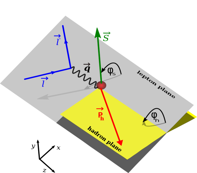
Figure 1: Definition of azimuthal angles (), lepton and hadron scattering planes
in semi inclusive deep inelastic scattering.
here, . The invariant mass of electron-target system is
and then we have . The virtual photon-target invariant mass is
defined as . Using Sudakov decomposition, the four momenta of
the initial gluon and the final hadron are
(6)
(7)
where, is the longitudinal momentum fraction, and .
Mass of the is denoted with . In line with Ref. Pisano et al. (2013) , we assume that
generalized factorization theorem allows to factorize the unpolarized differential cross section as
(8)
The leptonic tensor is given by
(9)
The gluon-gluon correlator, , describes the hadron to parton
transition
which is parametrized in terms of eight TMDs at leading twist. The gluon correlator is defined
for unpolarized and transversely polarized hadron respectively as below Mulders and Rodrigues (2001)
(10)
(11)
where is the
transverse metric tensor. Here we have kept only the part of the hadronic tensor for transverse polarization, that contributes to the Sivers asymmetry. and represent the unpolarized and
linearly polarized gluon distribution functions inside the unpolarized hadron respectively. , gluon Sivers function, describes the density of unpolarized gluons inside the transversely polarized
hadron.
The only LO subprocess for production is .
In Eq.(II), is the amplitude of
production. production mechanism, for instance, contains both perturbative and
nonperturbative regimes which need to be separated out systematically. We employ the COM to calculate
the amplitude of bound state.
The detailed calculation is discussed in the Appendix. In COM framework, initially
heavy quark pair produced in a definite quantum state which can be calculated using perturbation theory
up to a fixed order in . The long distance matrix element (LDME), , contains the transition probability of production from heavy
quark pair. The momentum conservation delta function can be decomposed as
(12)
The phase space factors in Eq.(II) can be written as follows
(13)
The differential cross section can be expressed in terms of TMDs by substituting parameterization of
gluon correlator, the leptonic tensor and Eq.(65)-(69) in Eq.(II). Using
Eq.(9)-(13) and after integrating with respect
to and , one obtains
(14)
with correction . The azimuthal angle of the initial
gluon transverse momentum is denoted with . For obtaining Eq.(14), is understood
where is the azimuthal angle of the . In Eq.(14), only the unpolarized gluon
contribution is
taken into
consideration. The effect of linearly
polarized gluon contribution will be discussed in the Sec.IV.
We define and as
(15)
(16)
with . does not contribute to the Sivers asymmetry.
The numerical values of the different states LDME are taken from Ref. Mukherjee and Rajesh (2017), Set-I in
Table-I.
Following Ref. Anselmino
et al. (2005b), the numerator term of the Sivers asymmetry is
given below when the target proton is transversely polarized
(17)
The gluon Sivers function
as per Trento convention is given by Bacchetta et al. (2004)
(18)
The scale dependency in the definition of TMD is suppressed in this section. The denominator term is given by
(19)
where the GSF describes the probability of finding an unpolarized gluon
inside a transversely polarized proton which is defined as
(20)
III Evolution of TMDs
In this section the evolution of TMDs is studied.
It is generally assumed that the unpolarized gluon TMDs obey the Gaussian distribution. The
Gaussian parameterization of unpolarized TMD is given by
(21)
Here, and dependencies of the TMD are factorized. is the collinear PDF
which is measured at the scale (mass of ). The collinear PDF obeys the
Dokshitzer-Gribov-Lipatov-Altarelli-Parisi (DGLAP) scale evolution.
We choose a frame where the polarized proton is moving along axis with momentum and is
transversely polarized with . The transverse momentum of the
is
(22)
where, and are the azimuthal angles which are defined in Figure 1.
The parameterization of GSF is given by D’Alesio et al. (2015); Anselmino et al. (2017)
(23)
here
(24)
is defined as follows
(25)
Therefore, the dependent part of Sivers function can now be written as
(26)
where we defined
(27)
The GSF has been extracted first time in pion production at RHIC Adare et al. (2014) by D’Alesio et al.
D’Alesio et al. (2015). In this analysis D’Alesio et al. (2015), the best fit parameter sets are denoted with SIDIS1 and
SIDIS2. Recently, M. Anselmino et al. Anselmino et al. (2017) have extracted the quark and
anti-quark Sivers function from latest SIDIS data. However, GSF has not been extracted yet from SIDIS
data. Therefore, in order to estimate the asymmetry, best fit
parameters of Sivers function corresponding to and quark will be used in
the following parameterizations Boer and Vogelsang (2004) :
(28)
We call the parameterization (a) and (b) as BV-a and BV-b respectively. The best fit parameters are
tabulated in Table 1.
We use the nonuniversality property of Sivers function for only SIDIS1 and SIDIS2 parameters since these
parameters are extracted in DY process Echevarria et al. (2014)
(29)
Finally, we are in position to write the final expressions of Eq.(1) within DGLAP evolution
formalism.
Using Eq.(21)-(III), the weighted numerator part of Eq.(1) is
given by
(30)
and the denominator term as follows
(31)
Now, we adopt the framework implemented in Ref. Echevarria et al. (2014) to study the TMD evolution. In general,
TMDs
are
defined in impact parameter ()-space as below
(32)
and the inverse Fourier transformation is
(33)
Generally, TMDs depend on both renormalization scale () and auxiliary scale () which is
introduced
to regularize the light-cone divergences in TMD factorization formalism Collins (2013); Aybat et al. (2012b). Taking the
scale evolution with respect to
and the renormalization group (RG) and Collins-Soper (CS) equations are obtained. By solving these
equations one obtains
the TMD PDF expression which is evolved from the initial scale to final scale
Echevarria et al. (2014); Collins (2013); Aybat et al. (2012b); Echevarria et al. (2015)
(34)
Here, is the perturbative part. The nonperturbative part of
the TMDs is denoted with . The initial scale of the TMDs is
,
where with . The widely used
prescription
is adopted to avoid hitting the Landau pole by freezing the scale . Here,
when and when .
The perturbative evolution kernel is given by
(35)
where the anomalous dimensions are denoted with an respectively and
these have perturbative expansion that can be written as :
and
Here the anomalous dimension coefficients ,
and .
These coefficients are derived up to 3-loop level in Ref. Idilbi et al. (2006). The nonperturbative part is given
by
(36)
It is known that Aybat et al. (2012b) the derivative of Sivers function, , follow the same evolution as that of the unpolarized TMD. The TMD evolution equation
of unpolarized
gluon TMD PDF is
(37)
and derivative of gluon Sivers function is
(38)
The TMD density function at the initial scale, , can be written as the
convolution
of coefficient function times the regular collinear PDF Aybat et al. (2012b)
(39)
where is the perturbatively calculated coefficient function which is process independent.
is different for each type of TMD PDF.
The collinear PDF is probed at the scale rather than the scale
in contrast to the DGLAP evolution. The unpolarized and Sivers function TMDs in terms of collinear
PDF at leading order in are given by Aybat et al. (2012b); Echevarria et al. (2014)
(40)
(41)
where is the Qiu-Sterman function proportional to collinear
PDF Kouvaris et al. (2006)
(42)
where definition is given in Eq.(24). The numerical values of the free
parameters are estimated Echevarria et al. (2014) by global fit of SSA in SIDIS process from pion, kaons and
charged hadrons production at Jlab, HERMES and COMPASS, which are tabulated in Table 1.
However, only the and quark’s free parameters are extracted and gluon parameters are not known
yet. To estimate SSA we use two parameterizations as given in Eq.(III). We call the
parameterization (a) and (b) as TMD-a and TMD-b respectively.
The numerical values of best fit parameters are estimated Echevarria et al. (2014) at
, , and
with and .
The gluon Sivers function and it’s derivative are related by
Fourier transformation as below Aybat et al. (2012b)
(43)
and the unpolarized gluon TMD is given by
(44)
Using above expressions, the Eq.(17), including the weight factor and (19) in TMD evolution framework
can be written as follows
(45)
(46)
IV azimuthal asymmetry
Now, let’s consider the unpolarized process i.e., . Taking into account the linearly polarized gluons along with the unpolarized
gluons in the gluon correlator, the Eq.(14) can be
written as
(47)
with correction . The definitions of
and are given in Eq.(15) and Eq.(16) respectively. The and
are defined as below
(48)
(49)
The dependence of the cross section on azimuthal angle vanishes when intrinsic parton transverse
momentum . The asymmetry is defined as
Airapetian et al. (2013); Adolph et al. (2014)
(50)
To estimate the asymmetry, we need the parameterization of TMDs. For unpolarized TMD, we
follow the Gaussian parameterization as defined in Eq.(21). The widely used Gaussian
parameterization for linearly polarized gluon distribution function is given by Boer and Pisano (2012)
(51)
where, () is the parameter. The upper bound on is given by
Boer et al. (2011)
(52)
We consider GeV2 Boer and Pisano (2012) and
and Boer and Pisano (2012) for numerical estimation.
V Numerical Results
We have estimated the Sivers and asymmetries respectively in polarized and unpolarized
SIDIS processes using TMD factorization formalism at (JLab),
(HERMES), (COMPASS) and
(EIC). In this work, NRQCD color octet model (COM) is used
for production. The color octet states ,
,
and are taken into account for the LO subprocess
of charmonium production. and
are considered for and charm quark mass respectively. MSTW2008
Martin et al. (2009) is used for collinear PDFs.
The following experimental cuts are imposed on the integration variables in Eq.(14).
For COMPASS Adolph et al. (2017); Matoušek (2016),
, for HERMES Airapetian et al. (2009),
, for JLab Qian et al. (2011)
, and for EIC,
.
The weighted Sivers asymmetry for the kinematics of different experiments is shown
in Figure2
-5 as a function of and . The SSA is estimated both in DGLAP and
Collins-Soper-Sterman (CSS) TMD evolution approach which is shown in Figure2-5.
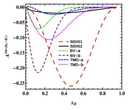
The figures convention is as follows. “SIDIS1” and “SIDIS2” represent the SSA obtained in DGLAP evolution approach by considering two sets
of best fit parameters SIDIS1 and SIDIS2 from Eq.(30) and (31). Similarly,
“BV-a” and “BV-b” represent the Sivers
asymmetry obtained by using Eq.(III) in DGLAP evolution. The obtained SSA in TMD evolution approach
using two
parameterizations from Eq.(III) is denoted by “TMD-a” and
“TMD-b”.
Recently extracted gluon Sivers function D’Alesio et al. (2015) from RHIC data and quark’s Sivers function
Anselmino et al. (2017) from latest SIDIS data have been employed in DGLAP evolution approach.
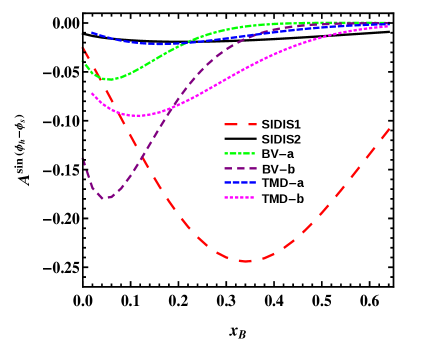
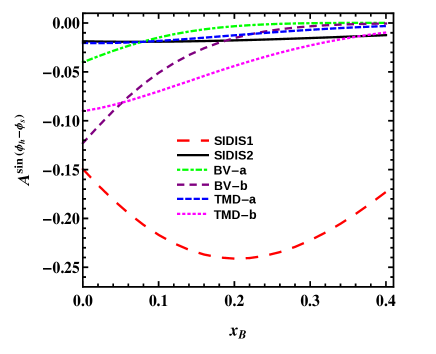
The SSA as a function of is negative, and is decreasing as the center of mass energy of the
experiment increasing, which is maximum around at JLab energy. Moreover, Sivers asymmetry as a
function of Bjorken variable () is negative and is maximum for SIDIS1 GSF parameters. Echevarria et
al. Echevarria et al. (2014), have extracted and quark’s
Sivers function by fitting data from JLab, HERMES and COMPASS within TMD evolution formalism. We use
best fit parameters of these for gluon
Sivers function as defined in Eq.(III) in CSS TMD evolution approach. Sivers asymmetry with
respect to obtained from SIDIS1 parameters is more at JLab and HERMES whereas SSA obtained from
BV-b set parameters is dominant at COMPASS and EIC experiments. Basically, SSA is proportional to gluon
Sivers function which is considered as
an average of and quark’s -dependent normalization in TMD-a
parameterization.
The sign of the asymmetry depends on relative magnitude of and and these have opposite sign which
can be observed in Table 1. Note that our kinematics is different from previous works in
Godbole et al. (2012, 2013, 2015), which also affects the sign.
The magnitude of is comparable but slightly dominant compared to
at EIC . Therefore, the estimated Sivers asymmetry as a function of
using TMD-a parameters for EIC experiment is almost zero and positive. For JLab experiment, the
estimated Sivers asymmetry by all the parameterizations except SIDIS1 is almost close to zero.
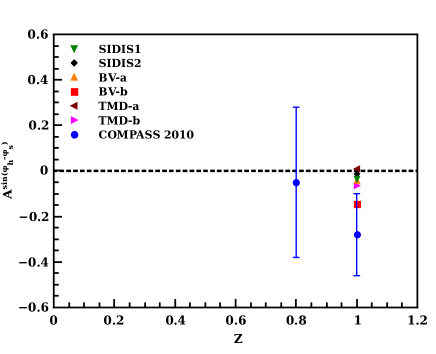
The delta function in Eq.(12) implies that (LO). In Figure 6, the obtained
Sivers asymmetry at is compared with COMPASS data Matoušek (2016). Interestingly, all the
set of parameters give negative asymmetry. However, estimated SSA with BV-b set of parameters is
within the error bar of the experiment. In Ref. Adolph et al. (2017), negative gluon Sivers asymmetry with more than two
standard deviation, , is reported in SIDIS process based on Monte carlo
simulation analysis. As stated before, it is expected that the Sivers
function has different sign in DY and SIDIS process, which comes from the gauge link. Sivers function in SIDIS has
been extracted by COMPASS Adolph et al. (2017); Matoušek (2016), HERMES Airapetian et al. (2009) and
JLab Qian et al. (2011) collaboration. However, information about the DY Sivers function has not been
explored, since polarized DY process has not been measured ever. Only very recently, data is available in DY process
Adamczyk et al. (2016). Anselmino et al. Anselmino et al. (2017)
have first time attempted to study the nonuniversality signature i.e., sign change of Sivers function,
however, they could not draw a definite conclusion about it due to poor data, although data for
production seem to favor the sign change.
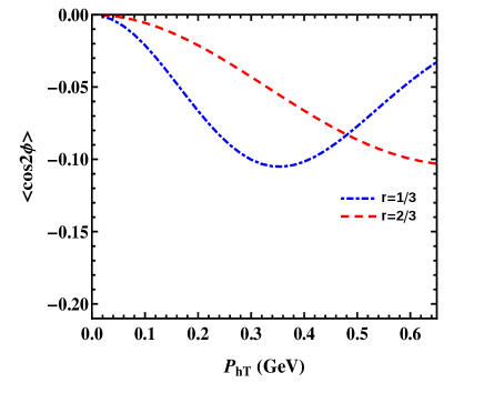
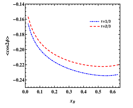
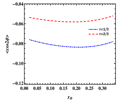
The asymmetry is shown in Figure 7-10 as a function of
and for and . To obtain asymmetry, the Gaussian parameterizations
for unpolarized and linearly polarized gluon distribution functions are used, as defined in
Eq.(21) and (51). Until now, experimental investigation has not been done to extract the
unknown Boer-Mulders function, . In Ref. Mukherjee and Rajesh (2016, 2017), the
effect of on the unpolarized differential cross section of production in
collision is explored. The production in unpolarized collision process is also a reliable channel to probe the
by measuring asymmetry.
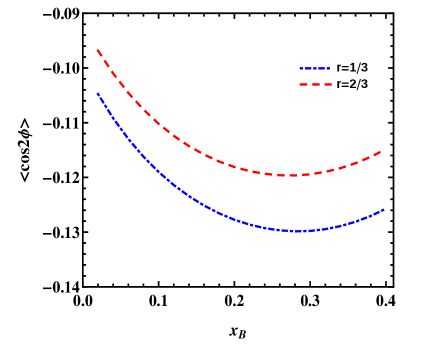
It is obvious from Eq.(48) that the negative asymmetry as function of and
is obtained due to the dominant contribution of state compared to the other states
(, and ).
asymmetry as a function of is almost same
for all the experiments, however, maximum value of decreases with .
The maximum of asymmetry as a function of is observed at EIC experiment.
(a)
(b)
Figure 2: Single spin asymmetry in
process as function of
(a) (left panel) and (b) (right panel) at GeV (EIC) using DGLAP (SIDIS1, SIDIS2,
BV-a and BV-b) and TMD (TMD-a and TMD-b) evolution approaches. The integration ranges are GeV,
and .
(a)
(b)
Figure 3: Single spin asymmetry in
process as function of
(a) (left panel) and (b) (right panel) at GeV (COMPASS) using DGLAP (SIDIS1, SIDIS2,
BV-a and BV-b) and TMD (TMD-a and TMD-b) evolution approaches. The integration ranges are GeV,
and .
(a)
(b)
Figure 4: Single spin asymmetry in
process as function of
(a) (left panel) and (b) (right panel) at GeV (HERMES) using DGLAP (SIDIS1, SIDIS2,
BV-a and BV-b) and TMD (TMD-a and TMD-b) evolution approaches. The integration ranges are GeV,
and
.
(a)
(b)
Figure 5: Single spin asymmetry in
process as function of
(a) (left panel) and (b) (right panel) at GeV (JLab) using DGLAP (SIDIS1, SIDIS2,
BV-a and BV-b) and
TMD (TMD-a and TMD-b) evolution approaches. The integration ranges are GeV,
and
.Figure 6: Single spin asymmetry in
process at with GeV (COMPASS) using DGLAP (SIDIS1, SIDIS2, BV-a and BV-b) and
TMD (TMD-a and TMD-b) evolution approaches. The integration ranges are GeV, and
. Data from Matoušek (2016).
(a)
(b)
Figure 7: asymmetry in
process as function of
(a) (left panel) and (b) (right panel) at GeV (EIC). The integration ranges
are GeV, and .
(a)
(b)
Figure 8: asymmetry in
process as function of (a) (left panel) and (b) (right panel) at GeV
(COMPASS). The integration ranges are GeV, and .
(a)
(b)
Figure 9: asymmetry in
process as function of (a) (left panel) and (b) (right panel) at GeV
(HERMES). The integration ranges are GeV, and .
(a)
(b)
Figure 10: asymmetry in
process as function of (a) (left panel) and (b) (right panel) at GeV
(JLab). The integration ranges are GeV, and .
VI Conclusion
We have calculated the Sivers and asymmetries in the production of in
polarized and unpolarized collision respectively. production
process gives direct access to the gluon Sivers function at leading order through the channel
. We used the NRQCD based color octet model and a formalism based on
TMD factorization. Sizable negative Sivers asymmetry is observed in production. The estimated
SSA at is compared
with COMPASS data and is in considerable agreement. We investigated the effect of TMD evolution on the
Sivers asymmetry. Moreover, Sizable asymmetry is obtained in unpolarized SIDIS process
which allows to probe the Boer-Mulders function, . Thus the asymmetries in the polarized
and unpolarized SIDIS processes are important observables to give valuable information on the gluon
Sivers function and linearly polarized gluon TMD respectively. Further work would involve taking into
account
higher order corrections to the asymmetry, where effect of the charmonium production mechanism is likely to
play an important role.
Acknowledgment
We would like to thank Mauro Anselmino for fruitful discussion during his stay at IIT Bombay. Cristian
Pisano is thanked for useful discussion.
*
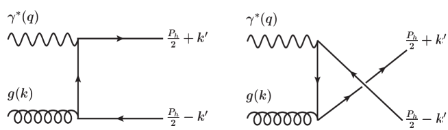
Appendix: LO amplitude of
Figure 11: Feynman diagrams for process.
As per Ref. Baier and Ruckl (1983); Boer and Pisano (2012), the amplitude of the quarkonium bound state can be written as
bellow
(53)
where is the relative momentum of the heavy quark in the quarkonium rest frame.
The eigenfunction of the orbital angular momentum is . We follow the similar
calculation as reported in Boer and Pisano (2012), hence only the important steps are presented below and for
more details Ref.Boer and Pisano (2012) is preferred. From
Figure11, the amplitude of heavy quark pair is given by
(54)
The sum over the SU(3) Clebsch-Gordan coefficients project out the color state of pair either it
is in color singlet or octet state, and are defined as
for color singlet and color octet states respectively.
is the SU(3) Gell-Mann matrix. Charm quark and quarkonium bound state masses are denoted with
and respectively.
The excluded external legs in Eq.(54) are absorbed in the spin projection operator which is given by
(55)
bear with for singlet () state and
for triplet () state. Here spin polarization vector of the system is denoted with
. The Taylor expansion around in Eq.(53) gives the -wave
and -wave amplitudes. The first term in the expansion is -wave amplitude
(56)
and
(57)
The derivative term in the expansion of Eq.(53) is the -wave amplitude
(58)
(59)
and
(60)
The definitions of and are obtained from Eq.(54) which are given by
(61)
(62)
Here and are the radial wave function and its derivative at the origin, and have the
following relation with LDME Ko et al. (1996)
(63)
(64)
After taking the trace one obtains the following amplitude expressions for -wave and -wave states
(65)
(66)
(67)
(68)
(69)
References
Klem et al. (1976)
R. D. Klem,
J. E. Bowers,
H. W. Courant,
H. Kagan,
M. L. Marshak,
E. A. Peterson,
K. Ruddick,
W. H. Dragoset,
and J. B.
Roberts, Phys. Rev. Lett.
36, 929 (1976).
Bunce et al. (1976)
G. Bunce et al.,
Phys. Rev. Lett. 36,
1113 (1976).
Adams et al. (1991a)
D. L. Adams et al.
(E704, E581), Phys. Lett.
B261, 201
(1991a).
Adams et al. (1991b)
D. L. Adams et al.
(FNAL-E704), Phys. Lett.
B264, 462
(1991b).
Arsene et al. (2008)
I. Arsene et al.
(BRAHMS), Phys. Rev. Lett.
101, 042001
(2008), eprint 0801.1078.
Arnold et al. (2009)
S. Arnold,
A. Metz, and
M. Schlegel,
Phys. Rev. D79,
034005 (2009), eprint 0809.2262.
Boer et al. (1997)
D. Boer,
R. Jakob, and
P. J. Mulders,
Nucl. Phys. B504,
345 (1997), eprint hep-ph/9702281.
Anselmino et al. (2007)
M. Anselmino,
M. Boglione,
U. D’Alesio,
A. Kotzinian,
F. Murgia,
A. Prokudin, and
C. Turk,
Phys. Rev. D75,
054032 (2007), eprint hep-ph/0701006.
Efremov and Teryaev (1982)
A. V. Efremov and
O. V. Teryaev,
Sov. J. Nucl. Phys. 36,
140 (1982), [Yad.
Fiz.36,242(1982)].
Efremov and Teryaev (1985)
A. V. Efremov and
O. V. Teryaev,
Phys. Lett. B150,
383 (1985).
Qiu and Sterman (1991)
J.-w. Qiu and
G. F. Sterman,
Phys. Rev. Lett. 67,
2264 (1991).
Qiu and Sterman (1999)
J.-w. Qiu and
G. F. Sterman,
Phys. Rev. D59,
014004 (1999), eprint hep-ph/9806356.
Kanazawa and Koike (2000)
Y. Kanazawa and
Y. Koike,
Phys. Lett. B478,
121 (2000), eprint hep-ph/0001021.
Kouvaris et al. (2006)
C. Kouvaris,
J.-W. Qiu,
W. Vogelsang,
and F. Yuan,
Phys. Rev. D74,
114013 (2006), eprint hep-ph/0609238.
Eguchi et al. (2007)
H. Eguchi,
Y. Koike, and
K. Tanaka,
Nucl. Phys. B763,
198 (2007), eprint hep-ph/0610314.
Kanazawa et al. (2014)
K. Kanazawa,
Y. Koike,
A. Metz, and
D. Pitonyak,
Phys. Rev. D89,
111501 (2014), eprint 1404.1033.
Sivers (1990)
D. W. Sivers,
Phys. Rev. D41,
83 (1990).
Airapetian et al. (2005)
A. Airapetian
et al. (HERMES),
Phys. Rev. Lett. 94,
012002 (2005), eprint hep-ex/0408013.
Airapetian et al. (2009)
A. Airapetian
et al. (HERMES),
Phys. Rev. Lett. 103,
152002 (2009), eprint 0906.3918.
Adolph et al. (2012)
C. Adolph et al.
(COMPASS), Phys. Lett.
B717, 383 (2012),
eprint 1205.5122.
Qian et al. (2011)
X. Qian et al.
(Jefferson Lab Hall A), Phys. Rev.
Lett. 107, 072003
(2011), eprint 1106.0363.
Zhao et al. (2014)
Y. X. Zhao et al.
(Jefferson Lab Hall A), Phys.
Rev. C90, 055201
(2014), eprint 1404.7204.
Anselmino
et al. (2009a)
M. Anselmino,
M. Boglione,
U. D’Alesio,
A. Kotzinian,
S. Melis,
F. Murgia,
A. Prokudin, and
C. Turk,
Eur. Phys. J. A39,
89 (2009a), eprint 0805.2677.
Anselmino
et al. (2009b)
M. Anselmino,
M. Boglione,
U. D’Alesio,
S. Melis,
F. Murgia, and
A. Prokudin,
Phys. Rev. D79,
054010 (2009b),
eprint 0901.3078.
Anselmino
et al. (2005a)
M. Anselmino,
M. Boglione,
U. D’Alesio,
A. Kotzinian,
F. Murgia, and
A. Prokudin,
Phys. Rev. D72,
094007 (2005a),
[Erratum: Phys. Rev.D72,099903(2005)],
eprint hep-ph/0507181.
Godbole et al. (2012)
R. M. Godbole,
A. Misra,
A. Mukherjee,
and V. S.
Rawoot, Phys. Rev.
D85, 094013
(2012), eprint 1201.1066.
Godbole et al. (2013)
R. M. Godbole,
A. Misra,
A. Mukherjee,
and V. S.
Rawoot, Phys. Rev.
D88, 014029
(2013), eprint 1304.2584.
Godbole et al. (2015)
R. M. Godbole,
A. Kaushik,
A. Misra, and
V. S. Rawoot,
Phys. Rev. D91,
014005 (2015), eprint 1405.3560.
Boer et al. (2016)
D. Boer,
P. J. Mulders,
C. Pisano, and
J. Zhou,
JHEP 08, 001
(2016), eprint 1605.07934.
D’Alesio et al. (2017)
U. D’Alesio,
F. Murgia,
C. Pisano, and
P. Taels
(2017), eprint 1705.04169.
Mukherjee and Rajesh (2016)
A. Mukherjee and
S. Rajesh,
Phys. Rev. D93,
054018 (2016), eprint 1511.04319.
Mukherjee and Rajesh (2017)
A. Mukherjee and
S. Rajesh,
Phys. Rev. D95,
034039 (2017), eprint 1611.05974.
Cacciari and Kramer (1996)
M. Cacciari and
M. Kramer, 1,
Phys. Rev. Lett. 76,
4128 (1996), eprint hep-ph/9601276.
Bodwin et al. (1995)
G. T. Bodwin,
E. Braaten, and
G. P. Lepage,
Phys. Rev. D51,
1125 (1995), [Erratum: Phys.
Rev.D55,5853(1997)], eprint hep-ph/9407339.
D’Alesio et al. (2015)
U. D’Alesio,
F. Murgia, and
C. Pisano,
JHEP 09, 119
(2015), eprint 1506.03078.
Aybat et al. (2012a)
S. M. Aybat,
A. Prokudin, and
T. C. Rogers,
Phys. Rev. Lett. 108,
242003 (2012a),
eprint 1112.4423.
Aybat et al. (2012b)
S. M. Aybat,
J. C. Collins,
J.-W. Qiu, and
T. C. Rogers,
Phys. Rev. D85,
034043 (2012b),
eprint 1110.6428.
Aybat and Rogers (2011)
S. M. Aybat and
T. C. Rogers,
Phys. Rev. D83,
114042 (2011), eprint 1101.5057.
Collins and Rogers (2017)
J. Collins and
T. C. Rogers,
Phys. Rev. D96,
054011 (2017), eprint 1705.07167.
Arneodo et al. (1987)
M. Arneodo et al.
(European Muon), Z. Phys.
C34, 277 (1987).
Breitweg et al. (2000)
J. Breitweg et al.
(ZEUS), Phys. Lett.
B481, 199 (2000),
eprint hep-ex/0003017.
Falciano et al. (1986)
S. Falciano et al.
(NA10), Z. Phys.
C31, 513 (1986).
Guanziroli et al. (1988)
M. Guanziroli
et al. (NA10), Z.
Phys. C37, 545
(1988).
Airapetian et al. (2013)
A. Airapetian
et al. (HERMES),
Phys. Rev. D87,
012010 (2013), eprint 1204.4161.
Adolph et al. (2014)
C. Adolph et al.
(COMPASS), Nucl. Phys.
B886, 1046
(2014), eprint 1401.6284.
Barone et al. (2010)
V. Barone,
S. Melis, and
A. Prokudin,
Phys. Rev. D81,
114026 (2010), eprint 0912.5194.
Barone et al. (2015)
V. Barone,
M. Boglione,
J. O. Gonzalez Hernandez,
and S. Melis,
Phys. Rev. D91,
074019 (2015), eprint 1502.04214.
Barone et al. (2007)
V. Barone,
Z. Lu, and
B.-Q. Ma,
Eur. Phys. J. C49,
967 (2007), eprint hep-ph/0612350.
Pisano et al. (2013)
C. Pisano,
D. Boer,
S. J. Brodsky,
M. G. A. Buffing,
and P. J.
Mulders, JHEP
10, 024 (2013),
eprint 1307.3417.
Mulders and Rodrigues (2001)
P. J. Mulders and
J. Rodrigues,
Phys. Rev. D63,
094021 (2001), eprint hep-ph/0009343.
Anselmino
et al. (2005b)
M. Anselmino,
M. Boglione,
U. D’Alesio,
A. Kotzinian,
F. Murgia, and
A. Prokudin,
Phys. Rev. D71,
074006 (2005b),
eprint hep-ph/0501196.
Bacchetta et al. (2004)
A. Bacchetta,
U. D’Alesio,
M. Diehl, and
C. A. Miller,
Phys. Rev. D70,
117504 (2004), eprint hep-ph/0410050.
Anselmino et al. (2017)
M. Anselmino,
M. Boglione,
U. D’Alesio,
F. Murgia, and
A. Prokudin,
JHEP 04, 046
(2017), eprint 1612.06413.
Adare et al. (2014)
A. Adare et al.
(PHENIX), Phys. Rev.
D90, 012006
(2014), eprint 1312.1995.
Boer and Vogelsang (2004)
D. Boer and
W. Vogelsang,
Phys. Rev. D69,
094025 (2004), eprint hep-ph/0312320.
Echevarria et al. (2014)
M. G. Echevarria,
A. Idilbi,
Z.-B. Kang, and
I. Vitev,
Phys. Rev. D89,
074013 (2014), eprint 1401.5078.
Echevarria et al. (2015)
M. G. Echevarria,
T. Kasemets,
P. J. Mulders,
and C. Pisano,
JHEP 07, 158
(2015), eprint 1502.05354.
Idilbi et al. (2006)
A. Idilbi,
X.-d. Ji, and
F. Yuan,
Nucl. Phys. B753,
42 (2006), eprint hep-ph/0605068.
Boer and Pisano (2012)
D. Boer and
C. Pisano,
Phys. Rev. D86,
094007 (2012), eprint 1208.3642.
Boer et al. (2011)
D. Boer,
S. J. Brodsky,
P. J. Mulders,
and C. Pisano,
Phys. Rev. Lett. 106,
132001 (2011), eprint 1011.4225.
Martin et al. (2009)
A. D. Martin,
W. J. Stirling,
R. S. Thorne,
and G. Watt,
Eur. Phys. J. C63,
189 (2009), eprint 0901.0002.
Adolph et al. (2017)
C. Adolph et al.
(COMPASS) (2017),
eprint 1701.02453.
Matoušek (2016)
J. Matoušek
(COMPASS), J. Phys. Conf. Ser.
678, 012050
(2016).
Adamczyk et al. (2016)
L. Adamczyk et al.
(STAR), Phys. Rev. Lett.
116, 132301
(2016), eprint 1511.06003.
Baier and Ruckl (1983)
R. Baier and
R. Ruckl, Z.
Phys. C19, 251
(1983).
Ko et al. (1996)
P. Ko,
J. Lee, and
H. S. Song,
Phys. Rev. D54,
4312 (1996), [Erratum: Phys.
Rev.D60,119902(1999)], eprint hep-ph/9602223.
 (b)
(b)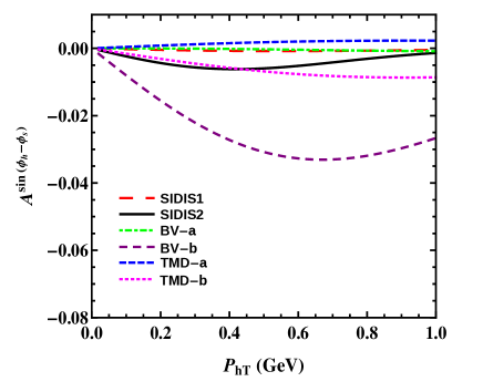
 (b)
(b)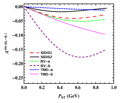
 (b)
(b)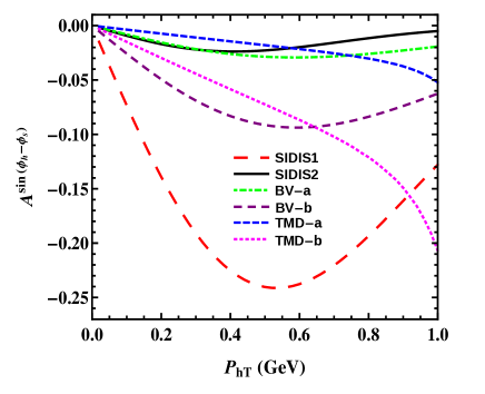
 (b)
(b)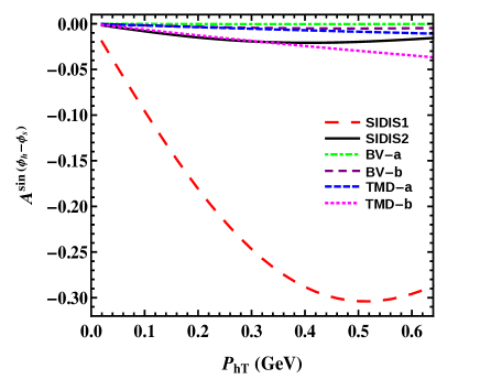
 (b)
(b)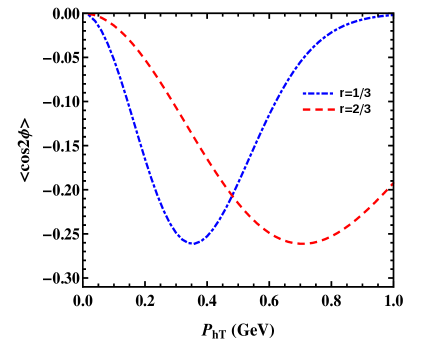
 (b)
(b)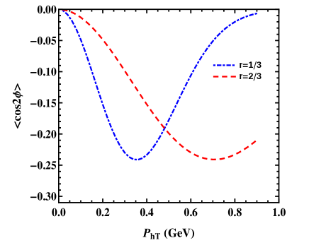
 (b)
(b)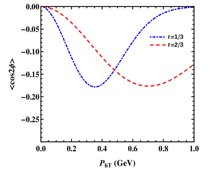
 (b)
(b)