Proton-proton hollowness at the LHC from inverse scattering

Abstract

Parameterizations of the pp scattering data at the LHC collision energies indicate a hollow in the inelasticity profile of the pp interaction, with less absorption for head-on collisions than at a non-zero impact parameter. We show that some qualitatively unnoticed features may be unveiled by a judicious application of the inverse scattering problem in the eikonal approximation and interpretation within an optical potential model. The hollowness effect is magnified in a 3D picture of the optical potential, and will presumably be enhanced at yet higher energies. Moreover, in 3D it sets in at much smaller energies than at the LHC. We argue that hollowness in the impact parameter is a quantum effect, relying on the build-up of the real part of the eikonal scattering phase and its possible passage through $\pi/2$. We also show that it precludes models of inelastic collisions where inelasticity is obtained by naive folding of partonic densities.

I Introduction

The main purpose of scattering experiments is to unveil the underlying structure of the colliding particles. However, there is always a limiting resolution of the relative de Broglie wavelength $\Delta r=1/p_{\rm CM}\sim 2/\sqrt{s}$, which effectively coarse-grains both the interaction between colliding particles and their structure as seen in the collision process. Of course, as the energy increases, new production channels open and inelasticities become important, but this does not change the overall picture even if the elastic scattering is regarded as the diffractive shadow of the particle production. Besides the early cosmic rays investigations in the mid 50’s williams1955highII reporting a surprisingly too large cross section compared to accelerator extrapolations williams1955highI , the accumulation of more precise scattering data since the early 60’s until the ISR experiments in the 70’s (see, e.g., Amaldi:1979kd for a compilation), has been modifying our picture of the nucleon along the years Block:1984ru ; Cheng:1987ga ; Matthiae:1994uw ; Barone:2002cv ; Dremin:2012ke with the deceiving result that the asymptotic regime may still be further away than hitherto assumed. The shortest wavelengths ever available in a terrestrial laboratory are achieved in the current and upcoming proton-proton (pp) scattering at the CERN Large Hadron Collider, with $\sqrt{s}=7-14{\rm~{}TeV}$ corresponding to $\Delta r\sim 0.001{\rm~{}fm}=1{\rm~{}am}$, a tiny length compared to the conventional proton size. From the point of view of the relative distance, the maximum momentum transfer $t=-\vec{q}_{\perp}^{2}$ samples the smallest impact parameter $\Delta b=1/q_{\perp}$. The succinct summary of the whole development is that, historically, protons become larger, edgier and blacker as the energy of the collision is being increased.

In a recent communication Arriola:2016bxa , we have analyzed the TOTEM data Antchev:2013gaa for the pp collisions at $\sqrt{s}=7$ TeV in terms of the so-called on-shell optical potential. A striking result is that there appears to be more inelasticity when the two protons are at about half a fermi traverse separation than for head-on collisions: a hollow is developed in the pp inelasticity profile. This counterintuitive finding has also been noticed by several other authors Alkin:2014rfa ; Dremin:2014eva ; Dremin:2014spa ; Anisovich:2014wha ; Dremin:2016ugi . As we will show, it actually precludes a probabilistic geometric explanation of the pp inelasticity profile based on folding of one-body partonic densities. We note that microscopic realization of the hollowness effect has been offered within a hot spot Glauber model Albacete:2016pmp for the elastic pp amplitude.

In the present paper we largely extend the findings of Ref. Arriola:2016bxa . We analyze the problem from an inverse-scattering point of view, utilizing the standard optical potential in the eikonal approximation (not to be confused with the on-shell one, see below). The eikonal method is justified for sufficiently small impact parameters, $b<3{\rm~{}fm}$, and for the CM energies of the system $\sqrt{s}>20{\rm~{}GeV}$. The 3D hole in the optical potential emerges already at $\sqrt{s}\sim 1{\rm~{}TeV}$, well below the present LHC energies. We note that the hollowness effect becomes less visible in the 2D inelasticity profile in the impact parameter space, where geometrically the 3D hole is covered up by the accumulated longitudinal opacity of two colliding protons.

We take no position on the particular underlying dynamics of the system. Instead, we rely on accepted and working parameterizations of the NN scattering amplitude. For definiteness, we apply the modified Barger-Phillips amplitude 2 (MBP2) used in the comprehensive analysis of Fagundes et al. Fagundes:2013aja , where the implemented properties at low- and high values of $t$ are indeed supported by reasonable $\chi^{2}$ values and visual inspection vs data. It is thus fair to assume that these fits capture the essence of the scattering amplitude at any fixed energy and up to a certain $t_{\rm max}$. Correspondingly, the present experimental range covers impact parameters larger than $b_{\rm min}\sim 0.1{\rm~{}fm}$, which is the fiducial domain of the present study.

We use the well-established inverse scattering methods to determine the optical potential. This has the advantage of being free of dynamical assumptions, in particular, naive folding features assumed quite naturally by model calculations but which turn out to be hard to reconcile with the hollowness effect.

Finally, let us note that we will not make any separation other than single elastic channel from inelastic channels (being all the rest). Therefore the verification of the conjecture that the calculated elastic cross section includes diffraction, whereas the inelastic cross section only includes uncorrelated processes, as put forward in Refs. Lipari:2009rm ; Lipari:2013kta ; Fagundes:2015vba , will not be addressed in the present study.

II Mass squared approach with central optical potential

The NN elastic scattering amplitude has 5 complex Wolfenstein components, as it corresponds to scattering of identical spin 1/2 particles PhysRev.85.947 . Besides, at high energies, $\sqrt{s}\gg 2M_{N}$, both relativistic effects and inelasticities must be taken into account. In principle, a field theoretic description of particle production would require solving a multi-channel Bethe-Salpeter (BS) equation. Taking into account that most of the produced particles are pions, the maximum number of coupled channels involving just direct pion production $pp\to pp+n\pi$ necessary to preserve the (coupled channel) unitarity would involve at least $n^{\rm max}\sim(\sqrt{s}-2M_{N})/m_{\pi}$ channels. For ISR energies it corresponds to $n_{\rm ISR}^{\rm max}\sim 150-450$, whereas for the LHC energies $n_{\rm LHC}^{\rm max}\sim 5\times 10^{5}$. Such a huge number of channels prevents from the outset a direct coupled channel calculation. Another added difficulty is the incorporation of spin at these high energies, mainly because the experimental information is insufficient. Thus, as it is usually assumed in most calculations, at these high energies spin effects are fully neglected and a purely central type of interaction is taken.

An advantageous way to take into account inelasticities is to recourse to an optical potential where all inelastic channels are in principle integrated out. Even if all the particle production processes were known, an explicit construction for the huge number of channels has never been carried out, hence our approach is phenomenological, with the idea to deduce the optical potential directly from the data via an inverse scattering method. Because such a framework is currently not commonly used in high-energy physics, it is appropriate to review it here, providing in passing a justification on why we choose it.

The optical potential was first introduced to describe the inelastic neutron-nucleus scattering above the compound nucleus regime Fernbach:1949zz (typically in the $10-500{\rm~{}MeV}$ range). There, the concept of the black disk limit was first tested, along with the Fraunhofer diffraction pattern appearing as a shadow scattering effect. This work inspired Glauber’s seminal studies glauber1959high on the eikonal approximation, which is currently successfully applied to model the early stages of the ultra-relativistic heavy-ion collisions (see e.g. Florkowski:2010zz ). Serber serber1963theory ; serber1964scaling ; serber1964high provided an extension of the optical eikonal formalism to high energy particle physics. As it was shown by Omnes omnes1965optical , the simple assumption of a double spectral representation of the Mandelstam representation of the scattering amplitude suffices to justify the use of an optical potential. Cornwall and Ruderman cornwall1962mandelstam delineated a more precise definition of the optical potential, directly based in field theory and tracing its analytic properties from the causality requirement. Some further field theoretic discussions using the multichannel BS equation can be found in torgerson1966field ; arnold1967optical , and were early reviewed by Islam islam1972optical .

The simplest way of retaining relativity without solving a BS equation with a phenomenological optical potential is by using the so-called mass squared method, discussed by Allen, Payne, and Polyzou in an insightful paper Allen:2000xy . The idea is to postulate the total squared mass operator for the pp system as

$${\cal M}^{2}=P^{\mu}P_{\mu}\stackrel{{\scriptstyle CM}}{{=}}4(p^{2}+M_{N}^{2})+{\cal V},$$ (1)

where $P^{\mu}$ is the total four-momentum, CM indicates the center-of-mass frame, $p$ is the CM momentum of each nucleon, $M_{N}$ is the nucleon mass, and ${\cal V}$ represents the invariant (momentum-independent) interaction, whose form can be determined in the CM frame by matching to the non-relativistic limit with a non-relativistic potential $V(\vec{x})$. This allows one, after quantization, to write down the relativistic wave equation ${\cal\hat{M}}^{2}\Psi=s\Psi$, in the form of an equivalent non-relativistic Schrödinger equation Allen:2000xy

$$(-\nabla^{2}+U)\Psi=(s/4-M_{N}^{2})\Psi,$$ (2)

with the reduced potential $U=M_{N}V$. In essence, the invoked prescription corresponds to a simple rule where one may effectively implement relativity by just promoting the non-relativistic CM momentum to the relativistic CM momentum.

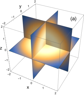
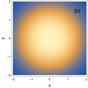
Figure 1: Projection of a sample spherically symmetric three-dimensional function (a) on two dimensions (b), as in Eq. (8). A shallow hollow present in (a) disappears in (b), where it is only reflected with a flatness on the central region.

As remarked by Omnes omnes1965optical , “one can always find an optical potential that fits any amplitude satisfying the Mandelstam analyticity assumptions”, and we apply a definite prescription to accomplish this goal. To account for inelasticity, we assume an energy-dependent and local phenomenological optical potential, $U(\vec{r};s)={\rm Re}\,U(\vec{r};s)+i{\rm Im}\,U(\vec{r};s)$, which can be obtained by fitting the scattering data. Due to causality, the optical potential in the $s$ channel satisfies a fixed-$r$ dispersion relation. Together with Eq. (2), it provides the necessary physical ingredients present in any field theoretic approach: relativity and inelasticity, consistent with analyticity. The potential $U$ appearing in Eq. (2) will be determined in the following via inverse scattering in the eikonal approximation for any value of $s$. To ease the notation, the $s$-dependence is suppressed below.

III On-shell optical potential and the eikonal approximation

Besides the “standard” potential $U$, the object we are going to use is the on-shell optical potential $W$, defined by a Low-type integral equation discussed, e.g., in cornwall1962mandelstam ; namyslowski1967relativistic ; Nieves:1999bx ; Arriola:2016bxa . From Eq. (2) we get for the probability flux

$$\oint_{r=R}\vec{d}S\cdot\vec{J}=\int_{r\leq R}d^{3}x\,{\rm Im}\,U(\vec{x})|\Psi(\vec{x})|^{2},$$ (3)

with $\vec{J}=\Psi^{*}(\vec{\nabla}\Psi)-(\vec{\nabla}\Psi^{*})\Psi$ denoting the probability current. The asymptotic behavior of the wave function is $\Psi(\vec{x})\to e^{i\vec{p}\cdot\vec{x}}+f(\hat{x}){e^{ipr}}/{r}$. It follows from the definition of the inelastic cross section that

$$\sigma_{T}-\sigma_{\rm el}\equiv\sigma_{\rm in}=-\frac{1}{p}\int d^{3}x\,{\rm Im}\,U(\vec{x})|\Psi(\vec{x})|^{2},$$ (4)

with shows that the density of inelasticity is proportional to the absorptive part of the optical potential times the square of the modulus of the wave function. One can now identify the on-shell optical potential as

$${\rm Im}\,W(\vec{x})={\rm Im}\,U(\vec{x})|\Psi(\vec{x})|^{2}.$$ (5)

In the eikonal approximation one has

$$\Psi(\vec{x})=\exp\left[ipz-\frac{i}{2p}\int_{-\infty}^{z}U(\vec{b},z^{\prime})dz^{\prime}\right],$$ (6)

thus

$${\rm Im}\,W(\vec{x})=p\frac{d}{dz}\exp\left[\frac{1}{p}\int_{-\infty}^{z}{\rm Im}U(\vec{b},z^{\prime})dz^{\prime}\right].$$ (7)

Upon $z$ integration,

$$-\frac{1}{p}\int_{-\infty}^{\infty}dz{\rm Im}\,W(\vec{b},z)=1-e^{-2{\rm Im}\chi(b)}\equiv n_{\rm in}(b),$$ (8)

where

$$\chi(b)=-\frac{1}{2p}\int_{-\infty}^{\infty}U(\sqrt{b^{2}+z^{2}})dz=-\frac{1}{p}\int_{b}^{\infty}\frac{rU(r)\,dr}{\sqrt{r^{2}-b^{2}}}$$

(9)

is the (complex) eikonal phase glauber1959high . Equation (7) is the standard result for the inelasticity profile $n_{\rm in}(b)$ in the eikonal approximation. Note that it links the imaginary part of the eikonal phase with the absorptive part of the on-shell optical potential $W$, hence the significance of this object in the present study.

The inverse scattering problem has been solved in newton1962construction and in the eikonal approximation in omnes1965optical (for a review see, e.g., buck1974inversion ). In our case the inversion is based on the fact that Eq. (9) is of a type of the Abel integral equation, hence the solution for the optical potential $U$ takes the simple form glauber1959high

$$U(r)=M_{N}V(r)=\frac{2p}{\pi}\int_{r}^{\infty}db\frac{\chi^{\prime}(b)}{\sqrt{b^{2}-r^{2}}},$$ (10)

which may be straightforwardly checked via direct substitution . Similarly, from Eq. (8) one obtains

$${\rm Im}W(r)=\frac{p}{\pi}\int_{r}^{\infty}db\frac{n_{\rm in}^{\prime}(b)}{\sqrt{b^{2}-r^{2}}}.$$ (11)

As the (complex) scattering phase may be obtained from the data parameterizations (see the following section), Eqs. (10) and (11) provide a simple way to obtain the corresponding optical potentials. An investigation of their behavior with the increasing collision energy is our principal goal.

Before going to the details of the next sections, let us comment on a simple geometric interpretation of formula (8). Suppose we have a spherically symmetric three-dimensional function with a lower density in the middle than in outer layers, as depicted in Fig. 1(a). If the hollow is not too deep, the projection of the function on two dimensions, as presented in Eq. (8), covers it up by the inclusion of the outer layers. In the example of Fig. 1(b) the central region is flat. Therefore the flatness of the inelasticity profile $n_{\rm in}(b)$ corresponds to a hollow in the imaginary part of the on-shell optical potential ${\rm Im}W(r)$. In other words, the three-dimensional objects as ${\rm Im}W(r)$ or $U(r)$ are more sensitive to exhibit a hollow than their corresponding 2D projections, i.e., the inelasticity profile or the eikonal phase.

IV Amplitudes and parameterization

The pp elastic scattering differential cross section is given by

$$\frac{d\sigma_{\rm el}}{dt}=\frac{\pi}{p^{2}}\frac{d\sigma_{\rm el}}{d\Omega}=\frac{\pi}{p^{2}}|f(s,t)|^{2}\,,$$ (12)

with the spinless partial wave expansion of the scattering amplitude

$$f(s,t)=\sum_{l=0}^{\infty}(2l+1)f_{l}(p)P_{l}(\cos\theta)$$ (13)

$$=\frac{p^{2}}{\pi}\int d^{2}b\,h(\vec{b},s)\,e^{i\vec{q}\cdot\vec{b}}=2p^{2}\int_{0}^{\infty}bdbJ_{0}(bq)h(b,s)\,,$$

where $t=-\vec{q}^{2}$ and $q=2p\sin(\theta/2)$ denotes the momentum transfer. The Coulomb effects can be neglected for $|t|>8\pi\alpha/\sigma_{T}$ ($\alpha\simeq 1/137.04$ is the fine structure constant) Block:1984ru . In the eikonal limit, justified for $pa\gg 1$ with $a$ standing for the range of the interaction, one has $bp=l+1/2+{\cal O}(s^{-1})$, hence the amplitude in the impact-parameter representation becomes

$$h(b,s)=\frac{i}{2p}\left[1-e^{i\chi(b)}\right]=f_{l}(p)+{\cal O}(s^{-1}),$$ (14)

whereas $P_{l}(\cos\theta)\to J_{0}(qb)$. Explicitly,

$$2ph(s,b)=\frac{1}{p}\int_{0}^{\infty}qdqJ_{0}(bq)f(s,-q^{2}).$$ (15)

The standard formulas for the total, elastic, and total inelastic cross sections read Blankenbecler:1962ez

$$\sigma_{T} = \frac{4\pi}{p}{\rm Im}f(s,0)=4p\int d^{2}b{\rm Im}h(\vec{b},s)$$ (16)

$$= 2\int d^{2}b\left[1-{\rm Re}\,e^{i\chi(b)}\right]\,,$$

$$\sigma_{\rm el} = \int d\Omega|f(s,t)|^{2}=4p^{2}\int d^{2}b|h(\vec{b},s)|^{2}$$ (17)

$$= \int d^{2}b|1-e^{i\chi(b)}|^{2}\,,$$

$$\sigma_{\rm in} \equiv \sigma_{T}-\sigma_{\rm el}=\int d^{2}bn_{\rm in}(b)$$ (18)

$$= \int d^{2}b\left[1-e^{-2{\rm Im}\chi(b)}\right]\,.$$

The inelasticity profile

$$n_{\rm in}(b)=4p{\rm Im}h(b,s)-4p^{2}|h(b,s)|^{2},$$ (19)

satisfies $n_{\rm in}(b)\leq 1$, conforming to unitarity and the probabilistic interpretation of absorption.

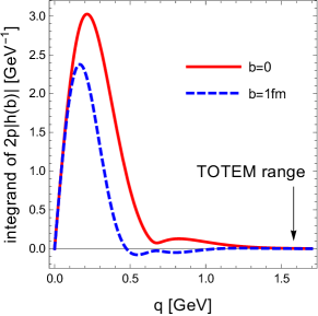
Figure 2: Absolute value of the integrand of the elastic amplitude from Eq. (15), $qJ_{0}(bq)|f(s,-q^{2})|/p$, plotted as a function of $q=\sqrt{-t}$ for two sample values of the impact parameter $b$. The amplitude $f(s,-q^{2})$ is taken from the parameterization (20) for $\sqrt{s}=7$ TeV. The arrow indicates the upper range of the TOTEM Antchev:2013gaa data.

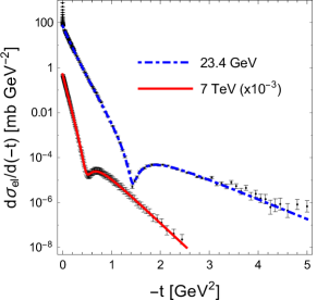
Figure 3: The differential elastic cross section in pp collisions from the MBP2 parametrization of Ref. Fagundes:2013aja (lines), compared to the ISR Amaldi:1979kd data at $\sqrt{s}=23.4$ GeV and the TOTEM Antchev:2013gaa data at $\sqrt{s}=7$ TeV.

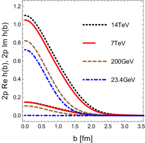
Figure 4: The imaginary (upper four curves) and real (lower four curves) parts of the eikonal amplitude multiplied with twice the CM momentum, $2ph(b)$, plotted as functions of the impact parameter $b$.

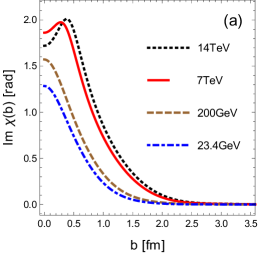
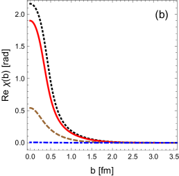
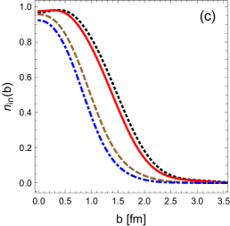
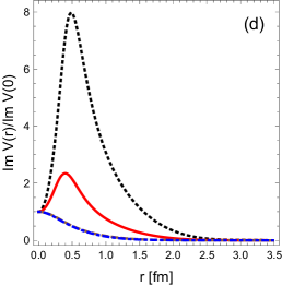
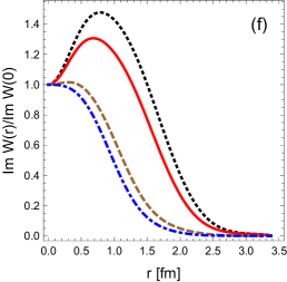
Figure 5: (a) Imaginary part of the eikonal phase $\chi(b)$, plotted as a function of $b$, for several collision energies. (b) Same as (a) but for the real part of the eikonal phase. (c) Same as (a) but for the inelasticity profile $n_{\rm in}(b)$. (d) Imaginary part of the optical potential $V(r)$ divided with ${\rm Im}V(0)$, plotted as a function of the radius $r$, for collision energies as in (a). (e) Same as (d) but for the real part of the optical potential. (e) Same as (d) but for the imaginary part of the on-shell optical potential $W(r)$ divided with ${\rm Im}W(0)$. The plots in the lower row are obtained, correspondingly, from the plots in the upper row via the transformations of Eqs. (10) or (11).

We use the parametrization of the pp scattering data provided by Fagundes et al. Fagundes:2013aja based in the Barger-Phillips analysis Phillips:1974vt motivated by the Regge asymptotics:

$${\cal A}(s,t) \equiv \frac{f(s,t)}{p}=\sum_{n}c_{n}(s)F_{n}(t)s^{\alpha_{n}(t)}$$ (20)

$$=\frac{i\sqrt{A}e^{\frac{Bt}{2}}}{\left(1-\frac{t}{t_{0}}\right)^{4}}+i\sqrt{C}e^{\frac{Dt}{2}+i\phi},$$

where the linear Regge trajectories $\alpha_{n}(t)=\alpha_{n}(0)+\alpha_{n}^{\prime}(0)t$ are assumed. Specifically, we take the MBP2 parametrization of Fagundes:2013aja , with the $s$-dependent parameters fitted separately to all known differential pp cross sections for $\sqrt{s}=23.4$, $30.5$, $44.6$, $52.8$, $62.0$, and $7000~{}{\rm GeV}$ with a reasonable accuracy of $\chi^{2}/{\rm d.o.f}\sim 1.2-4.7$. A typical quality of the fit can be appreciated from Fig. 3, where we show the comparison to the data at two sample collision energies from ISR Amaldi:1979kd at $\sqrt{s}=23.4$ GeV, and from the LHC (the TOTEM Collaboration Antchev:2013gaa ) at $\sqrt{s}=7$ TeV.

Table 1: Scattering observables for different CM energy values, obtained from the MBP2 parameterization Fagundes:2013aja with the inclusion of the $\rho$ parameter according to Eq. (22), compared to experimental vales (lower rows).

$\sqrt{s}$ [GeV]	$\sigma_{\rm el}$ [mb]	$\sigma_{\rm in}$ [mb]	$\sigma_{\rm T}$ [mb]	$B~{}[{\rm GeV}^{-2}]$	$\rho$
23.4	6.6	31.2	37.7	11.6	0.00
Amaldi:1979kd	6.7(1)	32.2(1)	38.9(2)	11.8(3)	0.02(5)
200	10.0	40.9	50.9	14.4	0.13
Aielli:2009ca ; Bueltmann:2003gq			54(4)	16.3(25)
7000	25.3	73.5	98.8	20.5	0.140
Antchev:2013gaa	25.4(11)	73.2(13)	98.6(22)	19.9(3)	0.145(100)

To be consistent with the experimental values of the $\rho(s)$ parameter, where

$$\rho(s)=\frac{{\rm Re}{\cal A}(s,0)}{{\rm Im}{\cal A}(s,0)},$$ (21)

we modify the amplitude of Eq. (20) be replacing it with

$${\cal A}(s,t)\to\frac{i+\rho(s)}{\sqrt{1+\rho(s)^{2}}}|{\cal A}(s,t)|,$$ (22)

which amounts to imposing a $t$-independent ratio of the real to imaginary part of the amplitude. Other prescriptions have been discussed in detail in Ref. Antchev:2016vpy . We have checked that our results are similar if we take the Bailly et al. Bailly:1987ki parametrization $\rho(s,t)=\rho_{0}(s)/(1-t/t_{0}(s))$, where $t_{0}(s)$ is the position of the diffractive minimum. Nevertheless, the results in the impact parameter representation do depend to some extent on the form of $\rho(s,t)$ Antchev:2016vpy and the issue is intimately related to the separation of the strong amplitude from the Coulomb part. As these problems extend beyond the goals of this paper, we explore here the simplest choice of Eq. (22).

Prescription (22) preserves the quality of the fits of Fig. 3, and in addition the experimental values for $\rho(s)$ are reproduced. For the explored below values of $\sqrt{s}=23.4$ GeV, 200 GeV, 7 TeV, and 14 TeV we use, correspondingly, $\rho=0$, 0.13, 0.14, and 0.135 (the last value is obtained via extrapolation). For completeness, we provide Table 1 with the numerical results where predictions of Eq. (22) are compared to the available experimental data.

Finally, we judge the accuracy of the eikonal approximation by checking that the ratio $|h(b,p)/f_{l}(p)|\sim 1$ to better than $0.1\%$ when $bp=l+\frac{1}{2}$ and for $\sqrt{s}\geq 17~{}{\rm GeV}$ and $b\leq 3~{}{\rm fm}$ for the MBP2 parameterization. The performance of the approximation improves with increasing collision energy.

Before passing to the results, we also test whether the range of the data at $\sqrt{s}=7$ TeV is sufficient to draw accurate conclusions for the quantities in the impact-parameter representation. It is indeed the case, as can be inferred from Fig. 2.

V Results

Our simple calculation consists of the following steps. First, with a given parametrization for $f(s,t)$ we find $h(b)$ via a numerical inverse Fourier-Bessel transform in Eq. (13). Then from Eq. (14) we obtain the eikonal phase and the quantities from Eq. (16-19), whereas the optical potentials follow from Eqs. (10,11). The relevant quantities are displayed in Figs. 4 and 5. A few characteristic features should be stressed.

First, we note from Fig. 4 that with an increasing collision energy from ISR via RHIC to the LHC, the real part of the eikonal scattering amplitude ${\rm Re}h(b)$, while remaining small, increases (in our model, simply, ${\rm Re}\,h(b)=\rho{\rm Im}\,h(b)$). At the LHC energies, it reaches $\sim 15\%$ percent of the dominant imaginary part.

The eikonal phase is presented in Figs. 5 (a, b). We can see that its imaginary part develops a dip at the origin at the LHC energies. Moreover, it achieves a very sizable positive real part, of the size of the imaginary part at the LHC.

The inelasticity profile $n_{\rm in}(b)$, Fig. 5 (c), flattens near the origin as the collision energy is being increased, and for the LHC develops a shallow minimum at $b=0$, whereas the maximum shifts to $b>0$. Note that by construction and in accordance to unitarity $n_{\rm in}(b)\leq 1$. The dip at $b=0$ is a symptom of the 2D hollowness effect, discussed in a greater detain in the next section.

Finally, we observe dips in the imaginary parts of both the optical potential $V(r)$, Fig. 5 (d), and the on-shell optical potential $W(r)$, Fig. 5 (f), appearing prominently with an increasings $s$ and displaying the hollowness effects in 3D.

VI The nature of the hollow

As the pp collision energy increases, the total inelastic cross section $\sigma_{\rm in}(s)$ grows. Moreover, as shown in the previous section, the inelasticity profile in the impact parameter flattens at the origin, or even develops a shallow minimum at sufficiently large $s$, as follows from Fig. 6. By simple geometric arguments, this flattening must correspond to a 3D hollow in the radial density of inelasticity, here interpreted as the on-shell optical potential ${\rm Im}W(r)$, cf. Eq. (8). In fact, for the collision energies above the lowest ISR case of $\sqrt{s}=24.3$ GeV the function ${\rm Im}W(r)$ exhibits a depletion at the origin – the hollow.

As depicted in the introductory Fig. 1, the “hollowness” effect is more pronounced when interpreted in 3D, i.e., via ${\rm Im}W(r)$, than in its 2D projection, namely $n_{\rm in}(b)$ (cf. Eq. (8)), since a 3D function is integrated over the longitudinal direction, which effectively covers up the hole.

Folding ideas have been implemented in microscopic models based on intuitive geometric interpretation Chou:1968bc ; Chou:1968bg ; Cheng:1987ga ; Bourrely:1978da ; Block:2015sea . Interestingly, the 3D hollowness effect cannot be reproduced by naive folding of inelasticities of uncorrelated partonic constituents. If $\Psi_{A}(x_{1},x_{2},x_{3},\dots)$ and $\Psi_{B}(x^{\prime}_{1},x^{\prime}_{2},x^{\prime}_{3},\dots)$ are the corresponding partonic wave functions of hadrons A and B, the single parton distributions are given by

$$\rho_{A}(\vec{x}_{1}) = \int d^{3}x_{2}d^{3}x_{3}\dots|\Psi_{A}(x_{1},x_{2},x_{3},\dots)|^{2},$$

$$\rho_{B}(\vec{x}_{1}^{\prime}) = \int d^{3}x^{\prime}_{2}d^{3}x^{\prime}_{3}\dots|\Psi_{B}(x^{\prime}_{1},x^{\prime}_{2},x^{\prime}_{3},\dots)|^{2}.$$ (23)

In a folding model, antisymmetry of the wave functions is neglected and the absorptive part of the potential, ${\rm Im}\,W(r)$, is proportional to the overlap integral

$$\langle\Psi_{A}\Psi_{B}|\sum_{i\in A,i^{\prime}\in B}w(\vec{x}_{i}-\vec{x}_{i^{\prime}}-\vec{r})|\Psi_{A}\Psi_{B}\rangle$$ (24)

$$= \int d^{3}y\rho_{A}(\vec{x}+\vec{r}/2)w(\vec{x}^{\prime}-\vec{x})\rho_{B}(\vec{x}-\vec{r}/2)\,.$$

where $w(\vec{x}-\vec{x}^{\prime})$ denotes the interaction among constituents belonging to different hadrons (we omit further possible indices). For identical hadrons, A=B, and at small $r$ we get

$${\rm Im}\,W(r) \propto \int d^{3}xd^{3}x^{\prime}\rho(\vec{x}^{\prime}+\vec{r}/2)w(\vec{x}^{\prime}-\vec{x})\rho(\vec{x}-\vec{r}/2)$$ (25)

$$= \int d^{3}yd^{3}y^{\prime}\rho(\vec{x})\rho(\vec{x}^{\prime})w(\vec{x}^{\prime}-\vec{x})$$

$$- \frac{1}{2}\int d^{3}xd^{3}x^{\prime}[\vec{r}\cdot\nabla\rho(\vec{y})]w(\vec{x}-\vec{x}^{\prime})[\vec{r}\cdot\nabla^{\prime}\rho(\vec{x}^{\prime})]$$

$$+ \dots,$$

For a positive $w(\vec{x}-\vec{x}^{\prime})$ both integrals are necessarily positive as can be seen by going to the Fourier space. This proves that if ${\rm Im}W(r)$ stems from a folding of densities with $w(\vec{x}-\vec{x}^{\prime})>0$, then it necessarily has a local maximum at $r=0$, in contrast to the phenomenological hollowness result. Folding models usually take $w(\vec{x}-\vec{x}^{\prime})\propto\delta(\vec{x}^{\prime}-\vec{x})$ Chou:1968bc ; Chou:1968bg ; Cheng:1987ga ; Bourrely:1978da ; Block:2015sea .

Note that the above conclusion holds for any wave functions $\Psi_{A,B}$, correlated or not. In particular, one may think of modeling collisions of objects empty in the middle (for instance, protons made as triangles of three constituents). If inelasticity were to be obtained via above density folding, even in this case the absorption would be strongest for head-on collisions.

Figure 6: The curvature of the inelasticity profile $n_{\rm in}(b)$ at $b=0$ plotted as a function of the collision energy. The minimum emerges at $\sqrt{s}\simeq 3$ TeV.

Likewise, the 2D hollowness cannot be obtained by folding structures in the impact parameter space, as for instance used in the models of Ref. Chou:1968bc ; Chou:1968bg ; Cheng:1987ga ; Bourrely:1978da ; Block:2015sea .

In our model one may give a simple criterion for $n_{\rm in}$ to develop a dip at the origin. Introducing the short-hand notation $k(b)=2p{\rm Im}\,h(b)$ we have immediately from Eqs. (19) and (22) the equality

$$n_{\rm in}(b)=k(b)-(1+\rho^{2})k(b)^{2}/2.$$ (26)

Differentiating with respect to $b^{2}$ one immediately finds that $d^{2}n_{\rm in}(b)/db^{2}$ at the origin is negative when

$$2p{\rm Im}h(0)>\frac{1}{1+\rho^{2}}\sim 1,$$ (27)

where the departure from 1 is at a level of $2\%$ at the LHC and smaller at lower collision energies.

One can make the following direct connection to the eikonal phase. From Eq. (14) we get immediately

$$2p{\rm Im}\,h(b)=1-\cos\left({\rm Re}\chi(b)\right)e^{-{\rm Im}\chi(b)},$$ (28)

hence $2p{\rm Im}h(0)>1$ (thus satisfying criterion (27)) when ${\rm Re}\chi(0)$ increases above $\pi/2$, whence

$$\cos({\rm Re}\chi(b))<0.$$ (29)

This is indeed the case in Fig. 5(b).

Recall that in the Glauber model glauber1959high of scattering of composite objects, the eikonal amplitudes of individual scatterers are additive, composing the full eikonal amplitude $\chi(b)$. Thus, in this quantum-mechanical framework, the monotonic change of $\chi(b)$ with the collision energy may be caused by the corresponding change of the eikonal amplitudes of the scatterers, or the increase of the number of scatterers (as expected from the growing number of gluons at increasing energies), or both. Thus a quantum nature of the scattering process is the alleged key to the understanding of the hollowness effect.

Finally, we show that the 2D flatness of the inelasticity profile $n_{\rm in}(b)$ at the origin implies the 3D hollowness in ${\rm Im}W(r)$. If $n_{\rm in}(b)$ is constant for $0<b\leq b_{0}$, then lower range of the integration in Eq. (11) starts from $b_{0}$ and the integral has no singularity for $r<b_{0}$. Direct inspection shows that the magnitude of ${\rm Im}W(r)$ grows with $r$, which corresponds to 3D hollowness.

VII The hollow and the edge

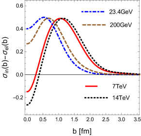
Figure 7: The edge function $\sigma_{T}(b)-2\sigma_{\rm el}(b)\equiv\sigma_{\rm in}(b)-\sigma_{\rm el}(b)$ as a function of the impact parameter for different energies.

The edge function, based on defining $\eta(b)=e^{-{\rm Im}\chi(b)}$ and analyzing the combination $\eta(b)(1-\eta(b))$, has been considered in Refs. Block:2014lna ; Block:2015sea (see, e.g., Ref. Rosner:2014nka for an interpretation in terms of string breaking). In the limit of a purely imaginary amplitudes the edge function can be interpreted as a combination of the unintegrated cross sections $\sigma_{T}(b)-2\sigma_{\rm el}(b)\equiv\sigma_{\rm in}(b)-\sigma_{\rm el}(b)$ (we use $\sigma_{\rm in}(b)\equiv n_{\rm in}(b)$). In the general case, with the real part of the eikonal phase present, it reads

$$\sigma_{\rm in}(b)-\sigma_{\rm el}(b)=2e^{-{\rm Im}\chi(b)}\left[\cos({\rm Re}\chi(b))-e^{-{\rm Im}\chi(b)}\right].$$

We show in Fig. 7 the edge functions at various collision energies resulting from our analysis. As we can see, the edge function becomes negative at the LHC energies for $b\lesssim 0.5{\rm fm}$ due to the same quantum mechanical effect as described in the previous section, leading to condition (29). Note that in Ref. Block:2015sea there is no region in $b$ with a negative contribution in the edge function because of the folding nature of the underlying model. Instead, one observes a 2D flatness, which complies, according to our analysis, to a 3D hollowness.

Therefore the fact that $\sigma_{\rm in}(b)<\sigma_{\rm el}(b)$ at low $b$ at the LHC energies provides an equivalent manifestation of the hollowness effect. In other words, at low impact parameters there the unintegrated inelastic cross section is smaller from its elastic counterpart.

VIII Conclusions

Over the past years many analyses have tempted to regard the largest available energy as close enough to the asymptotia holy grail, but so far this expectation has been recurrently frustrated. The new LHC data on pp scattering may suggest a change in a basic paradigm of high energy collisions, where the head-on ($b=0$) collisions are expected to create “more damage” to the system compared to collisions at $b>0$.

We have shown that a working parametrization of the pp scattering data at the LHC energies indicates a hollow in the inelasticity profile $n_{\rm in}(b)$, i.e. a dip at the origin, confirming the original ideas by Dremin Dremin:2014eva ; Dremin:2014spa . In other words, there is less absorption for head-on collisions ($b=0$) than at a non-zero $b$. The shallow dip found from parameterizing the present data at $\sqrt{s_{NN}}=7$ TeV is subject to experimental uncertainties and, to some extent, on assumptions concerning the ratio or the real to imaginary parts of the scattering amplitudes as functions of the momentum transfer. Nevertheless, its emergence, if confirmed by future data analyses at yet higher collision energies, has far-reaching theoretical consequences. We have shown with a simple geometric argument that in approaches which model the inelasticity profile by folding partonic densities of the colliding protons, the 2D hollowness is impossible.

We have used techniques of the inverse scattering in the eikonal approximation to show that the optical potential and the on-shell optical potential display the hollowness effect in 3D much more vividly than the 2D inelasticity profile in the impact parameter space. The 2D hollowness will presumably be more pronounced at higher collision energies, but in 3D it sets in at much lower energies than the LHC. Our approach gives a spatial insight into the three dimensional geometric structure of the inelasticity region. The found hollowness in 3D, which is a robust effect, contradicts an interpretation of the absorptive part of the on-shell optical potential via naive folding of partonic densities.

A final confirmation of the 2D hollowness requires more detailed studies both on the experimental as well on the theoretical side. In contrast, the presence of the 3D hollowness can be established from a flat behavior of the inelasticity profile in the small $b$ region, which is estimated to happen at the LHC energies. Our inverse scattering approach yields, however, that the 3D hollowness transition takes place already within the ISR energy range.

We have argued that the hollowness effect has a quantum nature which may be linked to the interference if the scattering of constituents in the Glauber framework. In 2D in the eikonal approximation, hollowness occurs when the real part of the eikonal scattering phase goes above $\pi/2$.

Furthermore, we have also pointed out that the 2D hollowness is intimately linked to the edginess; moreover, with the used parametrization of the data, the inelastic profile at low impact parameters is smaller than its elastic counterpart, causing the edge function to become negative.

We thank Alba Soto Ontoso and Javier Albacete for discussions. This work was supported by the Spanish Mineco (Grant FIS2014-59386-P), the Junta de Andalucía (grant FQM225-05), and by the Polish National Science Center grants DEC-2015/19/B/ST2/00937 and DEC-2012/06/A/ST2/00390. ERA acknowledges grant of he Polish National Science Center 2015/17/B/ST2/01838.

References

- (1) R. W. Williams, Physical Review 98, 1393 (1955)
- (2) R. W. Williams, Physical Review 98, 1387 (1955)
- (3) U. Amaldi and K. R. Schubert, Nucl.Phys. B166, 301 (1980)
- (4) M. M. Block and R. N. Cahn, Rev. Mod. Phys. 57, 563 (1985)
- (5) H. Cheng and T. T. Wu, Expanding protons: Scattering at high energies (Mit Press, 1987)
- (6) G. Matthiae, Rept. Prog. Phys. 57, 743 (1994)
- (7) V. Barone and E. Predazzi, High-Energy Particle Diffraction (Springer-Verlag, Berlin Heidelberg, 2002)
- (8) I. M. Dremin, Phys. Usp. 56, 3 (2013), [Usp. Fiz. Nauk183,3(2013)]
- (9) E. Ruiz Arriola and W. Broniowski, Proceedings, Theory and Experiment for Hadrons on the Light-Front (Light Cone 2015): Frascati , Italy, September 21-25, 2015, Few Body Syst. 57, 485 (2016)
- (10) G. Antchev et al. (TOTEM), Europhys. Lett. 101, 21002 (2013)
- (11) A. Alkin, E. Martynov, O. Kovalenko, and S. M. Troshin, Phys. Rev. D89, 091501 (2014)
- (12) I. M. Dremin, Bull. Lebedev Phys. Inst. 42, 21 (2015), [Kratk. Soobshch. Fiz.42,no.1,8(2015)]
- (13) I. M. Dremin, Phys. Usp. 58, 61 (2015)
- (14) V. V. Anisovich, V. A. Nikonov, and J. Nyiri, Phys. Rev. D90, 074005 (2014)
- (15) I. M. Dremin(2016), arXiv:1610.07937 [hep-ph]
- (16) J. L. Albacete and A. Soto-Ontoso(2016), arXiv:1605.09176 [hep-ph]
- (17) D. A. Fagundes, A. Grau, S. Pacetti, G. Pancheri, and Y. N. Srivastava, Phys.Rev. D88, 094019 (2013)
- (18) P. Lipari and M. Lusignoli, Phys. Rev. D80, 074014 (2009)
- (19) P. Lipari and M. Lusignoli, Eur. Phys. J. C73, 2630 (2013)
- (20) D. A. Fagundes, A. Grau, G. Pancheri, Y. N. Srivastava, and O. Shekhovtsova, Phys. Rev. D91, 114011 (2015)
- (21) L. Wolfenstein and J. Ashkin, Phys. Rev. 85, 947 (1952)
- (22) W. Thome et al. (Aachen-CERN-Heidelberg-Munich), Nucl. Phys. B129, 365 (1977)
- (23) J. F. Grosse-Oetringhaus and K. Reygers, J. Phys. G37, 083001 (2010)
- (24) S. Fernbach, R. Serber, and T. Taylor, Phys.Rev. 75, 1352 (1949)
- (25) R. Glauber, High energy collision theory, Vol. 1 in Lectures in theoretical physics (Interscience, NewYork, 1959)
- (26) W. Florkowski, Phenomenology of Ultra-Relativistic Heavy-Ion Collisions (2010)
- (27) R. Serber, Physical Review Letters 10, 357 (1963)
- (28) R. Serber, Physical Review Letters 13, 32 (1964)
- (29) R. Serber, Reviews of Modern Physics 36, 649 (1964)
- (30) R. Omnes, Physical Review 137, B653 (1965)
- (31) J. M. Cornwall and M. A. Ruderman, Physical Review 128, 1474 (1962)
- (32) R. Torgerson, Physical Review 143, 1194 (1966)
- (33) R. C. Arnold, Physical Review 153, 1523 (1967)
- (34) M. M. Islam, Physics Today 25, 23 (1972)
- (35) T. W. Allen, G. L. Payne, and W. N. Polyzou, Phys. Rev. C62, 054002 (2000)
- (36) J. Namyslowski, Physical Review 160, 1522 (1967)
- (37) J. Nieves and E. Ruiz Arriola, Nucl. Phys. A679, 57 (2000)
- (38) R. Blankenbecler and M. Goldberger, Phys.Rev. 126, 766 (1962)
- (39) R. G. Newton, Journal of Mathematical Physics 3, 75 (1962)
- (40) U. Buck, Reviews of Modern Physics 46, 369 (1974)
- (41) E. R. Arriola and W. Broniowski, 37th Brazilian Workshop on Nuclear Physics Maresias, São Paulo, Brazil, September 8-12, 2014, J. Phys. Conf. Ser. 630, 012060 (2015)
- (42) R. Phillips and V. D. Barger, Phys.Lett. B46, 412 (1973)
- (43) G. Aielli et al. (ARGO-YBJ), Phys. Rev. D80, 092004 (2009)
- (44) S. L. Bueltmann et al., Phys. Lett. B579, 245 (2004)
- (45) G. Antchev et al. (TOTEM), Eur. Phys. J. C76, 661 (2016)
- (46) J. L. Bailly et al. (EHS-RCBC), Z. Phys. C37, 7 (1987)
- (47) T. T. Chou and C.-N. Yang, Phys. Rev. 170, 1591 (1968)
- (48) T. T. Chou and C.-N. Yang, Phys. Rev. 175, 1832 (1968)
- (49) C. Bourrely, J. Soffer, and T. T. Wu, Phys. Rev. D19, 3249 (1979)
- (50) M. M. Block, L. Durand, P. Ha, and F. Halzen, Phys. Rev. D92, 014030 (2015)
- (51) M. M. Block, L. Durand, F. Halzen, L. Stodolsky, and T. J. Weiler, Phys. Rev. D91, 011501 (2015)
- (52) J. L. Rosner, Phys. Rev. D90, 117902 (2014)