Tensor Completion by Alternating Minimization under the Tensor Train (TT) Model

Abstract

Using the matrix product state (MPS) representation of tensor train decompositions, in this paper we propose a tensor completion algorithm which alternates over the matrices (tensors) in the MPS representation. This development is motivated in part by the success of matrix completion algorithms which alternate over the (low-rank) factors. We comment on the computational complexity of the proposed algorithm and numerically compare it with existing methods employing low rank tensor train approximation for data completion as well as several other recently proposed methods. We show that our method is superior to existing ones for a variety of real settings.

I Introduction

Tensor decompositions for representing and storing data have recently become very popular due to their effectiveness in effectively compressing data for statistical signal processing, see [1, 2, 3] for some of the applications. In this paper we focus on Tensor Train (TT) decomposition [4] and in particular its relation to Matrix Product States (MPS) [5] representation for completing data from missing entries. In this context our algorithm is motivated by recent work in matrix completion where under a suitable initialization an alternating minimization algorithm [6, 7] over the low rank factors is able to accurately predict the missing data.

Tensor completion based on TT decompositions have been recently considered in [8]. These approaches do not explicitly exploit the MPS representation of the TT format and therefore are not able to take the full advantage of this structured decomposition. Further our algorithm works by choosing a spectral initialization using just the available data, which results in reducing the number of iterations required for convergence for the proposed method. The proposed algorithm gives the detailed steps for solving the least square with respect to one of the tensor in the MPS representation.

The rest of the paper is organized as follows. In section II we introduce the basic notation and preliminaries on the TT decomposition. In section III we outline the problem statement and propose the main algorithm in section V. Section VI describes the computational complexity of the proposed algorithm. Following that we test the algorithm extensively against competing methods on a number of real and synthetic data experiments in section VII. Finally we provide conclusion and future research directions in section VIII.

II Notation & Preliminaries

In this paper, vector and matrices are represented by bold face lower case letters $({\bf x,y,z,\cdots})$ and bold face capital letters $({\bf X,Y,Z,\cdots})$ respectively. A tensor with order more than two is represented by calligraphic letters $(\bf\mathscr{X},\mathscr{Y},\mathscr{Z})$. For example, a $n^{\text{th}}$ order tensor is represented by ${\bf\mathscr{X}}\in\mathbb{R}^{I_{1}\times I_{2}\times\cdots\times I_{n}}$, where $I_{i:i=1,2,\cdots,n}$ is the tensor dimension along mode $i$. The tensor dimension along mode $i$ may be an expression, where the expression inside $()$ is evaluated as a scalar, e.g. $\mathscr{X}\in\mathbb{R}^{(I_{1}I_{2})\times(I_{3}I_{4})\times(I_{5}I_{6})}$ represents a 3-mode tensor where dimensions along each mode is $I_{1}I_{2}$, $I_{3}I_{4}$, and $I_{5}I_{6}$ respectively.

An entry inside a tensor $\mathscr{X}$ is represented as $\mathscr{X}(i_{1},i_{2},\cdots,i_{n})$, where $i_{k:k=1,2,..,n}$ is the location index along the $k^{\text{th}}$ mode. A colon is applied to represent all the elements of a mode in a tensor, e.g. $\mathscr{X}(:,i_{2},\cdots,i_{n})$ represents the fiber along mode $1$ and $\mathscr{X}[:,:,i_{3},i_{4},\cdots,i_{n}]$ represents the slice along mode $1$ and mode $2$ and so forth.

Product notation $\otimes$ represents matrix Kronecker product and $\circ$ represents Hadamard product. Similar to Hadamard product under matrices case, Hadamard product between tensors is the entry-wise product of the two tensors. $\text{vec}(\cdot)$ represents the vectorization of the tensor in the argument. The vectorization is carried out lexicographically over the index set, stacking the elements on top of each other in that order. Frobenius norm of a tensor is the same as the vector $\ell_{2}$ norm of the corresponding tensor after vectorization, e.g. $\|\mathscr{X}\|_{F}=\|\text{vec}(\mathscr{X})\|_{\ell_{2}}$.

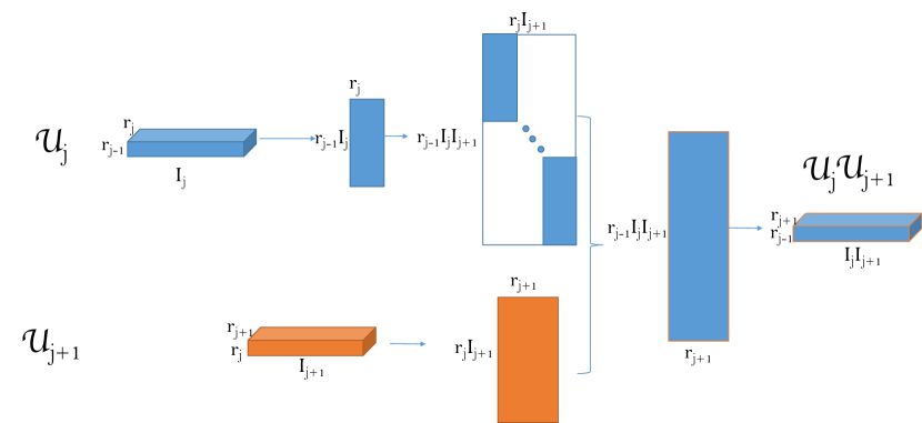
Figure 1: Tensor Connect Product for the $\mathscr{U}_{j}$ and $\mathscr{U}_{j+1}$. For tensor connect product with more than $2$ tensors, connect product the first two tensors and take the connect product tensor to connect product with the third tensor.

We first introduce three commonly used tensor unfolding operations namely, Tensor Mode-k Unfolding, Tensor Mode Matricization (TMM), Left-unfolding, and Right-unfolding as they will be intensively used in this paper.

Definition 1.

(Tensor Mode-k Unfolding)
The mode-$k$ unfolding matrix of a $n^{\text{th}}$ order tensor $\mathscr{X}\in\mathbb{R}^{I_{1}\times\cdots\times I_{n}}$, denoted as ${\bf X}_{[k]}\in\mathbb{R}^{I_{k}\times(I_{k+1}\cdots I_{n}I_{1}\cdots I_{k-1})}$, such that

$$\begin{split}&\mathscr{X}(i_{1},i_{2},\cdots,i_{n})\\ =&{\bf X}_{[k]}(i_{k},i_{k+1}+(i_{k+2}-1)I_{k+1}+\cdots\\ +&(i_{k-1}-1)\prod_{t=k+1,\cdots,n,1,\cdots k-1}I_{t}).\end{split}$$ (1)

Definition 2.

(Tensor Mode Matricization (TMM))
Let $\mathscr{X}\in\mathbb{R}^{I_{1}\times\cdots\times I_{n}}$ be a $n^{\text{th}}$ order tensor, the tensor mode matrization along the $k^{\text{th}}$ mode, denoted as $\mathscr{X}_{\lfloor k\rfloor}\in\mathbb{R}^{(\prod_{t=1}^{k}I_{t})\times(\prod_{t=k+1}^{n}I_{t})}$, is a matrix where

$$\begin{split}&\mathscr{X}(i_{1},\cdots,i_{n})\\ =&\mathscr{X}_{\lfloor i\rfloor}(i_{1}+(i_{2}-1)I_{1}+\cdots+(i_{k}-1)\prod_{t=1}^{k-1}I_{t},\\ &i_{k+1}+(i_{k+2}-1)I_{k+1}+\cdots+(i_{n}-1)\prod_{t=k+1}^{n-1}I_{t}).\end{split}$$ (2)

Definition 3.

(Left-unfolding & Right-unfolding [9])
Let $\mathscr{U}\in\mathbb{R}^{r_{0}\times I_{1}\times r_{1}}$ be a 3rd-order tensor, the left-unfolding of $\mathscr{U}$, denoted as ${\bf L}(\mathscr{U})$, satisfies the following property

$${\bf L}(\mathscr{U})\in\mathbb{R}^{(r_{0}I_{1})\times r_{1}},$$ (3)

and

$$\begin{split}{\bf L}(\mathscr{U})(k_{0}+(i_{1}-1)r_{0},k_{1})=\mathscr{U}(k_{0},i_{1},k_{1})\\ \forall k_{0}\in[1,r_{0}],k_{1}\in[1,r_{1}],i_{1}\in[1,I_{1}].\end{split}$$ (4)

And let ${\bf L}^{-1}$ be the reverse operation of ${\bf L}$, which reshapes a $\mathbb{R}^{(r_{0}I_{1})\times r_{1}}$ matrix to a $\mathbb{R}^{r_{0}\times I_{1}\times r_{1}}$ tensor.

Similarly, the right unfolding of $\mathscr{U}$, denoted as ${\bf R}(\mathscr{U})$, satisfies the following property

$${\bf R}(\mathscr{U})\in\mathbb{R}^{r_{0}\times(I_{1}r_{1})},$$ (5)

and

$$\begin{split}{\bf R}(\mathscr{U})(k_{0},i_{1}+(k_{1}-1)I_{1})=\mathscr{U}(k_{0},i_{1},k_{1})\\ \forall k_{0}\in[1,r_{0}],k_{1}\in[1,r_{1}],i_{1}\in[1,I_{1}],\end{split}$$ (6)

and ${\bf R}^{-1}$ is the reverse operation of ${\bf R}$, which reshapes a $\mathbb{R}^{r_{0}\times(I_{1}r_{1})}$ matrix to a $\mathbb{R}^{r_{0}\times I_{1}\times r_{1}}$ tensor.

Tensor train decomposition [4, 9] is a tensor factorization method that any elements inside a tensor $\mathscr{X}\in\mathbb{R}^{I_{1}\times\cdots\times I_{n}}$, denoted as $\mathscr{X}(i_{1},i_{2},\cdots,i_{n})$, is represented by

$$\mathscr{X}(i_{1},\cdots,i_{n})$$

$$={\bf U}_{1}(i_{1},:)\mathscr{U}_{2}(:,i_{2},:)\cdots\mathscr{U}_{n-1}(:,i_{n-1},:){\bf U}_{n}(:,i_{n}),$$ (7)

where ${\bf U}_{1}\in\mathbb{R}^{I_{1}\times r_{1}}$, ${\bf U}_{n}\in\mathbb{R}^{r_{n-1}\times I_{n}}$ are the boundary matrices and $\mathscr{U}_{i}\in\mathbb{R}^{r_{i-1}\times I_{i}\times r_{i}},i=2,\cdots,n-1$ are middle decomposed tensors.

A more general format of tensor train decomposition regards ${\bf U}_{1}\in\mathbb{R}^{I_{1}\times r_{1}}$ as a tensor $\mathscr{U}_{1}\in\mathbb{R}^{r_{0}\times I_{1}\times r_{1}},r_{0}=1$ and ${\bf U}_{n}\in\mathbb{R}^{r_{n-1}\times I_{n}}$ as a tensor $\mathscr{U}_{n}\in\mathbb{R}^{r_{n-1}\times I_{n}\times r_{n}},r_{n}=1$, which gives the general tenor train decomposition format

$$\mathscr{X}(i_{1},\cdots,i_{n})=\mathscr{U}_{1}(:,i_{1},:)\cdots\mathscr{U}_{n-1}(:,i_{n-1},:)\mathscr{U}_{n}(:,i_{n},:),$$ (8)

where $\mathscr{U}_{i}\in\mathbb{R}^{r_{i-1}\times I_{i}\times r_{i}},i=1,\cdots,n$ and $r_{0}=r_{n}=1$. The set of scalars, $[r_{0},r_{1},\cdots,r_{n-1},r_{n}]$, is defined as the tensor train rank (TT-Rank).

Since $\mathscr{X}(i_{1},\cdots,i_{n})$ is a scalar, (8) is equivalent to

$$\begin{split}\mathscr{X}(i_{1},\cdots,i_{n})=\text{Trace}(&\mathscr{U}_{1}(:,i_{1},:)\mathscr{U}_{2}(:,i_{2},:)\cdots\\ &\mathscr{U}_{n-1}(:,i_{n-1},:)\mathscr{U}_{n}(:,i_{n},:)),\end{split}$$ (9)

which enables the cyclic permutations property (See Definition 5 below) that is used intensively in this paper. Before defining this property, we define Tensor Connect Product, that describes the product of a sequence of $3$rd-order tensor.

Definition 4.

(Tensor Connect Product) Let $\mathscr{U}_{i}\in\mathbb{R}^{r_{i-1}\times I_{i}\times r_{i}},i=1,\cdots,n$ be $n$ $3$rd-order tensor, the tensor connect product is defined as,

$$\mathscr{U}=\mathscr{U}_{1}\cdots\mathscr{U}_{n}\in\mathbb{R}^{r_{0}\times(I_{1}\cdots I_{n})\times r_{n}}.$$ (10)

and is shown in Fig 1, where the tensor $\mathscr{U}_{j}$ is left-unfolded, denoted as ${\bf L}(\mathscr{U}_{j})$ and the tensor $\mathscr{U}_{j+1}$ is left-unfolded, denoted as ${\bf L}(\mathscr{U}_{j+1})$. Then

$$\begin{split}\mathscr{U}_{j}\mathscr{U}_{j+1}&\in\mathbb{R}^{r_{j-1}\times(I_{j}I_{j+1})\times r_{j+1}}\\ &={\bf L}^{-1}({\bf I}^{(I_{j+1})}\otimes{\bf L}(\mathscr{U}_{j})\times{\bf L}(\mathscr{U}_{j+1}))\end{split}$$ (11)

Let $f$ be a function applied on $\mathscr{U}$ such that $\mathscr{X}=f(\mathscr{U})\in\mathbb{R}^{I_{1}\times\cdots\times I_{n}}$ satisfies (9), then $f$ is the function that reshapes vector $(I_{1}\cdots I_{n})\times 1$ to tensor $I_{1}\times I_{2}\times\cdots\times I_{n}$ after applied trace operation on each slice the $\mathscr{U}$ along mode-$2$, denoted as

$$\mathscr{X}=f(\mathscr{U}),$$ (12)

or equivalently

$$\mathscr{X}=f(\mathscr{U}_{1}\cdots\mathscr{U}_{n}).$$ (13)

Tensor connect product gives the product rule for the production between $3^{\text{rd}}$-order tensor, just like the matrix product as for $2^{\text{nd}}$ order tensor. We further note that tensor connect product is the same as matrix product for $2^{\text{nd}}$-order tensor.

Lemma 1.

(Matrix Product) Tensor connect product is applied to matrix product. Let $M_{1}\in\mathbb{R}^{I_{1}\times r_{1}}$ and ${\bf M}_{2}\in\mathbb{R}^{r_{1}\times I_{2}}$ be any two matrix. Without loss of generality, we regard that ${\bf M}_{1}$ as a tensor $\mathscr{M}_{1}\in\mathbb{R}^{1\times I_{1}\times r_{1}}$ and ${\bf M}_{2}$ as $\mathscr{M}_{2}\in\mathbb{R}^{r_{1}\times I_{2}\times 1}$ , then tensor connect product gives the vectorized solution of matrix production

$$\mathscr{M}_{1}\mathscr{M}_{2}\in\mathbb{R}^{1\times(I_{1}I_{2})\times 1}=\text{vec}({\bf M}_{1}{\bf M}_{2}).$$ (14)

Proof.

Proof is in Appendix IX-A. ∎

Similar to matrix transpose, which can be regarded as an operation that cyclic swaps the two modes for a $2^{\text{nd}}$ order tensor, we defined Tensor Permutation to describe the cyclic-wise swap of tensor mode for high order tensor.

Definition 5.

(Tensor Permutation) For any order-$d$ tensor $\mathscr{X}\in\mathbb{R}^{I_{1}\times\cdots\times I_{d}}$, the $i^{\text{th}}$ tensor train permutation is defined as $\mathscr{X}^{P_{i}}\in\mathbb{R}^{I_{i}\times I_{i+1}\times\cdots\times I_{n}\times I_{1}\times I_{2}\times\cdots\times I_{i-1}}$ such that

$$\mathscr{X}^{P_{i}}(j_{i},\cdots,j_{n},j_{1},\cdots,j_{i-1})=\mathscr{X}(j_{1},\cdots,j_{n}),\forall_{i},j_{i}\in[1,I_{i}].$$ (15)

We note the following result.

Lemma 2.

$\mathscr{X}^{P_{i}}=f(\mathscr{U}_{i}\mathscr{U}_{i+1}\cdots\mathscr{U}_{n}\mathscr{U}_{1}\cdots\mathscr{U}_{i-1})$.

Proof.

Proof is in Appendix IX-B ∎

With this background and basic constructs we now outline the main problem set-up.

III Problem Setup

Given a tensor $\mathscr{X}\in\mathbb{R}^{I_{1}\times\cdots\times I_{n}}$ that is partially observed at locations $\Omega$, let $\mathscr{P}_{\Omega}\in\mathbb{R}^{I_{1}\times\cdots\times I_{n}}$ be the corresponding binary tensor in which $1$ represents an observed entry and $0$ represents a missing entry. The problem is to find a low tensor train rank (TT-Rank) approximation of the tensor $\mathscr{X}$, denoted as $\mathscr{W}$, such that the recovered tensor $\mathscr{W}$ matches $\mathscr{X}$ at $\mathscr{P}_{\Omega}$. This problem is referred as the tensor completion problem under tensor train model, which is equivalent to the following problem

$$\min_{\mathscr{W}:\mathscr{W}\text{ satisfies TT-Rank }{\bf r}}\|\mathscr{P}_{\Omega}\circ(\mathscr{W}-\mathscr{X})\|_{F}^{2}.$$ (16)

Using the factored form of TT representation, i.e. using equation (8), the above optimization problem is equivalent to solving the following problem,

$$\min_{\mathscr{U}_{i:i=1,2,\cdots,n}}\|\mathscr{P}_{\Omega}\circ(f(\mathscr{U}_{1}\mathscr{U}_{2}\cdots\mathscr{U}_{n}))-\mathscr{X}_{\Omega})\|_{F}^{2},$$ (17)

where the constraint that $\mathscr{W}$ is a low TT rank tensor is captured via $\mathscr{W}=\mathscr{U_{1}}\cdots\mathscr{U}_{n}$.

To solve this problem, We propose an algorithm referred to as Tensor Completion Algorithm by Alternating Minimization under the Tensor Train model, for short TCAM-TT, that solves the completion problem in two steps,

• Choosing an initial starting point by using Tensor Train Approximation (TTA) using the missing data only. This initialization algorithm is detailed in section IV.

• Updating the solution by applying Hierarchical Alternating Least Square (HALS) that alternatively (in a cyclic order) estimates a factor say $\mathscr{U}_{i}$ keeping the other factors fixed. This algorithm is detailed in Section V.

IV Tensor Train Approximation (TTA)

For a given tensor $\mathscr{X}$, we wish to find the tensor $\mathscr{W}$ of TT-rank ${\bf r}$ that best approximates $\mathscr{X}$. Thus, we want to solve the problem given by

$$\min_{\mathscr{W}:\mathscr{W}\text{ satisfies TT-Rank }{\bf r}}\|(\mathscr{W}-\mathscr{X})\|_{F}^{2}.$$ (18)

Rather than solving the problem (18) exactly, we give a heuristic algorithm to solve this problem. This is used as an initialization for the tensor completion problem, where the best approximation of zero-filled tensor will be used as an initialization. To avoid the computation complexity of (18), Algorithm 1 is used for the approximation. This algorithm gives the decomposition terms $\mathscr{U}_{i}$ of the approximate solution $\mathscr{W}$.

Algorithm 1 Tensor Train Approximation

1:Tensor $\mathscr{X}\in\mathbb{R}^{I_{1}\times I_{2}\times\cdots\times I_{n}}$, TT-rank $r_{i:i=1,2,\cdots,n-1}$, $r_{0}=r_{n}=1$

2:Tensor train decomposition $\mathscr{U}_{i}\in\mathbb{R}^{r_{i-1}\times I_{i}\times r_{i}},{i:i=1,2,\cdots,n}$

3:Tensor Unfolding: Apply tensor mode matrization for $\mathscr{X}$ along mode $1$ to get matrix ${\bf X}_{1}=\mathscr{X}_{\lfloor 1\rfloor}\in\mathbb{R}^{I_{1}\times(I_{2}I_{3}\cdots I_{n})}$

4:Apply SVD and threshold the number of singular values to be $r_{1}$ such that ${\bf X}_{1}={\bf U}_{1}{\bf S}_{1}{\bf V}_{1}^{\top},{\bf U}_{1}\in\mathbb{R}^{I_{1}\times r_{1}},{\bf S}_{1}\in\mathbb{R}^{r_{1}\times r_{1}},{\bf V}_{1}\in\mathbb{R}^{r_{1}\times(I_{2}I_{3}\cdots I_{n})}$. Note that ${\bf U}_{1}={\bf L}(\mathscr{U}_{1})$, thus reshape ${\bf U}_{1}$ to $\mathbb{R}^{r_{0}\times I_{1}\times r_{1}}$ to recover $\mathscr{U}_{1}$ and let ${\bf M}_{1}={\bf S}_{1}{\bf V}_{1}^{\top}\in\mathbb{R}^{r_{1}\times({I_{2}I_{3}\cdots I_{n}})}$

5:for  $i=2$ to $n-1$ do

6:   Reshape ${\bf M}_{i-1}\in\mathbb{R}^{r_{i-1}\times(I_{i}I_{i+1}\cdots I_{n})}$ to ${\bf X}_{i}\in\mathbb{R}^{(r_{i-1}I_{i})\times(I_{i+1}I_{i+2}\cdots I_{n})}$

7:   Compute SVD and threshold the number of singular values to be $r_{i}$ such that ${\bf X}_{i}={\bf U}_{i}{\bf S}_{i}{\bf V}_{i}^{\top},{\bf U}_{i}\in\mathbb{R}^{(r_{i-1}I_{i})\times r_{i}},{\bf S}_{i}\in\mathbb{R}^{r_{i}\times r_{i}},{\bf V}\in\mathbb{R}^{r_{i}\times(I_{i+1}I_{i+2}\cdots I_{n})}$. Note that ${\bf U}_{i}={\bf L}(\mathscr{U}_{i})$, thus reshape ${\bf U}_{i}\in\mathbb{R}^{(r_{i-1}I_{i})\times r_{i}}$ to $\mathbb{R}^{r_{i-1}\times I_{i}\times r_{i}}$ to get $\mathscr{U}_{i}$ and set ${\bf M}_{i}={\bf S}_{i}{\bf V}_{i}^{\top}\in\mathbb{R}^{r_{i}\times(I_{i+1}I_{i+2}\cdots I_{n})}$

8:end for

9:Reshape ${\bf M}_{n-1}\in\mathbb{R}^{r_{n-1}\times I_{n}}$ to $\mathbb{R}^{r_{n-1}\times I_{n}\times r_{n}}$ to get $\mathscr{U}_{n}$

10:Return $\mathscr{U}_{1},\cdots,\mathscr{U}_{n}$

The proposed algorithm is a modified version of the tensor train decomposition as proposed in [10]. In the tensor train decomposition algorithm of [10], the tensor is exactly TT-Rank ${\bf r}$. However, in our problem, the tensor $\mathscr{X}$ is not necessarily a TT-Rank ${\bf r}$ tensor. Thus, the singular value decomposition (SVD) is performed in different modes and thresholded to obtain the approximate TT-Rank ${\bf r}$ tensor.

V Hierarchical Alternating Least Square (HALS)

The proposed Tensor Completion method by Alternating Minimization under Tensor Train model (TCAM-TT) solves (17) by taking orders to solve the following problem

$$\mathscr{U}_{i}={\text{argmin}}_{\mathscr{Y}}\|\mathscr{P}_{\Omega}\circ f(\mathscr{U}_{1}\cdots\mathscr{U}_{i-1}\mathscr{Y}\mathscr{U}_{i+1}\cdots\mathscr{U}_{n})-\mathscr{X}_{\Omega})\|_{F}^{2}$$ (19)

We further note that $\mathscr{U}_{i}$ in (19) can be solved only considering the following optimization problem

$$\mathscr{U}_{1}={\text{argmin}}_{\mathscr{Y}\in\mathbb{R}^{r_{0}\times I_{1}\times r_{1}}}\|\mathscr{P}_{\Omega}\circ f(\mathscr{Y}\mathscr{U}_{2}\cdots\mathscr{U}_{n})-\mathscr{X}_{\Omega})\|_{F}^{2}.$$ (20)

Lemma 3.

When $i\neq 1$, solving

$$\mathscr{U}_{i}={\text{argmin}}_{\mathscr{Y}}\|\mathscr{P}_{\Omega}\circ f(\mathscr{U}_{1}\cdots\mathscr{U}_{i-1}\mathscr{Y}\mathscr{U}_{i+1}\cdots\mathscr{U}_{n})-\mathscr{X}_{\Omega})\|_{F}^{2}$$ (21)

is equivalent to

$$\mathscr{U}_{i}={\text{argmin}}_{\mathscr{Y}}\|\mathscr{P}^{P_{i}}_{\Omega}\circ f(\mathscr{Y}\mathscr{U}_{i+1}\cdots\mathscr{U}_{n}\mathscr{U}_{1}\cdots\mathscr{U}_{i-1})-\mathscr{X}^{P_{i}}_{\Omega}\|_{F}^{2}.$$ (22)

Since the format of (22) is exactly the same as (20), thus solving $\mathscr{U}_{i}$ is equivalent to solving $\mathscr{U}_{1}$.

Proof.

Proof is in Appendix IX-C ∎

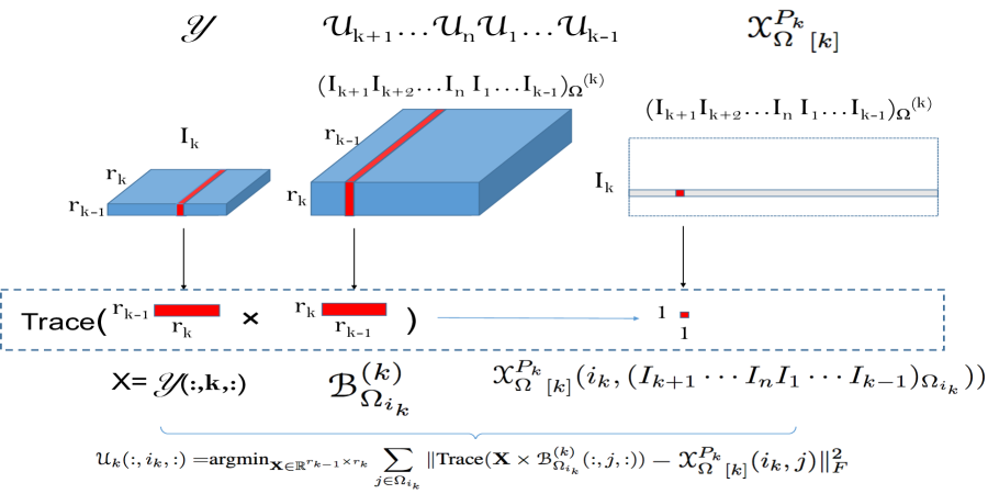
Figure 2: Updating $\mathscr{U}_{k}$ by Hierarchical Alternating Least Square (HALS)

Now we consider solving $\mathscr{U}_{k}$ without loss of generality. Based on Lemma 3, we need to solve the following problem

$$\mathscr{U}_{k}={\text{argmin}}_{\mathscr{Y}}\|\mathscr{P}^{P_{k}}_{\Omega}\circ f(\mathscr{Y}\mathscr{U}_{k+1}\cdots\mathscr{U}_{n}\mathscr{U}_{1}\cdots\mathscr{U}_{k-1})-\mathscr{X}^{P_{k}}_{\Omega}\|_{F}^{2}.$$ (23)

We further apply tensor mode-$k$ unfolding, which gives the equivalent problem

$$\mathscr{U}_{k}={\text{argmin}}_{\mathscr{Y}}\|{\mathscr{P}^{P_{k}}_{\Omega}}_{[k]}\circ{f(\mathscr{Y}\mathscr{U}_{k+1}\cdots\mathscr{U}_{n}\mathscr{U}_{1}\cdots\mathscr{U}_{k-1})}_{[k]}-{\mathscr{X}^{P_{k}}_{\Omega}}_{[k]}\|_{F}^{2}.$$ (24)

where ${\mathscr{P}^{P_{k}}_{\Omega}}_{[k]}$, ${f(\mathscr{Y}\mathscr{U}_{k+1}\cdots\mathscr{U}_{n}\mathscr{U}_{1}\cdots\mathscr{U}_{k-1})}_{[k]}$ and ${\mathscr{X}^{P_{k}}_{\Omega}}_{[k]}$ are matrices with dimension $\mathbb{R}^{I_{k}\times(I_{k+1}\cdots I_{n}I_{1}\cdots I_{k-1})}$.

The trick in solving (24) is that each slice of tensor $\mathscr{Y}$, denoted as $\mathscr{Y}(:,i_{k},:),i_{k}=1,\cdots,I_{k}$ which corresponds to each row of ${\mathscr{P}^{P_{k}}_{\Omega}}_{[k]}$, ${f(\mathscr{Y}\mathscr{U}_{k+1}\cdots\mathscr{U}_{n}\mathscr{U}_{1}\cdots\mathscr{U}_{k-1})}_{[k]}$ and ${\mathscr{X}^{P_{k}}_{\Omega}}_{[k]}$, can be solved independently, thus equation (20) can be solved by solving $I_{k}$ equivalent subproblems

$$\begin{split}&\mathscr{U}_{k}(:,i_{k},:)\\ =&{\text{argmin}}_{{\bf X}\in\mathbb{R}^{r_{k-1}\times 1\times r_{k}}}\|{\mathscr{P}^{P_{k}}_{\Omega}}_{[k]}(i_{k},:)\circ f({\bf X}\mathscr{U}_{k+1}\cdots\mathscr{U}_{k-1})\\ &-{\mathscr{X}^{P_{k}}_{\Omega}}_{[k]}(i_{k},:)\|_{F}^{2}\end{split}$$ (25)

As shown in Fig 2.

Let $\mathscr{B}^{(k)}=\mathscr{U}_{k+1}\cdots\mathscr{U}_{n}\mathscr{U}_{1}\cdots\mathscr{U}_{k-1}\in\mathbb{R}^{r_{k}\times(I_{k+1}\cdots I_{n}I_{1}\cdots I_{k-1})\times r_{k-1}}$. Let $\mathscr{B}^{(k)}_{\Omega_{i_{k}}}\in\mathbb{R}^{r_{k}\times(I_{k+1}\cdots I_{n}I_{1}\cdots I_{k-1})_{\Omega_{i_{k}}}\times r_{k-1}}$ be the components in $\mathscr{B}^{(k)}$ such that ${\mathscr{P}^{P_{k}}_{\Omega}}_{[k]}(i_{k},(I_{k+1}\cdots I_{n}I_{1}\cdots I_{k-1})_{\Omega_{i_{k}}})$ are observed.

Thus equation (25) is equivalent to

$$\begin{split}\mathscr{U}_{k}(:,i_{k},:)=&{\text{argmin}}_{\mathscr{Z}}\|f(\mathscr{Z}\mathscr{B}^{(k)}_{\Omega_{i_{k}}})\\ &-{\mathscr{X}^{P_{k}}_{\Omega}}_{[k]}(i_{k},(I_{k+1}\cdots I_{n}I_{1}\cdots I_{k-1})_{\Omega_{i_{k}}}))\|_{F}^{2}\end{split}$$ (26)

where $\mathscr{Z}\in\mathbb{R}^{r_{k-1}\times 1\times r_{k}}$, $\mathscr{B}^{(k)}_{\Omega_{i_{k}}}\in\mathbb{R}^{r_{k}\times(I_{k+1}\cdots I_{k-1})_{\Omega_{i_{k}}}\times r_{k-1}}$, ${\mathscr{X}^{P_{k}}_{\Omega}}_{[k]}(i_{k},(I_{k+1}\cdots I_{n}I_{1}\cdots I_{k-1})_{\Omega_{i_{k}}}))\in\mathbb{R}^{1\times(I_{k+1}\cdots I_{k-1})_{\Omega_{i_{k}}}}$

We regard $\mathscr{Z}\in\mathbb{R}^{r_{k-1}\times 1\times r_{k}}$ as a matrix ${\bf X}\in\mathbb{R}^{r_{k-1}\times r_{k}}$. Since the Frobenius norm of a vector in (26) is equivalent to entry-wise square summation of all entries, we rewrite (26) as

$$\begin{split}\mathscr{U}_{k}(:,i_{k},:)=&{\text{argmin}}_{{\bf X}\in\mathbb{R}^{r_{k-1}\times r_{k}}}\sum_{j\in\Omega_{i_{k}}}\|\text{Trace}({\bf X}\times\mathscr{B}^{(k)}_{\Omega_{i_{k}}}(:,j,:))\\ &-{\mathscr{X}^{P_{k}}_{\Omega}}_{[k]}(i_{k},j)\|_{F}^{2}\end{split}$$ (27)

where $\times$ is the matrix product.

Lemma 4.

Let ${\bf A}\in\mathbb{R}^{r_{1}\times r_{2}}$ and ${\bf B}\in\mathbb{R}^{r_{2}\times r_{1}}$ be any two matrices, then

$$\begin{split}\text{Trace}({\bf A}\times{\bf B})&=vec({\bf A})^{\top}vec({\bf B}^{\top})=vec({\bf B}^{\top})^{\top}vec({\bf A})\end{split}$$ (28)

Proof.

Proof is in Appdendix IX-D. ∎

Based on Lemma 4, (27) becomes

$$\begin{split}\mathscr{U}_{k}(:,i_{k},:)={\text{argmin}}_{\bf X}\sum_{j\in\Omega^{(k)}_{i_{k}}}\|&vec((\mathscr{B}^{(k)}_{\Omega_{i_{k}}}(:,j,:))^{\top})^{\top}vec({\bf X})\\ &-{\mathscr{X}^{P_{k}}_{\Omega}}_{[k]}(i_{k},j)\|_{F}^{2}\end{split}$$ (29)

Then the problem for solving $\mathscr{U}_{k}[:,i_{k},:]$ becomes a least square problem. Solving $I_{k}$ least square problem would give the optimal solution for $\mathscr{U}_{k}$. Since each $\mathscr{U}_{i:i=1,\cdots,n}$ can solved by a least square method, tensor completion under tensor train model can be solved by taking orders to update $U_{i:i=1,\cdots,n}$ until convergence.

Algorithm 2 TCAM-TT Algorithm

1:Zero-filled Tensor $\mathscr{X}_{\Omega}\in\mathbb{R}^{I_{1}\times I_{2}\times...\times I_{n}}$, binary observation index tensor $\mathscr{P}_{\Omega}\in\mathbb{R}^{I_{1}\times I_{2}\times...\times I_{n}}$, TT-rank $r_{i:i=1,2,...,n-1}$, thresholding parameter $tot$, maximum iteration $maxiter$

2:Recovered tensor $\mathscr{X}_{R}$

3:Tensor Train Decomposition Approximation Apply tensor train decomposition approximation in Algorithm 1 on $\mathscr{X}_{\Omega}$ to initialize the decomposition terms $\mathscr{U}_{i:i=1,...,n}^{(0)}$. Set iteration parameter $\ell=0$.

4:while  $\ell\leq maxiter$  do

5:   $\ell=\ell+1$

6:   for $i=1$ to $n$ do

7:      Solve by Least Square Method ${\mathscr{U}_{i}}^{(\ell)}={\text{argmin}}_{\mathscr{U}}\|\mathscr{P}_{\Omega}\circ(\mathscr{U}\mathscr{U}_{i+1}^{(\ell-1)}...\mathscr{U}_{n}^{(\ell-1)}\mathscr{U}_{1}^{(\ell)}...\mathscr{U}_{i-1}^{(\ell)}-\mathscr{X})\|_{F}^{2}$

8:   end for

9:   if $\sum_{i}\frac{\|\mathscr{U}_{i}^{(\ell+1)}-\mathscr{U}_{i}^{(\ell)}\|_{F}}{\|{\mathscr{U}}^{(\ell)}_{i}\|_{F}}\leq tot$ then

10:      Break

11:   end if

12:end while

13:Recover Completed Tensors $\mathscr{X}_{R}=\mathscr{U}_{1}^{(\ell)}\mathscr{U}_{2}^{(\ell)}...\mathscr{U}_{n-1}^{(\ell)}\mathscr{U}_{n}^{(\ell)}$

The convergence criterion for the proposed TCAM-TT algorithm is defined via a threshold on the relative change, say $\epsilon$, in the successive estimation of the factors,

$$\epsilon=\sum_{i}\frac{\|\mathscr{U}_{i}^{(\ell+1)}-\mathscr{U}_{i}^{(\ell)}\|_{F}}{\|{\mathscr{U}}^{(\ell)}_{i}\|_{F}}$$ (30)

where $\ell$ is the iteration parameter and $maxiter$ is maximum iterations. The algorithm will stops either when $\ell$ reaches $maxiter$ or when the relative error $\epsilon\leq tot$ for some predefined tolerance parameter $tot$.

VI Complexity Analysis

The main algorithm in the computation is the computation of the least squares. This computation is performed for each slice of each tensor train factors $\mathscr{U}_{k=1,\cdots,n}(:,i_{k},:),i_{k}\in 1,\cdots I_{k}$. The matrix corresponding to the least square problem $(\|{\bf A}x-{\bf b}\|_{F})$ satisfies ${\bf A}\in\mathbb{R}^{P_{k,i_{k}}\times(r_{k-1}r_{k})}$, where $P_{k,i_{k}}$ is the number of observed entries in the $i_{k}^{\text{th}}$ in $\mathscr{X}_{[k]}$. For the analysis, we assume that all ranks are the same, or $r_{k}=r$. Since the complexity of pseudo-inverse of $d_{1}\times d_{2}$ matrix is $O(d_{1}^{2}d_{2})$ [11], this complexity is given as $O(P_{k,i_{k}}r^{2}_{k-1}r^{2}_{k})$. Thus, the overall complexity in each iteration is given as $O(nPr^{4})$, where $P$ is the total number of observed entries.

VII Numerical Results

In this section, we compare our proposed TCAM-TT algorithm with Tensor Completion by alternating Minimization after Tensor Mode Matrization (TCAM-TMM), SiLRTC-TT algorithm as proposed in [8] and tSVD algorithm as proposed in [12]. We briefly describe these algorithms below.

VII-A TCAM-TMM

The first tensor completion algorithm is TCAM-TMM algorithm where a tensor is unfolded into matrix and alternating minimization [6] is used to solve the resulting matrix completion problem. For an order-$n$ tensor with a given set of tensor train rank, TCAM-TMM algorithm uses the $n-1$ possible ways of of tensor mode matricization ( see section II, Definition 2.

In particular, let $\mathscr{X}_{\lfloor k:k=1,\cdots,n-1\rfloor}\in\mathbb{R}^{(\prod_{t=1}^{k}I_{t})\times(\prod_{t=k+1}^{N}I_{t})}$ be the tensor the $k^{\text{th}}$ mode matrization of tensor $\mathscr{X}\in\mathbb{R}^{I_{1}\times...\times I_{n}}$, thus TCAM-TMM solves the tensor completion problem by solving the following matrix completion problem,

$$\min_{{\bf U}_{k},{\bf V}_{k}}\|\mathscr{P}_{\Omega_{\lfloor k\rfloor}}\circ({\bf U}_{k}{\bf V}_{k}^{\top}-\mathscr{X}_{\lfloor k\rfloor})\|_{F},$$ (31)

where $\mathscr{P}_{\Omega_{\lfloor k\rfloor}}$ is the binary tensor after the $k^{\text{th}}$ tensor mode matrization, ${\bf U}_{k}$ and ${\bf V}_{k}$ are the low-rank factorization terms of the tensor $\mathscr{X}$ after the $k^{\text{th}}$ tensor mode matrization and the rank is the $r_{k}$, which is selected from the tensor train rank.

VII-B SiLRTC-TT

The second tensor completion algorithm is SiLRTC-TT algorithm as proposed in [8], which completes tensors by taking orders to do matrix completion after tensor mode unfolding and recovery the tensor by weighted summarization of the tensor after each matrix completion. It is selected as it has been shown to have the best performance in [8].

VII-C tSVD

The third tensor completion algorithm is the tubal-SVD (t-SVD) based algorithm as proposed in [12, 13]. This algorithm works by minimizing the nuclear norm of a block circulant matrix that is formed out of the slices of the tensor. This algorithm is selected as it shows very good performance for video completion.

The performance of all these algorithms are measured by the Recovery Error at Missing Entries (REME), defined as

$$\text{REME}=\frac{\|\mathscr{X}_{-\Omega}-\mathscr{X}^{(R)}_{-\Omega}\|_{F}}{\|\mathscr{X}_{-\Omega}\|_{F}},$$ (32)

where $\mathscr{X}_{-\Omega}$ represents missing entries in the original tensor, $\mathscr{X}^{(R)}_{-\Omega}$ represents missing entries in the recovered tensor.

VII-D Synthetic Data

In this section, we consider a completion problem of a $4$ dimensional tensor $\mathscr{X}\in\mathbb{R}^{20\times 20\times 20\times 20}$ with TT-Rank $[1,5,100,5,1]$ without loss of generality. The tensor is generated by a sequence of connected tensors $\mathscr{U}_{i:i=1,2,3,4}$, and all the entries in $\mathscr{U}_{i}$ are sampled from independent standard normal distribution.

The 4-D tensor $\mathscr{X}$ with a pre-defined tensor train rank has $3$ tensor mode matrization, and each tensor mode matrixzation, denoted as $\mathscr{X}_{\lfloor k\rfloor,k=1,2,3}$ generates a matrix completion problem of $\mathscr{X}_{\lfloor 1\rfloor}\in\mathbb{R}^{20\times 8000}$, $\mathscr{X}_{\lfloor 2\rfloor}\in\mathbb{R}^{400\times 400}$ and $\mathscr{X}_{\lfloor 3\rfloor}\in\mathbb{R}^{8000\times 20}$ with rank $5$, $100$ and $5$ respectively. The completion results after each tensor mode matrization (TMM) are denoted as TCAM-TMM1, TCAM-TMM2, and TCAM-TMM3.

The error tolerance $tot$ for all algorithm is set to be $10^{-4}$. Thus any REME that is lower than $10^{-4}$ is regarded as a perfect completion. The maximum iteration, $maxiter$, is set to be $100$ for TCAM-TT and $1000$ for TCAM-TMM1, TCAM-TMM2, TCAM-TMM3, SiLRTC-TT, and tSVD algorithm.

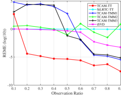
Figure 3: Tensor completion under tensor train model for synthetic tensor $\mathscr{X}\in\mathbb{R}^{20\times 20\times 20\times 20}$ with TT-rank $[1,5,100,5,1]$

The simulation in Fig 3 shows the REME at log10 scale for observation ratio from $10\%$ to $90\%$ of all algorithms and each plotted point is the average of 12 independent repeated experiment. TCAM-TT algorithm performs the best as it achieves perfectly tensor recovery for any observation ratio higher $20\%$ while TCAM-TMM1, TCAM-TMM3, and tSVD achieve perfectly recovery at the sampling ratio $70\%$, $70\%$, and $90\%$ . TCAM-TMM2 and SiLRTC-TT are not effective in tensor completion in this case as the recovery errors for the two algorithms are around $1$. TCAM-TT algorithm achieve the best performances as it consider all the tensor train rank together and the updating of each alternating minimization step maintains the TT-Rank property. In contrast, TACM-TMM, SiLRTC-TT and tSVD algorithm consider each tensor train rank independently, thus the completion results fit one specific rank of the TT-Rank very well but may not fit all the TT-Rank, which leads to the lower performance.

Figure 4: TCAM-TT algorithm convergence for synthetic tensor $\mathscr{X}\in\mathbb{R}^{20\times 20\times 20\times 20}$ with TT-rank $[1,5,100,5,1]$

In addition to better recovery as compared with the other algorithms, TCAM-TT algorithm converges within less number of alternating minimization iterations. The convergence performance of TCAM-TT algorithm for observation ratio from 12% to 50% is shown in Fig 4. We note that for any observation ratio larger than $15\%$ TCAM-TT takes less than $80$ iterations. Typically, the larger the observation ratio, the less iteration it takes for TCAM-TT to converge. For example, the tensor with $50\%$ observation ratio only takes $19$ iterations to converge with the REME being $10^{-16}$. This fast convergence is in part due to good initialization when more data is available.

VII-E Extended YaleFace Dataset B

Extended YaleFace Dataset B [14] is a dataset that includes 38 people with 9 poses under 64 illumination conditions. Each image has the size of $192\times 168$, where we down-sample the size of each image to $48\times 42$ for ease of calculation. We consider the images for 38 people under 64 illumination within 1 pose by reshaping the data into a tensor $\mathscr{X}\in\mathbb{R}^{48\times 42\times 64\times 38}$. TT-rank is estimated to be $[1,31,137,31,1]$, which gives $10\%$ error for fitting the dataset when there are no missing entries. Missing entries are sampled by assuming that data is entry-wise missing with probability $p$, where $p$ changes from $10\%$ to $90\%$. The error tolerance $tot$ for all algorithm is again set to be $10^{-4}$ and the maximum iteration $maxiter$ is set to be $20$ for TCAM-TT while the maximum iteration for TCAM-TMM1, TCAM-TMM2, TCAM-TMM3, SiLRTC-TT and tSVD are all set to be $1000$.

The simulation results shown in Fig 5 describe the completed images under $70\%$ and $80\%$ observation and the table in Fig 6 shows the REME values for each algorithm.

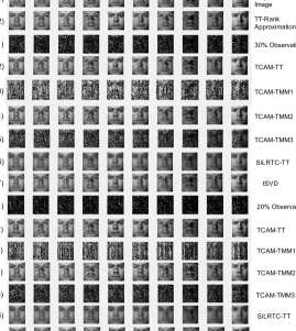
Figure 5: Tensor completion for Extended YaleFace Dataset B. (a1) Original 10 images selected from the dataset. (a2) 10 images after TT-rank $[1,31,137,31,1]$ approximation when no missing entries where the recovery error is $10\%$. (b1-b7) shows missing data, TCAM-TT completed data, TCAM-TMM1 completed data, TCAM-TMM2 completed data,TCAM-TMM3 completed data, SiLRTC-TT completed data and tSVD completed under the scenario when each entry is missing with probability $0.7$. (c1-c7) shows missing data, TCAM-TT completed data, TCAM-TMM1 completed data, TCAM-TMM2 completed data,TCAM-TMM3 completed data, SiLRTC-TT completed data and tSVD completed under the scenario when each entry is missing with probability $0.8$.

Figure 6: REME for Extended YaleFace Dataset B Completion at Observation Ratio $20\%$, $30\%$, $40\%$ and $50\%$

Noting that under $70\%$ observation ratio, only TCAM-TT, TCAM-TMM2, SiLRTC-TT and tSVD can complete the images while TCAM-TMM1 and TCAM-TMM3 algorithm can not, thus only TCAM-TT, TCAM-TMM2, SiLRTC-TT and tSVD algorithm are considered for investigating the relation between observation ratio and REME for Extended YaleFace Dataset B, as shown in Fig 7.

SiLRTC-TT and tSVD algorithm both show stable recovery result for all sampling ratios. When sampling ratio decreases from $60\%$ to $10\%$, the recovery error increases from $25.57\%$ and $12.3\%$ to $38.80\%$ and $26.7\%$, which shows the stable performance in all the algorithm. However, the stable performance comes with the cost of blurry recovery, as shown in Fig 5 (b6) and (b7), where although the recovery result is smooth, each image is less sharp in resolution. tSVD algorithm performs better than SiLRTC-TT algorithm under any observation ratio.

Both TCAM-TT and TCAM-TMM2 algorithm have shown good recovery when the sampling ratio is greater than $40\%$ and the increasing of error of recovery when the sampling ratio becomes lower. The recovery result for TCAM-TMM2 starts to degrade at $40\%$ sampling ratio and the error increases faster thanTCAM-TT algorithm, as TCAM-TMM2 does not capture the tensor structure in first and third unfolding of the tensor. TCAM-TT algorithm shows the best result for all sampling ratio larger than $20\%$.

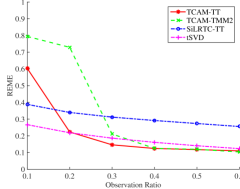
Figure 7: REME versus observation ratio from 10% to 60% for Extended YaleFace Dataset B

VII-F Video Data

The Video data we used is high speed camera video for bullet we downloaded from Youtube [15] with $85$ frames in total and each frame is consisted by a $100\times 260\times 3$ color image. The video data is regarded as a 4-mode tensor $\mathscr{X}\in\mathbb{R}^{100\times 260\times 3\times 85}$. Different from the tensor constructed from Extended YaleFace Dataset B where the $4^{\text{th}}$ mode of the tensor that represents different persons only has weak connections, the $4^{\text{th}}$ mode of the tensor built from the video data owns a stronger connection and the lower rank property is more likely to hold as the $4^{\text{th}}$ mode of the tensor represents the time series and any frame is easily to be represented by the linear combination of its previous frame and its next frame. The TT-rank is estimated to be $[1,29,99,19,1]$, which gives $6.33\%$ error for fitting the dataset when there are no missing data.

This video is selected as under high speed, gun and hand are almost still while smoke and bullet are movable, which could show the algorithm recovery performance on both still and dynamic objects within video. The $1^{\text{st}}$ frame of the recovered video image is shown in Fig 8, where entries in video are set to be missing independently with probability $p$, which changes from $10\%$ to $90\%$ at the step of $10\%$.

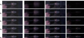
Figure 8: Video completion by TCAM-TT, SiLRTC, and tSVD under observation ratio $10\%$, $20\%$, $30\%$, $40\%$, and $50\%$. The $1^{st}$ frame of the video is displayed.

TCAM-TT, TCAM-TMM1, TCAM-TMM2, TCAM-TMM3, SiLRTC-TT and tSVD algorithm are implemented while only TCAM-TT, SiLRTC-TT and tSVD algorithm are able to complete the video when the observation ratio is less than $70\%$, showing the advantage of tensor completion as compared with matrix completion when high order data is considered. Completion result in Fig 8 shows that TCAM-TT algorithm out performs than SiLRTC-TT algorithm as the still objects can be recovered completely and dynamic objects can be recovered smoothly for adjacent frames. In contrast, SiLRTC-TT algorithm does not complete the video completely as the hand in the figure is blurred by the uncompleted dots.

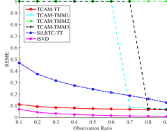
Figure 9: REME versus observation ratio from 10% to 90% for Video Completion

Figure 9 shows the REME for observation from $10\%$ to $90\%$, where any REME larger than $1$ is set to be $1$ for ease of visualization. The completion results for SiLRTC-TT degrades faster than TCAM-TT algorithm when the observation ratio decreases since the video becomes more uniformly dark and more blurry when the missing ratio increases from $50\%$ to $90\%$. In the video completion, tSVD performs the best of all the algorithm, which benefits from the advantage of Fourier transform that is applied on time series. The error in the proposed algorithm is limited by the error in TT-rank approximation of the actual data with the chosen rank. The proposed algorithm performs the best among the other algorithms, and in specific as compared to the other algorithms that exploit the TT-rank structures and the matrix unfolding based approaches.

VII-G Seismic Data

In thie subsection, we widh to complete pre-stack seismic records from incomplete spatial measurements. The pre-stack seismic data can be viewed as a 5D data or a fifth order tensor consisting of one time or frequency dimension and four spatial dimensions describing the location of the detector and the receiver in a two dimensional plane. This data can then be described in terms of the original $(r_{x},r_{y},s_{x},s_{y})$ coordinate frames or in terms of midpoint receivers and offsets $(x,y,h_{x},h_{y})$ [16]. We use the dataset from [16], where the sources and receivers are placed on a $16\times 16$ grid with $50m$ shot forming a tensor $\mathscr{X}\in\mathbb{R}^{16\times 16\times 17\times 17\times 150}$. We approximate the TT- Rank of this tensor as $[1,1,1,9,41,1]$.

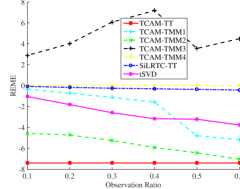
Figure 10: REME versus observation ratio from 10% to 60% for Seismic Data

The results in Figure 10 illustartes that the proposed algorithm performs significantly better than other compared algorithms for different observation ratios from 10% to 60%.

VIII Conclusion

We proposed a novel algorithm for data completion using tensor train decomposition. Unlike the current methods exploiting this format, our algorithm exploits the matrix product state representation and uses alternating minimization over the low rank factors for completion. As a future work we will derive provable performance guarantees on tensor completion using the proposed algorithm. In this context, the statistical machinery for proving analogous results for the matrix case [xx] can be used. We will also look at parallelizing this algorithm and make it more efficient in terms of implementation, especially when forming and storing the intermediate tensors from the estimated factors.

IX appendix

IX-A Proof of Lemma 1

Proof.

Let ${\bf M}={\bf M}_{1}{\bf M}_{2}$, thus

$${\bf M}(j_{1},j_{2})=\sum_{j=1}^{r_{1}}{\bf M}_{1}(j_{1},j){\bf M}_{2}(j,j_{2})$$ (33)

where ${\bf M}(j_{1},j_{2})$ locates at $\text{vec}({\bf M}_{1}{\bf M}_{2})(j_{1}+(j_{2}-1)I_{1},1)$.

Let ${\bf T}_{1}\in\mathbb{R}^{(I_{1}I_{2})\times(r_{1}I_{2})}={\bf I}^{(I_{2})}\otimes{\bf L}(\mathscr{M}_{1})$ and ${\bf T}_{2}\in\mathbb{R}^{(r_{1}I_{2})\times 1}={\bf L}(\mathscr{M}_{2})$, and ${\bf T}\in\mathbb{R}^{I_{1}I_{2}\times 1}={\bf T}_{1}{\bf T}_{2}$, thus

$$\begin{split}&{\bf T}(j_{1}+(j_{2}-1)I_{1},1)\\ =&\sum_{j=1}^{r_{1}I_{2}}{\bf T}_{1}(j_{1}+(j_{2}-1)I_{1},j){\bf T}_{2}(j,1)\\ =&\sum_{j=(j_{2}-1)r_{1}+1}^{j_{2}r_{1}}{\bf T}_{1}(j_{1}+(j_{2}-1)I_{1},j){\bf T}_{2}(j,1)\\ =&\sum_{j=1}^{r_{1}}{\bf M}(j_{1},j){\bf M}_{2}(j,j_{2})\end{split}$$ (34)

We conclude that any ${j_{1}+(j_{2}-1)I_{1}}^{\text{th}}$ entry on the left hand side is the same as that on the right hand side, thus we prove our claim. ∎

IX-B Proof of Lemma 2

Proof.

Based on definition of tensor permutation in (15), on the left hand side, the $(j_{1},....,j_{n})$ entry of the tensor is

$$\mathscr{X}^{P_{i}}(j_{1},...,j_{n})=\mathscr{X}(j_{n-i+2},...,j_{n},j_{1},...,j_{n-i+1}).$$ (35)

On the right hand side, the $(j_{1},....,j_{n})$ entry of the tensor gives

$$\begin{split}&f(\mathscr{U}_{i}\cdots\mathscr{U}_{i-1})(j_{1},\cdots,j_{n})\\ =&\text{Trace}(\mathscr{U}_{i}(:,j_{1},:)\mathscr{U}_{i+1}(:,j_{2},:)...\mathscr{U}_{n}(:,j_{n-i+1},:)\\ &\mathscr{U}_{1}(:,j_{n-i+2},:)\cdots\mathscr{U}_{i-1}(:,j_{n},1)).\end{split}$$ (36)

Since trace is invariant under cyclic permutations, we have

$$\begin{split}&\text{Trace}(\mathscr{U}_{i}(:,j_{1},:)\mathscr{U}_{i+1}(:,j_{2},:)...\mathscr{U}_{n}(:,j_{n-i+1},:)\\ &\mathscr{U}_{1}(:,j_{n-i+2},:)\cdots\mathscr{U}_{i-1}(:,j_{n},1))\\ =&\text{Trace}(\mathscr{U}_{1}(:,j_{n-i+2},:)\cdots\mathscr{U}_{i-1}(:,j_{n},1)\\ &\mathscr{U}_{i}(:,j_{1},:)\mathscr{U}_{i+1}(:,j_{2},:)...\mathscr{U}_{n}(:,j_{n-i+1},:))\\ =&f(\mathscr{U}_{1}\cdots\mathscr{U}_{n})(j_{n-i+2},\cdots,j_{n},j_{1},\cdots,j_{n-i+1}),\end{split}$$ (37)

which equals to the right hand side of equation (35) based on (13). Since any entries in $\mathscr{X}^{P_{i}}$ are the same as those in $\mathscr{U}_{i}\mathscr{U}_{i+1}\cdots\mathscr{U}_{n}\mathscr{U}_{1}\cdots\mathscr{U}_{i-1}$, the claim is proved. ∎

IX-C Proof of Lemma 3

Proof.

First we note that tensor permutation does not change tensor Frobenius norm as all the entries remain the same as those before the permutation. Thus, when $i\neq 1$, we permute the tensor inside the Frobenius norm in (21) and get the equivalent equation as

$$\mathscr{U}_{i}={\text{argmin}}_{\mathscr{Y}}\|\mathscr{P}^{P_{i}}_{\Omega}\circ(f(\mathscr{U}_{1}\cdots\mathscr{U}_{i-1}\mathscr{Y}\mathscr{U}_{i+1}\cdots\mathscr{U}_{n}))^{P_{i}}-\mathscr{X}^{P_{i}}_{\Omega}\|_{F}^{2}.$$ (38)

Based on Lemma 2, we have

$$(f(\mathscr{U}_{1}\cdots\mathscr{U}_{i-1}\mathscr{Y}\mathscr{U}_{i+1}\cdots\mathscr{U}_{n}))^{P_{i}}=f(\mathscr{Y}\mathscr{U}_{i+1}\cdots\mathscr{U}_{n}\mathscr{U}_{1}\cdots\mathscr{U}_{i-1}),$$ (39)

thus equation (38) becomes

$$\mathscr{U}_{i}={\text{argmin}}_{\mathscr{Y}}\|\mathscr{P}^{P_{i}}_{\Omega}\circ f(\mathscr{Y}\mathscr{U}_{i+1}\cdots\mathscr{U}_{n}\mathscr{U}_{1}\cdots\mathscr{U}_{i-1})-\mathscr{X}^{P_{i}}_{\Omega}\|_{F}^{2}.$$ (40)

Comparing (40) and (20), we have $\mathscr{P}_{\Omega},\mathscr{X}_{\Omega}$ and $\mathscr{U}_{2}\cdots\mathscr{U}_{n}$ in (20) become $\mathscr{P}_{\Omega}^{\top_{i}},\mathscr{X}_{\Omega}^{\top_{i}}$ and $\mathscr{U}_{i+1}\cdots\mathscr{U}_{n}\mathscr{U}_{1}\cdots\mathscr{U}_{i-1}$ in(40) respectively. Thus we prove our claim. ∎

IX-D Proof of Lemma 4

Proof.

$$\begin{split}\text{Trace}(A\times B)&=\sum_{i}^{r_{1}}\left(\sum_{j}^{r_{2}}{\bf A}(i,j){\bf B}(j,i)\right)\\ &=\sum_{i}^{r_{1}}\sum_{j}^{r_{2}}{\bf A}(i,j){\bf B}^{\top}(i,j)\\ &=vec({\bf A})^{\top}vec({\bf B}^{\top})\end{split}$$ (41)

∎

References

- [1] T.G. Kolda and B.W. Bader, “Tensor decompositions and applications,” SIAM Review, vol. 51, no. 3, pp. 455–500, 2009.
- [2] Andrzej Cichocki, Danilo P. Mandic, Anh Huy Phan, Cesar F. Caiafa, G. Zhou, Qibin Zhao, and Lieven De Lathauwer, “Tensor decompositions for signal processing applications from two-way to multiway component analysis,” CoRR, vol. abs/1403.4462, 2014.
- [3] M.A.O. Vasilescu and D. Terzopoulos, “Multilinear image analysis for face recognition,” Proceedings of the International Conference on Pattern Recognition ICPR 2002, vol. 2, pp. 511–514, 2002, Quebec City, Canada.
- [4] Ivan V Oseledets, “Tensor-train decomposition,” SIAM Journal on Scientific Computing, vol. 33, no. 5, pp. 2295–2317, 2011.
- [5] Roman Orus, “A Practical Introduction to Tensor Networks: Matrix Product States and Projected Entangled Pair States,” Annals Phys., vol. 349, pp. 117–158, 2014.
- [6] Prateek Jain, Praneeth Netrapalli, and Sujay Sanghavi, “Low-rank matrix completion using alternating minimization,” in Proceedings of the forty-fifth annual ACM symposium on Theory of computing. ACM, 2013, pp. 665–674.
- [7] Moritz Hardt, “On the provable convergence of alternating minimization for matrix completion,” CoRR, vol. abs/1312.0925, 2013.
- [8] Ho N Phien, Hoang D Tuan, Johann A Bengua, and Minh N Do, “Efficient tensor completion: Low-rank tensor train,” arXiv preprint arXiv:1601.01083, 2016.
- [9] Sebastian Holtz, Thorsten Rohwedder, and Reinhold Schneider, “On manifolds of tensors of fixed tt-rank,” Numerische Mathematik, vol. 120, no. 4, pp. 701–731, 2012.
- [10] Lutz Kämmerer and Stefan Kunis, “On the stability of the hyperbolic cross discrete fourier transform,” Numerische Mathematik, vol. 117, no. 3, pp. 581–600, 2011.
- [11] X. Chen and J. Ji, “Computing the moore-penrose inverse of a matrix through symmetric rank-one updates,” American Journal of Computational Mathematics, vol. 1, no. 3, pp. 147–151, 2011.
- [12] Zemin Zhang, Gregory Ely, Shuchin Aeron, Ning Hao, and Misha Kilmer, “Novel factorization strategies for higher order tensors: Implications for compression and recovery of multi-linear data,” arXiv preprint arXiv:1307.0805, 2013.
- [13] Zemin Zhang and Shuchin Aeron, “Exact tensor completion using t-svd,” submitted to IEEE Transactions on Signal Processing, 2016.
- [14] A.S. Georghiades, P.N. Belhumeur, and D.J. Kriegman, “From few to many: Illumination cone models for face recognition under variable lighting and pose,” IEEE Trans. Pattern Anal. Mach. Intelligence, vol. 23, no. 6, pp. 643–660, 2001.
- [15] “Pistol shot recorded at 73,000 frames per second,” https://youtu.be/7y9apnbI6GA, Published by Discovery on 2015-08-15.
- [16] Gregory Ely, Shuchin Aeron, Ning Hao, and Misha E. Kilmer, “5d seismic data completion and denoising using a novel class of tensor decompositions,” GEOPHYSICS, , no. 4, Jul-Aug 2015.