Modeling and Analysis for Cache-Enabled Networks with Dynamic Traffic

Abstract

Instead of assuming fully loaded cells in the analysis on cache-enabled networks with tools of stochastic geometry, we focus on the dynamic traffic in this letter. With modeling traffic dynamics of request arrivals and departures, probabilities of full-, free-, and modest-load cells in the large-scale cache-enabled network are elaborated based on the traffic queue state. Moreover, we propose to exploit the packets cached at cache-enabled users as side information to cancel the incoming interference. Then the packet loss rates for both the cache-enabled and cache-untenable users are investigated. The simulation results verify our analysis.

I Introduction

Caching is a promising way to offload the wired backhaul traffic and the over-the-air traffic, especially for the highly-loaded network [1, 2, 3]. Poisson Point Process (PPP) of the stochastic geometry is a tractable tool to model and analyze wireless networks. The accuracy and tractability of PPP are elaborated in [4, 5], while the fully loaded cells (full queues at all times) are assumed. Based on this assumption, related studies have been conducted on the cache-enabled network. [6] focuses on the caching placement with stochastic geometry. The outage probability and the delivery rate are investigated with PPP for the backhaul-limited and cache-enabled network in [7]. [8] explores the storage-bandwidth tradeoffs with modeling locations of small cell base stations (BSs) as PPP. However, in previous studies, the assumption of fully loaded cells is too idealistic to fully capture the randomness of the stochastic network. Traffic dynamics of request arrivals and departures are studied in typical researches such as [3].

As BSs transmit wireless signals simultaneously, interference occurs and should be eliminated as much as possible. Cache-induced opportunistic cooperative multiple-input multiple-output (MIMO) is proposed for interference mitigation by caching parts of files at BSs in [9]. Caching split files at transmitters is considered in [10] to implement interference cancellation. [11] analyzes the benefits of caching and interference alignment at BSs in MIMO system with limited backhaul. Cache placement and interference management are elaborated in [12] where both transmitters and receivers are cache-enabled. However, backhaul is needed for the inter-connection of cache-enabled transmitters to achieve cooperative transmission in previous studies. Interference cancellation at cache-enabled receivers to relieve backhaul requirement at the transmitter side remains to be studied.

In this letter, dynamic traffic is considered in the stochastic cache-enabled network, and the modeling method is proposed. Interference cancellation is performed at receivers using the cached packets. The main contributions are as follows:

• Stochastic cache-enabled network with dynamic traffic: Full-, free-, and modest-load cells are defined and the probabilities are analyzed based on queue states at BSs.

• Interference cancellation with cached packets at receivers: We propose the protocol that cache-enabled users exploit cached packets as side information to cancel incoming interference. The packet loss rates are analyzed.

II System model

Consider a large-scale network, where BSs and users are spatially distributed based on two mutually independent PPPs $\Phi_{b}$ and $\Phi_{u}$, with intensity $\varphi_{b}$ and $\varphi_{u}$, respectively. Dynamic traffic is considered and packet (file) requests of each user are trigged based on the Poisson process with parameter $\lambda$ $[$packets/second$]$[3, 13]. Users request packets from a given library $\mathcal{C}\triangleq\{c_{1},c_{2},\cdots,c_{C}\}$ and all packets have the same size $T$ $[$Mbits$]$. Each user randomly requests one packet in each time. Different packets are accessed by the user with different frequencies, which can be defined with the packet popularity distribution $\mathcal{F}\triangleq\{f_{1},f_{2},\cdots,f_{C}\}$ for $f_{i}\in[0,1]$ and $\sum_{i=1}^{C}f_{i}=1$. Without loss of generality, we assume $f_{i}$ is the popularity of packet $c_{i}$ and $f_{1}\geq f_{2},\cdots,\geq f_{C}$.

We focus on the downlink transmission, and the system is time-slotted with fixed duration $\tau$ $[$seconds$]$. Each BS transmits one packet in a slot with transmission power $P$. A user obtains packets from the BS providing the highest long-term average received signal strength (i.e., from the nearest BS). Requests are queued in the infinite buffers of the BS until they can be served. The service discipline is FIFO (first-in, first-out) [3]. Make the assumption that new request arrivals during a slot can not start to be served until the beginning of the next slot.

Consider a part ($0<\alpha<1$ proportion) of users are cache-enabled and each of them has a limited caching storage with size of $M\times T$ $[$Mbits$]$. When the network is off-peak, e.g., the nighttime, the $M$ most popular packets are broadcasted via the BSs to and then pre-cached at the cache-enabled users. Denote the set of the cached packets as $\mathcal{M}=\{c_{1},c_{2},...,c_{M}\}$. When the requested packet is available in the user’s local caching set $\mathcal{M}$, the user obtains it immediately; otherwise, the BS transmits the requested packet to the user via the wireless downlink. Denote the cache hit ratio of the cache-enabled user as $\delta=\sum_{i=1}^{M}f_{i}$.

III Probabilities of the free-, full- and modest-load cells

Then BS cells are polygonal and form the Voronoi tessellation in $\mathbb{R}^{2}$. The size of the BS cell is a random variable, which can be accurately predicted by the probability density function (PDF) $f_{S}(s)\!=\!\frac{(\varphi_{b}K)^{K}}{{\Gamma(K)}}{s^{K-1}e^{-\varphi_{b}Ks}},0\leq s<\infty$. $s$ denotes the cell size, $K=3.575$ is a constant factor and $\Gamma(\cdot)$ is the gamma function. We then have the following lemma [14],

Lemma 1

The probability mass function (PMF) of the number of users in the coverage of a BS is

$$\mathbb{P}(N=n)=\frac{\varphi_{u}^{n}(K\varphi_{b})^{K}\Gamma(K+n)}{(\varphi_{u}+K\varphi_{b})^{K+n}\Gamma(n+1)\Gamma(K)}.$$ (1)

Proof:

With the property of PPP and conditioned on the cell size, the number of users $N$ in a BS cell is a Poisson random variable, which is generated by the conditional probability mass function (PMF), $\mathbb{P}(N=n|S=s)={(\varphi_{u}s)^{n}\text{exp}\{-\varphi_{u}s\}}{(n!)}^{-1},n=1,2,\ldots$. The PMF of the number of users in a BS cell is $\mathbb{P}(N=n)=\int_{0}^{\infty}\mathbb{P}(N=n|S=s)f_{S}(s)\mathrm{d}{s}$. Then the proof is finished. ∎

By noting that $\alpha$ of the users are cache-enabled and $M$ packets have been cached into the cache-enabled users, the packet arrivals at a BS are Poisson process with parameter $\lambda_{b|n}=(1-\alpha\delta)n\lambda$, conditioned on that the number of users in the coverage of a BS is $N=n$. Denote the number of requests in the queue at a BS after the $k$-th slot as $q_{k}$, that after the slot $(k+1)$ as $q_{k+1}$. The total number of request arrivals at a BS during the slot $(k+1)$ is denoted by $a_{k+1}$. So the $a_{k+1}$’s are independent identically distributed Poisson variables with parameter $\lambda_{b|n}$. Further we consider the scheme that a request will be deleted from the buffer no matter whether the requested packet has been transmitted completely at the end of the slot scheduled to it. We then have $q_{k+1}=\left[q_{k}-1\right]^{+}+a_{k+1}$. Here, $[x]^{+}\triangleq$ max$\{x,0\}$. In order for the BS to reach a stochastic equilibrium (to keep steady), the average number of requests arriving in a slot must be lower than the average number of packets that a BS can transmit out [3, 15]. It implies that the stochastic equilibrium is possible if and only if $\lambda_{b|n}\tau<1$. It provides the critical condition (i.e., $(1-\alpha\sum_{i=1}^{M}f_{i})\lambda\tau n<1$) for a BS cell to keep steady. Let $\bar{\lambda}$ denote $(1-\alpha\sum_{i=1}^{M}f_{i})\lambda$, i.e., $\bar{\lambda}\triangleq(1-\alpha\sum_{i=1}^{M}f_{i})\lambda$. We then have the following definition to clarify cells into three different types,

Full-load cell: Define the cell with the queue such that $\bar{\lambda}\tau n\geq 1$ as full-load cell. Since the BSs out of equilibrium are with infinitely-backlogged packets, we consider that they are transmitting packets at all times due to the saturation condition.

Free-load cell: Define the cell with the queue state such that i) $\bar{\lambda}\tau n<1$, ii) the queue is empty, as free-load cell (i.e., there is no request waiting to be served in the queue). The BSs need not transmit packet in the free-load state.

Modest-load cell: Define the cell with non-empty queue such that $\bar{\lambda}\tau n<1$ as modest-load cell. The BSs need transmit packet in the corresponding slot.

Therefore, based on the definition above, the probability that a randomly selected cell is a full-load cell is

$$p_{t}=\sum\nolimits_{n=\lceil{(\bar{\lambda}\tau)}^{-1}\rceil}^{\infty}\mathbb{P}(N=n),$$ (2)

where the ceiling function $\lceil x\rceil$ is the smallest integer greater than or equal to $x$. It can be observed that $p_{t}$ is jointly affected by the physical layer and information-centric parameters, e.g., $\varphi_{u},\varphi_{b},\lambda,\alpha,f_{i}$ and $M$. Moreover, $p_{t}$ also means the fraction of the full-load cells in the two-dimensional plane.

To further get the probability of the free-load BS cell, we analyze the probability that the queue at the BS of stochastic equilibrium is empty. Conditioned on the number ($N=n$) of users in the coverage of a BS, define the conditional probability generating function (PGF) $Q(z|n)$ of the number of requests in the queue at the equilibrious BS (i.e., $n<\lceil{(\bar{\lambda}\tau)}^{-1}\rceil$) as

$$Q(z|n)\triangleq\mathbb{E}\left[z^{q}|n\right],~{}~{}~{}\text{where},~{}q|n\triangleq\lim_{k\rightarrow\infty}q_{k}|n.$$ (3)

Here, $\mathbb{E}[x]$ is the expectation over variable $x$. Therefore,

Theorem 1

The probability of the free-load BS cells is

$${p}_{0}=\sum\nolimits_{n=0}^{\lceil{(\bar{\lambda}\tau)}^{-1}\rceil-1}\mathbb{P}(N=n)(1-\lambda_{b|n}\tau).$$ (4)

Proof:

According to the definition in (3), we have

$$Q(z|n) =\lim_{k\rightarrow\infty}\mathbb{E}\left[z^{q_{k+1}}|n\right]\stackrel{{\scriptstyle(a)}}{{=}}\mathbb{E}\left[z^{a+\left[q-1\right]^{+}}|n\right]$$

$$\stackrel{{\scriptstyle(b)}}{{=}}\mathbb{E}_{a}\left[z^{a}|n\right]\mathbb{E}_{q}\left[z^{\left[q-1\right]^{+}}\Big{|}n\right]\triangleq A(z|n)H(z|n).$$ (5)

In Step (a), $a$ is a random variable with the same distribution of $a_{k+1}$. Step (b) is obtained by noting that $a_{k+1}$ and $q_{k}$ are mutually independent random variables, so the same holds for variables $a$ and $q$. Moreover, $H(z|n)=\mathbb{E}_{q}[z^{[q-1]^{+}}|n]=\sum\nolimits_{i=0}^{1}\mathbb{P}_{i|n}+\sum\nolimits_{i=2}^{\infty}\mathbb{P}_{i|n}z^{i-1}=(1-z^{-1})\mathbb{P}_{0|n}+Q(z|n)z^{-1},$ where $\mathbb{P}_{i|n}\triangleq\text{Prob}[q=i|n]$. Substituting it to (III), we have $Q(z|n)={A(z|n)\mathbb{P}_{0|n}(z-1)}{[z-A(z|n)]^{-1}}.$ Substituting $Q(z|n)|_{z=1}=\sum_{i=0}^{\infty}\mathbb{P}_{i|n}z^{i}|_{z=1}=1$ to $Q(z|n)$ and by noting that $A(z|n)=\text{exp}\{-\lambda_{b|n}\tau(1-z)\}$, we have $\mathbb{P}_{0|n}=1-\lambda_{b|n}\tau.$ We then get (4) with ${p}_{0}=\sum_{n=0}^{\lceil{(\bar{\lambda}\tau)}^{-1}\rceil-1}\mathbb{P}(N=n)\mathbb{P}_{0|n}$. ∎

Moreover, based on (2) and (4), the probability of the modest-load BS cells is $p_{m}=1-p_{0}-p_{t}$.

IV Packet loss rate with and without interference cancellation

Given the probabilities of BSs in different states, the actually active BSs in each slot are located as thinning PPP with parameter $\varphi_{a}=[p_{t}+(1-p_{t})(1-p_{0})]\varphi_{b}=[1-p_{0}+p_{0}p_{t}]\varphi_{b}$. Without loss of generality, according to Slivnyak’s theorem [4, 5], we assume that there is a typical user $u_{0}$ with or without caching ability at the origin of the Euclidean area.

We first analyze the scenario where the typical user $u_{0}$ is cache-untenable. The received signal of $u_{0}$ is given by

$$y_{0}=\sqrt{P}d_{0,0}^{-\frac{\beta}{2}}h_{0,0}x_{0}+\sum\limits_{k\in\Phi_{a}\odot b_{0}}\sqrt{P}d_{k,0}^{-\frac{\beta}{2}}h_{k,0}x_{k}+n_{0},$$ (6)

where $b_{0}$ is the serving BS of user $u_{0}$, $d_{0,0}$ is the distance between $u_{0}$ and $b_{0}$. $\beta\geq 2$ denotes the path-loss exponent. We consider Rayleigh fading channel from $b_{0}$ to $u_{0}$ with average unit power, $|h_{0,0}|^{2}\sim\exp(1)$. $x_{0}$ is the transmit signal from $b_{0}$ to $u_{0}$ with unit power. $d_{k,0}$ is the distance between interfering BS $k$ and $u_{0}$. Then interfering BSs are distributed according to PPP $\Phi_{a}$ with parameter $\varphi_{a}$ outside the circle which is centered at the origin and with radius $d_{0,0}$ (denoted as $\Phi_{a}\odot b_{0}$) . $|h_{k,0}|^{2}\sim\exp(1)$ is the channel fading between interfering BS $k$ and $u_{0}$, $x_{k}$ is the transmit signal from interfering BS $k$ to user $u_{0}$ with average unit power, and $n_{0}\sim\mathcal{CN}(0,\sigma^{2})$ is the zero-mean additive white Gaussian noise (AWGN) with power $\sigma^{2}$. In addition, we consider the channels remain constant in each slot. Then the signal-to-interference-plus-noise ratio (SINR) of the cache-untenable user $u_{0}$ is

$$\text{SINR}_{u} \!=\!\frac{P|h_{0,0}|^{2}d_{0,0}^{-\beta}}{\sum_{k\in\Phi_{a}\odot b_{0}}{P|h_{k,0}|^{2}d_{k,0}^{-\beta}}\!+\!\sigma^{2}}\!\triangleq\!\frac{P|h_{0,0}|^{2}d_{0,0}^{-\beta}}{{I}_{u}+\sigma^{2}}.$$ (7)

$I_{u}$ is the cumulative interference from the interfering BSs.

Next, we analyze the scenario where the typical user is cache-enabled. Note that $\alpha$ of users are cache-enabled. $\delta$ of their requested packets can be obtained immediately from local caching and yet $1-\delta$ of the requested packets need to be obtained from the BSs. On the other hand, $1-\alpha$ of users are cache-untenable and all of their requests need to be served by the BSs. $\delta$ of requested packets triggered by the cache-untenable users are the same with that in the caching set $\mathcal{M}$. That is, the requested packets of cache-untenable users can be divided into two subsets, one subset includes the same packets in $\mathcal{M}=\{c_{1},c_{2},...,c_{M}\}$, another subset includes the packets in the complementary set $\mathcal{C}\backslash\mathcal{M}=\{c_{M+1},c_{M+2},...,c_{C}\}$. In other words, on average, if $\mathcal{P}$ requests are triggered by users in a slot, $\alpha\delta\mathcal{P}$ packets are obtained immediately from the local caching, and that need to be obtained from BSs are given by $[\alpha(1-\delta)+(1-\alpha)]\mathcal{P}=\{\alpha(1-\delta)+[(1-\alpha)(1-\delta)+(1-\alpha)\delta]\}\mathcal{P}=(1-\delta)\mathcal{P}+(1-\alpha)\delta\mathcal{P}\triangleq\mathcal{P}_{a1}+\mathcal{P}_{a2}$. The $\mathcal{P}_{a2}$ and the $\mathcal{P}_{a1}$ packets fall in the caching set $\mathcal{M}$ and the complementary set $\mathcal{C}\backslash\mathcal{M}$, respectively. Then the BSs transmitting the two subsets of packets are respectively distributed according to thinning PPP $\Phi_{a2}$ with intensity $\frac{\mathcal{P}_{a2}}{\mathcal{P}_{a1}+\mathcal{P}_{a2}}\varphi_{a}$ and thinning PPP $\Phi_{a1}$ with intensity $\frac{\mathcal{P}_{a1}}{\mathcal{P}_{a1}+\mathcal{P}_{a2}}\varphi_{a}$. When the cache-enabled user requests an uncached packet, the received signal is given by

$$y_{0} =\sqrt{P}d_{0,0}^{-\frac{\beta}{2}}h_{0,0}x_{0}+\sum\limits_{j\in\Phi_{a1}\odot b_{0}}\sqrt{P}d_{j,0}^{-\frac{\beta}{2}}h_{j,0}x_{j}$$

$$+\sum\limits_{k\in\Phi_{a2}\odot b_{0}}\sqrt{P}d_{k,0}^{-\frac{\beta}{2}}h_{k,0}x_{k}+n_{0}.$$ (8)

The interferences respectively come from the BSs distributed with $\Phi_{a1}$ and $\Phi_{a2}$ outside the circle which is centered at the origin and with radius $d_{0,0}$ (denoted as $\Phi_{a2}\odot b_{0}$ and $\Phi_{a1}\odot b_{0}$).

We consider the ideal case that the channel state information (CSI) knowledge is available at the cache-enabled users. We further assume that, before interfering BSs in $\Phi_{a2}$ transmit packets that have been cached in the cache-enabled users, the cache-enabled users can be informed of the the packet indexes via extra interactive signals. Then the incoming interference from the BSs in $\Phi_{a2}$ can be canceled by cache-enabled users with the side information (i.e., cached packets in local caching). So the SINR of the typical user is

$$\text{SINR}_{c} \!=\!\frac{P|h_{0,0}|^{2}d_{0,0}^{-\beta}}{\sum_{j\in\Phi_{a1}\odot b_{0}}{P|h_{j,0}|^{2}d_{j,0}^{-\beta}}\!+\!\sigma^{2}}\!\triangleq\!\frac{P|h_{0,0}|^{2}d_{0,0}^{-\beta}}{I_{c}+\sigma^{2}}.$$ (9)

$I_{c}$ is the cumulative interference from the interfering BSs.

Definition 1

The packet loss rate $\mathcal{P}_{l}$ is defined as the probability that a packet can not be transmitted completely at the end of the slot scheduled to it, i.e.,

$$\mathcal{P}_{l} \triangleq\mathbb{E}\Big{[}\mathbb{P}\Big{[}{\tau}B\text{log}_{2}(1+\text{SINR})<T\Big{]}\Big{]}$$

$$=\mathbb{E}\Big{[}\mathbb{P}\Big{(}\text{SINR}<2^{\frac{T}{\tau B}}-1\Big{)}\Big{]},$$ (10)

where $B$ is the bandwidth. Denote $\bar{T}\triangleq 2^{\frac{T}{\tau B}}-1$ hereafter. The average is taken over both the spatial PPP and the channel fading. Firstly, we analyze the packet loss rate (PLR) for the typical user without caching ability. Denote $r$ as the distance between user $u_{0}$ and its serving node. The PDF of $r$ is $f_{R}(r)=2\pi\varphi_{b}r\text{exp}\{-\pi\varphi_{b}r^{2}\}$ [4]. We then have the following theorem,

Theorem 2

The PLR of the cache-untenable user is

$$\mathcal{P}_{l,u}=1-$$

$$2\pi\varphi_{b}\!\!\int_{0}^{\infty}\!\!\!r\text{exp}\Big{\{}\!-\!r^{\beta}P^{-1}\bar{T}\sigma^{2}{-}\pi r^{2}\left[\varphi_{a}Z_{1}(\bar{T})\!+\!\varphi_{b}\right]\!\!\Big{\}}\mathrm{d}{r},$$ (11)

where $\mathcal{Z}_{1}(\bar{T})=\frac{2\bar{T}}{\beta-2}{}_{2}F_{1}[1,1-\frac{2}{\beta};2-\frac{2}{\beta};-\bar{T}]$, and ${}_{2}F_{1}[\cdot]$ denotes the Gauss hypergeometric function.

Proof:

With the definition in (IV), we have

$$\mathcal{P}_{l,u} =1-\mathbb{E}\left[\mathbb{P}\left(\text{SINR}_{u}\geq\bar{T}\right)\right]$$

$$=1-\int_{0}^{\infty}e^{-r^{\beta}P^{-1}\bar{T}\sigma^{2}}\!\mathcal{L}_{I_{u}}\left[r^{\beta}P^{-1}\bar{T}|r\right]f_{R}(r)\mathrm{d}{r}.$$ (12)

Here, the interference comes from all of the actually active BSs spatially distributed as PPP $\Phi_{a}\odot b_{0}$ with density $\varphi_{a}$. So the Laplace transform $\mathcal{L}_{I_{u}}[r^{\beta}P^{-1}\bar{T}]$ is

$$\mathcal{L}_{I_{u}}\left[r^{\beta}P^{-1}\bar{T}\right]=\mathbb{E}_{I_{u}}\left[\text{exp}\left({-r^{\beta}P^{-1}\bar{T}I_{u}}\right)\right]$$

$$=\mathbb{E}_{\Phi_{a},\{|h_{k,0}|^{2}\}}\Big{[}\text{exp}\Big{(}{-r^{\beta}P^{-1}\bar{T}{\sum_{k\in\Phi_{a}\odot b_{0}}{P|h_{k,0}|^{2}d_{k,0}^{-\beta}}}}\Big{)}\Big{]}$$

$$=\text{exp}\Big{[}{-2\pi\varphi_{a}\int_{r}^{\infty}\Big{(}1-\frac{1}{1+r^{\beta}\bar{T}v^{-\beta}}\Big{)}v\mathrm{d}{v}}\Big{]}$$

$$=\text{exp}\Big{[}{-\pi\varphi_{a}r^{2}\mathcal{Z}_{1}(\bar{T})}\Big{]}.$$ (13)

Accordingly, we have (2) and the proof is finished. ∎

It can be observed that the packet loss rate is jointly decided by the physical layer parameter (e.g., BS density $\varphi_{b}$ , user density $\varphi_{u}$, transmit power $P$, the slot duration $\tau$ and pass-loss $\beta$) and the information-centric parameter (e.g., the fraction of cache-enabled users $\alpha$, caching ability $M$, packet popularity $f_{i}$, request rate $\lambda$ and the packet size $T$).

Corollary 1

For the interference-limited network (i.e., $\sigma^{2}\rightarrow 0$) and $\beta=4$, the PLR is given by

$$\!\!\mathcal{P}_{l,u}\!=\!\frac{1}{\Big{[}(1\!-\!p_{0}\!+\!p_{0}p_{t})\sqrt{2^{\frac{T}{\tau B}}\!\!-\!\!1}~{}\!\text{arctan}({\sqrt{2^{\frac{T}{\tau B}}\!\!-\!\!1}})\Big{]}^{\!-\!1}\!\!\!\!+\!1}.$$ (14)

Similarly, for cache-enabled users, we have,

Theorem 3

When the cache-enabled user access the uncached packet from the BS, the PLR is

$$\mathcal{P}_{l,c} =1-2\pi\varphi_{b}\int_{0}^{\infty}r\text{exp}\Big{\{}-r^{\beta}P^{-1}\bar{T}\sigma^{2}-\pi r^{2}$$

$$\times\Big{[}\frac{\mathcal{P}_{a1}}{\mathcal{P}_{a1}+\mathcal{P}_{a2}}\varphi_{a}Z_{1}(\bar{T})+\varphi_{b}\Big{]}\Big{\}}\mathrm{d}{r}.$$ (15)

Proof:

The derivation can be conducted with referring to the analysis of Theorem 2, and the proof is omitted here. ∎

Corollary 2

When $\sigma^{2}\rightarrow 0$ and $\beta=4$, the PLR is,

$$\!\!\!\mathcal{P}_{l,c}\!=\!\!\frac{1}{\Big{[}\frac{(1-p_{0}+p_{0}p_{t})}{{(1-\alpha\delta)}{(1-\delta)^{-1}}}\sqrt{2^{\frac{T}{\tau B}}\!-\!1}~{}\!\text{arctan}({\sqrt{2^{\frac{T}{\tau B}}\!\!-\!\!1}})\Big{]}^{\!-\!1}\!\!\!\!+\!1}.$$ (16)

Compare (2) with (3), it can be observed that the packet loss rate of the cache-enabled user is lower, owing to the interference cancellation with the cached packets.

V Numerical results and discussions

The simulation results are obtained with Monte Carlo methods in a square area of $10^{4}\text{m}\times 10^{4}\text{m}$, where the nodes are scattered based on PPPs with intensity of $\{\varphi_{u},\varphi_{b}\}=\{\frac{400}{\pi 500^{2}},\frac{4}{\pi 500^{2}}\}~{}\text{nodes/m}^{2}$. The transmit power is $P=43$ dBm and 20 MHz bandwidth are shared among different BSs. We set the path-loss $\beta=4$, the packet arrival rate $\lambda=0.025$ packets/second, the fraction of cache-enabled users $\alpha=0.25$ and the slot duration $\tau=0.5$ second. We consider the packet popularity follows Zipf distribution $f_{i}={\frac{1/i^{\gamma}}{\sum_{j=1}^{C}1/j^{\gamma}}}$, where $\gamma=0.8$ and the total number of packets $C=200$. The size of each packet $T=10$ Mbits and the caching ability $M=10$. Consider the network where caching is not available at users as the baseline, i.e., the fraction of cache-enabled users $\alpha=0$.

The probabilities of free-, full- and modest-load BS cells are illustrated in Fig. 1. The analysis and simulation results are consistent well. Compared with the baseline, the probabilities of full-load cells decreases while that of the free- and modest-load cells increases due to the traffic offloading via caching.

In Fig. 2, it can be observed the packet loss rate of cache-enabled users is far lower than that of the cache-untenable users and the baseline, owing to the interference cancellation gain with caching. When $M=5~{}(15)$, the average loss rate of the cache-enabled network decreases by $9.80\%~{}(15.46\%)$ compared to that of the baseline. Excluding free-load BSs out of the interfering nodes, our analysis result for the packet loss rate is lower than that of previous studies regarding all cells are fully loaded. Our work is a supplement to previous studies.

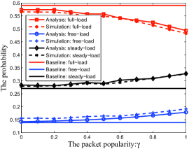
Figure 1: The probabilities of BSs in full-, modest- and free-load state for the caching network and the baseline. Note that previous studies consider all cells are active in full-load state, i.e., the probabilities of full-, modest- and free-load BSs are $\{100\%,0\%,0\%\}$.

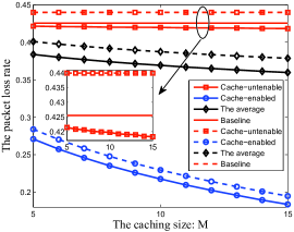
Figure 2: The packet loss rate with the change of caching size: solid lines are results of our analysis, dashed lines are that of previous studies regarding all cells are fully loaded. Note that for previous studies, the packet loss rate of the baseline overlaps with that of cache-untenable users [4, 5].

References

- [1] N. Golrezaei, A. Molisch, A. Dimakis, and G. Caire, “Femtocaching and device-to-device collaboration: A new architecture for wireless video distribution,” IEEE Commun. Mag., vol. 51, no. 4, pp. 142–149, Apr. 2013.
- [2] E. Baştuğ, M. Bennis, and M. Debbah, “Living on the Edge: The Role of Proactive Caching in 5G Wireless Networks,” IEEE Commun. Mag., vol. 52, no. 8, pp. 82–89, Aug. 2014.
- [3] A. Vinel, Q. Ni, D. Staehle, and A. Turlikov, “Capacity analysis of reservation-based random access for broadband wireless access networks,” IEEE J. Sel. Areas Commun., vol. 27, no. 2, pp. 172–181, Feb. 2009.
- [4] H.-S. Jo, Y. J. Sang, P. Xia, and J. Andrews, “Heterogeneous Cellular Networks with Flexible Cell Association: A Comprehensive Downlink SINR Analysis,” IEEE Trans. Wireless Commun., vol. 11, no. 10, pp. 3484–3495, Oct. 2012.
- [5] H. ElSawy, E. Hossain, and M. Haenggi, “Stochastic Geometry for Modeling, Analysis, and Design of Multi-Tier and Cognitive Cellular Wireless Networks: A Survey,” IEEE Commun. Surveys and Tutorials, vol. 15, no. 3, pp. 996–1019, June 2013.
- [6] B. Błaszczyszyn and A. Giovanidis, “Optimal Geographic Caching in Cellular Networks,” in Proc. ICC, June 2015.
- [7] E. Baştuğ, M. Bennis, K. Marios, and M. Debbah, “Cache-enabled small cell networks: modeling and tradeoffs,” EURASIP Journal on Wireless Commun. and Networking, Feb. 2015.
- [8] S. T. ul Hassan, M. Bennis, P. H. J. Nardelli, and M. Latva-aho, “Caching in Wireless Small Cell Networks: A Storage-Bandwidth Tradeoff,” IEEE Commun. Letters, vol. 20, no. 6, pp. 1175–1178, Mar. 2016.
- [9] A. Liu and V. K. N. Lau, “Mixed-Timescale Precoding and Cache Control in Cached MIMO Interference Network,” IEEE Trans. Signal Process., vol. 61, no. 24, pp. 6320–6332, Dec. 2013.
- [10] M. A. Maddah-Ali and U. Niesen, “Cache-Aided Interference Channels,” in ISIT, June 2015.
- [11] M. Deghel, E. BaŞtuğ, M. Assaad, and M. Débbah, “On the benefits of edge caching for MIMO interference alignment,” in Int’l Workshop on Signal Proc. Advances in Wireless Commun. (SPAWC), June 2015.
- [12] N. Naderializadeh, M. A. Maddah-Ali, and A. S. Avestimehr, “Fundamental Limits of Cache-Aided Interference Management,” in arXiv:1602.04207 [cs.IT], http://arxiv.org/abs/1602.04207, 2016.
- [13] M. Karray and M. Jovanovic, “A Queueing Theoretic Approach to the Dimensioning of Wireless Cellular Networks Serving Variable-Bit-Rate Calls,” IEEE Trans. Veh. Technol., vol. 62, no. 6, pp. 2713–2723, July 2013.
- [14] H. ElSawy and E. Hossain, “Two-Tier HetNets with Cognitive Femtocells: Downlink Performance Modeling and Analysis in a Multichannel Environment,” IEEE Trans. Mobile Computing, vol. 13, no. 3, pp. 649–663, Mar. 2014.
- [15] H. Bruneel, “A General Model for The Behaviour of Infinite Buffers with Periodic Service Opportunities,” European Journal of Operational Research, vol. 16, no. 1, pp. 98–106, 1984.