On time change equivalence of Borel flows

Abstract.

This paper addresses the notion of time change equivalence for Borel $\mathbb{R}^{d}$-flows. We show that all free $\mathbb{R}^{d}$-flows are time change equivalent up to a compressible set. An appropriate version of this result for non-free flows is also given.

1. Introduction

A Borel flow $\mathfrak{F}$ is a Borel measurable action of $\mathbb{R}^{d}$ on a standard Borel space. The action will be denoted additively: $x+\vec{r}$ is the action of $\vec{r}\in\mathbb{R}^{d}$ upon the point $x\in X$. With any flow $\mathfrak{F}$ on $X$ we associate an equivalence relation $\mathsf{E}_{X}^{\mathfrak{F}}$ given by $x\kern 1.0pt\mathsf{E}_{X}^{\mathfrak{F}}\kern 1.0pty$ whenever there is $\vec{r}\in\mathbb{R}^{d}$ such that $x+\vec{r}=y$. An equivalence class of $x\in X$ will be denoted by $[x]_{\mathsf{E}_{X}^{\mathfrak{F}}}$. An orbit equivalence between two flows $\mathbb{R}^{d}\curvearrowright X$ and $\mathbb{R}^{d}\curvearrowright Y$ is a Borel bijection $\phi:X\to Y$ such that for all $x,y\in X$

$$x\kern 1.0pt\mathsf{E}_{X}\kern 1.0pty\iff\phi(x)\kern 1.0pt\mathsf{E}_{Y}\kern 1.0pt\phi(y).$$

The notion of orbit equivalence is particularly suited for actions of discrete groups, but it tends to trivialize for certain locally compact groups. For instance, it is known that all non smooth free $\mathbb{R}^{d}$-flows are orbit equivalent. To remedy this collapse, one often considers various strengthenings of orbit equivalence, usually by imposing “local” restrictions on the orbit equivalence maps.

Given any orbit of a free action of $\mathbb{R}^{d}$, there is a bijective correspondence between points of the orbit and elements of $\mathbb{R}^{d}$. More precisely, with an equivalence relation $\mathsf{E}_{X}$ arising from a free flow $\mathbb{R}^{d}\curvearrowright X$ one may associate a cocycle map $\rho:\mathsf{E}_{X}\to\mathbb{R}^{d}$ which is defined by the condition

$$x+\rho(x,y)=y\quad\textrm{for all }x\kern 1.0pt\mathsf{E}_{X}\kern 1.0pty.$$

The map $\rho(x,\,\cdot\,)$ establishes a bijection between the orbit of $x$ and $\mathbb{R}^{d}$. While concrete identification depends on the choice of $x$, any translation invariant structure on $\mathbb{R}^{d}$ can be transferred onto orbits of such an action unambiguously. Time change equivalence between free flows is defined as an orbit equivalence that preserves the topology on every orbit.

Definition 1.1.

Let $\mathbb{R}^{d}\curvearrowright X$ and $\mathbb{R}^{d}\curvearrowright Y$ be free Borel flows. An orbit equivalence $\phi:X\to Y$ is said to be a time change equivalence if for any $x\in X$ the map $\xi(x,\,\cdot\,):\mathbb{R}^{d}\to\mathbb{R}^{d}$ specified by

$$\phi(x+\vec{r})=\phi(x)+\xi(x,\vec{r})$$

is a homeomorphism.

The concept of time change equivalence has been studied quite extensively in ergodic theory, where the set up differs from the one of Borel dynamics in the following aspects. In ergodic theory phase spaces are assumed to be endowed with probability measures, which flows are required to preserve (or to “quasi-preserve”, i.e., to preserve the null sets). Moreover, all conditions of interest may hold only up to a set of measure zero as opposed to holding everywhere. In these regards ergodic theory is less restrictive than Borel dynamics. On the other side, all orbit equivalence maps are additionally required to preserve measures between phases spaces, which significantly restricts the pool of possible orbit equivalences. In this aspect ergodic theory provides finer notions to differentiate flows. To summarize, frameworks of Borel dynamics and ergodic theory are in general positions, and while methods used in these areas are intricately related, there are oftentimes no direct implications between results.

In the measurable case, there is a substantial difference between one dimensional and higher dimensional $d\geq 2$ flows. There are continuumly many time change inequivalent $\mathbb{R}$-flows (see [ORW82]). In higher dimension the situation is simpler. Two relevant results here are due to D. Rudolph [Rud79] and J. Feldman [Fel91].

Theorem 1.2 (D. Rudolph).

Any two measure preserving ergodic $\mathbb{R}^{d}$-flows, $d\geq 2$, are time change equivalent.

Theorem 1.3 (J. Feldman).

Any two quasi measure preserving ergodic $\mathbb{R}^{d}$-flows, $d\geq 2$, are time change equivalent.

A striking difference of Borel framework was discovered in [MR10] by B. Miller and C. Rosendal, where they proved that all non smooth Borel $\mathbb{R}$-flows are time change equivalent. In other words, the flexibility of considering orbit equivalences which do not preserve any given measure turns out to be more important than the necessity to define equivalences on every orbit (as opposed to almost everywhere). We recall that an equivalence relation $\mathsf{E}$ on a standard Borel space $X$ is said to be smooth if there is a Borel map $f:X\to\mathbb{N}^{\mathbb{N}}$ such that

$$x\kern 1.0pt\mathsf{E}\kern 1.0pty\iff f(x)=f(y).$$

For equivalence relations arising as orbit equivalence relations of Polish group actions this is equivalent to existence of a Borel transversal — a Borel set that intersects each equivalence class in a single point.

Miller and Rosendal posed a question whether any two free Borel $\mathbb{R}^{d}$-flows are time change equivalent. This paper makes a contribution in this direction.

1.1. Main results

Many constructions in Borel dynamics and ergodic theory have to deal with two kinds of issues — “local” and “global”. Global aspects refer to properties that hold relative to many (usually all) orbits. Local aspects of a construction, on the other hand, reflect behavior that is local to any given orbit. For instance, the property of $\phi:X\to Y$ being an orbit equivalence between flows $\mathbb{R}^{d}\curvearrowright X$ and $\mathbb{R}^{d}\curvearrowright Y$ is global, as it requires different orbits to be mapped to different orbits. To be more specific, if a partial construction of $\phi$ yields $X\ni x\mapsto\phi(x)\in Y$ for some $x\in X$, then no $x^{\prime}\in X$ such that $\neg\bigl{(}x^{\prime}\kern 1.0pt\mathsf{E}_{X}\kern 1.0ptx\bigr{)}$ can be mapped into $\bigl{[}\phi(x)\bigr{]}_{\mathsf{E}_{Y}}$. In this sense, before defining $\phi(x^{\prime})$, any $x^{\prime}$ needs to know something about points $x\in X$ from other orbits. On the other hand, the property for an orbit equivalence $\phi:X\to Y$ to be a time change equivalence is purely local as it can be checked by looking at each orbit individually.

It is oftentimes beneficial (if nothing else for pedagogical reasons) to decouple whenever possible local and global aspects of a problem at hand. For various constructions of orbit equivalence this is achieved via the notion of a cross section.

Definition 1.4.

Let $\mathbb{R}^{d}\curvearrowright X$ be a Borel flow. A cross section for the flow is a Borel set $\mathcal{C}\subseteq X$ that intersects every orbit in a non-empty lacunary set, i.e., $\mathcal{C}\cap[x]_{\mathsf{E}_{X}}\neq\varnothing$ for all $x\in X$, and there is a non-empty neighborhood of the identity $U\subseteq\mathbb{R}^{d}$ such that $(x+U)\cap\mathcal{C}=\{x\}$ for all $x\in\mathcal{C}$. When one wants to specify $U$ explicitly, $\mathcal{C}$ is called $U$-lacunary.

One can think of a cross section as being a discrete version of the ambient equivalence relation. A theorem of A. S. Kechris [Kec92] shows that all Borel flows admit cross sections. The notion of a cross section can be further strengthened by requiring cocompactness.

Definition 1.5.

A cross section $\mathcal{C}$ for a flow $\mathbb{R}^{d}\curvearrowright X$ is cocompact if there exists a compact set $K\subseteq\mathbb{R}^{d}$ such that $\mathcal{C}+K=X$.

C. Conley proved existence of cocompact cross sections for all Borel flows (see, for instance, [Slu15, Section 2]). Our approach to separate local and global aspects of time change equivalence starts with cocompact cross sections $\mathcal{C}_{i}\subseteq X_{i}$ for two flows $\mathbb{R}^{d}\curvearrowright X_{i}$, $i=1,2$, and a given orbit equivalence $\phi:\mathcal{C}_{1}\to\mathcal{C}_{2}$. The question is then whether $\phi$ can be extended to a time change equivalence $\phi:X_{1}\to X_{2}$. Since $\phi$ is given on points from $\mathcal{C}_{1}$, its global behavior is uniquely defined, and one can concentrate on the local aspect of the problem. This approach is already implicit in the aforementioned work of Feldman [Fel91]. Before stating our results, we need one more definition.

Definition 1.6.

A Borel flow $\mathbb{R}^{d}\curvearrowright X$ is said to be compressible if it admits no invariant Borel probability measures. An invariant Borel subset $Z\subseteq X$ is compressible if the restriction of the flow onto $Z$ is compressible. An invariant set $Z\subseteq X$ is cocompressible if its complement is compressible.

The definition of compressibility given above is concise, but not very useful. The term “compressible” is explained by an important characterization due to M. G. Nadkarni [Nad90] (see also [BK96, Theorem 4.3.1]) of the direct analog of this notion for countable equivalence relations.

Our first result in this paper is the following theorem.

Theorem 1.7 (see Theorem 4.2).

Let $\mathbb{R}^{d}\curvearrowright X_{1}$ and $\mathbb{R}^{d}\curvearrowright X_{2}$, $d\geq 2$, be free non smooth Borel flows and let $\mathcal{D}_{i}\subseteq X_{i}$ be cocompact cross sections. For any orbit equivalence $\phi:\mathcal{D}_{1}\to\mathcal{D}_{2}$ there are cocompressible invariant Borel subsets $Z_{i}\subseteq X_{i}$ and a time change equivalence $\psi:Z_{1}\to Z_{2}$ which extends $\phi$ on $\mathcal{D}_{1}\cap Z_{1}$.

A corollary of the theorem above and of the classification of hyperfinite equivalence relations [DJK94] is time change equivalence of Borel $\mathbb{R}^{d}$-flows up to a compressible piece.

Theorem 1.8 (see Theorem 4.3).

Let $\mathbb{R}^{d}\curvearrowright X_{i}$, $i=1,2$, $d\geq 2$, be free non smooth Borel flows. There are cocompressible invariant Borel sets $Z_{i}\subseteq X$ such that the restrictions of flows onto these sets are time change equivalent.

In Section 5 we consider $\mathbb{R}^{d}$-flows that are not necessarily free. The main results therein are Theorem 5.1 and Theorem 5.4. The first one shows that one can identify any $\mathbb{R}^{d}$-flow with a number of free $\mathbb{R}^{p}\times\mathbb{T}^{q}$-flows, and the latter theorem establishes an analog of Theorem 4.2 in this more general context.

Finally, the last section, contains a remark on the difference between time change equivalence and Lebesgue orbit equivalence, which is defined as an orbit equivalence that preserves the Lebesgue measure between orbits. It illustrates the high complexity of Lebesgue orbit equivalence even in the simplest case of periodic $\mathbb{R}$-flows.

2. Rational Grids

This section provides some technical constructions that will be used in Section 4. The main concept here is that of a rational grid which will provide a rigorous justification for why the back-and-forth method in Section 4 can be performed in a Borel way.

Let $\mathbb{R}^{d}\curvearrowright X$ be a Borel flow. A spiral of cross sections $(\mathcal{C}_{n},h_{n})$, $n\in\mathbb{N}$, is a sequence of cross sections $\mathcal{C}_{n}$ together with Borel maps $h_{n}:\mathcal{C}_{n}\to\mathbb{R}^{d}$ such that $\mathcal{C}_{n+1}=\mathcal{C}_{n}+h_{n}$ for all $n\in\mathbb{N}$, i.e.,

$$\mathcal{C}_{n+1}=\{x+h_{n}(x):x\in\mathcal{C}_{n}\}.$$

With a spiral of cross sections we associate homomorphism maps

$$\phi_{n,n+1}:\mathcal{C}_{n}\to\mathcal{C}_{n+1}\quad\textrm{given by}\quad\phi_{n,n+1}(x)=x+h_{n}(x),$$

and $\phi_{k,n}:\mathcal{C}_{k}\to\mathcal{C}_{n}$ for $k\leq n$ defined as

$$\phi_{k,n}=\phi_{n-1,n}\circ\phi_{n-2,n-1}\circ\cdots\circ\phi_{k,k+1}$$

with the agreement that $\phi_{n,n}:\mathcal{C}_{n}\to\mathcal{C}_{n}$ is the identity map. Note that

$$\phi_{m,n}\circ\phi_{k,m}=\phi_{k,n}\quad\textrm{for all }k\leq m\leq n.$$

When a flow $\mathfrak{F}$ on $X$ is free, one has a cocycle $\rho:\mathsf{E}_{X}\to\mathbb{R}^{d}$ that assigns to a pair $(x,y)\in\mathsf{E}_{X}$ the unique vector $\vec{r}\in\mathbb{R}^{d}$ such that $x+\vec{r}=y$. If $(\mathcal{C}_{n},h_{n})$ is a spiral of cross sections for $\mathfrak{F}$, then for all $x\in\mathcal{C}_{0}$

(†) $$\rho\bigl{(}x,\phi_{0,n}(x)\bigr{)}=h_{0}(x)+h_{1}\bigl{(}\phi_{0,1}(x)\bigr{)}+\cdots+h_{n-2}\bigl{(}\phi_{0,n-2}(x)\bigr{)}+h_{n-1}\bigl{(}\phi_{0,n-1}(x)\bigr{)}.$$

A spiral of cross sections $(\mathcal{C}_{n},h_{n})$, $n\in\mathbb{N}$, of a free flow is said to be convergent if for all $x\in\mathcal{C}_{0}$ the limit $\lim_{n}\rho\bigl{(}x,\phi_{0,n}(x)\bigr{)}$ exists. For a convergent spiral we define the limit shift maps $H_{k}:\mathcal{C}_{k}\to\mathbb{R}^{d}$ by

$$H_{k}(x)=\lim_{n\to\infty}\Bigl{[}h_{k}(x)+h_{k+1}\bigl{(}\phi_{k,k+1}(x)\bigr{)}+\cdots+h_{n-2}\bigl{(}\phi_{k,n-2}(x)\bigr{)}+h_{n-1}\bigl{(}\phi_{k,n-1}(x)\bigr{)}\Bigr{]}.$$

Being a pointwise limit of Borel functions, $H_{k}$ is Borel. The limit cross section of a convergent spiral is a set $\mathcal{D}\subseteq X$ defined by

$$\mathcal{D}=\mathcal{C}_{0}+H_{0}=\{x+H_{0}(x):x\in\mathcal{C}_{0}\}.$$

Note that $\mathcal{D}=\mathcal{C}_{k}+H_{k}$ for any $k\in\mathbb{N}$. Also, we let $\phi_{k,\infty}:\mathcal{C}_{k}\to\mathcal{D}$ to be $\phi_{k,\infty}(x)=x+H_{k}(x)$. The set $\mathcal{D}$ is necessarily Borel, as it is a countable-to-one image of a Borel function. In general, $\mathcal{D}$ may not be lacunary, but the following easy conditions guarantee lacunarity of the limit cross section. Hereafter $B(\delta)\subseteq\mathbb{R}^{d}$ denotes an open ball of radius $\delta$ around the origin.

Proposition 2.1.

Let $\mathfrak{C}=(\mathcal{C}_{n},h_{n})$, $n\in\mathbb{N}$, be a spiral of cross sections for a free flow $\mathbb{R}^{d}\curvearrowright X$. If there exists a convergent series $\sum_{i=0}^{\infty}a_{i}$ of positive reals such that $h_{n}:\mathcal{C}_{n}\to B(a_{i})$, then the spiral $\mathfrak{C}$ is convergent. If furthermore $\mathcal{C}_{0}$ is $B(\delta)$-lacunary for some $\delta$ such that $\sum_{i}a_{i}<\delta$, then the limit cross section of the spiral is $B\bigl{(}\delta-\sum_{i}a_{i}\bigr{)}$-lacunary.

Proof.

The proof is immediate from the equation († ‣ 2). ∎

Definition 2.2.

A rational grid for a flow $\mathbb{R}^{d}\curvearrowright X$ is a Borel subset $Y\subseteq X$ which is invariant under the action of $\mathbb{Q}^{d}$ and intersects every orbit of the flow in a unique $\mathbb{Q}^{d}$-orbit: for every $x\in X$ there is $y\in Y$ such that $[x]_{\mathbb{R}^{d}}\cap Y=[y]_{\mathbb{Q}^{d}}$.

Lemma 2.3.

Any free Borel flow admits a rational grid.

Proof.

For every $\epsilon>0$ we pick a Borel map $\alpha_{\epsilon}:\mathbb{R}^{d}\to\mathbb{Q}^{d}$ such that $\bigl{|}\bigl{|}\vec{r}-\alpha_{\epsilon}(\vec{r})\bigr{|}\bigr{|}<\epsilon$ for all $\vec{r}\in\mathbb{R}^{d}$. By a theorem of Kechris [Kec92], there exists a $B(2)$-lacunary cross section $\mathcal{C}\subseteq X$. Restriction $\mathsf{E}_{\mathcal{C}}$ of the orbit equivalence relation onto $\mathcal{C}$ is hyperfinite (see [JKL02, Theorem 1.16]), and one may therefore represent $\mathsf{E}_{\mathcal{C}}$ as an increasing union of finite equivalence relations: $\mathsf{E}_{\mathcal{C}}=\bigcup_{n}\mathsf{F}_{m}$.

We are going to construct a spiral of cross sections $(C_{n},h_{n})$, $n\in\mathbb{N}$, $\mathcal{C}_{0}=\mathcal{C}$, such that $h_{n}:\mathcal{C}_{n}\to B\bigl{(}2^{-n-1}\bigr{)}$. Let $\mathsf{F}_{m}^{n}$ denote the equivalence relation $\mathsf{F}_{m}$ transferred onto $\mathcal{C}_{n}$ via $\phi_{0,n}$:

$$x\kern 1.0pt\mathsf{F}_{m}^{n}\kern 1.0pty\iff\phi^{-1}_{0,n}(x)\kern 1.0pt\mathsf{F}_{m}\kern 1.0pt\phi^{-1}_{0,n}(y).$$

The spiral will satisfy the following two conditions:

1. $h_{n}$ is constant on $\mathsf{F}_{n-1}^{n}$-equivalence classes:

   $$x\kern 1.0pt\mathsf{F}_{n-1}^{n}\kern 1.0pty\implies h_{n}(x)=h_{n}(y).$$

2. Every $\mathsf{F}_{n-1}^{n}$ class in $\mathcal{C}_{n}$ is “on a rational grid:”

   $$x\kern 1.0pt\mathsf{F}_{n-1}^{n}\kern 1.0pty\implies\rho(x,y)\in\mathbb{Q}^{d}.$$

To this end pick a Borel linear ordering $\prec$ on $X$. For the base of construction we set $\mathcal{C}_{0}=\mathcal{C}$; let $s_{0}:\mathcal{C}_{0}\to\mathcal{C}_{0}$ be the Borel selector that picks the $\prec$-minimal element within $\mathsf{F}_{0}^{0}$-classes, and define $h_{0}:\mathcal{C}_{0}\to B(1/2)$ to be

$$h_{0}(x)=\alpha_{1/2}\bigl{(}\rho\bigl{(}s_{0}(x),x\bigr{)}\bigr{)}-\rho\bigl{(}s_{0}(x),x\bigr{)}.$$

The cross section $\mathcal{C}_{1}$ is then the $h_{0}$-shift of $\mathcal{C}_{0}$: $\mathcal{C}_{1}=\bigl{\{}x+h_{0}(x):x\in\mathcal{C}_{0}\bigr{\}}$. Geometrically, $\mathcal{C}_{1}$ is constructed by shifting points by at most $1/2$ within $\mathsf{F}_{0}^{0}$-classes relative to the origin provided by the minimal point $s_{0}(x)$.

The inductive step is very similar, with a notable difference lying in the fact that when moving points within each $\mathsf{F}_{n}^{n}$-class, together with any point we move its $\mathsf{F}_{n-1}^{n}$-class. More precisely, suppose $\mathcal{C}_{n},h_{n-1}$ have been constructed, and let $s_{n}:\mathcal{C}_{n}\to\mathcal{C}_{n}$ be the Borel selector, which picks $\prec$-minimal points within $\mathsf{F}_{n}^{n}$-classes. Let also $\tilde{s}_{n-1}:\mathcal{C}_{n}\to\mathcal{C}_{n}$ denote the Borel selector for $\mathsf{F}_{n-1}^{n}$-classes. Define $h_{n}:\mathcal{C}_{n}\to B\bigl{(}2^{-n-1}\bigr{)}$ by setting

$$h_{n}(x)=\alpha_{2^{-n-1}}\bigl{(}\rho\bigl{(}s_{n}(x),\tilde{s}_{n-1}(x)\bigr{)}\bigr{)}-\rho\bigl{(}s_{n}(x),\tilde{s}_{n-1}(x)\bigr{)}.$$

It is easy to see that items (1) and (2) are satisfied. Also, $h_{n}:\mathcal{C}_{n}\to B(2^{-n-1})$ and Proposition 2.1 ensure that $(\mathcal{C}_{n},h_{n})$ converges, and the limit cross section $\mathcal{D}$ is $B(1)$-lacunary. We claim that $\mathcal{D}$ is on a rational grid in the sense that $\rho(x,y)\in\mathbb{Q}^{d}$ for all $x,y\in\mathcal{D}$ such that $x\kern 1.0pt\mathsf{E}_{X}\kern 1.0pty$. Indeed, let $m$ be so large that $\phi_{0,\infty}^{-1}(x)\kern 1.0pt\mathsf{F}_{m}^{0}\kern 1.0pt\phi_{0,\infty}^{-1}(y)$, and therefore also

$$\phi_{m+1,\infty}^{-1}(x)\kern 1.0pt\mathsf{F}_{m}^{m+1}\kern 1.0pt\phi_{m+1,\infty}^{-1}(y).$$

Item (2) implies that

$$\vec{q}:=\rho\bigl{(}\phi_{m+1,\infty}^{-1}(x),\phi_{m+1,\infty}^{-1}(y)\bigr{)}\in\mathbb{Q}^{d}.$$

It now follows from item (1) and the definition of the limit cross section that $\rho(x,y)=\vec{q}$ and thus $\rho(x,y)\in\mathbb{Q}^{d}$ as claimed.

The required rational grid is given by $\mathcal{D}+\mathbb{Q}^{d}$.

∎

Let $Q$ be a rational grid for a Borel flow $\mathbb{R}^{d}\curvearrowright X$. We say that a cross section $\mathcal{C}$ is on the grid $Q$ if $\mathcal{C}\subseteq Q$. A small perturbation allows one to shift any cross section to a given grid.

Lemma 2.4.

Let $Q\subseteq X$ be a rational grid for a free flow $\mathbb{R}^{d}\curvearrowright X$. For any cross section $\mathcal{C}\subseteq X$ and any $\epsilon>0$ there exist a cross section $\mathcal{C}^{\prime}$ on the grid $Q$ and a Borel orbit equivalence $\phi:\mathcal{C}\to\mathcal{C}^{\prime}$ such that $\bigl{|}\bigl{|}\rho\bigl{(}x,\phi(x)\bigr{)}\bigr{|}\bigr{|}<\epsilon$ for all $x\in\mathcal{C}$.

Proof.

Let $\delta>0$ be so small that $\mathcal{C}$ is $B(\delta)$-lacunary. We may assume without loss of generality that $\epsilon<\delta$. Let $P\subseteq\mathcal{C}\times Q$ be the set

$$P=\bigl{\{}(x,y)\in\mathcal{C}\times Q:x\kern 1.0pt\mathsf{E}_{X}\kern 1.0pty\textrm{ and }||\rho(x,y)||<\epsilon\bigr{\}}.$$

Clearly, $\operatorname{proj}_{\mathcal{C}}(P)=\mathcal{C}$. Since the projection of $P$ onto the first coordinate is countable-to-one, Luzin–Novikov Theorem (see [Kec95, 18.14]) guarantees existence of a Borel “inverse”, i.e., a Borel map $\phi:\mathcal{C}\to Q$ such that $\bigl{(}c,\phi(c)\bigr{)}\in P$ for all $c\in\mathcal{C}$. The map $\phi$ is injective, since $\epsilon<\delta$. The required cross section $\mathcal{C}^{\prime}$ is given by $\phi(\mathcal{C})$. ∎

3. Some Simple Tools

In this section we gather a few elementary tools that will be useful in the proof of the main theorem.

Lemma 3.1 (Small perturbation lemma).

Let $\mathbb{R}^{d}\curvearrowright X$ be a free Borel flow, let $\mathcal{C},\mathcal{D}\subseteq X$ be Borel cross sections, and let $\phi:\mathcal{C}\to\mathcal{D}$ be an orbit equivalence. If $\mathcal{C}$ is $B(\delta)$-lacunary for some $\delta>0$ and

$$\bigl{|}\bigl{|}\rho\bigl{(}x,\phi(x)\bigr{)}\bigr{|}\bigr{|}<\delta\quad\textrm{for all}\quad x\in\mathcal{C},$$

then there exists a time change equivalence $\psi:X\to X$ that extends $\phi$.

Proof.

For any $\vec{r}$ in $B(\delta)\subset\mathbb{R}^{d}$ there exists a diffeomorphism $f_{\vec{r}}:B(\delta)\to B(\delta)$ with compact support such that $f_{\vec{r}}(\vec{0})=\vec{r}$. The proof of this assertion is sufficiently concrete (see e.g., [Mil97, p. 22]), so that the dependence on $\vec{r}$ is Borel, i.e., one can pick a Borel map $f:B(\delta)\times B(\delta)\to B(\delta)$ such that $f(\vec{r},\,\cdot\,):B(\delta)\to B(\delta)$ is a compactly supported diffeomorphism, and $f(\vec{r},\vec{0})=\vec{r}$ for all $\vec{r}\in B(\delta)$.

Let $\xi:\mathcal{C}+B(\delta)\to\mathcal{C}$ be the map given by $\xi(x+\vec{r})=x$ for all $x\in\mathcal{C}$ and $\vec{r}\in B(\delta)$. The required time change equivalence $\psi:X\to X$ is defined by the formula:

$$\psi(x)=\begin{cases}x&\textrm{if }x\not\in\mathcal{C}+B(\delta),\\ \xi(x)+f\bigl{(}\rho\bigl{(}\xi(x),\phi\circ\xi(x)\bigr{)},\rho\bigl{(}\xi(x),x\bigr{)}\bigr{)}&\textrm{otherwise}.\\ \end{cases}$$

The somewhat cryptic definition of $\psi(x)$ is really simple: within a ball $c+B(\delta)$, $c\in\mathcal{C}$, we apply the diffeomorphism $f(\vec{r},\,\cdot\,)$, $\vec{r}=\rho(c,\phi(c))$, ensuring that $\psi(c)=\phi(c)$. By assumption $\mathcal{C}$ is $B(\delta)$-lacunary, and therefore $\psi$ is injective, and hence is a time change equivalence. ∎

One of the primary tools to construct orbit equivalences is Rokhlin’s Lemma. The following provides a concrete form that we are going to use. The statement essentially coincides with that of Theorem 6.3 in [Slu15] with addition of item (v), which asserts that cross section $\mathcal{C}_{n}$ can be taken to be on the given grid $Q$. This modification is straightforward in view of Lemma 3.1 above.

Lemma 3.2.

For any free Borel flow $\mathbb{R}^{d}\curvearrowright X$ and any rational grid $Q\subseteq X$ there exist a Borel cocompressible invariant set $Z\subseteq X$, a sequence of Borel cross sections $\mathcal{C}_{n}\subseteq Z$, and an increasing sequence of positive rationals $(l_{n})_{n=1}^{\infty}$ such that for rectangles $R_{n}=[-l_{n},l_{n}]^{d}$ one has:

1. $\lim_{n\to\infty}l_{n}=\infty$;

2. $Z=\bigcup_{n}\bigl{(}\mathcal{C}_{n}+R_{n}\bigr{)}$;

3. $(c+R_{n})\cap(c^{\prime}+R_{n})=\varnothing$ for all distinct $c,c^{\prime}\in R_{n}$;

4. $\mathcal{C}_{n}+R_{n}\subseteq\mathcal{C}_{n+1}+R_{n+1}^{\leftarrow 1}$, where $R_{n+1}^{\leftarrow 1}$ is obtained by shrinking the square $R_{n+1}$ by $1$ in every direction:

   $$R_{n+1}^{\leftarrow 1}=[-l_{n+1}+1,l_{n+1}-1]^{d};$$

5. $\mathcal{C}_{n}\subseteq Q$.

For any flow $\mathbb{R}^{d}\curvearrowright X$, we let $\mathcal{E}(X)$ to denote the Borel space of invariant ergodic probability measures on $X$. The construction of the time change equivalence given in Section 4 would be easier if performed relative to a fixed ergodic measure on $X$. To make it work generally, we make use of the following classical ergodic decomposition theorem due to Varadarajan.

Lemma 3.3 (Ergodic Decomposition).

For any free Borel flow $\mathbb{R}^{d}\curvearrowright X$ with $\mathcal{E}(X)\neq\varnothing$ there exists a Borel surjection $x\mapsto\mu_{x}$ from $X$ onto $\mathcal{E}(X)$ such that

1. $x\kern 1.0pt\mathsf{E}_{X}\kern 1.0pty\implies\mu_{x}=\mu_{y}$;

2. $\nu\bigl{(}\bigl{\{}x:\mu_{x}=\nu\bigr{\}}\bigr{)}=1$ for any $\nu\in\mathcal{E}(X)$.

The following extension lemma will be used routinely through the back-and-forth construction. It is taken directly from [Fel91, Proposition 2.6].

Lemma 3.4 (Extension Lemma).

Let $R,R^{\prime}$ and $D_{i},D_{i}^{\prime}\subseteq\mathbb{R}^{d}$, $1\leq i\leq n$, be smooth disks such that $D_{i}\subseteq R$ and $D_{i}^{\prime}\subseteq R^{\prime}$. Any family of orientation preserving diffeomorphisms $f_{i}:D_{i}\to D_{i}^{\prime}$ admits a common extension to an orientation preserving diffeomorphism $f:R\to R^{\prime}$.

Finally, we shall need the following easy fact from the theory of countable Borel equivalence relations.

Lemma 3.5.

Let $\mathsf{E},\mathsf{F}$ be finite Borel equivalence relation on a standard Borel space $X$. Suppose that $\mathsf{F}\subseteq\mathsf{E}$. There is a sequence of disjoint Borel sets $A_{n}\subseteq X$ such that

1. $X=\bigsqcup_{n}A_{n}$;

2. each $A_{n}$ is $\mathsf{F}$-invariant;

3. $[x]_{\mathsf{E}}\cap A_{n}=[x]_{\mathsf{F}}$ for all $x\in A_{n}$.

If there is a bound on $[\mathsf{F}:\mathsf{E}]$ — the number of $\mathsf{F}$-classes in a $\mathsf{E}$-class — then the sequence $(A_{n})_{n}$ can be taken to be finite.

Proof.

Since $\mathsf{E}$ is smooth, it admits a Borel transversal $B_{0}\subseteq X$. Set $A_{0}=[B_{0}]_{\mathsf{F}}$, and set recursively $A_{n}=[B_{n}]_{\mathsf{F}}$, where $B_{n}$ is a Borel transversal for $\mathsf{E}$ restricted onto $X\setminus\bigcup_{k<n}A_{k}$. ∎

4. Back and forth construction

For the proof of the following theorem it is convenient to introduce the notion of a tree of partitions. Let $\mathbb{R}^{d}\curvearrowright X$ be a free flow on $X$. A tree of partitions for the flow is a family of invariant Borel sets $(\Omega_{s})_{s\in\mathbb{N}^{<\mathbb{N}}}$, $\Omega_{s}\subseteq X$, indexed by finite sequences of natural numbers that satisfies the following two conditions:

1. $X=\bigsqcup_{s\in\mathbb{N}^{n}}\Omega_{s}$ for each $n\in\mathbb{N}$; in particular, $\Omega_{\varnothing}=X$.

2. $s\subseteq t\implies\Omega_{t}\subseteq\Omega_{s}$.

Theorem 4.1.

Let $\mathbb{R}^{d}\curvearrowright X_{1}$ and $\mathbb{R}^{d}\curvearrowright X_{2}$ be free Borel flows on standard Borel spaces, let for $i=1,2$, $Q_{i}\subseteq X_{i}$ be rational grids, let $\mathcal{D}_{i}\subseteq Q_{i}$ be cocompact cross sections on these grids, and let $\zeta:\mathcal{D}_{1}\to\mathcal{D}_{2}$ be an orbit equivalence between them. There are Borel invariant cocompressible sets $Z_{i}\subseteq X_{i}$, and a time change equivalence $\psi:Z_{1}\to Z_{2}$ that extends $\zeta$, i.e., $\zeta|_{Z_{1}\cap\mathcal{D}_{1}}=\psi|_{Z_{1}\cap\mathcal{D}_{1}}$.

Proof.

The proof relies on a back-and-forth argument similar to the one used in the proof of Theorem 1 in [Fel91]. For start, let us apply the Uniform Rokhlin Lemma (Lemma 3.2) to both flows yielding Borel invariant cocompressible sets $\tilde{Z}_{i}\subseteq X_{i}$, as well as cross sections $\mathcal{C}_{i,n}\subseteq\tilde{Z}_{i}$ , $n\in\mathbb{N}$, and rationals $l_{i,n}\in\mathbb{Q}$ such that for the squares $R_{i,n}=[-l_{i,n},l_{i,n}]^{d}$ , $i=1,2$, one has

1. cross sections $\mathcal{C}_{i,n}\subseteq Q_{i}$ are on the rational grids;

2. $\tilde{Z}_{i}=\bigcup_{n}\bigl{(}\mathcal{C}_{i,n}+R_{i,n}\bigr{)}$;

3. boxes $c+R_{i,n}$ are pairwise disjoint;

4. $\mathcal{C}_{i,n}+R_{i,n}\subseteq\mathcal{C}_{i,n+1}+R_{i,n+1}^{\leftarrow 1}$;

5. sequences $(l_{i,n})_{n\in\mathbb{N}}$ are increasing and unbounded.

Since cross sections $\mathcal{D}_{i}$ are cocompact, we may omit, if necessary, finitely many cross sections $\mathcal{C}_{i,n}$ and assume without loss of generality that $l_{i,n}$ are so large that $\mathcal{D}_{i}\cap(c+R_{i,n})\neq\varnothing$ for all $c\in\mathcal{C}_{i,n}$. We shall further decrease sets $\tilde{Z}_{i}$ by throwing away invariant compressible sets, so for notational convenience we assume that $\tilde{Z}_{i}=X_{i}$.

For each of $X_{i}$ we pick an ergodic decomposition $x\mapsto\mu_{x}$ as in Lemma 3.3. We also let $\mathsf{F}_{n}^{i}$ to denote finite Borel equivalence relations on $\mathcal{D}_{i}\cap\bigl{(}\mathcal{C}_{i,n}+R_{i,n}\bigr{)}$ given by

$$x\kern 1.0pt\mathsf{F}_{n}^{i}\kern 1.0pty\iff x,y\in(c+R_{i,n})\quad\textrm{for some }c\in\mathcal{C}_{i,n}.$$

Each $\kern 1.0pt\mathsf{F}_{n}^{i}\kern 1.0pt$ class lives in a unique $R_{i,n}$ box. We are going to construct trees of Borel partitions $(\Omega_{i,s})_{s\in\mathbb{N}^{<\mathbb{N}}}$ on $X_{i}$, together with families of positive integers $(\omega_{i,s})_{s\in\mathbb{N}^{<\mathbb{N}}}$. Before listing properties of these objects, let us introduce the following sets:

$$\mathcal{V}_{1,s}=\bigl{\{} x\in\mathcal{C}_{1,\omega_{1,s}}:\textrm{for all }y_{1},y_{2}\in\mathcal{D}_{1}\cap\bigl{(}x+R_{1,\omega_{1,s}}\bigr{)}$$

$$\textrm{one has }\zeta(y_{1}){\kern 1.0pt\mathsf{F}_{\omega_{2,s}}^{2}\kern 1.0pt}\zeta(y_{2})\bigr{\}},$$

$$\mathcal{V}_{2,s}=\bigl{\{} x\in\mathcal{C}_{2,\omega_{2,s}}:\textrm{for all }y_{1},y_{2}\in\mathcal{D}_{2}\cap\bigl{(}x+R_{2,\omega_{2,s}}\bigr{)}$$

$$\textrm{one has }\zeta^{-1}(y_{1}){\kern 1.0pt\mathsf{F}_{\omega_{1,s}}^{1}\kern 1.0pt}\zeta^{-1}(y_{2})\bigr{\}}.$$

Figure 1 illustrates the definition of the set $\mathcal{V}_{1,s}$: a point $x\in\mathcal{C}_{1,\omega_{1,s}}$ belongs to $\mathcal{V}_{1,s}$ if the images under $\zeta$ of all the points of $\mathcal{D}_{1}$ in the box $R_{1,\omega_{1,s}}$ around $x$ fall into a single box $R_{2,\omega_{2,s}}$ in $X_{2}$. The definition of $\mathcal{V}_{2,s}$ uses $\zeta^{-1}$ instead of $\zeta$.

Figure 1. Definition of sets $\mathcal{V}_{i,s}$.

The role of integers $\omega_{i,s}$ will be to ensure that sets $\mathcal{V}_{i,s}$ are sufficiently large in measure.

We are now ready to list the conditions on the trees of Borel partitions $\Omega_{i,s}$ and natural $\omega_{i,s}$.

1. Sets $\Omega_{i,s}$ are invariant with respect to the ergodic decompositions, i.e., $\mu_{x}=\mu_{y}$ and $x\in\Omega_{i,s}$ implies $y\in\Omega_{i,s}$.

2. $\omega_{i,s}\geq|s|$;

3. $s\subseteq t$ implies $\omega_{i,s}\leq\omega_{i,t}$;

4. If $|s|$ is odd, then for any $x\in\Omega_{1,s}$ one has $\mu_{x}\bigl{(}\mathcal{V}_{1,s}+R_{1,\omega_{1,s}}\bigr{)}\leq 2^{-|s|}$; if $|s|$ is even, then

   $$\mu_{x}\bigl{(}\mathcal{V}_{2,s}+R_{2,\omega_{2,s}}\bigr{)}\leq 2^{-|s|}\textrm{ for all }x\in\Omega_{2,s}.$$

Let us first finish the argument under the assumption that such objects have been constructed. The base of the inductive construction is the map

$$\psi_{1}:\bigcup_{s\in\mathbb{N}^{1}}\bigl{(}\mathcal{V}_{1,s}+R_{1,\omega_{1,s}}\bigr{)}\to X_{2},$$

which will be an orientation preserving diffeomorphism between orbits on its domain. Pick some $s\in\mathbb{N}^{1}$, and define $\psi_{1}$ on $\mathcal{V}_{1,s}+R_{1,\omega_{1,s}}$ as follows.

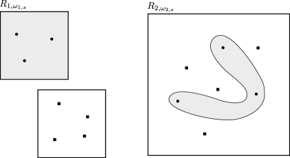
Figure 2. Extension step

To a point $x\in\mathcal{V}_{1,s}$ there corresponds a box $x+R_{1,\omega_{1,s}}$, marked gray in Figure 2, which contains several points, say $y_{1},\ldots,y_{m}\in\mathcal{D}_{1}$. Images of these points, $\zeta(y_{1}),\ldots,\zeta(y_{m})$, fall into a single $z+R_{2,\omega_{2,s}}$ box, $z\in\mathcal{C}_{2,\omega_{2,s}}$. Besides points $\zeta(y_{1}),\ldots,\zeta(y_{m})$, the box $z+R_{2,\omega_{2,s}}$ may contain other points of $\mathcal{D}_{2}$. We pick any smooth disk inside $z+R_{2,\omega_{2,s}}$ that contains all the points $\zeta(y_{1}),\ldots,\zeta(y_{m})$ and does not contain any other points of $\mathcal{D}_{2}$. One now would like to extend the map

$$\zeta:\bigl{\{}y_{1},\ldots,y_{m}\bigr{\}}\to\bigl{\{}\zeta(y_{1}),\ldots,\zeta(y_{m})\bigr{\}}$$

to an orientation preserving diffeomorphism $\psi_{1}$ from $x+R_{1,\omega_{1,s}}$ to the smooth disk around $\zeta(y_{1}),\ldots,z(y_{m})$. This can be done by the Extension Lemma 3.4 (the fact that $\zeta$ is defined on points rather than disks is, of course, immaterial, as is the fact that $R_{1,\omega_{1,s}}$ is not a smooth disk, since it has corners; to be pedantic, one extends $\zeta$ to little balls around points in $\mathcal{D}_{i}$ in a linear fashion, and considers $\tilde{R}_{i,\omega_{i,s}}\subseteq R_{i,\omega_{i,s}}$ — “rectangles with smoothed corners” instead). The problem that arises with the use of Extension Lemma is the following one. The construction needs to be performed in a Borel way, meaning that extension $\psi_{1}$ has to be defined for boxes $x+R_{1,\omega_{1,s}}$ for all $x\in\mathcal{V}_{1,s}$ at the same time, which can possibly lead to “collisions” and prevent $\psi_{1}$ from being injective. For instance, in Figure 2 there are two distinct $R_{1,\omega_{1,s}}$ boxes that must be mapped into a single $R_{2,\omega_{2,s}}$ box, so we need to ensure that their images are disjoint. The way to do this is to partition $\mathcal{V}_{1,s}$ into finitely many Borel pieces $\mathcal{V}_{1,s}=A_{1}\sqcup\cdots\sqcup A_{p}$ such that on each $A_{j}$ every $R_{1,\omega_{1,s}}$ box corresponds to a unique square $R_{2,\omega_{2,s}}$ via $\zeta$. To this end consider an equivalence relation $\mathsf{E}$ on $\mathcal{D}_{1}\cap\bigl{(}\mathcal{V}_{1,s}+R_{1,\omega_{1,s}}\bigr{)}$ given by

$$x\kern 1.0pt\mathsf{E}\kern 1.0pty\iff\zeta(x)\kern 1.0pt\mathsf{F}_{\omega_{2,s}}^{2}\kern 1.0pt\zeta(y),$$

and let $\mathsf{F}$ denote the restriction of $\mathsf{F}_{\omega_{1,s}}^{1}$ onto $\mathcal{D}_{1}\cap\bigl{(}\mathcal{V}_{1,s}+R_{1,\omega_{1,s}}\bigr{)}$. By the definition of $\mathcal{V}_{1,s}$ one has $\mathsf{F}\subseteq\mathsf{E}$, so Lemma 3.5 applies, and gives a partition

$$\mathcal{D}_{1}\cap\bigl{(}\mathcal{V}_{1,s}+R_{1,\omega_{1,s}}\bigr{)}=\bigsqcup_{j=1}^{p}A_{j}^{\prime}.$$

The required partition of $\mathcal{V}_{1,s}$ is obtained by setting

$$A_{j}=\{ x\in\mathcal{V}_{1,s}:y\in A_{j}^{\prime}\textrm{ for some (equivalently, any) }y\in\mathcal{D}_{1}$$

$$\textrm{such that }y\in x+R_{1,\omega_{1,s}}\}.$$

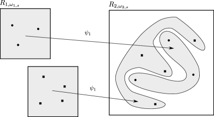
Figure 3. Extension

We can now define the extension $\psi_{1}$ with domain $A_{1}+R_{1,\omega_{1,s}}$ as explained above, which is guaranteed to be injective. Next we extend $\psi_{1}$ to $A_{2}+R_{1,\omega_{1,s}}$ in a similar way (Figure 3). Given $x^{\prime}\in A_{2}$ and points $y^{\prime}_{1},\ldots,y^{\prime}_{q}\in\mathcal{D}_{1}\cap\bigl{(}x^{\prime}+R_{1,\omega_{1,s}}\bigr{)}$, let $z^{\prime}\in\mathcal{C}_{2,\omega_{2,s}}$ be such that $\zeta(y^{\prime}_{j})\in z^{\prime}+R_{2,\omega_{2,s}}$ for all $j$. Pick a smooth disk inside $z^{\prime}+R_{2,\omega_{2,s}}$ that contains all the points $\zeta(y^{\prime}_{j})$, does not contain any other points of $\mathcal{D}_{2}$, and does not intersect any smooth disks inside $z^{\prime}+R_{2,\omega_{2,s}}$ picked at the previous step. One may now use the Extension Lemma to extend $\psi_{1}$ to a map

$$\psi_{1}:(A_{1}\cup A_{2})+R_{1,\omega_{1,s}}\to\mathcal{C}_{2,\omega_{2,s}}+R_{2,\omega_{2,s}}.$$

Continuing in the same fashion, $\psi_{1}$ can be extended to all of $\mathcal{V}_{1,s}+R_{1,\omega_{1,s}}$.

The construction above was performed for a fixed $s\in\mathbb{N}^{1}$, doing it for all $s\in\mathbb{N}^{1}$ results in the required map

$$\psi_{1}:\bigcup_{s\in\mathbb{N}^{1}}\bigl{(}\mathcal{V}_{1,s}+R_{1,\omega_{1,s}}\bigr{)}\to\bigcup_{s\in\mathbb{N}^{1}}\bigl{(}\mathcal{C}_{2,\omega_{2,s}}+R_{2,\omega_{2,s}}\bigr{)}.$$

We have explained the way $\psi_{1}$ is defined, but we owe the reader an explanation why this construction is Borel. This is the place where we are going to use rational grids. Since all cross sections $\mathcal{C}_{i,n}$, $\mathcal{D}_{i}$ are assumed to be on the rational grid $Q_{i}$, at each step of the construction, every box of the form $x+R_{i,\omega_{i,s}}$, $x\in\mathcal{C}_{i,n}$, has only countable many possible configurations. For example, for any $x\in A_{1}$ the configuration of $\mathcal{D}_{1}\cap\bigl{(}x+R_{1,\omega_{1,s}}\bigr{)}$ is uniquely determined by the vectors $\rho(y_{i},x)\in\mathbb{Q}^{d}$. Since we have only countably many possible configurations, we can partition $A_{1}$ into countably many pieces by collecting points with the same configuration of boxes around them, and apply the same extension of $\psi_{1}$ on each element of this partition. Such an operation is clearly Borel for any choice of smooth disks around points $y_{1},\ldots,y_{m}$, any choice of smooth extensions given by Lemma 3.4, etc. Thus having only countably many cases at each step of the back-and-forth construction ensures Borelness.

We are now done with the base step of the construction. The inductive step is of little difference. At step $n$ for an odd value of $n$, $\psi_{n}$ is constructed such that $\mathcal{V}_{1,s}+R_{1,\omega_{1,s}}$ is in the domain of $\psi_{n}$ for all $s\in\mathbb{N}^{n}$, and on even stages we work with $\zeta^{-1}$, ensuring that $\mathcal{V}_{2,s}+R_{2,\omega_{2,s}}$ is in the range of $\psi_{n}$ for all $s\in\mathbb{N}^{n}$. Item (4) in the list of conditions on the sets $\mathcal{V}_{i,s}$ guarantees that sets

$$Z_{1} =\bigcup_{m\in\mathbb{N}}\mkern-6.0mu\bigcap_{|s|\geq m\atop|s|\textrm{ is odd}}\mkern-8.0mu\bigl{(}\mathcal{V}_{1,s}+R_{1,\omega_{1,s}}\bigr{)}$$

$$Z_{2} =\bigcup_{m\in\mathbb{N}}\mkern-6.0mu\bigcap_{|s|\geq m\atop|s|\textrm{ is even}}\mkern-8.0mu\bigl{(}\mathcal{V}_{2,s}+R_{2,\omega_{2,s}}\bigr{)}$$

have measure one for any invariant ergodic probability measure, and therefore $X_{i}\setminus Z_{i}$ are compressible. The map $\psi=\bigcup_{n}\psi_{n}$ is the required time change equivalence.

The last remaining bit is to show how the trees of Borel partitions $(\Omega_{i,s})$ and integers $(\omega_{i,s})$ can be constructed. For the base of construction, $s=\varnothing$, one sets $\Omega_{i,\varnothing}=X_{i}$ and $\omega_{i,\varnothing}=0$. Suppose that $\Omega_{i,s}$ and $\omega_{i,s}$ have been defined for all $s\in\mathbb{N}^{n}$. Assume for definiteness that $n$ is even. Pick some $s\in\mathbb{N}^{n}$. Since

$$\Omega_{1,s}=\bigcup_{n}\Bigl{(}\bigl{(}\mathcal{C}_{1,n}\cap\Omega_{1,n}\bigr{)}+R_{1,n}\Bigr{)},$$

and the union is increasing, for each $x\in\Omega_{1,s}$ one may pick $b\in\mathbb{N}$ so large that $b\geq\max\{\omega_{i,s},|s|+1\}$ and

$$\mu_{x}\Bigl{(}\bigl{(}\mathcal{C}_{1,n}\cap\Omega_{1,n}\bigr{)}+R_{1,n}\Bigr{)}<2^{-|s|-2}.$$

The map that sends $x\mapsto b(x)$, where $b(x)$ is the smallest $b\in\mathbb{N}$ that satisfies these conditions is Borel. Preimages $W_{m}=b^{-1}(m)$ determine a countable Borel partition invariant under the ergodic decomposition:

$$\Omega_{1,s}=\bigsqcup_{m}W_{m}.$$

Considering each $W_{m}$ separately, we note that for each $m$

$$\bigcup_{n}\Bigl{\{} x\in\mathcal{C}_{1,m}\cap W_{m}:\textrm{for all }y_{1},y_{2}\in\mathcal{D}_{1}\cap\bigl{(}x+R_{1,m}\bigr{)}$$

$$\textrm{one has }\zeta(y_{1}){\kern 1.0pt\mathsf{F}_{n}^{2}\kern 1.0pt}\zeta(y_{2})\Bigr{\}}=\mathcal{C}_{1,m}\cap W_{m},$$

and therefore for every $x\in W_{m}$ there is $n\in\mathbb{N}$ so large that

$$\mu_{x}\Bigl{(}\bigl{\{} x\in\mathcal{C}_{1,m}\cap W_{m}:\textrm{for all }y_{1},y_{2}\in\mathcal{D}_{1}\cap\bigl{(}x+R_{1,m}\bigr{)}$$

$$\textrm{one has }\zeta(y_{1}){\kern 1.0pt\mathsf{F}_{n}^{2}\kern 1.0pt}\zeta(y_{2})\bigr{\}}+R_{1,m}\Bigr{)}\leq 2^{-|s|-1}.$$

The map $x\mapsto c(x)$ that picks the smallest such $n$ is Borel, and its preimages $c^{-1}(n)$ determine Borel partitions $W_{m}=\bigsqcup_{n}\tilde{W}_{m,n}$. By re-enumerating $W_{m,n}$ as $\Omega_{1,s{}^{\frown}j}$ for $j\in\mathbb{N}$ we define the next level of the tree of partitions. The corresponding sets $\Omega_{2,s\frown j}$ are defined uniquely by the condition

$$\zeta\bigl{(}\Omega_{1,s{}^{\frown}j}\cap\mathcal{D}_{1}\bigr{)}=\Omega_{2,s{}^{\frown}j}\cap\mathcal{D}_{2}.$$

Finally, we set $\omega_{1,s{}^{\frown}j}=m$ if $\Omega_{1,s{}^{\frown}j}=W_{m,n}$ and we set $\omega_{2,s{}^{\frown}j}=n$ whenever $\Omega_{1,s{}^{\frown}j}=W_{m,n}$. This finishes the construction of $(\Omega_{i,s}),(\omega_{i,s})$ and concludes the proof of the theorem. ∎

The assumption in the previous theorem that cross sections $\mathcal{D}_{i}$ lie on rational grids was used to give an easy argument why the construction of $\psi_{n}$ is Borel, but the theorem can now be easily improved by omitting this restriction.

Theorem 4.2.

Let $\mathcal{R}^{d}\curvearrowright X_{i}$ be free non smooth Borel flows, let $\mathcal{D}_{i}\subseteq X_{i}$ be cocompact cross sections and let $\zeta:\mathcal{D}_{1}\to\mathcal{D}_{2}$ be an orbit equivalence map. There are cocompressible invariant Borel sets $Z_{i}\subseteq X_{i}$ and a time change equivalence $\psi:Z_{1}\to Z_{2}$ that extends $\zeta$ on $Z_{1}\cap\mathcal{D}_{1}$.

Proof.

By Lemma 2.3 we may pick rational grids $Q_{i}\subseteq X_{i}$. Lemma 2.4 allows us to choose cocompact cross sections $\mathcal{D}_{i}^{\prime}\subseteq Q_{i}$ and Borel orbit equivalence maps $\phi_{i}:\mathcal{D}_{i}\to\mathcal{D}_{i}^{\prime}$ such that $\bigl{|}\bigl{|}\rho(x,\phi_{i}(x))\bigr{|}\bigr{|}<\epsilon$ for $\epsilon$ less than the lacunarity parameter of $\mathcal{D}_{i}$. By Lemma 3.1, $\phi_{i}$ can be extended to time change equivalences, which we denote by the same letter. Finally, we apply Theorem 4.1 to $\mathcal{D}_{i}^{\prime}\subseteq Q_{i}$ and the map $\zeta^{\prime}:\mathcal{D}_{1}^{\prime}\to\mathcal{D}_{2}^{\prime}$ given by

$$\zeta^{\prime}(x)=\phi_{2}\circ\zeta\circ\phi_{1}^{-1}(x),$$

which produces a time change equivalence $\psi^{\prime}:Z_{1}\to Z_{2}$ between cocompressible sets. The required map $\psi$ is given by $\psi=\phi_{2}^{-1}\circ\psi^{\prime}\circ\phi_{1}$. ∎

Theorem 4.3.

Let $\mathbb{R}^{d}\curvearrowright X_{1}$ and $\mathbb{R}^{d}\curvearrowright X_{2}$ be non smooth free Borel flows. There are cocompressible invariant Borel sets $Z_{i}\subseteq X_{i}$ such that restrictions of the flows onto these sets are time change equivalent.

Proof.

We first prove the theorem under the additional assumption that flows posses the same number of invariant ergodic probability measures. Pick cocompact cross sections $\mathcal{D}_{i}\subseteq X_{i}$. It is known (see, for instance, [Slu15, Proposition 4.4]) that restriction of the orbit equivalence relation onto $\mathcal{D}_{i}$ has the same number of ergodic invariant probability measures as the flow $\mathbb{R}^{d}\curvearrowright X_{i}$. Since orbit equivalence relations on $\mathcal{D}_{i}$ are hyperfinite (by [JKL02, Theorem 1.16]), the classification of hyperfinite relations [DJK94, Theorem 9.1] implies that there is an orbit equivalence $\zeta:\mathcal{D}_{1}\to\mathcal{D}_{2}$. An application of Theorem 4.2 finishes the argument.

Since the relation of being time change equivalent up to a compressible set is clearly transitive, to complete the proof it is therefore enough to show that for any two possible sizes $\kappa_{1},\kappa_{2}\in\mathbb{N}^{>0}\cup\{\aleph,\mathfrak{c}\}$ of the spaces of ergodic invariant probability measures there are time change equivalent Borel flows $\mathbb{R}^{d}\curvearrowright Y_{i}$ with $\bigl{|}\mathcal{E}(Y_{i})\bigr{|}=\kappa_{i}$. To this end pick Borel $\mathbb{R}$-flows $\mathbb{R}\curvearrowright\tilde{Y}_{i}$ such that $|\mathcal{E}(\tilde{Y}_{i})|=\kappa_{i}$ and let $\mathbb{R}^{d-1}\curvearrowright W$ be any uniquely ergodic flow; set $Y_{i}=\tilde{Y}_{i}\times W$ and let $\mathbb{R}^{d}\curvearrowright Y_{i}$ be the product action. One has $\bigl{|}\mathcal{E}(Y_{i})\bigr{|}=\kappa_{i}$, and we claim that these flows are time change equivalent. By a theorem of B. Miller and C. Rosendal [MR10, Theorem 2.19], the flows $\mathbb{R}\curvearrowright\tilde{Y}_{i}$ are time change equivalent via some $\tilde{\phi}:\tilde{Y}_{1}\to\tilde{Y}_{2}$. Define $\phi:Y_{1}\to Y_{2}$ by the formula

$$\phi(y,w)=\bigl{(}\tilde{\phi}(y),w\bigr{)}.$$

A straightforward verification shows that $\phi$ is indeed a time change equivalence between the flows $\mathbb{R}^{d}\curvearrowright Y_{1}$ and $\mathbb{R}^{d}\curvearrowright Y_{2}$ as claimed. ∎

5. Periodic flows

Recall that for a Polish space $X$ the Effros Borel space of $X$ is the set $\operatorname{Eff}(X)$ of closed subsets of $X$ endowed with the $\sigma$-algebra generated by the sets of the form

$$\{F\in\operatorname{Eff}(X):F\cap U\neq\varnothing\},\qquad U\subseteq X\textrm{ is open}.$$

The space $\operatorname{Eff}(X)$ is a standard Borel space. We refer the reader to [Kec95, Sections 12.C, 12.E] for the basic properties of $\operatorname{Eff}(X)$, one of the main of which is the Kuratowski–Ryll-Nardzewski Selection Theorem.

Theorem 5.1 (Selection Theorem).

Let $X$ be a Polish space. There is a sequence of Borel functions $f_{n}:\operatorname{Eff}(X)\to X$ such that for every non-empty $F\in\operatorname{Eff}(X)$ the set $\{f_{n}(F)\}_{n\in\mathbb{N}}$ is a dense subset of $F$:

$$F=\overline{\{f_{n}(F):n\in\mathbb{N}\}}.$$

When $X$ is a Polish group, one may consider the subset $\operatorname{Sgr}(X)\subseteq\operatorname{Eff}(X)$ of closed subgroups of $X$, which is a Borel subset of $\operatorname{Eff}(X)$, and is therefore a standard Borel space in its own right.

In the following we consider the space $\operatorname{Sgr}\bigl{(}\mathbb{R}^{d}\bigr{)}$. A closed subgroup of $\mathbb{R}^{d}$ is isomorphic to a group $\mathbb{R}^{p}\times\mathbb{Z}^{q}$ for some $p,q\in\mathbb{N}$, $p+q\leq d$. This isomorphism can, in fact, be chosen in a Borel way throughout $\operatorname{Sgr}\bigl{(}\mathbb{R}^{d}\bigr{)}$. For $p,q\in\mathbb{N}$ with $p+q\leq d$ we let $\operatorname{Sgr}_{p,q}\bigl{(}\mathbb{R}^{d}\bigr{)}\subseteq\operatorname{Sgr}\bigl{(}\mathbb{R}^{d}\bigr{)}$ to denote the set of groups that are isomorphic to $\mathbb{R}^{p}\times\mathbb{Z}^{q}$.

Lemma 5.2.

Let $\operatorname{Ssp}(\mathbb{R}^{d})$ denote the set of all subspaces of $\mathbb{R}^{d}$.

1. The map $\operatorname{Eff}\bigl{(}\mathbb{R}^{d}\bigr{)}\ni F\mapsto\operatorname{span}(F)\in\operatorname{Eff}(\mathbb{R}^{d})$ is Borel.

2. For any $F\in\operatorname{Sgr}(\mathbb{R}^{d})$, connected component of the origin is a vector space. One may choose bases for these spaces in a Borel way: there are Borel maps $\alpha_{i}:\operatorname{Sgr}(\mathbb{R}^{d})\to\mathbb{R}^{d}$, $i\in\mathbb{N}$, such that for every $F\in\operatorname{Sgr}(\mathbb{R}^{d})$ the set

   $$\bigl{\{}\alpha_{i}(F):1\leq i\leq p\bigr{\}}$$

   is a basis for the connected component of zero in $F$, where $p$ is such that $F\in\operatorname{Sgr}_{p,q}(\mathbb{R}^{d})$.

3. $\operatorname{Sgr}_{p,q}\bigl{(}\mathbb{R}^{d}\bigr{)}$ is a Borel subset of $\operatorname{Sgr}\bigl{(}\mathbb{R}^{d}\bigr{)}$ for any $p$ and $q$.

4. There is a Borel choice of “basis” for the discrete part of $\operatorname{Sgr}_{p,q}(\mathbb{R}^{d})$: there are Borel maps

   $$\beta_{i}:\operatorname{Sgr}_{p,q}(\mathbb{R}^{d})\to\mathbb{R}^{d},\quad 1\leq i\leq q,$$

   such that for all $F\in\operatorname{Sgr}_{p,q}(\mathbb{R}^{d})$ the function

   $$\mathbb{R}^{p}\times\mathbb{Z}^{q}\ni(a_{1},\ldots,a_{p},n_{1},\ldots,n_{q})\to\sum_{i=1}^{p}a_{i}\alpha_{i}(F)+\sum_{j=1}^{q}n_{j}\beta_{j}(F)\in F$$

   is an isomorphism, where $\alpha_{i}$ are as in (2).

Proof.

Let $f_{n}:\operatorname{Eff}\bigl{(}\mathbb{R}^{d}\bigr{)}\to\mathbb{R}^{d}$ be a sequence of Borel selectors from the Kuratowski–Ryll-Nardzewski Theorem.

(1) For an open subset $U\subseteq\mathbb{R}^{d}$ the set $\{F\in\operatorname{Eff}(\mathbb{R}^{d}):\operatorname{span}(F)\cap U\neq\varnothing\}$ is equal to

$$\bigl{\{}F\in\operatorname{Eff}(\mathbb{R}^{d}): \exists k_{1},\ldots,k_{d}\ \exists a_{1},\ldots,a_{d}\in\mathbb{Q}\textrm{ such that }$$

$$a_{1}f_{k_{1}}(F)+\cdots+a_{d}f_{k_{d}}(F)\in U\bigr{\}}.$$

(2) A basis $\alpha_{i}(F)$ can be defined by setting $\alpha_{1}(F)=f_{m}(F)$ for the minimal $m\in\mathbb{N}$ such that $f_{m}(F)\neq\vec{0}$ and

$$\forall n\geq 1\ \forall\epsilon>0\ \exists k\quad\bigl{|}f_{m}(F)/n-f_{k}(F)\bigr{|}<\epsilon,$$

where we default $\alpha_{1}(F)$ to $\vec{0}$ if no such $m\in\mathbb{N}$ exists.

Continuing inductively, one sets $\alpha_{n+1}(F)=f_{m}(F)$ for the minimal $m\in\mathbb{N}$ such that $f_{m}(F)$ is not in the span of $\alpha_{i}(F)$, $i\leq n$, and $f_{m}(F)$ is in the “continuous part” of $F$:

$$\alpha_{n+1}(F)=f_{m}(F) \textrm{for the unique }m\in\mathbb{N}\textrm{ such that }$$

$$\forall N\geq 1\ \forall\epsilon>0\ \exists k\quad\bigl{|}f_{m}(F)/N-f_{k}(F)\bigr{|}<\epsilon\textrm{ and}$$

$$\forall k<m\ \forall\epsilon>0\ \exists a_{1},\ldots,a_{n}\in\mathbb{Q}$$

$$\qquad\bigl{|}a_{1}\alpha_{1}(F)+\cdots+a_{n}\alpha_{n}(F)-f_{k}(F)\bigr{|}<\epsilon\textrm{ and}$$

$$\exists\epsilon>0\ \forall a_{1},\ldots,a_{n}\in\mathbb{Q}$$

$$\qquad\bigl{|}a_{1}\alpha_{1}(F)+\cdots+a_{n}\alpha_{n}(F)-f_{m}(F)\bigr{|}>\epsilon;$$

with the agreement that $\alpha_{n+1}(F)=\vec{0}$ if no such $m$ exists.

(3) In view of (2), the function $\dim_{0}:\operatorname{Sgr}(\mathbb{R}^{d})\to\mathbb{N}$ that measures dimension of the connected component of the origin is Borel. Thus by (1) so is

$$\operatorname{Sgr}_{p,q}(\mathbb{R}^{d})=\Bigl{\{}F\in\operatorname{Sgr}(\mathbb{R}^{d}):\dim_{0}(F)=p,\ \dim_{0}\bigl{(}\operatorname{span}(F)\bigr{)}=p+q\Bigr{\}}.$$

(4) Let $\alpha_{i}(F)$, $1\leq i\leq p$, be a basis for the connected component of the origin in $F$ provided by item (2). Set

$$W(F) =\operatorname{span}\{\alpha_{i}(F):1\leq i\leq p\},$$

$$z_{n}(F) =f_{n}(F)-\operatorname{proj}_{W(F)}f_{n}(F).$$

Elements $\{z_{n}(F)\}$ form a copy of $\mathbb{Z}^{q}$ enumerated with repetitions. Indeed, $\{f_{n}(F)\}$ intersects every coset $F/W(F)$, and $\{z_{n}(F)\}$ picks a unique point from each coset characterized by having a trivial projection onto $W(F)$. It therefore remains to pick a basis within $\{z_{n}(F)\}$.

To this end we set

$$\bigl{(}\beta_{1}(F),\ldots,\beta_{q}(F)\bigr{)}=\bigl{(}z_{k_{1}}(F),\ldots,z_{k_{q}}(F)\bigr{)},$$

where $(k_{1},\ldots,k_{q})$ is the lexicographically least tuple such that

• $\{z_{k_{j}}(F)\}_{j=1}^{q}$ are linearly independent;

• any $z_{m}(F)$ that lies in the box

  $$\Bigl{\{}a_{1}z_{k_{1}}(F)+\cdots+a_{q}z_{k_{q}}(F):0\leq a_{j}\leq 1,\ 1\leq j\leq q\Bigr{\}}$$

  is equal to $a_{1}z_{k_{1}}(F)+\cdots+a_{q}z_{k_{q}}(F)$ for some choice of $a_{i}\in\{0,1\}$ (i.e., it is one of the vertices of the parallelepiped)

These conditions are easily seen to be Borel. For instance, the last one can be written as

$$\forall m \Bigl{(}\exists\epsilon>0\ \forall a_{1},\ldots,a_{q}\in\mathbb{Q}\cap[0,1]$$

$$\qquad\bigl{|}a_{1}z_{k_{1}}(F)+\cdots+a_{q}z_{k_{q}}(F)-z_{m}(F)\bigr{|}>\epsilon\Bigr{)}\textrm{ or }$$

$$\Bigl{(}\exists a_{1},\ldots,a_{q}\in\{0,1\}\quad z_{m}(F)=a_{1}z_{k_{1}}(F)+\cdots a_{q}z_{k_{q}}(F)\Bigr{)}.$$

∎

Corollary 5.3.

Let $0\leq p,q\leq d$, $p+q\leq d$, be given. There are Borel maps $\alpha_{i}:\operatorname{Sgr}_{p,q}(\mathbb{R}^{d})\to\mathbb{R}^{d}$, $1\leq i\leq p$, $\beta_{j}:\operatorname{Sgr}(\mathbb{R}^{d})\to\mathbb{R}^{d}$, $1\leq j\leq q$, $\gamma_{k}:\operatorname{Sgr}_{p,q}(\mathbb{R}^{d})\to\mathbb{R}^{d}$, $1\leq k\leq d-p-q$ such that for all $F\in\operatorname{Sgr}_{p,q}(F)$:

1. the map

   $$\mathbb{R}^{p}\times\mathbb{Z}^{q}\ni(a_{1},\ldots,a_{p},n_{1},\ldots,n_{q})\to\sum_{i=1}^{p}a_{i}\alpha_{i}(F)+\sum_{j=1}^{q}n_{j}\beta_{j}(F)\in F$$

   is an isomorphism;

2. $\bigl{\{}\alpha_{i}(F),\beta_{j}(F),\gamma_{k}(F)\bigr{\}}$ forms a basis for $\mathbb{R}^{d}$.

Proof.

The first item has been proved in Lemma 5.2 above. The second one is immediate by completing the linearly independent set $\bigl{\{}\alpha_{i}(F),\beta_{j}(F)\bigr{\}}$ to a basis using, for example, Gramm-Schmidt orthogonalization relative to the standard basis. ∎

Let $\mathbb{R}^{d}\curvearrowright X$ be a Borel flow on a standard Borel space $X$, which we no longer assume to be free. One may consider the map $\operatorname{stab}:X\to\operatorname{Sgr}\bigl{(}\mathbb{R}^{d}\bigr{)}$ that associates to a point $x\in X$ its stabilizer. This map is known to be Borel. Corollary 5.3 therefore allows one to partition

$$X=\mkern-10.0mu\bigsqcup_{p,q\atop p+q\leq d}\mkern-10.0muX_{p,q}$$

into finitely many invariant Borel pieces, $X_{p,q}=\{x\in X:\operatorname{stab}(x)\in\operatorname{Sgr}_{p,q}(\mathbb{R}^{d})\}$. Moreover, and on each set $X_{p,q}$, an orbit $x+\mathbb{R}^{d}$ can be identified with the quotient $\mathbb{R}^{d}/\operatorname{stab}(x)$, which is isomorphic to $\mathbb{R}^{r}\times\mathbb{T}^{q}$, $r=d-p-q$. In view of Corollary 5.3 we have a free action of $\mathbb{R}^{r}\times\mathbb{T}^{q}$ on $X_{p,q}$, which is defined for all $x\in X_{p,q}$ by

$$x+(s_{1},\ldots,s_{r},t_{1},\ldots,t_{1})=x+ s_{1}\gamma_{1}\bigl{(}\operatorname{stab}(x)\bigr{)}+\cdots+s_{r}\gamma_{r}\bigl{(}\operatorname{stab}(x)\bigr{)}+$$

$$t_{1}\beta_{1}\bigl{(}\operatorname{stab}(x)\bigr{)}+\cdots+t_{q}\beta_{q}\bigl{(}\operatorname{stab}(x)\bigr{)}.$$

The action $\mathbb{R}^{r}\times\mathbb{T}^{q}\curvearrowright X_{p,q}$ has the same orbits as the action of $\mathbb{R}^{d}\curvearrowright X_{p,q}$. One may therefore transfer the topology (and the smooth structure) from $\mathbb{R}^{r}\times\mathbb{T}^{q}$ to any orbit of $x\in X_{p,q}$, and define a time-change equivalence between (not necessarily free) flows $\mathbb{R}^{d}\curvearrowright X$ and $\mathbb{R}^{d}\curvearrowright Y$ as an orbit equivalence $\phi:X\to Y$ that is a homeomorphism on each orbit in the sense above.

Theorem 5.4.

Let $\mathbb{R}^{p}\times\mathbb{T}^{q}\curvearrowright X$ be a free Borel flow. There exists a cocompressible invariant subset $Z\subseteq X$ such that the flow restricted onto $Z$ is isomorphic to a product flow.

Proof.

Let $\mathcal{D}\subseteq X$ be a $[-1,1]^{p}\times\mathbb{T}^{q}$-lacunary cross section. By an analog Lemma 3.2 (with only notational modifications to the proof), one may discard a compressible set (for convenience, we denote the remaining part by the same letter $X$) and find a sequence of cross sections $\mathcal{C}_{n}$, and rationals $l_{n}$ such that for sets $\tilde{R}_{n}=[-l_{n},l_{n}]^{p}$, $R_{n}=\tilde{R}_{n}\times\mathbb{T}^{q}$ one has

1. $\mathcal{C}_{n}$ is $R_{n}$-lacunary;

2. $X=\bigcup_{n}\bigl{(}\mathcal{C}_{n}+R_{n}\bigr{)}$;

3. $\mathcal{C}_{n}+R_{n}\subseteq\mathcal{C}_{n+1}+R_{n+1}^{\leftarrow 1}$, where

   $$R_{n+1}^{\leftarrow 1}=[-l_{n+1}+1,l_{n+1}-1]^{p}\times\mathbb{T}^{q}.$$

Let $(\epsilon_{n})$ be a sequence of positive reals such that $\sum_{n}\epsilon_{n}<1/2$. We recursively construct sets $S_{n}\subseteq X$. Consider a single region $c+R_{0}$ and let the intersection $(c+R_{0})\cap\mathcal{D}$ consist of points $\{z_{1},\ldots,z_{m}\}$.

Taking $c$ to be the origin, one gets a coordinate system in $c+R_{0}$. Let

$$y_{i}=\operatorname{proj}_{\mathbb{R}^{p}}\rho(c,z_{i})\textrm{ and }x_{i}=\operatorname{proj}_{\mathbb{T}^{q}}\rho(c,z_{i}),$$

where $\mathbb{T}^{q}=[-1,1)^{q}$. Shifting $c$ by a vector of norm at most $\epsilon_{0}$, we may assume without loss of generality that $x_{i}\in(-1,1)^{q}$. Pick a $C^{\infty}$-function $f_{0}:\tilde{R}_{0}\to(-1,1)^{q}$ such that

1. $f_{0}(y_{i})=x_{i}$;

2. there is $\delta>0$ such that $f_{0}$ is constant on a $\delta$-collar of $R_{0}$.

The same construction is performed over all regions $c+R_{0}$, $c\in\mathcal{C}_{0}$. We define $S_{0}$ to consist of points

$$S_{0}=\{c+\bigl{(}a,f_{0}(a)\bigr{)}:a\in R_{0},c\in\mathcal{C}\}.$$

In words, $S_{0}$ is a surface within each of $c+R_{0}$ that passes through points $z_{i}$, it is given by a graph of a function which is constant near the boundary of its domain.

To construct the set $S_{1}$, consider a single $c+R_{1}$ region, $c\in\mathcal{C}_{1}$. It contains a number of $R_{0}$ regions, each containing a surface as prescribed by $S_{0}$ (see Figure 4). Let $T_{1},\ldots,T_{m}$ be these surfaces. If $d_{1},\ldots,d_{m}\in\mathcal{C}_{0}$ are such that $d_{i}+R_{0}\subseteq c+R_{1}$, then for each $i$, $T_{i}$ is a graph of a smooth function $f_{0,i}:\operatorname{proj}_{\mathbb{R}^{p}}\bigl{(}\rho(c,d_{i})+R_{0}\bigr{)}\to\mathbb{T}^{q}$.

Figure 4. Construction of $S_{1}$ for a $\mathbb{R}^{2}\times\mathbb{T}$-flow.

Recall that $f_{0,i}$ are constant on a collar of $\tilde{R}_{0}$, one may therefore shift $c$ by at most $\epsilon_{1}$ and ensure that $f_{0,i}(x)\in(-1,1)^{q}$ for $x$ in the collar of $d_{i}+\tilde{R}_{0}$. We therefore have $C^{\infty}$-functions $f_{0,i}$ from disks inside $\tilde{R_{1}}$ into $(-1,1)^{q}$ (these functions are translations of the function $f_{0}$ constructed above). One may now extend all surfaces $T_{1},\ldots,T_{m}$ to a single smooth surface that projects injectively onto $c+R_{1}$, i.e., is a graph of a smooth function $f_{1}$. The construction continues in the similar fashion.

Set $S$ to be the “limit” of $S_{n}$ (in the same sense as in the limit of spirals of cross sections in Section 2). The resulting set $S$ intersects every orbit of the flow in a smooth surface which is a graph of a function, i.e., $S$ is a transversal for the action of $\mathbb{T}^{q}$: if $x+\vec{r}=y$ for some $\vec{r}\in\mathbb{T}^{q}$, $x,y\in S$, then $\vec{r}=\vec{0}$. Let $\zeta:X\to S$ be the selector map, such that $x+\mathbb{T}^{q}=\zeta(x)+\mathbb{T}^{q}$ for all $x\in X$.

We now define a flow $\mathfrak{F}_{0}:\mathbb{R}^{p}\curvearrowright S$ by setting $\mathfrak{F}_{0}(x,\vec{r})=\zeta(x+\vec{r})$. It is easy to see that $\mathfrak{F}_{0}$ is free. Finally, let $\mathfrak{F}^{\prime}$ be the $\mathbb{R}^{p}\times\mathbb{T}^{q}$-flow on $S\times\mathbb{T}^{q}$ given by the product of $\mathfrak{F}_{0}$ and the translation on $\mathbb{T}^{q}$. The original flow $\mathbb{R}^{p}\times\mathbb{T}^{q}\curvearrowright X$ and $\mathfrak{F}^{\prime}$ are time change equivalent as witnessed by the natural identification between $X$ and $S\times\mathbb{T}^{q}$. ∎

Corollary 5.5.

Let $\mathfrak{F}_{i}:\mathbb{R}^{d}\curvearrowright X_{i}$, $i=1,2$, be Borel flows. For $p,q\in\mathbb{N}$ such that $p+q\leq d$ let

$$Y_{i}(p,q)=\{x\in X_{i}:\operatorname{stab}(x)\in\operatorname{Sgr}_{p,q}(\mathbb{R}^{d})\}.$$

Suppose that for each pair $(p,q)$ one of the following is true:

• The restriction of $\mathfrak{F}_{i}$ onto $Y_{i}(p,q)$ is smooth, and also flows $\mathfrak{F}_{1}|_{Y_{1}(p,q)}$ and $\mathfrak{F}_{2}|_{Y_{2}(p,q)}$ have the same number of orbits;

• Both $\mathfrak{F}_{i}|_{Y_{i}(p,q)}$ are non smooth.

In this case flows $\mathfrak{F}_{i}$ are time change equivalent up to a compressible perturbation.

Proof.

The proof is immediate from Theorem 5.4, Theorem 4.3 and Corollary 5.3. ∎

6. Orbit equivalences of $\mathbb{T}$-flows

In this last section we show how Lebesgue orbit equivalence, defined as orbit equivalence that preserves the Lebesgue measure between orbits, exhibits a completely different behavior than time change equivalence.

Recall the following notion from [Slu15]: two free Borel flows $\mathbb{R}\curvearrowright X$ and $\mathbb{R}\curvearrowright Y$ are said to be Lebesgue orbit equivalent if there exists an orbit equivalence bijection $\phi:X\to Y$ which preserves the Lebesgue measure on every orbit. Freeness is needed to transfer the Lebesgue measure from $\mathbb{R}$ to orbits of the flow.

In general, any Borel flow $\mathbb{R}\curvearrowright X$ can be decomposed into a periodic and aperiodic parts, i.e., there is a Borel partition $X=X_{1}\sqcup X_{2}$ into invariant pieces such that $\mathbb{R}\curvearrowright X_{2}$ is free, while $\mathbb{R}\curvearrowright X_{1}$ is periodic, i.e., for any $x\in X_{1}$ there is some $\lambda\in\mathbb{R}\setminus\{0\}$ such that $x+\lambda=\lambda$ (this is a simple instance of item (3) in Lemma 5.2) We may therefore define a map $\operatorname{per}:X_{1}\to\mathbb{R}^{\geq 0}$ by

$$\operatorname{per}(x)=\inf\{\lambda\in\mathbb{R}^{>0}:x+\lambda=x\}.$$

The period map $\operatorname{per}$ is easily seen to be Borel. The set of fixed points by the flow is characterized by the equation $\operatorname{per}(x)=0$.

For convenience, let us say that a flow $\mathbb{R}\curvearrowright X$ is purely periodic if any $x\in X$ is periodic and there are no fixed points for the flow. An orbit of a point $x$ can therefore be naturally identified with an interval $\bigl{[}0,\operatorname{per}(x)\bigr{)}$ and endowed with a Lebesgue measure on this interval (not normalized). We obtain a Borel assignment of measures $x\mapsto\mu_{x}$, which is invariant under the action of the flow. It is natural to extend the concept of Lebesgue orbit equivalence to purely periodic flows by declaring two of them $\mathbb{R}\curvearrowright X$, $\mathbb{R}\curvearrowright Y$ to be Lebesgue orbit equivalent whenever there is a bijection $\phi:X\to Y$ which preserves the orbit equivalence relation and satisfies $\phi_{*}\mu_{x}=\mu_{\phi(x)}$ for all $x\in X$, i.e., it preserves the Lebesgue measure within every orbit.

In the case of discrete actions $\mathbb{Z}\curvearrowright X$, the above definition corresponds to the requirement of preserving the counting measure within every periodic orbit. This is automatically satisfied by any bijection that preserves orbits. Since there are only countably many possible sizes of orbits, two periodic hyperfinite equivalence relations, $\mathsf{E}$ on $X$ and $\mathsf{F}$ on $Y$, are isomorphic if and only for any $n\in\mathbb{N}$ sets

$$\{x\in X:\bigl{|}[x]_{\mathsf{E}}\bigr{|}=n\}\quad\textrm{and}\quad\{y\in Y:\bigl{|}[y]_{\mathsf{F}}\bigr{|}=n\}$$

have the same size.

The analog of the condition above is also obviously necessary for purely periodic flows to be Lebesgue orbit equivalent: for any $\lambda\in\mathbb{R}^{>0}$ cardinalities of orbits of period $\lambda$ have to be the same in both flows. The purpose of this section is to show that contrary to the discrete case, for purely periodic Borel flows this condition is no longer sufficient.

Let $\mathbb{R}\curvearrowright X$ be a purely periodic Borel flow, let $\mathsf{E}$ denote its orbit equivalence relation, and let $Z\subseteq X$ be a Borel transversal for $\mathsf{E}$. The pair $(Z,\operatorname{per})$, where $\operatorname{per}$ is the restriction of the period function onto $Z$, completely characterizes the flow. Indeed, the flow can be recovered as a flow under the function $\operatorname{per}:Z\to\mathbb{R}^{>0}$ with the trivial base automorphism (see [Nad98, Chapter 7]). The converse is also true: any pair $(Z,\operatorname{per})$, where $Z$ is a standard Borel space and $\operatorname{per}:Z\to\mathbb{R}^{>0}$ is a Borel function, gives rise to a purely periodic Borel automorphism. Since any Lebesgue orbit equivalence between purely periodic flows has to preserve the period map, the problem of classifying purely periodic flows up to Lebesgue orbit equivalence can therefore be reformulated as a problem of classifying all pairs $(Z,f)$, where $Z$ is a standard Borel space and $f:Z\to\mathbb{R}^{>0}$ is a Borel map, up to isomorphism, i.e., up to existence of a Borel bijection $\phi:Z_{1}\to Z_{2}$ such that $\phi\bigl{(}f_{1}(x)\bigr{)}=f_{2}\bigl{(}\phi(x)\bigr{)}$ for all $x\in Z_{1}$.

Our necessary condition for Lebesgue orbit equivalence transforms into the following: if $(Z_{1},f_{1})$ and $(Z_{2},f_{2})$ are isomorphic, then $\bigl{|}f_{1}^{-1}(\lambda)\bigr{|}=\bigl{|}f_{2}^{-1}(\lambda)\bigr{|}$ for all $\lambda\in\mathbb{R}^{>0}$.

Proposition 6.1.

There are two pairs $(Z_{1},f_{1})$ and $(Z_{2},f_{2})$, where $Z_{i}$ are standard Borel spaces and $f_{i}:Z_{i}\to\mathbb{R}^{>0}$ are Borel maps, such that $\bigl{|}f_{1}^{-1}(\lambda)\bigr{|}=\bigl{|}f_{2}^{-1}(\lambda)\bigr{|}$ for all $\lambda\in\mathbb{R}^{>0}$ and yet $(Z_{1},f_{1})$ and $(Z_{2},f_{2})$ are not isomorphic.

Proof.

Let $Z_{1}\subseteq[1,2]\times\mathbb{R}$ be a Borel set which admits no Borel uniformization (see [Kec95, Section 18]) and satisfies for all $x\in[1,2]$:

$$\bigl{|}\{y\in\mathbb{R}:(x,y)\in Z_{1}\}\bigr{|}=\mathfrak{c}.$$

Existence of such sets is well-known (see, for example, Exercise 18.9 and Exercise 18.17 in [Kec95]). Let $Z_{2}\subseteq[1,2]\times\mathbb{R}$ be any Borel set which does admit a Borel uniformization and satisfies for all $x\in[1,2]$:

$$\bigl{|}\{y\in\mathbb{R}:(x,y)\in Z_{2}\}\bigr{|}=\mathfrak{c}.$$

For instance, one may take $Z_{2}=[1,2]\times\mathbb{R}$.

Let $f_{i}:Z_{i}\to[1,2]$ be projections onto the first coordinate. Pairs $(Z_{1},f_{1})$ and $(Z_{2},f_{2})$ are not isomorphic, because by construction the relation on $Z_{1}$ given by $x\sim y$ whenever $f_{1}(x)=f_{1}(y)$ does not admit a Borel transversal, while the analogous relation on $Z_{2}$ admits one. ∎

In contrast, time change equivalence relation on purely periodic flows is, of course, trivial.

Proposition 6.2.

Let $\mathbb{R}\curvearrowright X_{1}$ and $\mathbb{R}\curvearrowright X_{2}$ be purely periodic flows. If cardinalities of orbit spaces of these flows are the same, then they are time change equivalent.

Proof.

Let $D_{i}\subseteq X_{i}$ be transversals for the orbit equivalence relations. By assumption $|D_{1}|=|D_{2}|$, so let $\phi:D_{1}\to D_{2}$ be any Borel bijection. Let $\xi_{i}:X_{i}\to D_{i}$ be Borel selectors, and let $\rho_{i}:X_{i}\to\mathbb{R}$ be such that $\xi_{i}(x)+\rho_{i}(x)=x$, $\rho_{i}(x)\in\bigl{[}0,\operatorname{per}(x)\bigr{)}$ for all $x\in X_{i}$. Extend $\phi$ to a time change equivalence by setting

$$\phi(x)=\phi\bigl{(}\xi_{1}(x)\bigr{)}+\rho_{1}(x)\times\frac{\operatorname{per}(\xi_{1}(x))}{\operatorname{per}(x)}.\qed$$

References

- [BK96] Howard Becker and Alexander S. Kechris, The descriptive set theory of Polish group actions, London Mathematical Society Lecture Note Series, vol. 232, Cambridge University Press, Cambridge, 1996. MR 1425877
- [DJK94] R. Dougherty, S. Jackson, and A. S. Kechris, The structure of hyperfinite Borel equivalence relations, Trans. Amer. Math. Soc. 341 (1994), no. 1, 193–225. MR 1149121 (94c:03066)
- [Fel91] Jacob Feldman, Changing orbit equivalences of actions, , to be on orbits, Internat. J. Math. 2 (1991), no. 4, 409–427. MR 1113569 (93e:58108a)
- [JKL02] Stephen Jackson, Alexander S. Kechris, and Alain Louveau, Countable Borel equivalence relations, J. Math. Log. 2 (2002), no. 1, 1–80. MR 1900547 (2003f:03066)
- [Kec92] Alexander S. Kechris, Countable sections for locally compact group actions, Ergodic Theory Dynam. Systems 12 (1992), no. 2, 283–295. MR 1176624 (94b:22003)
- [Kec95] by same author, Classical descriptive set theory, Graduate Texts in Mathematics, vol. 156, Springer-Verlag, New York, 1995. MR 1321597 (96e:03057)
- [Mil97] John W. Milnor, Topology from the differentiable viewpoint, Princeton Landmarks in Mathematics, Princeton University Press, Princeton, NJ, 1997, Based on notes by David W. Weaver, Revised reprint of the 1965 original. MR 1487640
- [MR10] Benjamin D. Miller and Christian Rosendal, Descriptive Kakutani equivalence, J. Eur. Math. Soc. (JEMS) 12 (2010), no. 1, 179–219. MR 2578608 (2011f:03066)
- [Nad90] M. G. Nadkarni, On the existence of a finite invariant measure, Proc. Indian Acad. Sci. Math. Sci. 100 (1990), no. 3, 203–220. MR 1081705
- [Nad98] by same author, Basic ergodic theory, second ed., Birkhäuser Advanced Texts: Basler Lehrbücher. [Birkhäuser Advanced Texts: Basel Textbooks], Birkhäuser Verlag, Basel, 1998. MR 1725389
- [ORW82] Donald S. Ornstein, Daniel J. Rudolph, and Benjamin Weiss, Equivalence of measure preserving transformations, Mem. Amer. Math. Soc. 37 (1982), no. 262, xii+116. MR 653094
- [Rud79] Daniel Rudolph, Smooth orbit equivalence of ergodic actions, , Trans. Amer. Math. Soc. 253 (1979), 291–302. MR 536948 (80g:28017)
- [Slu15] Konstantin Slutsky, Lebesgue Orbit Equivalence of Multidimensional Borel Flows, to appear in Ergodic Theory and Dynamical Systems (2015).