SHIELD: Neutral Gas Kinematics and Dynamics

Abstract

We present kinematic analyses of the 12 galaxies in the “Survey of HI in Extremely Low-mass Dwarfs” (SHIELD). We use multi-configuration interferometric observations of the HI 21cm emission line from the Karl G. Jansky Very Large Array (VLA) to produce image cubes at a variety of spatial and spectral resolutions. Both two- and three-dimensional fitting techniques are employed in an attempt to derive inclination-corrected rotation curves for each galaxy. In most cases, the comparable magnitudes of velocity dispersion and projected rotation result in degeneracies that prohibit unambiguous circular velocity solutions. We thus make spatially resolved position-velocity cuts, corrected for inclination using the stellar components, to estimate the circular rotation velocities. We find v_circ $\leq$ 30 km s^-1 for the entire survey population. Baryonic masses are calculated using single-dish HI fluxes from Arecibo and stellar masses derived from HST and Spitzer imaging. Comparison is made with total dynamical masses estimated from the position-velocity analysis. The SHIELD galaxies are then placed on the baryonic Tully-Fisher relation. There exists an empirical threshold rotational velocity, V_rot $<$ 15 km s^-1, below which current observations cannot differentiate coherent rotation from pressure support. The SHIELD galaxies are representative of an important population of galaxies whose properties cannot be described by current models of rotationally-dominated galaxy dynamics.

capbtabboxtable[][]

1. Introduction

One of the most fundamental correlations in astrophysics is that rotation velocity is proportional to luminosity. The Tully-Fisher relation (Tully & Fisher, 1977) has been refined over the years (e.g., using only the mass of baryons via the “baryonic Tully-Fisher relation”, or BTFR; McGaugh et al. 2000), and many investigators have independently verified the remarkably tight relationship across many orders of magnitude in galaxian mass (see the recent works by Lelli et al. 2016, Papastergis et al. 2016, and the references therein). For massive systems with well-organized and easily-modeled rotation, the BTFR is well-populated and statistically robust.

How the lowest-mass, gas-rich galaxies populate the BTFR is not yet well understood. As the dynamical mass falls, the ratio of bulk rotation velocity to the magnitude of turbulent motion becomes of order unity, and current observations become unable to differentiate between pressure-supported and rotation-dominated galaxies (see, e.g., Tamburro et al. 2009 and Stilp et al. 2013). Empirically, this transition has been found to occur near a circular velocity of $\sim$20 km s^-1; for example, the sample presented in McGaugh (2012) contains no such galaxies with rotation velocities significantly below this value. Bernstein-Cooper et al. (2014) estimate that the extremely low-mass and metal-poor galaxy Leo P is rotating at 15 $\pm$ 5 km s^-1. For the slowest-rotating galaxies, the signatures of rotation become indistinguishable from the random statistical motion of the gaseous component.

Systems that populate the low end of the BTFR are uniquely important to our understanding of galaxy evolution. However, by definition, these sources are intrinsically faint, physically small, and technically challenging to study in detail at any significant distance. The total number of such galaxies detected to date remains a significant issue for the $\Lambda$CDM cosmological model, and discrepancies between simulations and observations still persist (the “missing satellite problem” and the “too-big-to-fail” problem; Kauffmann et al. 1993, Klypin et al. 1999, Moore et al. 1999, Boylan-Kolchin et al. 2011, Klypin et al. 2015, Papastergis et al. 2015). Increasing the statistics in this critical mass range offers an opportunity to better understand the physical properties of these galaxies via detailed observational study.

To this end, the ALFALFA survey (Giovanelli et al., 2005) has extended the faint end of the HI mass function into the 10⁶ M_⊙ $<$$\sim$ M_HI $<$$\sim$ 10⁷ M_⊙ regime for the first time. As discussed in the companion paper by Teich et al. (hereafter referred to as Paper I), the SHIELD program was designed to identify those systems from the full ALFALFA catalog with log(M_HI) $<$ 7.2 and with narrow HI line widths (v₅₀ $<$ 65 km s^-1, thus removing massive but HI-deficient galaxies). In Paper I and the present work, 12 of these sources are analyzed extensively in an effort to understand their physical properties and to contextualize them among the general population of low-redshift galaxies. Analysis continues on the other low-mass galaxies discovered in ALFALFA via the same criteria.

In this paper, we focus on the dynamical properties of the SHIELD galaxies to extend the BTFR to the lowest-mass gas-rich galaxies. We refer the reader to Paper I for physical characteristics of the SHIELD galaxies, for details about the HI data reduction, for details about the supporting observations used in both works, and for results specific to the properties of star formation in the SHIELD galaxies (see also McQuinn et al. 2015a). Here we only include discussion of relevant HI-specific data handling. This is followed by formal analysis of the data in an effort to determine the rotation velocities of the SHIELD galaxies.

2. Observations and Data Handling

The SHIELD observational strategy was to observe each galaxy in the D, C, and B configurations (maximum baseline lengths of 1.03 km, 3.4 km, and 11.1 km, respectively) for 2 hours, 4 hours, and 9 hours, respectively. The native velocity resolution is 0.824 km s^-1 ch^-1. Data were acquired for programs VLA/10B-187 (legacy identification AC 990) and VLA/13A-027 (legacy identification AC 1115). As demonstrated in Table 1, most of these data were successfully acquired; three sources were not observed in the B configuration (AGC 111164, AGC 111977, AGC 112521), and two sources were only observed for 4.5 hours in the B configuration (AGC 110482, AGC 111946). Paper I provides complete details about the calibration and imaging of the 42 independent execution blocks acquired by the SHIELD programs using the VLA.

Inversion and deconvolution of the visibility data were performed using the Cotton-Schwab clean algorithm implemented in the Common Astronomy Software Application (CASA; McMullin et al. 2007). We produced data cubes using two different values of the Briggs robust parameter: a “high resolution” product with robust$=$0.5, and a “low resolution” product with robust$=$2.0. Data products that include B configuration data have 1.5″ pixels; the rest of the images have 4″ pixels. Table 1 provides a summary of the multi-configuration image cube properties. The resulting angular resolutions vary between $\sim$5″ and $\sim$35″; the corresponding physical resolutions range from $\sim$140 pc (high resolution images of AGC 749241) to $\sim$1 kpc (low resolution images of AGC 111977).

Paper I presents an exhaustive analysis of the integrated distribution of the neutral hydrogen in the SHIELD galaxies. The spatial distribution and projected mass surface densities of neutral hydrogen gas allow a detailed comparison with star formation tracers. The two-dimensional representation of the integrated neutral gas surface density, typically referred to as the “moment zero” image, was created by manually masking each of the three-dimensional data cubes. The moment zero images presented in Paper I use the “high resolution” cubes (robust$=$0.5) and are corrected for residual flux rescaling (Jorsater & van Moorsel, 1995); here we show the moment zero images from the “low resolution” data products, uncorrected for residual flux rescaling, in the upper left panels of Figures 1 through 12. The moment zero images are presented in column density units of 10²⁰ cm^-2. Channel maps of the full data cubes from which these moment zero images are derived are presented in Appendix A.

Two important tools used in the kinematic analysis of galaxies are the first and second moments of the three-dimensional data cube. Typically these products are respectively referred to as the “velocity field” and the “velocity dispersion” images. The first moment of a typical HI data cube is a two-dimensional image of a source where each pixel value represents the intensity weighted average velocity. The second moment of a data cube likewise represents the intensity weighted velocity dispersion of the spectral profile at each sampled position.

The first and second moments of data cubes are useful, but they do not always yield the most realistic depiction of the velocity or dispersion of the gas at a given location within a source, especially at low ratios of signal to noise (S/N). This is because moment maps favor the contributions of the brightest parcels of gas - they are weighted by intensity. To mitigate these effects, velocity fields and dispersion maps can be obtained by fitting (e.g., Gaussians or Hermite polynomials) through each pixel’s velocity profile. By fitting a continuous, function to the spectral line profiles of each SHIELD galaxy, we limit the contribution of high-dispersion spurious noise that would otherwise potentially skew the weighting of the velocity fields; this allows more perfect decomposition of the main gas component from minor additional gas components.

After checking our results for consistency using a variety of fits to velocity fields produced from data cubes of different resolutions, we find that single-peaked Gaussian profiles fit to the low-resolution (robust$=$2.0) data products returned the most continuous and ordered velocity and dispersion fields. We fit single Gaussians to the velocity profiles using the task xgaufit in the software package GIPSY (van der Hulst et al., 1992). The fitting parameters enforced a lower amplitude bound at twice the measured RMS in the cubes, a lower dispersion bound equal to the width of a single channel, and $\sim$60 km s^-1 velocity boundaries, using the central velocity of the data cubes as a prior estimate of systemic velocity. All velocity information was obtained from the calibrated, non-blanked, non-residual-flux-rescaled image cubes as in Ott et al. (2012). The amplitude and dispersion of the Gaussian profiles were then extracted as velocity fields and dispersion maps; these first and second moments of the data cubes are shown in the upper middle and in the upper right panels of Figures 1 through 12.

The images of the SHIELD galaxies shown in Figures 1 through 12 allow a visual comparison of the stellar components with the gaseous components. A 2-color Hubble Space Telescope image is shown in the bottom left panel, while the Spitzer infrared 4.5 $\mu$m image is shown in the bottom right panel. These figures also facilitate comparison of the global spectral profiles of the sources, using both ALFALFA spectra and the interferometric measurements from the VLA that are further analyzed in subsequent sections.

3. Kinematics and Dynamics

The primary goal of this work is to determine the rotation velocity of each SHIELD galaxy, preferably on a spatially resolved basis (i.e., to extract a rotation curve). Provided a well-sampled ($u$,$v$) plane, the deconvolved three-dimensional image cube is a faithful representation of the gas kinematics of a particular source. As discussed in detail above, the collapse of the three-dimensional velocity structure into a two-dimensional velocity field representation is inherently limited: the output image is weighted by intensity and thus offers an incomplete perspective of the retrieved velocity structure. Nonetheless, it is common to attempt modeling a galaxy’s rotational dynamics directly from the velocity field (Fraternali et al., 2002; Oh et al., 2011; Davis et al., 2013; Adams et al., 2014; Elson, 2014; Oh et al., 2015).

In this work, we explore the gas kinematics of the SHIELD galaxies using three approaches. In § 3.1 we attempt traditional tilted ring fitting using the two-dimensional velocity fields as input. In § 3.2 we apply multiple three-dimensional fitting techniques to the image cubes. In § 3.3 we perform a spatially resolved position-velocity analysis.

3.1. Two-Dimensional Modeling: Tilted Ring Analysis

One of the standard analytical methods used to derive a rotation curve from a 2-dimensional velocity field is tilted ring modeling (Rogstad et al., 1974). Tilted ring models (TRM) attempt to reconstruct the three-dimensional structure and dynamics of sources from two-dimensional velocity fields and velocity dispersion maps. For systems with ordered disk rotation, TRM are a proven diagnostic of galaxy dynamics (Cannon et al., 2012; Schmidt et al., 2014; Salak et al., 2016).

Prior to fitting the velocity fields of the SHIELD galaxies, they were blanked using a Boolean mask admitting high S/N emission in the moment zero maps. This threshold masking eliminates noise and unphysical velocities (which usually manifest as single isolated pixels) from the edges of the velocity fields; the regions of emission above the Gaussian fitting threshold parameters fall well within the footprint of high S/N emission in the moment zero maps and thus are not affected. As noted above, the blanked velocity fields of each source are presented as the top center panel of Figures 1 through 12; note that the color scale bar at the top of each center panel represents source recessional velocity in km s^-1.

A TRM attempts to fit concentric ellipses of known inclination to a velocity field and thus provides a best-fit model solutions for the free kinematic parameters of major axis position angle (PA) and inclination ($i$) as a function of radial distance from the dynamical center. This model of nested tilted rings assumes rotational support and gas coherence, and enables deprojection of the velocity contributions of different parcels of gas into the deprojected circular velocity, hereafter referred as V_rot. There are a variety of software packages commonly used to perform this deprojection (reswri, ringfit, kinemetry); we employ the GIPSY task rotcur, which performs a least-squares-fitting algorithm to the following function:

$$v(x,y)={}V_{sys}+V_{rot}\cdot\cos(\theta)\cdot\sin(i)+V_{exp}\cdot\sin(\theta)\cdot\sin(i)$$ (1)

where

$$\cos(\theta)={}-\bigg{(}\frac{(x-XPOS)\cdot\sin(PA)}{r}$$ (2)

$$+\frac{(y-YPOS)\cdot\cos(PA)}{r}\bigg{)}$$

In Equations 1 and 2, $v(x,y)$ is the radial velocity in rectangular coordinates, $V_{sys}$ is the systemic recessional velocity of the Doppler-shifted emission, $V_{rot}$ is the rotational component of the projected velocity $V_{max}$, $i$ is the inclination of a given ring (positive increase defined along the line of sight, out of the plane of the sky), $V_{exp}$ is the radial component of the projected velocity (i.e., the expansion velocity), XPOS and YPOS are the right ascension and declination of the kinematic center with respect to the center of the imaged field, and $PA$ is the position angle of the receding side of the major axis of rotation defined with north$=$0$\degree{}$ and increasing to the east. To reduce the number of free parameters in our model and explicitly determine the rotation-supported component of the circular velocities at each ring, we assume negligible asymmetric drift (see Bernstein-Cooper et al. 2014); that is, we assume zero radial component to the motions of the rings.

rotcur’s Levenberg-Marquardt solver fits kinematic parameters within concentric rings of finite thickness (typically half of the width of the resolving beam major axis). There is less possibility of finding degenerate solutions with this algorithm when the number of points inside of each ring is maximized, and when the tilted rings can fit to significant emission to the maximum radial extent. For the faint galaxies of this sample, the highest sensitivity to extended emission comes from fitting to the robust=2.0 (i.e., “natural” image weight) moment maps. However, for those sources without VLA B configuration data, we used ROBUST=0.5 to achieve the higher resolution models.

In order to explore the effects of varying spectral and angular resolution, rotcur was run on velocity fields at four different resolutions for each galaxy: 1) natural weighting and native spectral resolution; 2) natural weighting and spectral resolution Hanning smoothed by a factor of three; 3) natural image weighting with a Gaussian taper on the ($u$,$v$) plane and native spectral resolution; 4) natural image weighting with a Gaussian taper on the ($u$,$v$) plane and spectral resolution Hanning smoothed by a factor of three. Each masked velocity field was used as input into rotcur and the program was allowed to run iteratively. At first, every kinematic parameter of the fit was left free for each ring, and then parameters were constrained and held constant for all subsequent rounds of the fitting process at the rings’ mean value, weighted by the residual error. The order in which the parameters were constrained does not produce a statistically significant difference in the fit for any parameter except in the most extreme cases where rotcur had difficulty fitting the rotation curve altogether. Thus the order in which the parameters was constrained followed the same pattern for each velocity field: $V_{sys}$, $PA$, $XPOS$, $YPOS$, and then $i$. The expansion velocity of each ring $V_{exp}$ was explicitly held at zero for all model fits; under the assumption of zero net expansion velocity, the minimization procedure describes only the rotation support of the gas for each ring.

This iterative tilted ring fitting process was attempted for each of the SHIELD sources. However, only five galaxies (AGC  110482, AGC 112521, AGC  175605, AGC 731457, and AGC  749237) had convergent models. The resulting rotation curves for these galaxies are shown in Figure 13.

AGC 749237 has the rotation curve most closely resembling those of larger dwarf and spiral galaxies (i.e., steeply rising with radius, then flat). There appears to be a sharp velocity increase across the innermost $|sim$10″ ($\sim$560) parsecs of the galaxy, giving way to a flattened rotation curve at greater radial distance. The tapered and smoothed data have higher modeled deprojected rotation velocities because of a markedly different fitted inclination angle (by more than 20$\degree$) than the other fits. It is important to note that AGC 749237 has the largest single-dish HI line width of any of the SHIELD galaxies. And yet, the various TRMs still show ambiguity in the final value of the circular rotation velocity of the source. This result is characteristic of the rest of the sample; the lower (and the more diffuse) a source’s cumulative HI flux, the more difficult it is to create spatially resolved kinematic models with high significance.

The solid-body rotation that characterizes many well-studied dwarf galaxies (Spekkens et al., 2005; de Blok, 2010) is evident in the rotation curve model solutions for AGC 110482, AGC 112521, and AGC 174605. The fits rise relatively smoothly to V_rot $\simeq$ 15 $\pm$ 5 km s^-1 (AGC 110482 and AGC 11252); the result for AGC 174605 favors an even lower V_rot, although the uncertainties are significant. The dispersion of the four different fits for a given galaxy provides an indication of the systematic uncertainties. The model constructed from the tapered data for AGC 112521 shows marginal evidence for a downturn at large radii, but this interpretation is tenuous because of the relatively high resulting uncertainties and low S/N of the gas at large radial distance.

The rotation curve of AGC 731457 is difficult to interpret. The tapered data favor a rising rotation curve at all radii, but the full resolution images are consistent with projected velocities equal to the velocity dispersion ($\sim$10-15 km s^-1). This source is the second-most distant SHIELD galaxy except for AGC 749237 (see Table 2). The solutions that we derive using this method should be interpreted with caution for each of the sources. However, unlike AGC 749237 (whose rotation curve is spatially resolved to a degree comparable with studies of more massive, closer galaxies), the rotation curve solutions for AGC 731457 appear to disagree even between maps of different resolution.

From this analysis we conclude that only AGC 749237 is adequately fit by a simple two-dimensional TRM. This is perhaps expected, given that inclination and rotation velocity are completely degenerate for velocity-field fits if the rotation curve is solid-body. The low S/N, diffuse interstellar media, and comparable magnitudes of projected rotation and velocity dispersion found in the SHIELD galaxies require characterization using a model that brings in external constraints in an effective manner, thus decreasing degeneracies in the solution.

3.2. Three-Dimensional Modeling

Based on the limitations encountered by the two-dimensional methods described above, we next attempted to model the dynamics of the SHIELD galaxies using the full three-dimensional information in the data cubes. As shown in the channel maps presented in the Appendix A, there is movement of the HI gas through many of the three-dimensional data cubes that is visible to the eye. The primary limitation in accessing the rotational information is the size of the resolution element (the synthesized restoring beam). For the SHIELD galaxies, only a few disks are resolved at the Nyquist limit ($\sim$3.4 synthesized beam elements across the rotation axis).

We explored three modeling packages to attempt this analysis: the GIPSY task GALMOD (van der Hulst et al., 1992); the Tilted Ring Fitting Code TiRiFiC (Józsa et al., 2007); and the 3D-Based Analysis of Rotating Objects from Line Observations code 3dBAROLO (Di Teodoro & Fraternali, 2015). Each of these software packages uses numerical methods to construct TRMs from three-dimensional intensity and velocity information.

Three dimensional modeling of the SHIELD sample has proved inconclusive for even the most massive galaxies in the sample. These systems are the most amenable to dynamical modeling: they have the highest column densities and the largest projected rotation velocities. These results highlight the significant degeneracies in the kinematic parameters of the SHIELD galaxies using the HI data alone. Some of these degeneracies can be constrained by using optically derived properties. However, in order to provide an un-biased examination of the observations, we explore the HI observations through position-velocity mapping (see next section). Note that we will later rely on optical observations for some properties (e.g., inclination) in order to derive inherent properties (e.g., dynamical masses).

3.3. Position-Velocity Mapping

In the absence of convergent three-dimensional model fitting procedures, we explore the three-dimensional velocity information in each cube by undertaking a spatially resolved position-velocity (P-V) analysis. Here we leverage the well-known capability of traditional P-V analysis to identify two important maxima in a given data cube. The first is the maximum projected rotation velocity along a given slice; this occurs when that slice is drawn along the kinematic major axis of a galaxy. The second is the intrinsic projected velocity width; this is the velocity extent of the gas along a slice that is orthogonal to the major axis slice. In the presence of ordered rotation, this analysis provides a reliable estimate of the kinematic major axis. The inclination of the disk remains poorly constrained, and needs an additional prior.

As implemented in Cannon et al. (2011a) and Bernstein-Cooper et al. (2014), we employ a spatially resolved P-V analysis using the low-resolution (robust$=$2.0) data cubes. The kinematic major axis is identified through inspection. Once achieved, we then create a series of minor axis slices that span the length of the galaxy’s gas disk. The central minor axis slice intersects the major axis slice at the dynamical center of the source. The other minor axis slices are offset by the synthesized beam width along the major axis slice. Examining the velocity centroids of these minor axis cuts as a function of position along the major axis serve as a diagnostic of the magnitude of the projected rotation of the source.

For each SHIELD galaxy, we manually identified the position angle of the major axis (positive moving east of north) using the KPVSLICE tool in the KARMA package. The position of the major axis slice was chosen to produce the maximum spatial and velocity extent; a secondary requirement was that the slice passes through an HI surface density maximum if evident. For systems with well-defined major axes from the velocity fields, this position is obvious. However, for sources without signatures of strong rotation, the position of the major axis slice effectively attempts to maximize S/N. The location of the major axis slice through the AGC 748778 data cube (see Figure 10) is a useful example; there is no obvious center of rotation in the velocity field image, and so the major axis slice passes along the extent of the bulk of the HI gas. The major axis position angle of each source is given in Table 2, along with other kinematic properties.

The locations of the major and minor axis slice locations are shown in the velocity field panels of Figures 1 - 12. In all the maps, position angle is defined as positive east of north. Positive offset in the major axis frame is defined with respect to the receding half of the galaxy in the cases where disk-like rotation was readily identifiable from the rotation cubes, or towards the more northerly direction for sources without a strong rotation gradient.

The resulting spatially resolved P-V diagrams are presented in Figures 14 through 25. Contours overlain shown levels of increasing surface brightness in the cube. The solid and dashed lines show the full velocity extent of HI gas from each source, while the dotted line shows the geometric midpoint of those boundary values; the dotted line can be considered a P-V based estimate of the systemic velocity of each source. Half of the sample members show some evidence for solid-body rotation in the major axis slices: AGC 110482, AGC 111164, AGC 111977, AGC 112521, AGC 174605, and AGC 749237. The other sample members (AGC 111946, AGC 174585, AGC 182595, AGC 731457, AGC 748778, and AGC 749241) do not show a perceptible velocity gradient along the major axis slice.

AGC 731457 presents an especially difficult dynamical case (see Figures 9 and 22). The moment-zero map shows a centrally concentrated HI distribution, with low surface brightness structure in the outer disk. The stellar component is compact compared to the neutral gas. Regardless of which value was used for the kinematic major axis, the velocity extents of the major and minor axis P-V slices was essentially unchanged. The location of the dynamical center thus passes through the HI surface density maximum, including gas below the 10²⁰ cm^-2 level; the orientation also carries the slice through the highest surface brightness HI gas. This orientation appears to be in conflict with the (very weak) velocity gradient apparent in the upper middle panel of Figure 9. However, we stress that the maximum velocity extent seen by this major axis slice is essentially indistinguishable from any others that pass through the HI surface density maximum.

The advantage of this spatially resolved P-V analysis is clear: signatures of projected rotation can be quantified, even for some systems where the two-dimensional (§ 3.1) and three-dimensional (§ 3.2) modeling fail. AGC 111977 (see Figures 4 and 17) is a good example; the velocity field image suggests rotation along a clear major axis. The major axis P-V slice suggests that HI gas is moving at projected velocities between 180 km s^-1 and 210 km s^-1, over an angular region spanning $\pm$45″. The projected rotation is apparent as a gradient in the velocity of the centroids of the HI gas along the minor axis slices; the same $\pm$15 km s^-1 of projected rotation is apparent.

These PV diagrams provide robust measurements of the projected gas velocity (V_max) for each of the 12 SHIELD galaxies. This comes with the added benefits that P-V slice mapping does not suffer from the effects of beam smearing due to collapse to two dimensions. Further, P-V slice mapping does not depend on the potentially ambiguous geometrical parametrizations inherent to three-dimensional modeling. Crucially, however, by adopting maximum projected rotation values from the P-V diagrams, we have not fit a convergent tilted ring model to these sources. Consequently, the inclinations of their gas disk components remains unconstrained.

3.4. Dynamical Masses

Given that the SHIELD galaxies are not amenable to resolved rotation curve analysis, the next most important physical parameter that we can determine is the total dynamical mass of each galaxy. By estimating the rotational velocity at the largest reliable distance from the dynamical center of each source, we can make an estimate of the total depth of the gravitational potential well. By comparing to previous measurements of the luminous components (stars, gas, dust), we can infer global dark matter fractions. Finally, with a reliable estimate of the rotational velocity and the sum of the baryonic masses, we can contextualize the SHIELD galaxies on the BTFR.

An important physical parameter in determining the maximum rotational velocity of the SHIELD galaxies is the inclination of the disk with respect to the line of sight. Ideally this parameter is determined from the gas kinematics, and is allowed to vary as a function of position within the disk (e.g., to account for warps). However, as discussed in § 3.3, we are unable to achieve unambiguous rotational models using either two or three-dimensional analysis techniques.

Without a kinematic measure of inclination from the HI, we thus turn to the stellar component for a determination of the inclination. We note that the stellar and gaseous inclinations are often evidently different, especially in the case of gas-dominated dwarfs whose neutral hydrogen reservoirs are significantly more extended than the stellar component. In the most extreme examples (e.g., AGC 749241; see Figure 12), there is very little resemblance between the HI and optical morphologies. The inclination derived from the gas component is only reliable in those cases where coherent rotation is obvious (see Figure 13). Nonetheless, an estimate of the stellar disk inclination offers a meaningful substitute; importantly, it is one that can be applied in a uniform and reproducible way for all members of the SHIELD sample.

As discussed and shown in the companion Paper I, the inclination used for deprojecting V_max into tangential velocity was determined using the axial ratios of ellipses fit to the stellar population in masked I-band Hubble Space Telescope images using the CleanGalaxy isophote-fitting code (Hagen et al. 2014; see also FITGALAXY Marshall 2013). CleanGalaxy allows removal of foreground and background contaminants, and then automatically fits elliptical surface brightness contours as a function of galactocentric radius. Note that these inclination measurements describe a different underlying galactic population (the stars), and are constrained from observations of higher spatial resolution. The adopted inclination values are listed in Table 2 and shown in Figure 1 of Paper I.

The compilation of our derived kinematic parameters for the SHIELD galaxies is presented in Table 2. The largest angular extent to which we confidently measure HI gas in projected rotation is listed as R_max. The inclination-corrected circular velocity at this location is then given as V_max; note that the maximum velocity of significant emission along the “major” axis of each galaxy’s PV diagram was halved under the simplifying assumption of axisymmetric gas disks. Note that R_max V_max as defined here are not the host halo’s maximum circular velocity and the radius at which the circular velocity curve peaks; comparison with simulations should bear this in mind.

We determine the baryonic mass of each source by adding the total gas mass to the total stellar mass. As tabulated in Paper I, the total HI mass (using the Arecibo flux integral) is corrected by a factor of 1.35 to account for other gas species. We do not correct the gas masses for a contribution from molecular gas or from dust. However, we expect these components to be less massive than the HI component; the galaxies are metal-poor (Haurberg et al., 2015) and therefore do not have a significant amount of dust, and the paucity of molecular gas in low-mass galaxies is well-documented (see, e.g., Warren et al. 2015, Rubio et al. 2015 and references therein).

For the stellar mass of the each SHIELD galaxy, we follow Paper I in using the stellar masses derived from Hubble Space Telescope images (McQuinn et al., 2015a). Note that we have dedicated Spitzer imaging of the SHIELD galaxies, and that these images are shown in Figures 1 - 12. Ideally a radial luminosity profile derived from these images can be converted to a mass profile via adoption of a (usually constant) infrared mass-to-light ratio. Regrettably, the small physical sizes, faintness, and significant distances of the SHIELD galaxies result in some systems being significantly contaminated by foreground and background sources that preclude clean surface brightness profiles. The resulting stellar masses and stellar mass profiles are presented in Cannon et al. (2013), to which we refer the interested reader for details. The total baryonic masses of the SHIELD galaxies are tabulated by summing the HI gas mass and the stellar mass as presented in column 8 of Table 1 of Paper I.

As is evident from the velocity fields shown in Figures 1 through 12, the amplitude of projected rotation is comparable to the average velocity dispersion of the HI gas in many of the SHIELD galaxies. This strongly suggests that the SHIELD galaxies populate the mass regime where galaxies transition from rotationally supported to pressure supported systems. Disentangling rotation from velocity dispersion may represent a fundamental and limiting challenge for the least massive, gas-rich galaxies in the local volume.

We seek to quantify the magnitude of pressure support that the HI velocity dispersion provides in the SHIELD galaxies. As discussed in Staveley-Smith et al. (1992), this component can be significant for low-mass systems. Following the formalism presented in Hoffman et al. (1996), we correct the enclosed dynamical mass for the contribution from the HI velocity dispersion via the relation

$$M_{dyn}(r)=\frac{(V_{rot}(r)^{2}+3\sigma_{z}(r)^{2})\cdot r}{G}$$ (3)

$$=2.325\times 10^{5}M_{\odot}\left(\frac{V_{rot}^{2}+3\sigma_{z}^{2}}{km^{2}s^{-2}}\right)\left(\frac{r}{kpc}\right)$$

where M${}_{dyn}(r)$ represents the radially-dependent enclosed dynamical mass in solar mass units, V${}_{rot}(r)$ is the projected rotation velocity corrected for disk inclination, $\sigma_{z}(r)$ is the gas dispersion along the line of sight, and r is the distance from the dynamical center, and $G$ is the Universal constant of gravitation. The dynamical masses of the SHIELD galaxies, corrected for pressure support within the disk, are tabulated in column (9) of Table 3. Comparing these values to the baryonic masses, we arrive at the global ratio of total mass to luminous mass (M_dyn/M_bary) as tabulated in columns 10 and 11 of Table 3.

Using these data, we can now contextualize the SHIELD galaxies by placing them on the BTFR. In Figure 26, the SHIELD galaxies are each plotted on the BTFR alongside the galaxy populations from the comprehensive review of McGaugh (2012): gas-dominated spirals, gas-rich dwarfs, and gas-poor dwarf spheroidal galaxies, along with the least massive known HI-bearing galaxy in the local univsere, Leo P (Bernstein-Cooper et al., 2014). In agreement with recent results (e.g., Lelli et al. 2016; Papastergis et al. 2016, although note that the method used to determine rotational velocity there uses W₅₀), the SHIELD galaxies fall on the BTFR within measurement error. Note that in the sparsely-sampled portion of parameter space at low rotational velocities (v_circ $<$ 30 km s^-1), the SHIELD galaxies make an important contribution toward improving the statistics (more than doubling the number of systems plotted in Figure 26. While the dispersion appears to increase at these low velocities, we suspect that observational uncertainty and model degeneracies play important roles.

4. Discussion and Conclusions

The study of the SHIELD galaxies represents a significant legacy of the ALFALFA survey: those sources that populate the faint end of the HI mass function and which also harbor an easily-detectable stellar component. In this work, we have presented a detailed examination of the neutral gas dynamics of 12 systems. The discussion in previous sections tells a clear story: the contributions from rotational and pressure support are effectively equal in the SHIELD galaxies.

Using Figure 26 as an interpretive guide, we see that the primary contribution of the SHIELD program to our understanding of the dynamics of low-mass galaxies comes in the form of improved statistics in the lowest mass bins. This sample of low-HI mass galaxies effectively doubles the number of points (with v_c $<$$\sim$ 30 km s^-1 ) that can be placed on the BTFR. The gas-rich SHIELD galaxies have higher baryon fractions and are less dark matter dominated than dSph galaxies with similar rotational velocities.

All of the SHIELD galaxies agree within 3 $\sigma$ model uncertainty to the BTFR presented in Figure 26. The most massive dSph systems can be considered to be rough analogs of the SHIELD galaxies with stripped HI components. dSphs with v_c $>$$\sim$ 20 km s^-1 can be made to lie on the BTFR if an amount of gas which would be appropriate to bring the dSph to a typical M_HI/M_⋆ ($\sim$10⁷ M_⊙ for systems in this range of circular velocities) were added to their baryonic mass budgets. However, the less massive dSph galaxies are fundamentally different; they are less massive in total, likely a result of significant tidal stripping that has affected both their baryonic and dark matter components.

This gain in low-mass systems on the BTFR comes with a significant caveat: for most SHIELD galaxies, the rotational velocities are estimated from methods without the benefit of close constraints on the gas inclination. In comparison with studies of larger dwarfs using similar observational strategies, the rotational dynamics in the SHIELD galaxies are not resolved at high spatial resolution. For example, the recent dynamical modeling of the LITTLE THINGS galaxies by Oh et al. (2015) performs a full radial mass decomposition for most of these marginally closer, brighter, and more massive sources.

There are two empirical limitations that preclude such detailed analysis in the SHIELD galaxies. The first is the simple and perhaps predictable issue of the distance of the sources: the nearest SHIELD galaxy, AGC 111164, lies at D $=$ 5.11 $\pm$ 0.07 Mpc; the most distant systems lie beyond 10 Mpc (AGC 174605, AGC 731457, AGC 749237). At these distances, even B configuration resolution VLA data presents a beam smearing of hundreds of parsecs. The second limitation is that the SHIELD galaxies have small total HI flux integrals. These limitations are in agreement with those found in similar studies of low-mass galaxies (e.g., McGaugh, 2012).

By way of comparison, the Oh et al. (2015) sample contains multiple systems with HI masses in the same range as those of the SHIELD galaxies, and in fact some that are less massive still. However, importantly, all three of the Oh et al. (2015) systems whose rotational velocities are lower than 20 km s^-1 are in or just outside the Local Group (DDO 210, DDO 216, IC 1613). The gain in angular resolution and in HI flux from these sources facilitates a depth of analysis that is simply unavailable with current observational capabilities outside of the Local Group. Note that the observational strategies used in this work are very similar to those used in Oh et al. (2015).

An interesting comparison can be found in Leo P, a nearby (D$=$1.62 $\pm$0.15 Mpc; McQuinn et al. 2015), extremely low-mass (log(M_HI) $=$ 8.1 $\times$ 10⁵ M_⊙) galaxy that was discovered by ALFALFA (Giovanelli et al., 2013; Rhode et al., 2013). In a detailed HI study by Bernstein-Cooper et al. (2014), the authors examine deep VLA HI 21 cm data that are very similar to the data presented here for the SHIELD galaxies. The conclusion is the same as that in the present work: extracting a meaningful and non-degenerate model of the gas kinematics is extremely challenging at rotation velocities lower than 20 km s^-1and without well constrained gas inclination.

Based on the multiple lines of evidence outlined above, we conclude that there exists an empirical lower threshold rotational velocity, below which current observations cannot differentiate coherent rotation from pressure support. Using the SHIELD galaxies, and the systems from the aforementioned studies, this threshold appears below V_rot $\sim$15 km s^-1. Our observations demand models which can reproduce the kinematics of low-mass galaxies whose gas is dominated by both pressure and rotational dynamics.

It is interesting to note that that the ALFALFA survey has discovered many candidate objects whose HI properties are galaxy-like, but that lack an obvious stellar population in survey-depth optical data products. These systems can broadly be categorized as “ultra compact high velocity clouds” (UCHVCs; Adams et al. 2013) and “Almost Dark” galaxy candidates (Cannon et al., 2015; Janowiecki et al., 2015). Further comparisons of all of the SHIELD-class galaxies with members of these ALFALFA sub-samples promise to populate the continuum of sources at the lowest and most extreme masses.

Table 1Combined Imaging Properties

AGC	Beam Dimensions	RMS Noise per Channel
#	(BMaj $\times$ BMin $@$ BPA)	(Jy bm-1)
Briggs’ Weighting $R=0.5$
110482	11.98″ $\times$ 9.04″ $@$ 49.4$\degree$	1.0$\times$10-3
111164	21.56″ $\times$ 21.24″ $@$ 28.8$\degree$	1.4$\times$10-3
111946	10.30″ $\times$ 8.86″ $@$ $-$169.1$\degree$	1.1$\times$10-3
111977	24.01″ $\times$ 19.95″ $@$ 56.5$\degree$	1.5$\times$10-3
112521	22.03″ $\times$ 19.51″ $@$ $-$42.9$\degree$	1.3$\times$10-3
174585	6.19″ $\times$ 5.52″ $@$ $-$45.9$\degree$	8.8$\times$10-4
174605	11.81″ $\times$ 9.99″ $@$ 2.8$\degree$	5.1$\times$10-4
182595	10.05″ $\times$ 9.93″ $@$ 74.7$\degree$	6.9$\times$10-4
731457	6.04″ $\times$ 5.53″ $@$ $-$55.1$\degree$	8.8$\times$10-4
748778	5.91″ $\times$ 5.23″ $@$ $-$29.2$\degree$	9.3$\times$10-4
749237	6.21″ $\times$ 5.59″ $@$ $-$24.1$\degree$	7.9$\times$10-4
749241	6.06″ $\times$ 5.82″ $@$ 51.5$\degree$	7.9$\times$10-4
Briggs’ Weighting $R=2.0$
110482	14.16″ $\times$ 12.02″ $@$ 53.0$\degree$	1.0$\times$10-3
111164	28.50″ $\times$ 22.51″ $@$ $-$45.0$\degree$	1.4$\times$10-3
111946	12.99″ $\times$ 11.91″ $@$ 8.3$\degree$	1.1$\times$10-3
111977	34.47″ $\times$ 28.15″ $@$ 59.4$\degree$	1.4$\times$10-3
112521	31.00″ $\times$ 29.38″ $@$ 69.7$\degree$	1.2$\times$10-3
174585	9.76″ $\times$ 8.85″ $@$ $-$44.2$\degree$	8.1$\times$10-4
174605	16.28″ $\times$ 13.87″ $@$ $-$15.9$\degree$	4.7$\times$10-4
182595	14.09″ $\times$ 13.88″ $@$ 50.7$\degree$	6.0$\times$10-4
731457	7.61″ $\times$ 6.96″ $@$ $-$64.8$\degree$	8.4$\times$10-4
748778	10.23″ $\times$ 9.31″ $@$ $-$28.3$\degree$	8.5$\times$10-4
749237	9.84″ $\times$ 8.99″ $@$ $-$34.3$\degree$	7.3$\times$10-4
749241	5.45″ $\times$ 4.73″ $@$ $-$51.5$\degree$	7.3$\times$10-4

Table 2Combined Kinematic Properties

AGC	RA	Dec	PA	Rmax	Vmax	Vrot	$\sigma_{max}$	$i$
#	(J2000)	(J2000)	[$\degree$]	[″]	[km s-1]	[km s-1]	[km s-1]	[$\degree$]
(1)	(2)	(3)	(4)	(5)	(6)	(7)	(8)	(9)
110482	01:42:17	26:21:60	84	30	50	31	13	55 $\pm$ 5
111164	02:00:10	28:49:48	326	30	40	26	9	50 $\pm$ 5
111946	01:46:42	26:48:10	285	15	35	20	15	62 $\pm$ 5
111977	01:55:21	27:57:19	29	45	35	20	10	59 $\pm$ 5
112521	01:41:08	27:19:23	180	40	40	24	10	55 $\pm$ 5
174585	07:36:10	09:59:08	290	15	25	19	13.5	42 $\pm$ 5
174605	07:50:22	07:47:39	90	20	30	49	12	19 $\pm$ 10
182595	08:51:12	27:52:50	74	15	30	24	4	39 $\pm$ 10
731457	10:31:56	28:01:35	18	10	30	29	12	34 $\pm$ 10
748778	00:06:35	15:30:32	21	25	25	19	7	40 $\pm$ 15
749237	12:26:23	27:44:45	254	30	80	49	10	54 $\pm$ 5
749241	12:40:01	26:19:10	301	30	35	25	6.5	45 $\pm$ 20

Note. — Column 1 - AGC catalog name; Columns 2 and 3 - RA and DEC of kinematic centers derived from PV slicing analysis; Column 4 - position angle of receding side of major axis, measured east of north, derived from PV slicing analysis; Column 5 - furthest projected radius at which significant gas emission is detected; Column 6 - difference between the largest and smallest velocities associated with emission in the PV slice maps; Column 7 - V_rot is V_max projected by the $i$ using the method of Papastergis et al. (2015) assuming a constant value of q=0.13; Column 8 - average HI velocity dispersion at R_max; Column 9 - galaxy inclination, derived from the stellar component.

Table 3Derived Kinematic Properties

AGC	Distance	M⋆	MHI	Mbary	Mdyn	Mdyn/Mbary
#	[Mpc]	[107 M⊙]	[107 M⊙]	[107 M⊙]	[108 M⊙]
(1)	(2)	(3)	(4)	(5)	(6)	(7)
110482	7.82 $\pm$ 0.21	5.5 $\pm$ 1.9	1.92 $\pm$ 0.12	8.1	3.8	4.7
111164	5.11 $\pm$ 0.07	1.0${}^{+0.20}_{-0.30}$	0.40 $\pm$ 0.03	1.5	1.6	10.6
111946	9.02${}^{+0.20}_{-0.29}$	1.7${}^{+0.60}_{-0.70}$	1.46${}^{+0.09}_{-0.11}$	3.7	1.6	4.3
111977	5.96${}^{+0.11}_{-0.09}$	3.7${}^{+1.2}_{-1.1}$	0.71${}^{+0.05}_{-0.05}$	4.7	2.1	4.5
112521	6.58 $\pm$ 0.18	0.70${}^{+0.30}_{-0.20}$	0.71 $\pm$ 0.06	1.7	2.7	15.9
174585	7.89${}^{+0.21}_{-0.17}$	0.90 $\pm$ 0.30	0.79${}^{+0.07}_{-0.07}$	2.0	1.5	7.5
174605	10.89 $\pm$ 0.28	2.8${}^{+1.4}_{-2.8}$	1.85 $\pm$ 0.15	5.3	7.0	13.2
182595	9.02 $\pm$ 0.28	5.0${}^{+2.2}_{-3.2}$	0.81 $\pm$ 0.08	6.1	0.9	1.5
731457	11.13${}^{+0.20}_{-0.16}$	6.5${}^{+3.7}_{-4.8}$	1.81${}^{+0.13}_{-0.13}$	8.9	1.4	1.6
748778	6.46${}^{+0.14}_{-0.17}$	0.3 $\pm$ 0.10	0.45${}^{+0.04}_{-0.05}$	0.91	0.9	9.9
749237	11.62${}^{+0.20}_{-0.16}$	5.3${}^{+2.9}_{-5.3}$	5.74${}^{+0.25}_{-0.22}$	13	10.8	8.3
749241	5.62${}^{+0.17}_{-0.14}$	4.0${}^{+0.10}_{-0.20}$	0.57${}^{+0.04}_{-0.04}$	4.8	1.3	2.7

Note. — Column 1 - AGC catalog name; Column 2 - TRGB distance derived from McQuinn et al. (2014); Column 3 - Stellar mass derived from McQuinn et al. (2015a); Column 4 - HI mass calculated from the ALFALFA flux integrals (Giovanelli et al., 2005) and the distances of column 2; Column 5 - cumulative baryonic mass; Column 6 - dynamical mass; Column 7 - ratio of dynamical mass to baryonic mass.

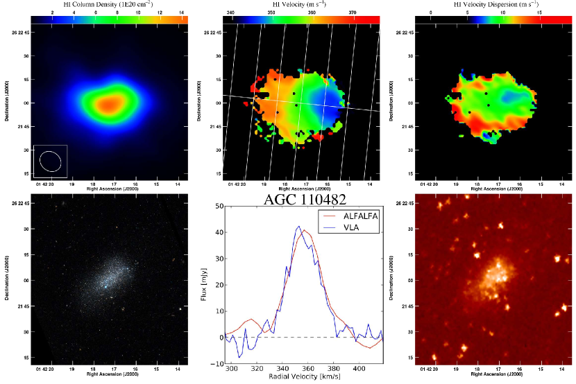
Figure 1.— The gaseous and stellar components of the SHIELD galaxy AGC 110482. Upper left: moment zero image generated from the naturally weighted image cube, manually blanked using the method described in Paper I, with the synthesized beam overlaid; the scale bar shows column density in units of 10²⁰ cm^-2. Upper middle: intensity-weighted velocity field, produced by fitting a single Gaussian function and blanking at the 10²⁰ atoms cm^-2 level from the moment zero image; the scale bar shows velocity in units of km s^-1. The singly-oriented white line represents the major axis position angle used to produce the top panel of Figure 14. The seven perpendicular white lines indicate the minor axis slices used to produce the bottom panels of Figure 14. The intersection of the central minor axis slice line with the major axis slice line is centered at the determined dynamical center of the galaxy. Upper right: velocity dispersion image, produced by fitting a single Gaussian function and blanking at the 10²⁰ atoms cm^-2 level from the moment zero image; the scale bar shows velocity dispersion in units of km s^-1. Lower left: three-color HST image of AGC 110482, as presented in McQuinn et al. (2014). Lower middle: global HI spectra using the VLA data (blue) and using the ALFALFA data (red). Lower right: Spitzer 4.5 µm image of AGC 110482.

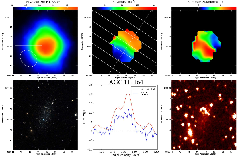
Figure 2.— Same as Figure 1, for AGC 111164

.

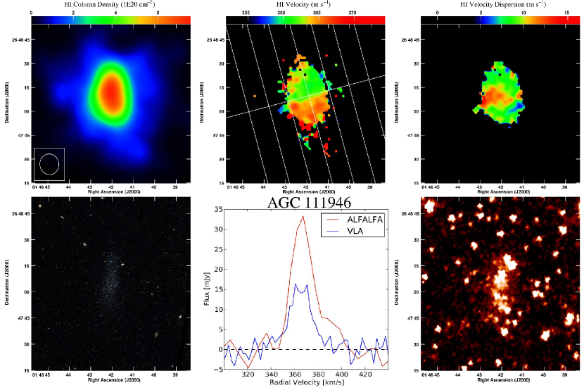
Figure 3.— Same as Figure 1, for AGC 111946.

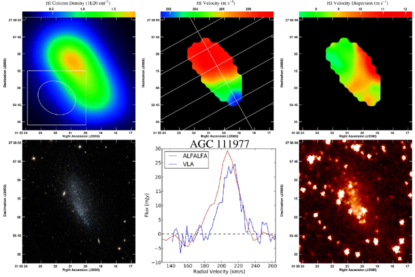
Figure 4.— Same as Figure 1, for AGC 111977.

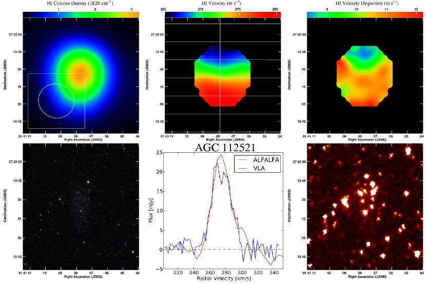
Figure 5.— Same as Figure 1, for AGC 112521.

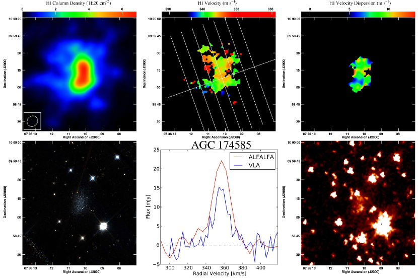
Figure 6.— Same as Figure 1, for AGC 174585.

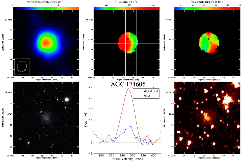
Figure 7.— Same as Figure 1, for AGC 174605.

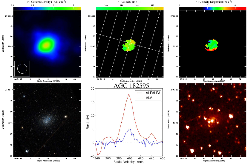
Figure 8.— Same as Figure 1, for AGC 182595.

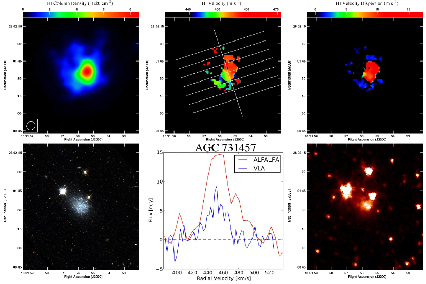
Figure 9.— Same as Figure 1, for AGC 731457.

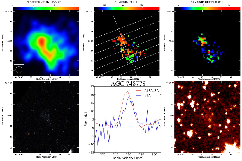
Figure 10.— Same as Figure 1, for AGC 748778.

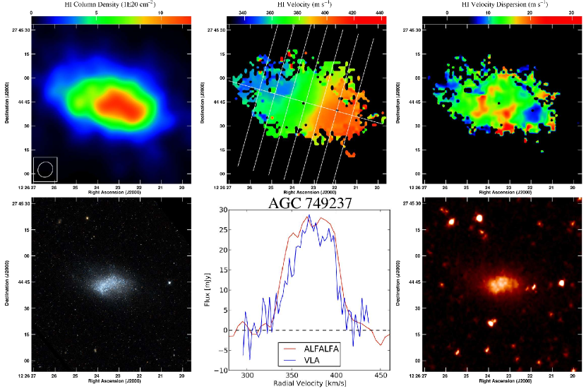
Figure 11.— Same as Figure 1, for AGC 749237.

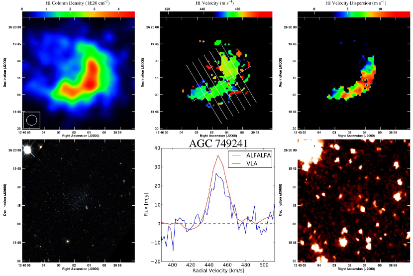
Figure 12.— Same as Figure 1, for AGC 749241.

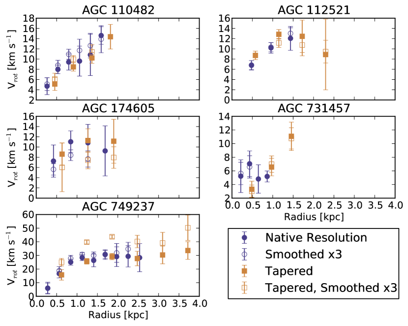
Figure 13.— Rotation curves of five SHIELD galaxies, as labeled; all results were obtained using the GIPSY task rotcur. The filled purple circles correspond to rotation velocities derived from velocity fields created with the full spatial and spectral resolution cubes; the filled gold squares correspond to rotation velocities derived from tapered cubes at full spectral resolution. The open purple circles signify full spatial resolution with velocity resolution decreased by a factor of three; the open gold squares show tapered data that have been likewise smoothed.

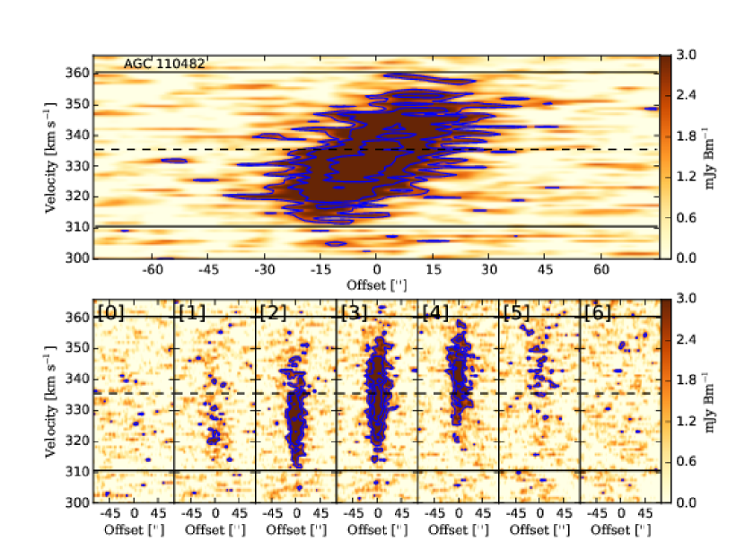
Figure 14.— Spatially resolved P-V diagrams across the major and minor axes of AGC 110482. The upper panel shows the slice taken across what was identified as the “major axis” of rotation (see Table 2) and that passes through the kinematic center. The lower panels show minor axis P-V cuts, spaced evenly by one beam width along the major axis; the central panel intersects the major axis slice at the dynamical center position. The slices used to generate these P-V maps are overlaid on the upper middle panel of Figure 1.

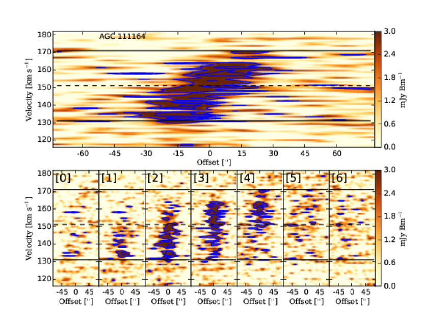
Figure 15.— Spatially resolved P-V diagrams across the major and minor axes of AGC 111164. The upper panel shows the slice taken across what was identified as the “major axis” of rotation (see Table 2) and that passes through the kinematic center. The lower panels show minor axis P-V cuts, spaced evenly by one beam width along the major axis; the central panel intersects the major axis slice at the dynamical center position. The slices used to generate these P-V maps are overlaid on the upper middle panel of Figure 2.

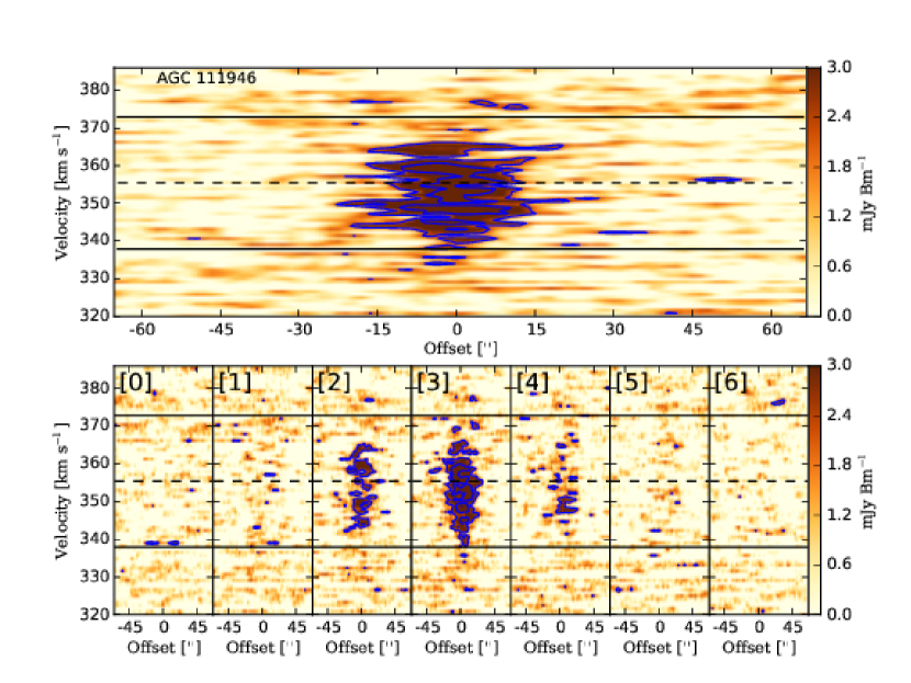
Figure 16.— Spatially resolved P-V diagrams across the major and minor axes of AGC 111946. The upper panel shows the slice taken across what was identified as the “major axis” of rotation (see Table 2) and that passes through the kinematic center. The major axis was defined to pass through the largest rotation gradient of the source, in spite of the $\sim$370km s^-1 outlying points to the northwest. The lower panels show minor axis P-V cuts, spaced evenly by one beam width along the major axis; the central panel intersects the major axis slice at the dynamical center position. The slices used to generate these P-V maps are overlaid on the upper middle panel of Figure 3.

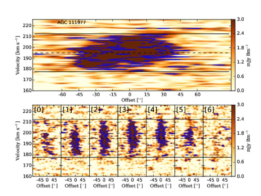
Figure 17.— Spatially resolved P-V diagrams across the major and minor axes of AGC 111977. The upper panel shows the slice taken across what was identified as the “major axis” of rotation (see Table 2) and that passes through the kinematic center. The lower panels show minor axis P-V cuts, spaced evenly by one beam width along the major axis; the central panel intersects the major axis slice at the dynamical center position. The slices used to generate these P-V maps are overlaid on the upper middle panel of Figure 4.

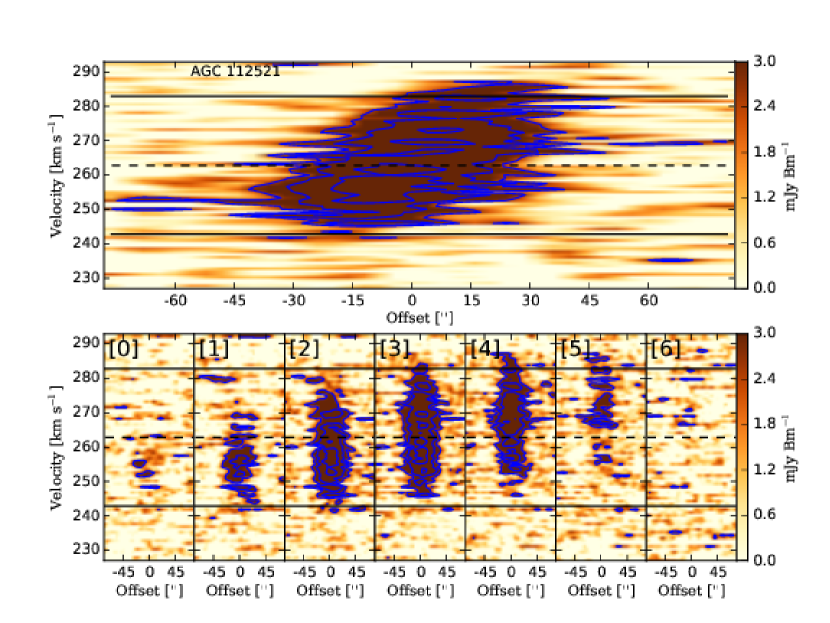
Figure 18.— Spatially resolved P-V diagrams across the major and minor axes of AGC 112521. The upper panel shows the slice taken across what was identified as the “major axis” of rotation (see Table 2) and that passes through the kinematic center. The lower panels show minor axis P-V cuts, spaced evenly by one beam width along the major axis; the central panel intersects the major axis slice at the dynamical center position. The slices used to generate these P-V maps are overlaid on the upper middle panel of Figure 5.

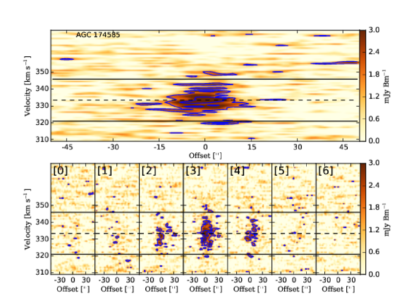
Figure 19.— Spatially resolved P-V diagrams across the major and minor axes of AGC 174585. The upper panel shows the slice taken across what was identified as the “major axis” of rotation (see Table 2) and that passes through the kinematic center. The lower panels show minor axis P-V cuts, spaced evenly by one beam width along the major axis; the central panel intersects the major axis slice at the dynamical center position. The slices used to generate these P-V maps are overlaid on the upper middle panel of Figure 6. Note that the major axis of AGC 174585 could be defined in two directions. There is an apparent rotation gradient across the southern lobe of the galaxy, but higher sensitivity images (the naturally-weighted data cube) appear to reveal stronger emission with higher velocity to the northwest, so the PV slice major axis was defined to trace through both lobes instead of across the bottom one for a few pixels of faint slow gas. Either low surface brightness gas- unresolved at high angular resolution- and the high surface brightness gas detected in our highest resolution maps have different rotation axes, or there is no preferential axis of rotation in this source.

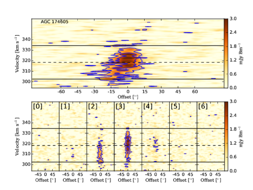
Figure 20.— Spatially resolved P-V diagrams across the major and minor axes of AGC 174605. The upper panel shows the slice taken across what was identified as the “major axis” of rotation (see Table 2) and that passes through the kinematic center. The lower panels show minor axis P-V cuts, spaced evenly by one beam width along the major axis; the central panel intersects the major axis slice at the dynamical center position. The slices used to generate these P-V maps are overlaid on the upper middle panel of Figure 7.

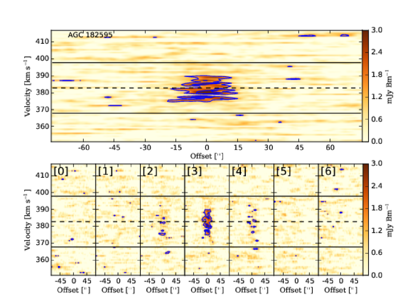
Figure 21.— Spatially resolved P-V diagrams across the major and minor axes of AGC 182595. The upper panel shows the slice taken across what was identified as the “major axis” of rotation (see Table 2) and that passes through the kinematic center. The lower panels show minor axis P-V cuts, spaced evenly by one beam width along the major axis; the central panel intersects the major axis slice at the dynamical center position. The slices used to generate these P-V maps are overlaid on the upper middle panel of Figure 8. Note that AGC 182595 is a source whose P-V diagrams appear to indicate no ordered rotation: the position angle of the P-V slice in this case has practically no effect on the resulting maps, and it was chosen such that by eye the radial offset (in position space) was maximized. Since the velocity ranges of the P-V maps were practically identical for all values of position angle, a few pixels’ change in radial offset was taken as a proxy for highest dispersive motion, the closest we could come to defining a “major” axis of rotation for this galaxy.

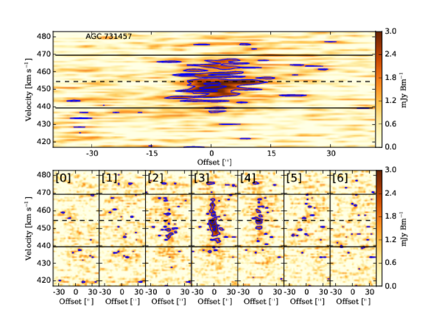
Figure 22.— Spatially resolved P-V diagrams across the major and minor axes of AGC 731457. The upper panel shows the slice taken across what was identified as the “major axis” of rotation (see Table 2) and that passes through the kinematic center. The lower panels show minor axis P-V cuts, spaced evenly by one beam width along the major axis; the central panel intersects the major axis slice at the dynamical center position. The slices used to generate these P-V maps are overlaid on the upper middle panel of Figure 9.

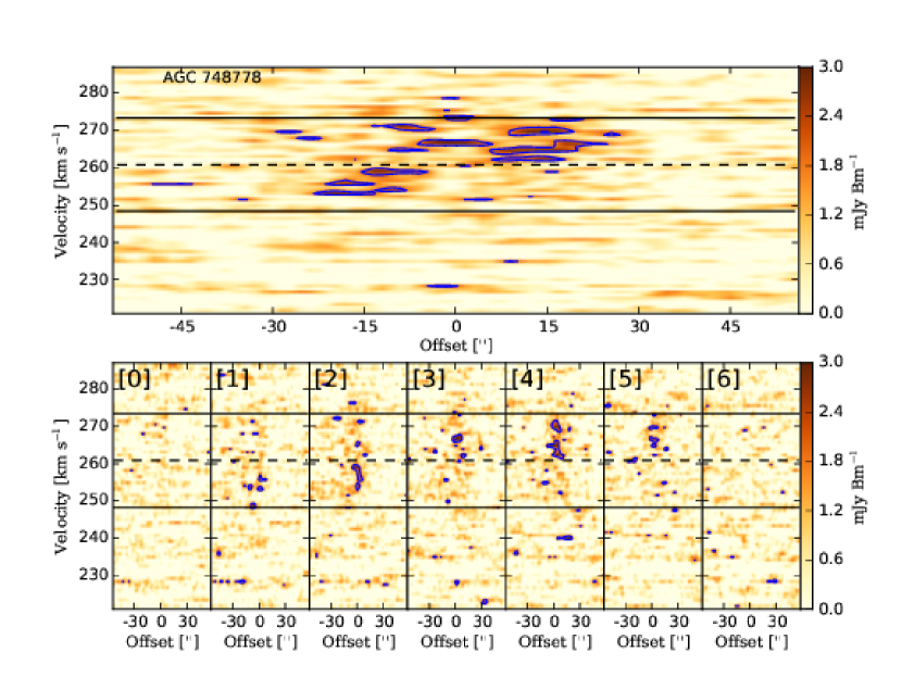
Figure 23.— Spatially resolved P-V diagrams across the major and minor axes of AGC 748778. The upper panel shows the slice taken across what was identified as the “major axis” of rotation (see Table 2) and that passes through the kinematic center. The lower panels show minor axis P-V cuts, spaced evenly by one beam width along the major axis; the central panel intersects the major axis slice at the dynamical center position. The slices used to generate these P-V maps are overlaid on the upper middle panel of Figure 10. Note that at the angular resolution of these data, the velocity structure that we detect in AGC 748778 is attributable to only the parcels of neutral gas with highest surface brightness. Therefore, the position angle used to define a “major” axis was determined to be across the region of highest significant emission in the moment 0 map, which also happens to correspond to what looks like a weak velocity gradient from the southeast to the northwest.

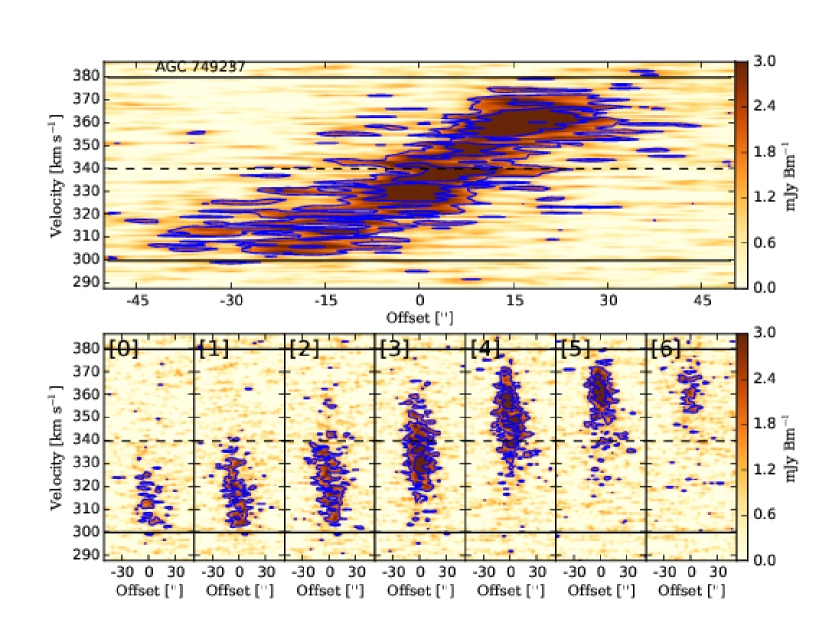
Figure 24.— Spatially resolved P-V diagrams across the major and minor axes of AGC 749237. The upper panel shows the slice taken across what was identified as the “major axis” of rotation (see Table 2) and that passes through the kinematic center. The lower panels show minor axis P-V cuts, spaced evenly by one beam width along the major axis; the central panel intersects the major axis slice at the dynamical center position. The slices used to generate these P-V maps are overlaid on the upper middle panel of Figure 11.

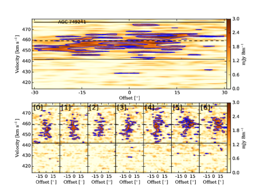
Figure 25.— Spatially resolved P-V diagrams across the major and minor axes of AGC 749241. The upper panel shows the slice taken across what was identified as the “major axis” of rotation (see Table 2) and that passes through the kinematic center. The lower panels show minor axis P-V cuts, spaced evenly by one beam width along the major axis; the central panel intersects the major axis slice at the dynamical center position. The slices used to generate these P-V maps are overlaid on the upper middle panel of 12. Note that the highly irregular “crescent-shaped” distribution of neutral gas in this source makes the selection of an unambiguous position angle extremely subjective. It was chosen to match the arcing structure of the highest column density gas, which also shows a very weak gradient from outer southwest to the inner northeast edges.

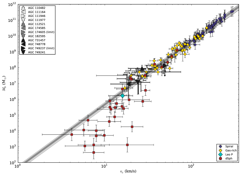
Figure 26.— The fundamental plane of the mass-velocity scaling relation, commonly referred to as the Baryonic Tully-Fisher relation (BTFR). The smaller points correspond to data from the literature (see the compilation by McGaugh (2012) and references therein). The purple circles correspond to spiral galaxies with available HI line-width data whose baryonic mass is dominated by the stellar component. The gold diamonds represent the less massive gas-rich galaxies used to calibrate the model, and the red squares represent spheroidal dwarf galaxies with no detectable HI. The larger cyan diamond represents Leo P, the slowest rotating and lowest-mass galaxy known to still be relatively rich with interstellar gas (Bernstein-Cooper et al. 2014). The gray bars represent 1 and 3 $\sigma$ deviations from a fit of the BTFR to the gas-rich galaxy sample. The large greyscale triangles represent the SHIELD galaxies. The SHIELD galaxy sample is fit significantly by the model; ten galaxies agree within model uncertainty of 1 $\sigma$ and all 12 agree within 3 $\sigma$ model uncertainty.

Appendix A Channel Maps of the SHIELD Galaxies

We present channel maps for all 12 SHIELD galaxies. These data cubes were used to produce the moment images shown along the top row in Figures 1 through 12.

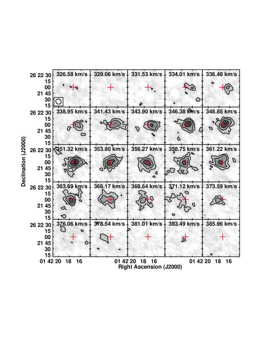
Figure 27.— Channel map of the naturally-weighted, Hanning smoothed (by 3 channels) data cube for AGC 110482. The beam size is shown in the top left panel; the red crosshair is located at the identified dynamical center (see Table 1). The contours proceed in doubling intervals above 1$\times$10²⁰ atoms cm^-2.

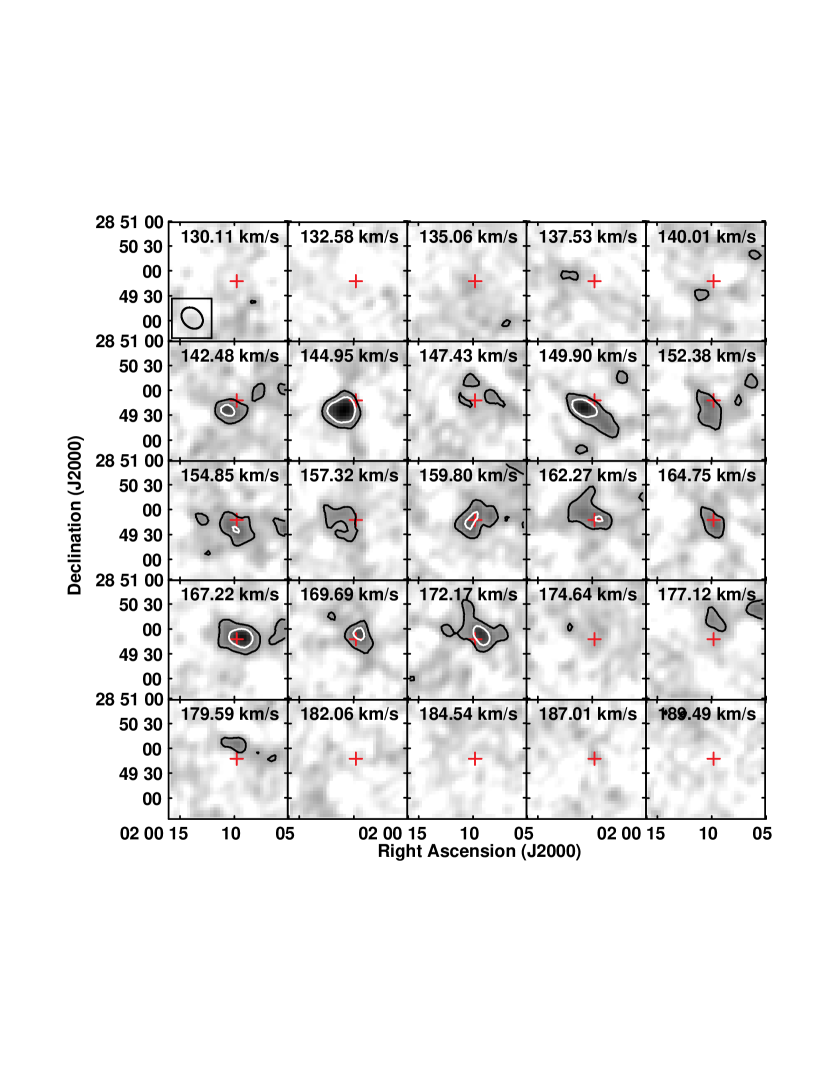
Figure 28.— Same as Figure 33, for AGC 111164.

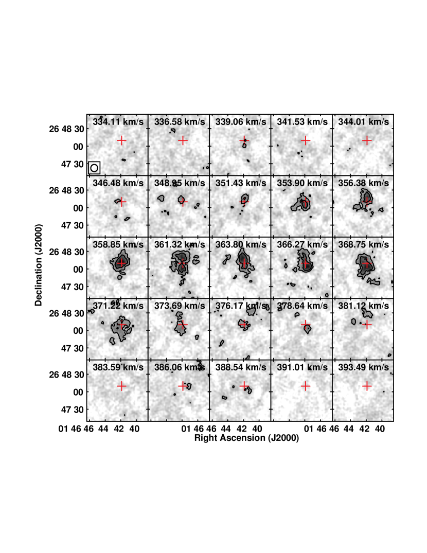
Figure 29.— Same as Figure 33, for AGC 111946.

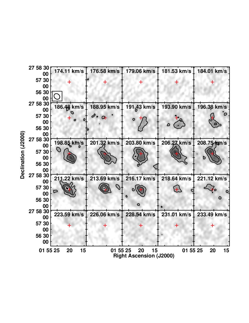
Figure 30.— Same as Figure 33, for AGC 111977.

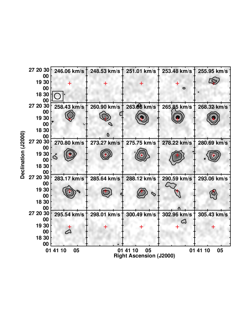
Figure 31.— Same as Figure 33, for AGC 112521.

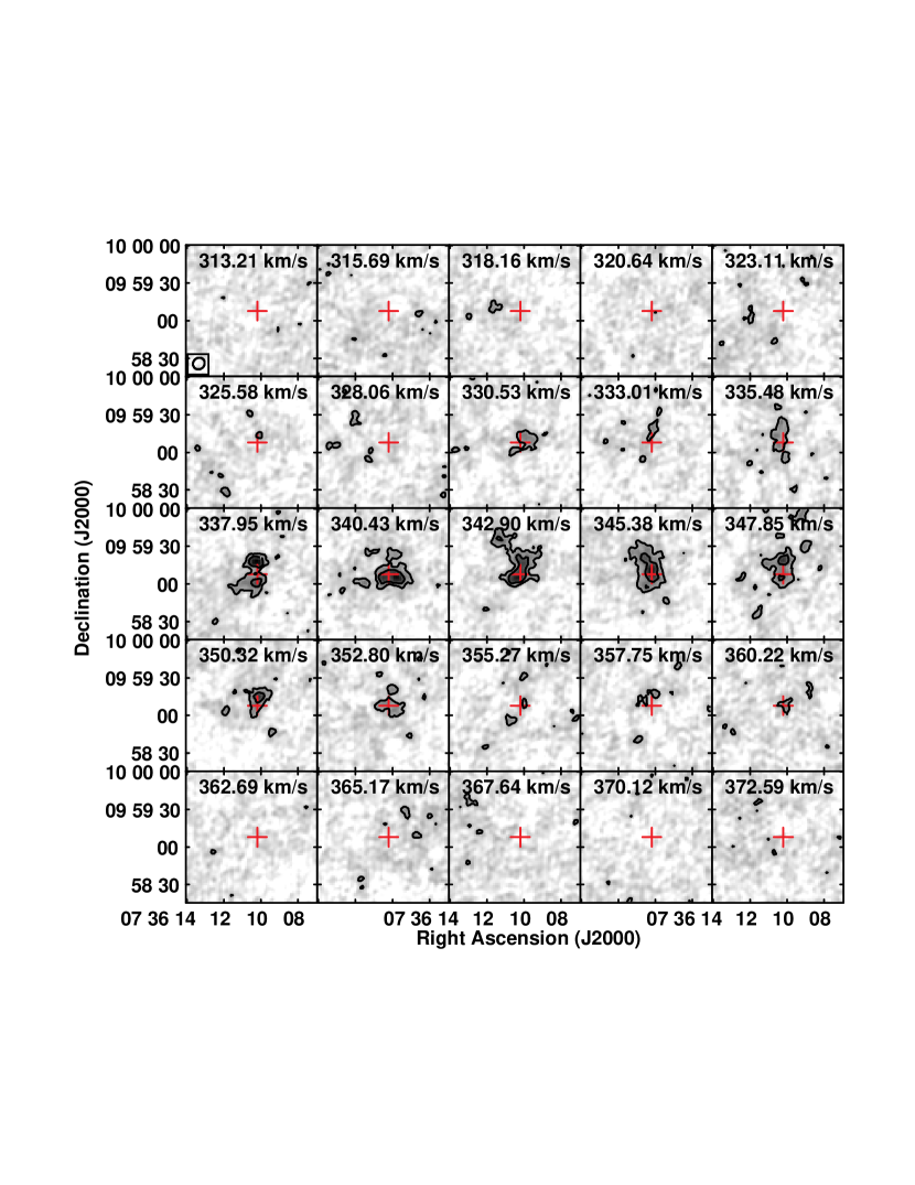
Figure 32.— Same as Figure 33, for AGC 174585.

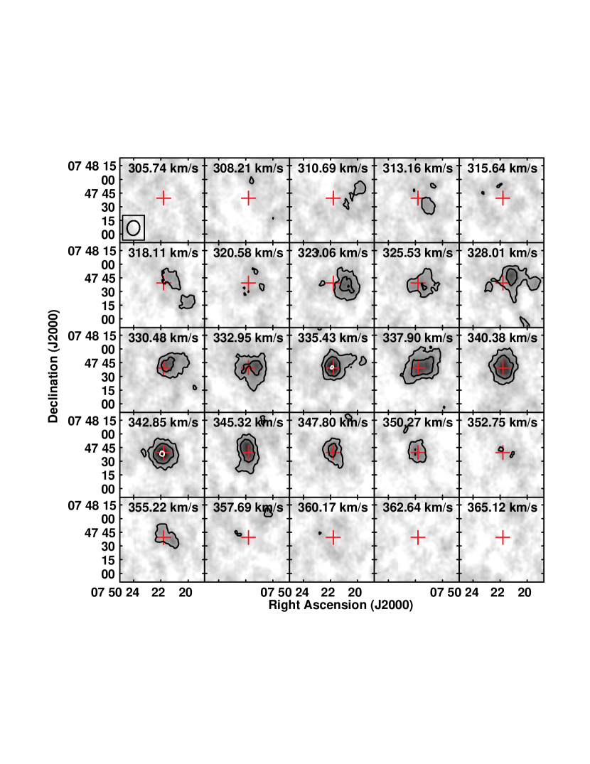
Figure 33.— Same as Figure 33, for AGC 174605.

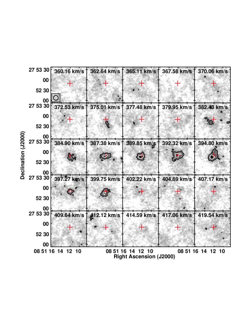
Figure 34.— Same as Figure 33, for AGC 182595.

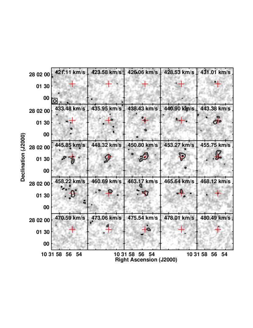
Figure 35.— Same as Figure 33, for AGC 731457.

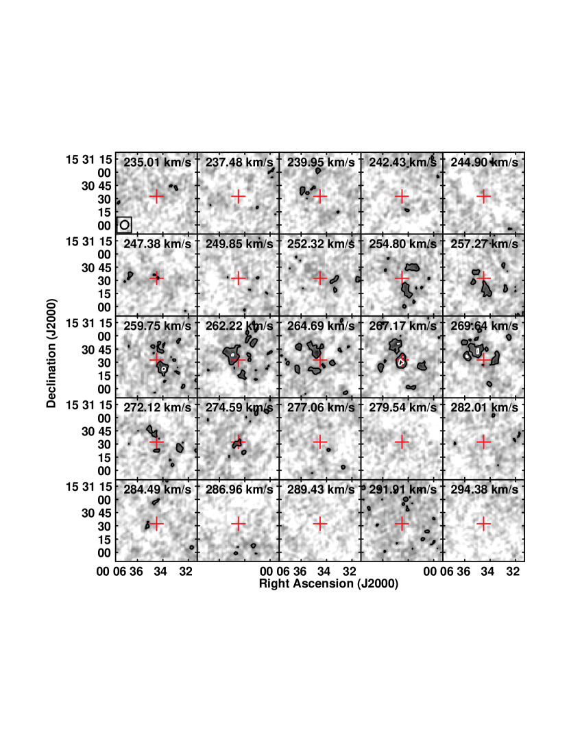
Figure 36.— Same as Figure 33, for AGC 748778.

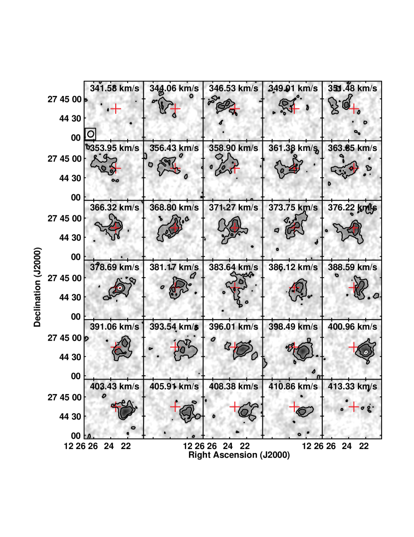
Figure 37.— Same as Figure 33, for AGC 749237.

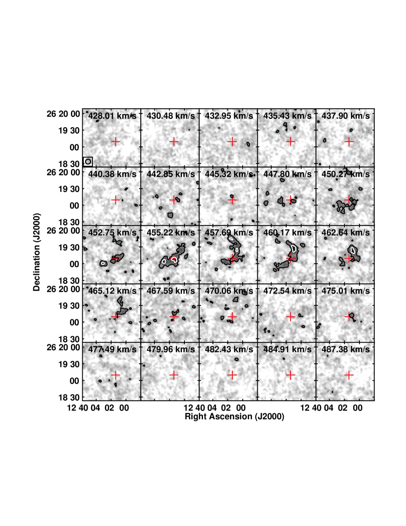
Figure 38.— Same as Figure 33, for AGC 749241.

References

- Adams et al. (2013) Adams, E. A. K., Giovanelli, R., & Haynes, M. P. 2013, ApJ, 768, 77
- Adams et al. (2014) Adams, J. J., Simon, J. D., Fabricius, M. H., et al. 2014, ApJ, 789, 63
- Astropy Collaboration et al. (2013) Astropy Collaboration, Robitaille, T. P., Tollerud, E. J., et al. 2013, A&A, 558, A33
- Begum et al. (2008) Begum, A., Chengalur, J. N., Karachentsev, I. D., Sharina, M. E., & Kaisin, S. S. 2008, MNRAS, 386, 1667
- Bernstein-Cooper et al. (2014) Bernstein-Cooper, E. Z., Cannon, J. M., Elson, E. C., et al. 2014, AJ, 148, 35
- Boylan-Kolchin et al. (2011) Boylan-Kolchin, M., Bullock, J. S., & Kaplinghat, M. 2011, MNRAS, 415, L40
- (7) Briggs, D. S. 1995, Bulletin of the American Astronomical Society, 27, #112.02
- Cannon et al. (2011a) Cannon, J. M., Most, H. P., Skillman, E. D., et al. 2011, ApJ, 735, 35
- Cannon et al. (2012) Cannon, J. M., Bernstein-Cooper, E. Z., Cave, I. M., et al. 2012, AJ, 144, 82
- Cannon et al. (2013) Cannon, J. M., Marshall, M., Cave, I., et al. 2013, American Astronomical Society Meeting Abstracts #221, 221, 352.04
- Cannon et al. (2015) Cannon, J. M., Martinkus, C. P., Leisman, L., et al. 2015, AJ, 149, 72
- Carignan (2015) Carignan, C. 2015, IAU General Assembly, 23, 1455
- Corbelli & Schneider (1997) Corbelli, E., & Schneider, S. E. 1997, ApJ, 479, 244
- Davis et al. (2013) Davis, T. A., Alatalo, K., Bureau, M., et al. 2013, MNRAS, 429, 534
- de Blok (2010) de Blok, W. J. G. 2010, Advances in Astronomy, 2010, 789293
- Di Cintio et al. (2014) Di Cintio, A., Brook, C. B., Dutton, A. A., et al. 2014, MNRAS, 441, 2986
- Di Teodoro & Fraternali (2015) Di Teodoro, E. M., & Fraternali, F. 2015, MNRAS, 451, 3021
- Elson et al. (2013) Elson, E. C., de Blok, W. J. G., & Kraan-Korteweg, R. C. 2013, MNRAS, 429, 2550
- Elson (2014) Elson, E. C. 2014, MNRAS, 437, 3736
- Eskew et al. (2012) Eskew, M., Zaritsky, D., & Meidt, S. 2012, AJ, 143, 139
- Ewen & Purcell (1951) Ewen, H. I., & Purcell, E. M. 1951, Nature, 168, 356
- Fraternali et al. (2002) Fraternali, F., van Moorsel, G., Sancisi, R., & Oosterloo, T. 2002, AJ, 123, 3124
- Frusciante et al. (2012) Frusciante, N., Salucci, P., Vernieri, D., Cannon, J. M., & Elson, E. C. 2012, MNRAS, 426, 751
- Garrison-Kimmel et al. (2014) Garrison-Kimmel, S., Boylan-Kolchin, M., Bullock, J. S., & Kirby, E. N. 2014, MNRAS, 444, 222
- Giovanelli et al. (2005) Giovanelli, R., Haynes, M. P., Kent, B. R., et al. 2005, AJ, 130, 2598
- Giovanelli et al. (2013) Giovanelli, R., Haynes, M. P., Adams, E. A. K., et al. 2013, AJ, 146, 15
- Gooch (1996) Gooch, R. 1996, Astronomical Data Analysis Software and Systems V, 101, 80
- Gordon et al. (2016) Gordon, A. J. R., Cannon, J. M., Adams, E. A., & SHIELD II Team 2016, American Astronomical Society Meeting Abstracts, 227, 136.04
- Hagen et al. (2014) Hagen, C., Cannon, J. M., Cave, I., et al. 2014, American Astronomical Society Meeting Abstracts #223, 223, #355.16
- Haurberg et al. (2015) Haurberg, N. C., Salzer, J. J., Cannon, J. M., & Marshall, M. V. 2015, ApJ, 800, 121
- Hoffman et al. (1996) Hoffman, G. L., Salpeter, E. E., Farhat, B., et al. 1996, ApJS, 105, 269
- Huang et al. (2012a) Huang, S., Haynes, M. P., Giovanelli, R., & Brinchmann, J. 2012, ApJ, 756, 113
- Huang et al. (2012b) Huang, S., Haynes, M. P., Giovanelli, R., et al. 2012, AJ, 143, 133
- Hunter et al. (2012) Hunter, D. A., Ficut-Vicas, D., Ashley, T., et al. 2012, AJ, 144, 134
- Janowiecki et al. (2015) Janowiecki, S., Leisman, L., Józsa, G., et al. 2015, ApJ, 801, 96
- Jorsater & van Moorsel (1995) Jorsater, S., & van Moorsel, G. A. 1995, AJ, 110, 2037
- Józsa et al. (2007) Józsa, G. I. G., Kenn, F., Klein, U., & Oosterloo, T. A. 2007, A&A, 468, 731
- Kauffmann et al. (1993) Kauffmann, G., White, S. D. M., & Guiderdoni, B. 1993, MNRAS, 264, 201
- Kerr et al. (1954) Kerr, F. J., Hindman, J. F., & Robinson, B. J. 1954, Australian Journal of Physics, 7, 297
- Kirby et al. (2012) Kirby, E. M., Koribalski, B., Jerjen, H., & López-Sánchez, Á. 2012, MNRAS, 420, 2924
- Klypin et al. (2015) Klypin, A., Karachentsev, I., Makarov, D., & Nasonova, O. 2015, MNRAS, 454, 1798
- Klypin et al. (1999) Klypin, A., Kravtsov, A. V., Valenzuela, O., & Prada, F. 1999, ApJ, 522, 82
- Lee et al. (2016) Lee, E., Cannon, J. M., McNichols, A., Teich, Y., & SHIELD II Team 2016, American Astronomical Society Meeting Abstracts, 227, 136.07
- Lelli et al. (2016) Lelli, F., McGaugh, S. S., & Schombert, J. M. 2016, ApJ, 816, L14
- Marshall (2013) Marshall, M. 2013, American Astronomical Society Meeting Abstracts #221, 221, 352.05
- Masters (2005) Masters, K. L. 2005, Ph.D. Thesis,
- Mateo (1998) Mateo, M. L. 1998, ARA&A, 36, 435
- McGaugh et al. (2000) McGaugh, S. S., Schombert, J. M., Bothun, G. D., & de Blok, W. J. G. 2000, ApJ, 533, L9
- McGaugh (2012) McGaugh, S. S. 2012, AJ, 143, 40
- McMullin et al. (2007) McMullin, J. P., Waters, B., Schiebel, D., Young, W., & Golap, K. 2007, Astronomical Data Analysis Software and Systems XVI, 376, 127
- McNichols et al. (2015) McNichols, A., Teich, Y., Cannon, J. M., et al. 2015, American Astronomical Society Meeting Abstracts, 225, #248.20
- McQuinn et al. (2014) McQuinn, K. B. W., Cannon, J. M., Dolphin, A. E., et al. 2014, ApJ, 785, 3
- McQuinn et al. (2015a) McQuinn, K. B. W., Cannon, J. M., Dolphin, A. E., et al. 2015a, ApJ, 802, 66
- McQuinn et al. (2015b) McQuinn, K. B. W., Skillman, E. D., Dolphin, A. E., et al. 2015b, ApJ, 812, 156
- Meyer et al. (2004) Meyer, M. J., Zwaan, M. A., Webster, R. L., et al. 2004, MNRAS, 350, 1195
- Moore et al. (1999) Moore, B., Ghigna, S., Governato, F., et al. 1999, ApJ, 524, L19
- Navarro et al. (1997) Navarro, J. F., Frenk, C. S., & White, S. D. M. 1997, ApJ, 490, 493
- Oh et al. (2011) Oh, S.-H., de Blok, W. J. G., Brinks, E., Walter, F., & Kennicutt, R. C., Jr. 2011, AJ, 141, 193
- Oh et al. (2015) Oh, S.-H., Hunter, D. A., Brinks, E., et al. 2015, AJ, 149, 180
- Ott et al. (2012) Ott, J., Stilp, A. M., Warren, S. R., et al. 2012, AJ, 144, 123
- Papastergis et al. (2015) Papastergis, E., Giovanelli, R., Haynes, M. P., & Shankar, F. 2015, A&A, 574, A113
- Papastergis et al. (2016) Papastergis, E., Adams, E.A.K., & van der Hulst, J.M. 2016, A&A, submitted (ArXiV/1602.09087)
- Perley & Butler (2013) Perley, R. A., & Butler, B. J. 2013, ApJS, 204, 19
- Rhode et al. (2013) Rhode, K. L., Salzer, J. J., Haurberg, N. C., et al. 2013, AJ, 145, 149
- Robles et al. (2015) Robles, V. H., Lora, V., Matos, T., & Sánchez-Salcedo, F. J. 2015, ApJ, 810, 99
- Rogstad et al. (1974) Rogstad, D. H., Lockhart, I. A., & Wright, M. C. H. 1974, ApJ, 193, 309
- Rubio et al. (2015) Rubio, M., Elmegreen, B. G., Hunter, D. A., et al. 2015, Nature, 525, 218
- Salak et al. (2016) Salak, D., Nakai, N., Hatakeyama, T., & Miyamoto, Y. 2016, arXiv:1603.05881
- Schmidt et al. (2014) Schmidt, P., Józsa, G. I. G., Gentile, G., et al. 2014, A&A, 561, A28
- Schwab (1984) Schwab, F. R. 1984, AJ, 89, 1076
- Spekkens et al. (2005) Spekkens, K., Giovanelli, R., & Haynes, M. P. 2005, AJ, 129, 2119
- Stark et al. (2009) Stark, D. V., McGaugh, S. S., & Swaters, R. A. 2009, AJ, 138, 392
- Staveley-Smith et al. (1992) Staveley-Smith, L., Davies, R. D., & Kinman, T. D. 1992, MNRAS, 258, 334
- Stevens et al. (2016) Stevens, K., Cannon, J. M., McNichols, A., et al. 2016, American Astronomical Society Meeting Abstracts, 227, 136.05
- Stilp et al. (2013) Stilp, A. M., Dalcanton, J. J., Skillman, E., et al. 2013, ApJ, 773, 88
- Swaters et al. (2002) Swaters, R. A., van Albada, T. S., van der Hulst, J. M., & Sancisi, R. 2002, A&A, 390, 829
- Tamburro et al. (2009) Tamburro, D., Rix, H.-W., Leroy, A. K., et al. 2009, AJ, 137, 4424
- Teich et al. (2016) Teich, Y. G., Cannon, J. M., McNichols, A. T., et al. 2016, ApJ, submitted
- Thomann et al. (2012) Thomann, C., Cannon, J. M., Elson, E. C., et al. 2012, American Astronomical Society Meeting Abstracts #219, 219, #244.03
- Trachternach et al. (2009) Trachternach, C., de Blok, W. J. G., McGaugh, S. S., van der Hulst, J. M., & Dettmar, R.-J. 2009, A&A, 505, 577
- Tully & Fisher (1977) Tully, R. B., & Fisher, J. R. 1977, A&A, 54, 661
- van der Hulst et al. (1992) van der Hulst, J. M., Terlouw, J. P., Begeman, K. G., Zwitser, W., & Roelfsema, P. R. 1992, Astronomical Data Analysis Software and Systems I, 25, 131
- Verbeke et al. (2015) Verbeke, R., Vandenbroucke, B., De Rijcke, S., & Koleva, M. 2015, IAU General Assembly, 22, 2232938
- Walker & Peñarrubia (2011) Walker, M. G., & Peñarrubia, J. 2011, ApJ, 742, 20
- Warren et al. (2015) Warren, S. R., Molter, E., Cannon, J. M., et al. 2015, ApJ, 814, 30
- Wiegert et al. (2006) Wiegert, T., English, J., & Fiege, J. 2006, Bulletin of the American Astronomical Society, 38, 96
- Wiegert (2011) Wiegert, T. B. V. 2011, Ph.D. Thesis
- Wiegert & English (2014) Wiegert, T., & English, J. 2014, New Astronomy, 26, 40
- Wendt et al. (2008) Wendt, H., Orchiston, W., & Slee, B. 2008, Journal of Astronomical History and Heritage, 11, 185