SHIELD: Comparing Gas and Star Formation in Low Mass Galaxies

Abstract

We analyze the relationships between atomic, neutral hydrogen (H I) and star formation (SF) in the 12 low-mass SHIELD galaxies. We compare high spectral ($\sim$0.82 km s^-1 ch^-1) and spatial resolution (physical resolutions of 170 pc – 700 pc) H I imaging from the VLA with H$\alpha$ and far-ultraviolet imaging. We quantify the degree of co-spatiality between star forming regions and regions of high H I column densities. We calculate the global star formation efficiencies (SFE, $\Sigma_{\rm SFR}$ / $\Sigma_{\rm H~{}{\sc I}}$), and examine the relationships among the SFE and H I mass, H I column density, and star formation rate (SFR). The systems are consuming their cold neutral gas on timescales of order a few Gyr. While we derive an index for the Kennicutt-Schmidt relation of $N$ $\approx$ 0.68$\pm$0.04 for the SHIELD sample as a whole, the values of $N$ vary considerably from system to system. By supplementing SHIELD results with those from other surveys, we find that HI mass and UV-based SFR are strongly correlated over five orders of magnitude. Identification of patterns within the SHIELD sample allows us to bin the galaxies into three general categories: 1) mainly co-spatial H I and SF regions, found in systems with highest peak H I column densities and highest total H I masses; 2) moderately correlated H I and SF regions, found in systems with moderate H I column densities; and 3) obvious offsets between H I and SF peaks, found in systems with the lowest total H I masses. SF in these galaxies is dominated by stochasticity and random fluctuations in their ISM.

1. Introduction

1.1. Stars and Gas in Galaxies

The conversion of gas into stars is one of the most fundamental processes in astronomy. Yet, despite decades of effort, a simple prescription of star formation (SF) that successfully describes all observations of galaxies across a range of halo masses has remained elusive. In broad terms, more massive star-forming galaxies will have larger gas reservoirs (both atomic and molecular) and higher global star formation rates (SFR) than less massive systems (see, e.g., Kennicutt, 1998a). However, the gas mass fractions in star forming galaxies tend to increase with decreasing mass (e.g., Fisher & Tully, 1975).

Empirical correlations between gas properties and various tracers of instantaneous (using H$\alpha$ emission, with a characteristic timescale of $<$$\sim$ 10 Myr) or ongoing (using FUV emission, with a characteristic timescale of $<$$\sim$ 100 Myr) SF have been numerous in the literature. The most common parameterization relates a SFR surface density to a gas surface density:

$$\Sigma_{\rm SFR}\propto(\Sigma_{\rm gas})^{N}$$ (1)

with the SFR surface density ($\Sigma_{\rm SFR}$) in units of M_⊙ yr^-1 kpc^-2, the gas surface density ($\Sigma_{\rm gas}$) in units of M_⊙ pc^-2, and $N$ being a positive number. Schmidt (1959) found that $N\approx 2$, and similar indices have been derived numerous times over the last half-century (see Elmegreen 2011 for a recent review). For example, Kennicutt (1998b) found $N=$ 1.4 $\pm$ 0.15 for 61 large spiral galaxies when relating the H$\alpha$-based SFR to the total gas surface density (via both H I and CO observations, where the CO is used as a tracer for molecular gas).

In a study of this relation on sub-kpc scales, Bigiel et al. (2008) found that the relationship between the total gas surface density and the SFR surface density varied dramatically among and within individual spiral galaxies, and that most of the sample showed little or no correlation between $\Sigma_{\rm H~{}{\sc I}}$ and $\Sigma_{\rm SFR}$. In an associated paper, Leroy et al. (2008) found a molecular Schmidt power-law slope of $N=1.0\pm 0.2$ in 18 nearby spiral galaxies; similarly, Momose et al. (2013) found $N=$ 1.3 - 1.8 for 10 nearby spiral galaxies. In a subsequent study, Bigiel et al. (2010) find no clear evidence for SF thresholds and emphasize that it may not be realistic to expect them.

Molecular gas in low mass galaxies remains largely undetectable via traditional CO tracers, thus studying the relationship between atomic gas and SF is especially important in these metal-poor low-mass systems (e.g., Bolatto et al., 2013). In fact, very few detections of CO gas exist at metallicities less than $\sim$10% Z_⊙, even in systems that are actively forming stars (see, e.g., Taylor et al. 1998, Schruba et al. 2012, Warren et al. 2015). For low mass galaxies, this implies that studying the relationship between $\Sigma_{\rm SFR}$ and $\Sigma_{\rm gas}$ as a function of galaxy mass is necessarily constrained to only the atomic gas component.

It is thus interesting to note that a correlation between $\Sigma_{\rm H~{}{\sc I}}$ and $\Sigma_{\rm SFR}$ appears to hold in some galaxies and not in others. For example, Bigiel et al. (2008) find that $\Sigma_{\rm H~{}{\sc I}}$ and $\Sigma_{\rm SFR}$ are not related in individual spiral disks. This can be compared to the results in Skillman (1987), which show that 10²¹ cm^-2 (corresponding to 7.9 M_⊙ pc^-2 or 10.6 M_⊙ pc^-2 when accounting for helium) represents a requisite threshold H I surface density for massive SF. Similarly, Wyder et al. (2009) examined 19 low surface-brightness galaxies and found an apparent threshold in the H I gas surface density in the range 3 $-$ 10 M_⊙ pc^-2 below which very little SF (traced by H$\alpha$) is observed. Extending to even lower masses, Roychowdhury et al. (2009) and Roychowdhury et al. (2011) find that all H I gas in their galaxies with $\Sigma_{\rm H~{}{\sc I}}$ $\gtrsim$ 10 M_⊙ pc^-2 ($\approx$ 1.2$\times$10²¹ cm^-2) have associated SF, but there is no threshold below which SF is not observed (that is, SF is observed in regions with H I columns $<$ 10²¹ cm^-2). Most recently, Roychowdhury et al. (2014) found that the $\Sigma_{\rm H~{}{\sc I}}$ $-$ $\Sigma_{\rm SFR}$ relation for a set of dwarf irregular galaxies was nearly linear. Roychowdhury et al. (2015) find consistency across a range of scales (400pc and 1kpc) and galaxy types, including both low-mass galaxies and more massive spiral disks.

Based on the above results, it is not trivial to anticipate where in a galaxy one will observe ongoing SF - regardless of how massive that galaxy is. Knowledge of the H I properties alone is often insufficient to predict where in a given galaxy the conditions are ripe for SF. For example, Krumholz (2012) suggests that molecular gas is a better predictor of SF than the neutral ISM. We examine this issue from the H I perspective in Section 4.2.

In addition to the $\Sigma_{\rm gas}$ vs. $\Sigma_{\rm SFR}$ analysis, we also study the star formation efficiency (SFE), which is a useful metric when discussing where in a galaxy SF is occurring (Leroy et al., 2008). Several ways of describing the SFE exist, but for consistency with other surveys we use SFE = $\Sigma_{\rm SFR}/\Sigma_{\rm gas}$ with units of yr^-1. The SFE is more useful than SFR alone to identify where conditions are conducive to SF because it is normalized by the gas mass surface density. Thus, it quantifies the local physical properties in regions where the gas is being turned into stars efficiently: regions of elevated gas surface density which have no young stars associated with them are inefficient, while regions of elevated gas surface density that show co-spatiality with young stars are efficient. Conveniently, the inverse of the SFE is the gas depletion time, which is the time required for SF to consume the gas reservoir at the present-day SFR. For a sample of low-mass galaxies, Roychowdhury et al. (2014) found gas depletion timescales of $\sim$10¹⁰ yr, an order of magnitude lower than is estimated for the outer regions of large spiral galaxies (Bigiel et al., 2010). We calculate gas consumption times for our sample of galaxies in Section 4.2.

1.2. Low-Mass Galaxies from ALFALFA

The ALFALFA survey (Giovanelli et al., 2005) has produced one of the largest and most statistically useful catalogs of nearby, gas-rich galaxies to date. The final ALFALFA database will include source parameters for more than 30,000 systems. With the acquisition of data for ALFALFA now complete, a unique database exists to facilitate the study of fundamental galaxy properties across an unprecedented range of physical parameters. One particularly rich area of exploration that has been enabled by ALFALFA is a robustly-populated faint end of the H I mass function (Martin et al., 2010). Specifically, it is possible to identify a complete sample of gas-bearing, low-mass galaxies by matching the ALFALFA database to existing optical survey data.

As introduced in Cannon et al. (2011), the “Survey of H I in Extremely Low-mass Dwarfs” (hereafter, SHIELD) is a multi-wavelength, detailed study of the properties of ALFALFA-discovered or cataloged systems with extremely small H I mass reservoirs (see Section 2 for detailed discussion of the sample selection). Subsequent works have established the distances (McQuinn et al., 2014), the nebular abundances (Haurberg et al., 2015), and the qualities of SF based on spatially resolved Hubble Space Telescope (HST) imaging (McQuinn et al., 2015a). The primary goals of SHIELD are to 1) characterize the nature of SF in very low-mass galaxies and to 2) determine what fraction of the mass in these low-mass galaxies is baryonic. In this work, we undertake a comparative study of the H I gas and various tracers of recent SF in order to address goal #1. A companion paper by McNichols et al. (2016) explores the dynamical properties of our sample galaxies in order to address goal #2.

SHIELD is one of a number of recent H I surveys of dwarf galaxies using interferometric data. This list includes WHISP (The Westerbork H I Survey of Irregular and Spiral Galaxies; Swaters 2002), FIGGS (Faint Irregular Galaxies GMRT Survey; Begum et al. 2008), VLA-ANGST (Very Large Array Survey of ACS Nearby Galaxy Survey Treasury Galaxies; Ott et al. 2012), LITTLE-THINGS (Local Irregulars That Trace Luminosity Extremes in The H I Nearby Galaxy Survey; Hunter et al. 2012), and LVHIS (The Local Volume H I Survey; Kirby 2012). These studies have yielded valuable insights into a total of nearly two dozen systems with M${}_{\rm H~{}{\sc I}}$ $<$$\sim$ $10^{7}$ M_⊙. SHIELD adds to this relatively understudied region of parameter space by significantly increasing the number of sources with resolved H I imaging.

2. Galaxy Sample, Observations, and Data Handling

2.1. Sample Selection

SHIELD is a multi-wavelength survey of 12 low-mass galaxies in the Local Volume. Sample members were selected from the first $\sim$10% of the ALFALFA-detected galaxies on the basis of estimated H I mass (M${}_{\rm H~{}{\sc I}}$ $<$ 10^7.2, based on flow model distances using the prescription of Masters 2005). The W₅₀ condition (H I line width at 50% of peak $<$ 65 km s^-1, with no correction for inclination which would increase rotational velocity) discriminates against massive but H I-poor galaxies and identifies truly low-mass galaxies. Following the presentation of early SHIELD results in Cannon et al. (2011), the sources were observed with HST to derive their distances via the tip of the red giant branch (TRGB) method. The details are given in McQuinn et al. (2014); all sources moved to somewhat higher distances than the flow model predictions and so the H I masses of the systems are slightly increased. Even with the updated distances, all but one of the galaxies has M${}_{\rm H~{}{\sc I}}$ $<$ 10^7.3. The median distance, H I mass, and H I line width for the sample are 7.86 Mpc, 10^7.06 M_⊙, and 25 km s^-1, respectively. Table 1 provides a summary of physical characteristics of the SHIELD galaxies.

2.2. Data Products

2.2.1 Karl G. Janksy Very Large Array H I Data

The H I data for the survey were obtained using the Karl G. Janksy VLA in multiple array configurations for programs VLA/10B-187 (legacy code AC 990; P.I. Cannon) and VLA/13A-027 (legacy code AC 1115; P.I. Cannon). Our observational strategy (9, 4, and 2 hours of observation per source in the B, C, and D arrays of the VLA, respectively, with typical calibration overheads of 25%) achieves high spatial ($\sim$6″ synthesized beam at full resolution) and spectral resolution ($\sim$0.824 km s^-1 ch^-1), while retaining sensitivity to extended structure. The WIDAR correlator is used to provide a single 1 MHz sub-band with 2 polarization products and 256 channels each, covering 211 km s^-1 of frequency space at 3.906 kHz ch^-1, which is the setup for the B- and C-configuration observations. For the D-configuration observations, the frequency coverage was widened to 4 MHz (corresponding to 1024 channels and 844 km s^-1 at 3.906 kHz ch^-1). VLA data acquisition for SHIELD began in 2010 October, and was completed in 2013. All of the sample members were observed in the B-configuration except for AGC 111164, AGC 111977, and AGC 112521.

The VLA H I data reduction techniques are standard and were done using the Common Astronomy Software Application (CASA; McMullin et al. 2007). Radio Frequency Interference was excised by hand. Calibrations were then derived for antenna position, antenna-based phase delays, atmospheric opacity, and bandpass frequency response. After continuum subtraction in the $uv$-plane, the B, C, and D-configuration measurement sets were gridded together using CASA’s clean algorithm to produce data cubes. We generated a Boolean mask based on the dirty cube for use in our deep cleans (threshold set at 2.5$\sigma$). We also performed residual flux rescaling on our data cubes. Deconvolution of the dirty map induces a difference area between the ‘dirty beam’ of the residual map and the ‘clean beam’ of the deconvolved map and thus the resultant flux density in the final ‘combined’ image; in order to increase the accuracy of the flux scaling in the final image (which is the linear sum of the residual map and clean map) the residual must be rescaling by some factor proportional to the difference in the (frequency dependent) ‘dirty’ and ‘clean beam’ areas. This is a higher-order correction, as the error on the flux scaling of these observations is primarily limited by the calibration model uncertainties. The details and motivation for this procedure are discussed in Jörsäter & van Moorsel (1995). Following these corrections, we then implemented a correction for the primary beam attenuation. The robust data parameters are summarized in Table 2.

To produce two-dimensional images from the three-dimensional cubes, we implemented a threshold mask followed by a manual inspection and hand-blanking of the cubes. Our final data products include 4 cubes and 4 moment-0 (integrated intensity) maps for each of the 12 galaxies. The cubes are either natural-weighted or robust-weighted (explicitly, weighting$=$“briggs” and robust$=$0.5), and at either native spectral resolution (0.82 km s^-1 ch^-1) or spectrally smoothed by a factor of 3 (2.46 km s^-1 ch^-1). We estimate the uncertainty on our H I flux densities to be a minimum of 10%, and propagate this throughout the calculation of H I masses, column densities, and $\Sigma_{\rm gas}$. This estimate accounts for random noise in our maps as well as errors in flux calibration. The flux densities of the H I maps are converted to H I masses using the standard transformation for optically thin H I emission:

$$M_{\rm H~{}{\sc I}}\approx 2.36\times 10^{5}\ (D)^{2}\int S(v)dv$$ (2)

where M${}_{\rm H~{}{\sc I}}$ is the H I mass in M_⊙, D is the distance in Mpc, and the integral $\int$$S(v)dv$ is the line flux of the source in Jy km s^-1 (Giovanelli & Haynes, 1988).

One of the SHIELD sources, AGC 111164, presented unique challenges in the H I data processing. AGC 111164 is located $\sim$15′ east of the more massive, gas-rich galaxy NGC 784. Both sources overlap in velocity space; NGC 784 lies almost exactly one half-power beam-width away from AGC 111164, and thus the sidelobes from NGC 784 are co-spatial with the SHIELD source and are challenging to clean properly. We used the outlierfile parameter for CASA’s clean task, which proved to be helpful in extracting the larger source from our field. We also shifted the phasecenter of the clean to lie directly between the two sources.

2.2.2 GALEX Archival Data Products

GALEX is a 50 cm diameter UV telescope that images the sky simultaneously in both a far ultraviolet (FUV) and a near ultraviolet (NUV) band, with effective wavelengths of 1528 and 2271 Å, respectively (Martin et al., 2005). The field of view of GALEX is approximately circular with a diameter of 1.25 degrees, with an intrinsic angular resolution of 4.2″ and 5.3″ FWHM in the FUV and NUV, respectively. The ultraviolet data presented here are derived from three GALEX programs: the Guest Investigator Program (GI), the Medium Imaging Survey (MIS), and the All-sky Imaging Survey (AIS). All sources had exposure times between $\sim$1600 and $\sim$2800 seconds except for AGC 174605, which only has AIS-depth imaging (120 seconds of integration). AGC 749237 has no FUV data because its 2010 observation followed the 2009 suspension of FUV operations due to an electrical overcurrent; all the other sources have FUV data. All 12 of the sources in the survey have NUV data. The GALEX data were processed with a pipeline which performed calibration and background subtraction. Details of the GALEX detectors, pipeline, calibration, and source extraction can be found in Morrissey et al. (2007). GALEX pipeline products have an assumed 10% flux calibration error.

The FUV and NUV images were cropped to a region centered on the galaxy and excluding most foreground and background sources. By comparison with the HST images, remaining contaminants were excised by hand. Photometry was then extracted using standard techniques, and a conversion from raw counts per second in the GALEX images to magnitudes was performed. The GALEX website and associated papers (Morrissey et al., 2007) provide the standard prescriptions to convert from background-subtracted images to AB magnitudes.

As Kennicutt (1998a) and others have shown, accounting for severe dust attenuation and extinction of light from extragalactic sources is a difficult problem to address. Buat et al. (2005) and Burgarella et al. (2005) found that in nearby star-forming galaxies, dust attenuation in the UV regime can vary from zero to several magnitudes. The galaxies in our sample are low-metallicity dust-poor dwarfs (see Haurberg et al. 2015 for details), and so we expect and assume neglible internal dust attenuation. While we would prefer to use an energy balance approach with FUV and total infrared (TIR) emission to probe the dust-free luminosity (e.g., McQuinn et al. 2015b), our sources were not imaged at 24 $\mu$m or longer wavelengths by Spitzer. Even if we did have Spitzer MIPS imaging and were able to use this TIR+FUV flux method, it is likely that the extinction corrections derived in this way would be small; for example, the median A_FUV found by McQuinn et al. (2015b) for a sample of low-metallicity dwarf galaxies using this method was 0.76 mag.

Galactic extinction along the line-of-sight can be significant in the FUV and NUV. We applied the method of using the dust maps from Schlafly & Finkbeiner (2011) to account for the effects of Galactic extinciton. The extinction at FUV wavelengths is calculated using the following prescription from Wyder et al. (2007):

$$\rm{A_{FUV}=8.24\times E(B-V)}$$ (3)

The ultraviolet extinction values for the sample members were all below 1 mag and are included in Table 1. After correcting the measured FUV magnitudes for Galactic extinction, we converted to FUV luminosities using standard prescriptions and the TRGB distances in Table 1.

Other issues affecting the data were minor. AGC 111946 resides less than 200″ from the edge of the frame in both the FUV and NUV so vignetting is significant. Although the background subtraction performed on this image via the GALEX pipeline is adequate, our background subtraction uncertainty has still increased to account for the vignetting. For the FUV observation of AGC 174585, the pipeline background subtraction was unsatisfactory due to a bright foreground source in the Northwest corner of the image, so a manual background subtraction was performed using an average sky value from a region in the image which was unaffected by the contaminating source.

2.2.3 WIYN 3.5m Data Products

Ground-based optical images were obtained using the Mini-Mosaic Imager on the WIYN 3.5m telescope at Kitt Peak National Observatory (KPNO). The observations were performed over four nights: 2010 October 7-8 and 2011 March 29-30. The Fall 2010 nights had good seeing ($\approx$ 0.5″) and were done under photometric conditions; the Spring 2011 nights had degraded seeing ($\approx$ 1.2″) and the conditions were not photometric. All sources were observed in four separate filters: broadband Johnson B, V, and R, and narrowband W036 H$\alpha$ (FWHM = 60Å). Exposure times for the Fall images were 900, 720, 600, and 900 s for the B, V, R, and H$\alpha$. The Spring images were 1200, 720, 900, and 1200 s exposures. Our treatment of the data used standard prescriptions in IRAF. A complete description of the WIYN 3.5m datasets and imaging procedures can be found in Haurberg (2013) and Haurberg et al. (in prep). Note that AGC 748778 and AGC 749241 are non-detections in H$\alpha$, and the latter is a non-detection in the Spitzer images as well. In Table 3 we include the final H$\alpha$ luminosities for all sample members; related quantities are presented in Table 4. H$\alpha$ SFRs have uncertainties which include both the distance and photometric errors.

2.2.4 Hubble Space Telescope Data Products

Imaging of the 12 SHIELD galaxies was obtained for program GO-12658 (P.I. Cannon). The HST observations were conducted with the Advanced Camera for Surveys (ACS). The F606W and F814W filters were used, with average total exposure times of 1000 s and 1200 s, respectively. Final 3-color images were produced by creating a third “green” image, which is the linear average of the blue and red images; Figure 1 contains these final images. A complete description of the data handling and analysis is given in McQuinn et al. (2014); that manuscript also derives the distances of the SHIELD galaxies shown in Table 1. Further analysis of the recent SF histories of the SHIELD galaxies, as well as a discussion of the birthrate parameter ($b=SFR_{recent}/SFR_{lifetime}$) in the context of distance to neighboring systems, are given in McQuinn et al. (2015a). A discussion of the uncertainty in the TRGB distances, which are involved in many calculations and are propagated through in quadrature, may be found in McQuinn et al. (2014).

2.2.5 Spitzer Space Telescope Data Products

Observations of the SHIELD galaxies with Spitzer were acquired in 2011-2012 for program GO-80222 (P.I. Cannon). Near-infrared images at 3.6 and 4.5 $\mu$m were acquired with the InfraRed Array Camera (IRAC) operating during the “warm phase” (Werner et al., 2004; Fazio et al., 2004). The average exposure time was 96 seconds before mosaicking. Data were acquired from the Spitzer Heritage Archive and corrected for the effects of column pull-down from bright, saturated foreground objects using the IRAC instrument team software. The Mosaicker and Point Source Extractor (MOPEX) was then employed to produce flux calibrated, artifact-corrected, mosaicked science images for each galaxy in each filter (Marshall, 2013). In this paper, the Spitzer images are included both for completeness and for straightforward visual comparison of the locations of the old stellar populations of the systems (seen in 3.6 $\mu$m in Figures 2 - 13) to the younger gaseous and stellar regions imaged with other telescopes. Haurberg (2013) used the Spitzer data to derive stellar masses of the SHIELD systems; the companion paper to this work, (McNichols et al., 2016), shows the 4.5 $\mu$m images.

2.3. Photometric Measurements

Since the SHIELD galaxies have highly irrgular morphologies, determinations of basic galaxy parameters such as inclination are non-trivial. Thus, we derived parameters for photometric analysis using the custom IDL program CleanGalaxy (Hagen et al., 2014), which fits surface brightness contours as a function of galactocentric radius to the HST F606W images of each source. The position angles, ellipticities, semi-major axes, and inclinations derived for the ellipses are included in Table 5. A representative ellipse is overlaid on each of the HST 3-color images in Figure 1. Dependent values in the plots and tables of this paper are corrected for inclination effects following the prescriptions described in Haurberg (2013).

In Figures 2 through 13, we show a six-panel mosaic for each SHIELD galaxy. Panel (a) shows the H I image used in our SF analysis in greyscale (created using the robust-weighted, spectrally-smoothed data products described in Section 2.2.1) and with column density contours overlaid to demonstrate dynamic range. The same contours are shown on all remaining panels: (b) shows a greyscale representation of the HST F606W image; (c) shows the WIYN 3.5 m B-band image; (d) shows the Spizter 3.6 $\mu$m image; (e) shows the WIYN 3.5 m continuum-subtracted H$\alpha$ image; (f) shows the GALEX FUV image. All images are regridded to the HST image pixel scale and orientation. Note that all Spitzer images are shown with identified foreground and background objects removed, except for AGC 749241, which is a non-detection. These mosaics facilitate an important visual assessment of the degree to which the gas in these galaxies correlates with regions of ongoing SF. The FUV and H$\alpha$ regions are sometimes co-spatial with the H I knots (e.g., AGC 110482, AGC 111946), but some systems show the opposite: SF regions appear where H I minima occur (e.g., AGC 111977, AGC 749241). An in-depth discussion of the situation for each individual galaxy follows in Section 4.1.

In order to compare photometric measurements at multiple wavelengths, the images must be registered to the same coordinate grid. For the surface brightness profile analysis, we preserved the original pixel scale of the individual images in order to faithfully represent the fluxes contained within the elliptical annuli. The final images (Figures 2 - 13) were regridded to the HST fields using the MIRIAD task regrid. For the pixel correlation procedures discussed in Section 4, the FUV data were smoothed with a Gaussian kernel equal to the size of the restoring beam in the H I maps and then regridded to those H I maps. Radial profiles were produced by integrating over concentric elliptical annuli in the resulting H I, H$\alpha$, and FUV images.

3. Star Formation Rates

Observations of the SHIELD sources in the far-ultraviolet (FUV) continuum and in the H$\alpha$ emission line provide constraints on the SFRs of the galaxies. Both of these tracers are attributable to the formation of young stars (Kennicutt, 1998a). FUV radiation has been used as a tracer of spatially and temporally extended SF, revealing populations of relatively young stars (lifetimes $\sim$10⁸ yr, masses $>$ 6 M_⊙; e.g., Salim et al. 2007). Note that usage of any FUV scaling relation to infer a SFR assumes that SF has been constant over a $\sim$100 Myr timescale. Near-ultraviolet (NUV) emission is also occasionally converted to a SFR, although FUV is generally preferred over NUV: 1) NUV images are more contaminated by foreground stellar sources than FUV images; 2) the NUV emission is generally less reliable for tracing the recent SF since the flux at the redder NUV wavelengths will have a greater contribution from stars with lifetimes $>$ 10⁸ yr (Lee et al., 2009).

While the ultraviolet continuum probes SF over the most recent $\sim$100 Myr, H$\alpha$ line emission provides an almost instantaneous snapshot of the formation of massive stars. Since only stars more massive than $\sim$17 M_⊙ can produce significant numbers of photons capable of ionizing neutral hydrogen (Lee et al., 2009), and these stars have very short main sequence lifetimes, the presence of significant recombination line emission requires the presence of such short-lived stars. Due to this direct coupling between the nebular emission and massive SF, various works have used H$\alpha$ emission to probe the ongoing SF in spiral and irregular galaxies (e.g., Kennicutt 1983, Kennicutt 1998).

Even though FUV and H$\alpha$ emission have different characteristic timescales, both SF indicators are expected to agree in systems with fully populated initial mass functions (IMF) and constant SFRs. Indeed, Lee et al. (2009) find a constant ratio of H$\alpha$ to FUV emission in systems with global SFRs larger than $\sim$0.1 M_⊙ yr^-1. However, as the integrated SFR falls, the H$\alpha$-based SFR no longer tracks the FUV-based SFR. Possible reasons are numerous, including non-constant SF histories, stochasticity in the upper IMF, and leakage of ionizing photons, among others (Lee et al., 2016). The SHIELD galaxies provide a unique perspective on this issue; as Figures 2 - 13 demonstrate, and as discussed below, some of the SHIELD galaxies harbor only single H II regions. The effects of stochasticity are expected to be significant.

3.1. FUV SFRs

Many conversions from FUV luminosity to SFR exist in the literature. Most assume a fully populated IMF and/or a Solar metallicity (Kennicutt, 1998a; Salim et al., 2007; Hao et al., 2011; Kennicutt & Evans, 2012). As discussed in Haurberg et al. (2015) and McQuinn et al. (2015a), both of these assumptions fail for the SHIELD galaxies. A preferable approach takes into account a varying and stochastically populated IMF. We thus apply the recent empirical calibration of McQuinn et al. (2015b), which is based on a randomly populated Salpeter IMF with mass limits between 0.1 and 120 M_⊙ for low-metallicity dwarf galaxies with SFR_FUV between 10^-3 and 10^-1 M_⊙ yr^-1:

$$\rm{SFR_{FUV}=2.04\pm 0.81\times 10^{-28}\times L^{0}_{FUV}}$$ (4)

where SFR_FUV is in M_⊙ yr^-1 and L${}^{0}_{\rm FUV}$ is in erg s^-1 Hz^-1. This prescription yields somewhat higher SFR_FUV values (by $\sim 53\%$) than the other prescriptions in the works cited above. The final global FUV-derived SFRs are included in Table 3.

Note that no FUV data are available for AGC 749237, and so we have calculated an approximate value for the SFR_FUV based on its NUV emission. We empirically determined the correlation between the FUV and NUV counts per second for each galaxy and use the resulting line-of-best fit equation to estimate what the FUV counts for AGC 749237 would be, given its observed NUV counts per second. We then correct for extinction and carry this through to a SFR_FUV.

In Figure 14 we plot the total H I mass versus the FUV-based SFR for the SHIELD galaxies and for the members of other nearby galaxy surveys. Note that we did not revise the methods used to calculate SFR_FUV for the galaxies in the other surveys; the scatter in SFR_FUV may be larger as a result. This figure demonstrates that the observed SFR_FUV of our sample members is comparable to members of some of the other low-mass dwarf galaxy surveys. As expected, there is a correlation between the total $M_{\rm H~{}{\sc I}}$ of the systems and the SFR_FUV. Treating each survey’s sample of galaxies independently, the plot also fits a linear regression to each group; the SHIELD and FIGGS galaxies, selected in similar ways (i.e., had to meet H I line width criteria), show the closest agreement in slope. Note that except for a small fraction of the LITTLE-THINGS galaxies, all systems which have log(M${}_{\rm H~{}{\sc I}}$) $<$$\sim$ 7.5 M_⊙ have log(SFR_FUV) $<$$\sim$ $-$2.0 M_⊙ yr^-1.

In Figure 15 we treat all of the galaxy surveys uniformly and fit the composite sample with a single linear regression. When no errorbars for archival data were available, we assumed a 10% uncertainty on either variable. The slope of the resulting line is 0.88 $\pm$ 0.01; if the more massive THINGS galaxies (Walter et al., 2008) are excluded the slope becomes slightly more shallow (0.85 $\pm$ 0.01). We note that these formal uncertainties are likely underestimates, due to the different SFR metrics used by different comparison studies. With this caveat in mind, from Figure 15 we conclude that the HI mass and UV-based SFR are strongly correlated; the SFE is essentially constant over five orders of magnitude.

3.2. H$\alpha$ SFRs

The most widely-used conversion from H$\alpha$ luminosity to an instantaneous SFR is given by Kennicutt (1998a):

$$\rm{SFR_{H\alpha}=L_{H\alpha}/(1.26\times 10^{41})}$$ (5)

where the SFR_Hα is the H$\alpha$-based SFR in units of M_⊙ yr^-1 and L_Hα is the H$\alpha$ luminosity in units of erg s^-1. This prescription assumes a fully populated Salpeter IMF (i.e., there is a sufficient number of stars throughout the entire mass range, in this case 0 - 100 M_⊙). Based on the very low FUV-based SFRs, stochasticity in the upper IMF (the high-mass star regime) is expected to be significant in the SHIELD galaxies. However, in the absence of an alternative calibration of H$\alpha$ luminosities into SFRs in the extreme low SFR regime, we adopt the Kennicutt (1998a) calibration for purposes of direct comparison. The global SFR_Hα for the SHIELD galaxies are included in Table 3. Note that AGC 748778 and AGC 749241 are H$\alpha$ non-detections, and so we provide upper limits for the H$\alpha$-based SFR. The range of SFR_Hα of the sample is 10^-2.34 M_⊙ yr^-1 (AGC 749237) to 10^-4.10 M_⊙ yr^-1 (AGC 112521).

3.3. Comparison of H$\alpha$ and FUV SFRs

In Figure 16 we plot SFR_Hα as a function of SFR_FUV for the SHIELD galaxies and for comparison samples drawn from the 11HUGS (Lee et al., 2009), LITTLE-THINGS (Hunter et al., 2012), and FIGGS (Roychowdhury et al., 2014) samples. The overall trend of increasing scatter at decreasing SFR is apparent in all survey samples. The SHIELD galaxies are some of the most extremely low-SFR galaxies in these surveys.

In addition to increased scatter at the faint end of Figure 16, the SFR_Hα/SFR_FUV ratio becomes progressively smaller as a function of decreasing SFR. This trend is demonstrated clearly in Table 3 and Figure 17, where the same samples of galaxies are shown in the SFR_Hα/SFR_FUV vs. SFR_Hα plane. The most quiescent systems detected in H$\alpha$ are also the most quiescent systems detected in the FUV. As seen in multiple previous works, the decreased H$\alpha$ luminosity relative to FUV is an expected effect of stochasticity at the upper end of the IMF in the low SF regime (Lee et al., 2009; Salim et al., 2007; Bell & Kennicutt, 2001). Meurer et al. (2009); Lee et al. (2009); Boselli et al. (2009) all noted discrepancies between UV and H$\alpha$ SFRs in the sense that H$\alpha$ SFRs are systematically lower with decreasing galaxy luminosity. This was originally interpreted as potentially due to a change in the upper IMF with decreasing galaxy mass/metallicity. However, Fumagalli et al. (2011), da Silva et al. (2012), and Eldridge et al. (2012) all showed that the observed trend could be explained by a stochastically sampled cluster and stellar mass function scenario. Weisz et al. (2012) demonstrated that the observed trend was a natural result of fluctuating SF rates $-$ exactly what is seen in low mass galaxies.

4. Star Formation vs. H I in SHIELD

We now examine the complex relationships between the spatial distribution of H I gas and the spatial distribution of the SF tracers. We perform this analysis using several different strategies, each of which is discussed in detail below.

First, and most simplistically, we visually inspect the images of each galaxy (Figures 2 - 13) at each of the wavelengths available. Analyzing the morphology of the galaxies allows us to identify parts of a system in which the HI gas and SF tracers are co-spatial, as well as areas in a system which have elevated SF but are devoid of HI gas. It is also interesting to explore the reasons why this co-spatiality does or does not occur; the visual arrangement of the SF regions and gas within a galaxy can inform us about how much the SF events disrupt the gas and how long it takes for SF to clear out clumps of atomic gas.

Second, we calculate and examine radial profiles of the H I gas surface density ($\Sigma_{\rm H~{}{\sc I}}$, units of M_⊙ pc^-2), the H$\alpha$-based SFR surface density ($\Sigma_{\rm H\alpha\ SFR}$, units of M_⊙ yr^-1 kpc^-2), and the FUV-based SFR surface density ($\Sigma_{\rm FUV\ SFR}$, units of M_⊙ yr^-1 kpc^-2) as functions of radius within each galaxy. In order to be systematic and uniform, all profiles are centered on the fitted center of the HST F606W images as determined by CleanGalaxy (Hagen et al., 2014); these positions are the centers of the white ellipses shown in Figure 1. They are presented as surface densities in concentric annuli, so the axes in these plots are radius (in kpc) and $\Sigma_{\rm SFR}$ or $\Sigma_{\rm H~{}{\sc I}}$. Figure 18 shows these profiles for all 12 SHIELD galaxies. In general, the H I profiles show smooth curves while the H$\alpha$ and FUV profiles are more choppy and reach the level of noise at smaller radii. In some cases the variations seen in the H$\alpha$ curves are reflected in the FUV curves (e.g., AGC 111164, AGC 174585), but in other cases the profiles do not mimic each other’s shape (e.g., AGC 110482, AGC 174605). The reason for these matchups or discrepancies could be associated with the temporal nature of the H$\alpha$ emission compared to FUV: a recently-depleted H$\alpha$ region could certainly still be bright in FUV.

Third, we plot $\Sigma_{\rm SFR}$ against $\Sigma_{\rm H~{}{\sc I}}$ in a variety of ways. One method uses the FUV, H$\alpha$, and H I emssion within each annulus described above; the surface densities within the concentric annuli are plotted and a slope is derived from the points with values $>$ 5$\sigma$. We present plots of $\Sigma_{\rm FUV\ SFR}$ vs. $\Sigma_{\rm H~{}{\sc I}}$ (using the FUV SFR prescription from McQuinn et al. 2015b) and $\Sigma_{\rm H\alpha\ SFR}$ vs. $\Sigma_{\rm H~{}{\sc I}}$ (using the Kennicutt 1998 H$\alpha$ SFR prescription) in Figures  19 and 20, respectively. Because the H$\alpha$ data is often clumpy, not radially extended, and in some cases does not have a good S/N ratio, Figure 20 is difficult to interpret with confidence; thus, we do not consider this plot in our final assessment of the average K-S slope for the sample. Figure 19 includes data for every source in the sample, and because the emission is more smoothly distributed than the H$\alpha$, we have more confidence in using elliptical annuli to find the slope value. The slopes derived in each of these figures and the sample average are included in Table 6; note that the uncertainties quoted are formal uncertainties only.

Fourth, we examine $\Sigma_{\rm FUV\ SFR}$ vs. $\Sigma_{\rm H~{}{\sc I}}$ on a per-pixel basis. For this analysis, we use a Gaussian kernel to smooth the FUV images to the FWHM of the respective H I images. The FUV images are regridded to the H I fields of view and then both are cropped to a 64$\times$64 pixel grid (sufficient to include all detected H I emission in all galaxies). The resulting plots are shown in Figure 21; the best-fit regression line to all pixels is shown in red for each galaxy, and the slope $N$ of the $\Sigma_{\rm SFR}$ $\propto$ $\Sigma_{\rm gas}^{N}$ relation is shown. If $\Sigma_{\rm FUV\ SFR}$ and $\Sigma_{\rm H~{}{\sc I}}$ are both high in the same pixels $-$ that is, the FUV and H I emission are co-spatial $-$ and they are both relatively low in the same pixels, then we expect a positive slope of the best-fit line. If the $\Sigma_{\rm FUV\ SFR}$ falls off more quickly, then the slope is steeper, but if the $\Sigma_{\rm H~{}{\sc I}}$ falls off more quickly, then the slope is shallower. An inspection of the images shown in Figures 2 through 13 reveals that both the H I gas and the FUV emission have resolved structure; further, some sources have significant offsets of H I versus FUV. Thus, the slopes of the lines are sometimes negative (e.g., AGC 748778 and AGC 749241), indicating an anti-correlation between the atomic gas and the areas of elevated SF activity. The slopes of the K-S relations seen in Figure 21 and the average slope for the sample are included in Table 6.

Finally, we show a series diagnostic plots which serve two functions: comparing the H I and SF properties, and demonstrating potential effects of the physical resolution on a system’s peak HI column density and K-S slope. The first of these, Figure 22, compares the peak H I column density of each galaxy to its SFR (derived from both FUV and from H$\alpha$). This allows us to search for trends related to the maximum H I surface density detected in a given source. The second, Figure 23, compares the global H I and SFR surface densities of the SHIELD sample against those in other relevant studies. For the SHIELD galaxies, the global values are calculated by summing all FUV emission and all H I emission in concentric annuli that encompass all of the FUV flux; regions of extended H I gas are not included in the calculation of the areas. This plot allows us to contextualize the global SF properties of the SHIELD sample with respect to sources with significantly higher and lower SFR surface densities; however, we note that the derivation of the SFR is different in each of the included surveys (Kennicutt 1998a, Wyder et al. 2009, Roychowdhury et al. 2014). Figures 24 and 25 compare the physical resolution sizes of the SHIELD sources against their observed peak HI column density and derived K-S $N$ value.

Using the above diagnostics, we examine causes for the appearances and trends and compare our composite sample to other low-mass galaxy surveys. In Section 4.1 we discuss each galaxy individually, focusing on the morphology, physical reasons for the derived K-S slopes, and local environment surrounding each source. In Section 4.2 we describe the results for the sample as a whole and contextualize our results with regard to other relevant studies. Because we have several different metrics for determining the slope for the Kennicutt-Schmidt (herefafter, K-S) relation, we will discuss the relative strengths and weaknesses of each method. Note that error bars are shown in the figures, but are often unseen because they are smaller than the points themselves. All lines-of-best-fit that are fitted to data in the plots have been weighted by their uncertainties. Average values for the sample, such as the average consumption time, are weighted averages.

4.1. Discussion of Individual Galaxies

As Figures 2 through 13 demonstrate, some galaxies in the SHIELD sample have ongoing SF in regions of relatively high H I column density while others do not. The strength of the correlation between the SF tracers and the locations of elevated H I column densities varies dramatically among the galaxies. As shown in Table 2, only 4 of galaxies (AGC 110482, AGC 174585, AGC 731457, and AGC 749237) have H I column densities that exceed 10²¹ cm^-2 (shown by an orange contour in those respective figures), yet several of the other sources with “sub-critical” peak H I column densities have co-spatial H I knots and SF regions as traced by both FUV and H$\alpha$. We now briefly discuss each of the 12 galaxies in turn.

AGC 110482: there is excellent agreement between the two prominent H$\alpha$ regions and the FUV peaks. The southeastern peak of the H I ($\sim$1.7$\times$10²¹ cm^-2) is exactly co-spatial with the H$\alpha$ and FUV peaks in that area. There is also a second northwestern maximum in the SF tracers which is very close to the N${}_{\rm H~{}{\sc I}}$ $=$ 10²¹ cm^-2 contour. Based on these qualities, we expect the smooth radial profile of H I surface density and a visible bump in the H$\alpha$ SFR surface density profile seen in Figure 18. The K-S slope is steeper in Figure 19 than in Figure 20. The K-S index is 1.04 $\pm$ 0.10 from the pixel-by-pixel correlation method (Figure 21). McQuinn et al. (2015a) notes that AGC 110482 is $\gtrsim$ 0.65 Mpc from other members of the NGC 672 group.

AGC 111164: the H I gas is distributed almost circularly (but note that AGC 111164 is one of the three galaxies that does not have B-configuration imaging, so the resolution element is comparatively coarse; however, because this galaxy lies at a relatively small distance, the linear resolution is comparable to other sources). However, the stellar component of the galaxy is elongated in the HST and B-band, and although the Spitzer image shows similar overall structure, there is a line of bright infrared emission perpendicular to the major axis of the galaxy which is not highlighted in the other panels. The FUV and H$\alpha$ maxima are co-spatial with B-band and H I maxima. Additionally, the FUV emission is somewhat extended but the H$\alpha$ morphology is consistent with a single H II region; the radial profiles shown in Figure 18 highlight this structure. The peak H I column density is among the lowest in the sample (again, the coarse resolution element likely affects this), yet massive SF is occurring. The slopes of the FUV and the H$\alpha$ surface density profiles differ. Using the FUV images, we determine $N=$ 1.96 $\pm$ 0.34 on a pixel-by-pixel basis. McQuinn et al. (2015a) notes that this galaxy lies only $\sim$0.14 Mpc from NGC 784 and is part of a linear structure of galaxies associated with this larger dwarf starburst galaxy.

AGC 111946: the H I column density does not reach the 10²¹ cm^-2 level. However, the H I gas is generally co-spatial with the stellar component in the HST and WIYN optical images, and the two H$\alpha$ and FUV peaks lie precisely within the H I peaks. There are observable bumps in the radial profiles (Figure 18) due to the morphology of the SF tracers and the H I. The slope derived in Figure 21 is 1.57 $\pm$ 0.19. McQuinn et al. (2015a) finds that this galaxy is also located in the NGC 784 group, but is $\sim$1 Mpc away from its nearest neighbor, suggesting that the recent SF activity is not driven by gravitational interactions.

AGC 111977: this is one of the most enigmatic SHIELD galaxies. The peak H I column density is low (although this source was not observed in the B configuration and so the beam size is coarse, and the relatively larger beam size yields a poorer linear resolution). There is a significant diffuse southern H$\alpha$ region that is prominent in the FUV as well. Interestingly, the H I column density maximum is on the other side of the disk from these SF regions. Because of the large offset between H I and SF peaks, the slopes of the radial profile plots are difficult to interpret. The pixel-by-pixel method shows a relatively shallow slope with significant dispersion in the $\Sigma_{\rm SFR}$ dimension; the average slope is 0.72 $\pm$ 0.18. McQuinn et al. (2015a) finds that AGC 111977 is separated by $\sim$0.65 Mpc from AGC 112521.

AGC 112521: the peak H I column density is only half of the canonical threshold value (although this source was not observed in the B configuration and so the beam size is coarse, resulting in a poorer linear resolution), and there is very little SF currently; the FUV and H$\alpha$ luminosities are very low. The single H II region in the north is coincident with the FUV and B-band maximum. The H$\alpha$ and FUV radial profiles are dominated by small number statistics. The pixel-by-pixel method shows the smallest scatter of any of the SHIELD galaxies in the $\Sigma_{\rm SFR}$ dimension; the average slope is 1.65 $\pm$ 0.36. McQuinn et al. (2015a) finds that AGC 112521 is $\sim$0.65 Mpc from several neighbors, including AGC 110482, AGC 111977, and three members of the NGC 672 group.

AGC 174585: this galaxy has a small H I peak that exceeds the 10²¹ cm^-2 column density threshold; this peak is not co-spatial with the SF regions in the source, which are extended spatially in both the H$\alpha$ and the FUV images. The radial profiles quantify what is clear from the images in Figure 7: extended SF is associated with H I gas of a range of mass surface densities. As expected, the slope of the pixel-by-pixel method is among the most shallow in the sample ($N=$ 0.59 $\pm$ 0.22). McQuinn et al. (2015a) notes that AGC 174585 is located $\sim$0.9 Mpc away from its nearest neighbors.

AGC 174605: although the H I column densities are low, the H I peak is tightly correlated with the H$\alpha$ and FUV peaks (well within the H I beam). The FUV image is the only one in the sample at AIS depth, and the noise is high. Similarly, the H$\alpha$ image has a pronounced gradient. The radial profiles show somewhat steeper slopes than the pixel-by-pixel method ($N=$ 0.88 $\pm$ 0.10). McQuinn et al. (2015a) finds that AGC 174605 is truly isolated with no known neighbors in a 1 Mpc radius.

AGC 182595: this galaxy has the lowest peak H I column density of the SHIELD galaxies, and yet it is relatively luminous in both H$\alpha$ and the FUV. Note that both the H$\alpha$ and the FUV emission are spatially extended. There is a noticable offset between the HI peak and the HST, B-band, and FUV peaks, and it is even more apparent when compared to H$\alpha$. AGC 182595 is the only source in the sample with a ratio of SFR_Hα/SFR_FUV $>$ 1, perhaps indicating a modest starburst episode. McQuinn et al. (2015a) notes that it has the lowest gas-to-stellar mass ratio of the sample and has the second-shortest gas consumption timescale. Figures 19, 20, and 21 all show smooth slopes consistent with trends seen in larger galaxies. Although the $N$ values range considerably in these plots, the slopes are all well-defined; the pixel-by-pixel average slope is 1.03 $\pm$ 0.16. McQuinn et al. (2015a) finds that AGC 182595 is truly isolated with no known neighbors in a 1 Mpc radius.

AGC 731457: this source eclipses the 10²¹ cm^-2 H I column density threshold and has one of the highest SFRs in the sample using both H$\alpha$ and FUV metrics. There are several luminous H$\alpha$ regions; some of these are co-spatial with the extended FUV emission, but there are regions that are H$\alpha$ bright and FUV dim and vice-versa. The H I peak is slightly offset not only from the SF regions but also from the optical counterpart of the source as shown by the HST image. A cursory inspection of Figure 10 shows that SF regions are associated with H I gas at a broad range of observed mass surface densities. As in AGC 182595, we see steeper slopes for the radial SFR surface density plots than for the pixel-by-pixel correlation; AGC 731457 has the shallowest (positive) slope of any of the SHIELD galaxies via this metric (N $=$ 0.47 $\pm$ 0.13). McQuinn et al. (2015a) notes that AGC 731457 is located $\sim$0.9 Mpc away from its nearest neighbors.

AGC 748778: this source has a dramatic H I morphology that is highly extended relative to the stellar population, extending more than 1 kpc to the south. Two H I maxima are observed, only one of which overlaps spatially with the stars in the galaxy. The H$\alpha$ emission is very weak in this source, so much so that it was a non-detection in our observations. Interestingly, the source is detected with significance in the FUV image. The recent SF traced by this FUV flux is associated with a range of H I mass surface densities, and some FUV flux contains no associated H I gas at our current level of sensitivity. McQuinn et al. (2015a) finds that AGC 748778 is truly isolated with no known neighbors in a 1 Mpc radius, suggesting that it is unlikely that gravitational interactions have driven the recent SF activity.

AGC 749237: this is the largest galaxy in the sample by mass, optical and H I diameter, and it has the highest SFR (in both FUV and H$\alpha$). It has the second highest peak H I column density in the sample. The most intriguing aspect of the galaxy is that two of the H$\alpha$ and FUV knots are co-spatial with two of the H I peaks, but not the largest and densest one. Figure 12 reveals that the highest H I mass surface densities are associated with the outer disk of the system and contain no H$\alpha$ and weak FUV emission (compare the H$\alpha$-based SFR density profile in Figure 20 with the FUV-based profile in Figure 19). In Figure 21, we see an intriguing effect: the large spread in FUV points at the peak H I values occurs because there are both very high and very low FUV values associated with the peak H I pixels; this trend is seen clearly in Figure 12. Nonetheless, AGC 749237 stands out in the pixel-by-pixel diagram as having the steepest K-S index ($N=$ 2.04 $\pm$ 0.21). McQuinn et al. (2015a) finds that this galaxy is truly isolated with no known neighbors in a 1 Mpc radius, so it is likely that its recent SF activity is internally regulated.

AGC 749241: like AGC 748778, this source has a highly unusual H I morphology, where the bulk of the H I gas is not co-spatial with the stellar component. The source is a non-detection in both the H$\alpha$ and infrared images. Like AGC 748778, it is detected with confidence in the FUV, although it does harbor the lowest SFR_FUV in the sample, and shows an obvious offset in the H I gas and FUV emission. The $\Sigma_{\rm SFR}$ radial profile and the pixel-by-pixel diagnostic both suggest a negative K-S index for this source. As for AGC 748778, the offset of H I and FUV is the cause. For a galaxy to have such inefficient SF combined with a highly offset H I component is certainly an interesting scenario. The question of whether some kind of tidal interaction has separated the H I so visibly from the stars has been addressed: McQuinn et al. (2015a) investigates the environment surrounding this source and finds that AGC 749241 lies in populated region with 9 galaxies which form a linear structure 1.6 Mpc from end to end. While it is possible that gravitational interactions among the systems in this structure have contributed to the offset of gas and stars visible in AGC 749241, the low recent SF activity found in the galaxy indicates that any gravitational interaction has not had a dramatic impact on the star-forming properties over the past 200 Myr.

4.2. The Star Formation Process in Extremely Low-Mass Galaxies

4.2.1 The Kennicutt-Schmidt Relation

The discussion above highlights the difficulty of determining a SF “law” in extremely low-mass galaxies. Using H$\alpha$ images presents challenges; in a given galaxy, H II regions are few in number (at most 3 well-defined clumps in a single SHIELD source), faint (low total luminosity), and sometimes offset from the optical centers of the sources. While the use of FUV images has certain advantages (longer SF timescales, more uniform spatial coverage), the physical sizes of the galaxies themselves (of order 1 kpc or smaller) present fundamental limitations that are not encountered when undertaking similar studies of more massive galaxy disks. Further, the sources are relatively faint. Neither of these problems would exist for more massive galaxies at the same distances.

Despite these challenges, we produce three sets of plots in order to decipher the K-S relation for each of the SHIELD galaxies (Figures 19, 20, and 21). Because two different methodologies were used and two different SF tracers were involved, the slope values derived in the plots vary substantially. For these three figures, we derive average slopes of N $\approx$ 1.50$\pm$0.02, N $\approx$ 0.34$\pm$0.01, and N $\approx$ 0.68$\pm$0.04, respectively. Note that the inclusion of AGC 748778 and AGC 749241, both of which have low or negative slopes in the FUV-based figures and are absent from the H$\alpha$-based figure, may skew the average slopes to low values. Further, the images used to create all three figures are smoothed to a small degree, effectively smearing out the flux from the peak and possibly making the slopes less dramatic.

Comparing the modes of analysis noted above, we conclude that the pixel-by-pixel correlation method (Figure 21) provides the most holistic and reliable representation of the comparative qualities of H I and recent SF in the SHIELD galaxies. The uncertainties for the slopes are lower for the pixel-by-pixel method than for the radial profile methods (Figures 19 and 20), and the power-law slopes from the pixel-by-pixel method more closely match what would be expected from visual inspection of Figures 2 - 13. We also note that the inner annuli used to derive the surface densities and produce Figures 19 and 20 are sensitive to small changes in the precise positioning of the ellipse centers; moving in a given direction by a single pixel can include or exclude significant H$\alpha$ or UV flux (moving the aperture by an entire H I beam size can result in flux changes of 50% or more), thus changing the shape of the resulting power-law slope. Using Figure 21 as our metric, the K-S slope values of the 12 galaxies break down as follows: 2 sources have $N<0.0$, 6 have $0.0<N\leq 1.0$, and 4 have $N>1.0$.

We must note here that our technique for analyzing the K-S relation on sub-kpc scales differs in an important way from other recent studies. Because the galaxies in a given sample all reside at different distances, the physical size scale for each source will be different. The native resolution of the HI beam will also contribute directly to this size scale: a beam of finer resolution will yield a smaller physical resolution. These other studies (such as Roychowdhury et al. 2015, Roychowdhury et al. 2009, and Bigiel et al. 2008) smooth the data for each galaxy in their sample to a common physical resolution (e.g., $\sim$400 pc or 1 kpc) in order to analyze the relationship of gas and stars on the same physical scale. We chose not to perform this smoothing, instead keeping the SHIELD galaxies at their native physical resolutions (see Table 2). There are a number of reasons for this decision: first, the minimum common resolution we would have had to smooth to would have been $\sim$600 - 650 pc (limited unfortunately by those sources which lack VLA B-configuration HI data). While this does not pose a serious problem for the THINGS galaxies (larger spiral galaxies) or the FIGGS galaxies (dwarf galaxies with a mean sample distance of 4.7 Mpc), the SHIELD survey works with galaxies which are of similar size to FIGGS but span a factor of two in distance. Our sources are at a mean distance of 8.1 Mpc with none closer than 5.1 Mpc. This range in distances means that we can fit fewer resolution elements across a galaxy$-$for example, even AGC 749241 (at a relatively small distance of 5.62 Mpc) is only $\sim$2100 pc across in its HI map, meaning we could fit less than four smoothed resolution elements across the galaxy, effectively smearing out any useful spatial information. Second, the high-resolution data gives us insight into the exact locations of the HI peaks and also lets us see the highest column density HI gas; if we smoothed all galaxies to a coarser common resolution, our analysis of the HI column density threshold would be less secure. Third, our analysis of the SHIELD galaxies on a variety of fine resolutions demonstrates the breakdown of the K-S relation on small scales, as found in previous studies, such as Schruba et al. (2010).

Situations such as AGC 111977 and AGC 749241 reveal certain advantages of not fixing the physical resolution: both of these sources have interesting morphologies, with HI peaks that are distinctly offset from the SF tracers. Both of these sources are at a distance of $\sim$6 Mpc, but AGC 111977 lacks B-configuration data and thus has a resolution about four times as coarse as AGC 749241. Unfortunately, this makes comparing their K-S relations challenging, and it also begs the question: if higher-resolution data was available for AGC 111977, what would we see? Instead of having a slope of $N\approx$ 0.72$\pm$0.18 when the physical resolution is $\sim$690 pc, it might shift to a flat or negative slope, as is the case with AGC 749241 at a resolution of $\sim$170 pc. Likewise, smoothing the data for AGC 749241 to a coarse resolution might reduce the strength of the anti-correlation we currently see in Figure 21.

4.2.2 Grouping the Galaxies

Based on the analysis in Section 4.1 and the pixel-by-pixel metric (Figure 21), we divide our sample into three broad categories that share similar characteristics: 1) mainly co-spatial H I and SF regions, found in systems with highest peak H I column densities and highest total H I masses; 2) systems which show a range of correlation strengths between H I and SF regions, and which also span a range of peak H I column densities; and 3) obvious offsets between H I and SF peaks, found in systems with the lowest total H I masses. These groupings are heterogeneous but useful for comparison purposes.

Group 1 contains the systems that most closely resemble the “expectations” of active SF in regions of high H I column density: AGC 110482, AGC 111946, AGC 174585, AGC 731457, and AGC 749237. These sources demonstrate the strongest observed correlations between the H I and SF peaks, and each system reaches a relatively high peak H I column density ($\gtrsim$ 9$\times$10²⁰ cm^-2). It is important to note that the comparative properties of H I and SF vary among and within these sources: the pixel-by-pixel $N$ indices of these sources vary between 0.59 and 2.04, and AGC 110482 shows compact H II regions while AGC 731457 shows extended H$\alpha$ emission and widely extended FUV emission. These comparatively “well-behaved” sources are generally at the higher-mass end of the SHIELD sample. We include AGC 749237 in this first group, but note that while some of its ongoing SF is strongly correlated with high mass surface density neutral gas, the highest H I columns are devoid of SF altogether.

Group 2 contains a variety of SHIELD sources which span a range of properties: AGC 111164, AGC 111977, AGC 112521, AGC 174605, and AGC 182595. They have moderate peak H I column densities ($\lesssim$ 5$\times$10²⁰ cm^-2) and display a range of correlation strengths between these peaks and the regions of SF. We must also note that the three sources which are lacking B-configuration data are included in this group; it is likely that their low sensitivity to high column density HI gas contributes to the low HI column densities of those sources which have been grouped here. Visual inspection of the images of these galaxies illustrates some similar traits among these sources. In general, higher than average H I columns are nearly co-spatial with SF tracers (e.g., AGC 111164). Again, notable issues exist amongst and within the members of this group: AGC 111977, for example, harbors extended SF, but the H I peak is not co-spatial with the highest surface brightness emission. With the exception of AGC 111164, these systems also represent the middle of the mass range for the sample.

Finally, Group 3 contains two highly unusual galaxies: AGC 748778 and AGC 749241. These systems stand out compared to the other SHIELD galaxies: they harbor the lowest stellar masses (McQuinn et al., 2015a), the narrowest H I linewidths (see Table 2), the weakest H$\alpha$ emission, and among the weakest FUV emission. Further, their morphologies are highly unusual compared to the other sample members, in that the H I gas is significantly offset from the high surface brightness stellar population. The negative K-S indices highlight the extreme nature of these sources; with the present data we are unable to determine the origin of the offset of the H I and the stars, but two scenarios are possible. One possibility is tidal effects from the local environment near the galaxy. McQuinn et al. (2015a) examined the environment immediately surrounding each of the SHIELD sources in 3 dimensions using the nearest neighbor metric, and suggested that AGC 749241 has likely been influenced by the external gravitational perturbations from other systems. Another possible scenario is that both of these galaxies had strong SF events in the past, resulting in the prominent FUV but non-existant H$\alpha$ emission seen today. Due to their low mass (both stellar and HI), these episodes might have disrupted the central HI gas and, in turn, shut down any further SF. While the details are complex and depend on the coupling of mechanical feedback energy to the surrounding ISM, over time, this could create an apparent offset between the gas and the stars. While the offsets might appear more extreme in these two systems compared to the rest of the sample, the observed offsets in other galaxies in the sample (e.g., AGC 111977) could also be explained by a major SF event disrupting the nearby gas. In this scenario, the time elapsed since a major SF event matters greatly: H II regions would only be co-spatial with the HI gas peaks if the SF event is young or current and hasn’t had time to disrupt the gas significantly.

Figure 24 plots the SHIELD galaxies in these three distinct groups to identify trends based on the physical resolution and peak HI column density of each source. This plot confirms that the peak HI column observed certainly depends on the fineness of the resolution element, indicated by the location of Group 2 in comparison to Group 1. However, Group 3 defies this trend, and there exist members of Group 1 which have resolutions barely better than members of Group 2 yet which have significantly higher HI columns. We also note that Group 2 contains all three galaxies which lack B-configuration data; this demonstrates the degree to which the high-resolution VLA observations allow us to see higher column density HI gas.

Figure 25 yields a different perspective. Again, the three groups of galaxies do not mingle very much, and it is apparent that some correlation exists between the physical resolution element for a galaxy and its resulting K-S slope. At smaller resolutions, it is more likely that the HI gas will appear offset from the SF regions, resulting in flatter or more negative $N$ values. This trend can also be seen in the images of the galaxies (Figures 2 - 13) and in Figure 21. These plots together provide evidence for one of our key results: at small physical scales, the K-S relation is no longer valid.

4.2.3 Atomic vs. Molecular Gas as a Tracer for Star Formation

Taken as a composite sample, the average of the pixel-by-pixel K-S indices for the SHIELD galaxies is $N$ $\approx$ 0.68$\pm$0.04 (based on the slopes derived in Figure 21). To put this average value and the individual galaxies’ values in perspective, we compare to Bigiel et al. (2008) and Leroy et al. (2008), who find $N\approx$ 1.0$\pm$0.2 for the molecular Schmidt law (only relating $\Sigma_{\rm H_{2}}$ and $\Sigma_{\rm SFR}$) in their sample of spiral galaxies. They do not ultimately base their conclusions on the relation of $\Sigma_{\rm H~{}{\sc I}}$ to $\Sigma_{\rm SFR}$ because most of their galaxies show little correlation between H I mass surface density and ongoing SF tracers. Our $N$ values are quite similar and our method intentionally parallels theirs; however, it is important to remain mindful that this comparison is not one-to-one, since we use H I data exclusively and the studies of Bigiel et al. (2008) and Leroy et al. (2008) account for the molecular phase. Those works conclude that, even for the spirals which are qualitatively different from the SHIELD galaxies in fundamental ways, the SFE varies considerably across their sample and within their individual galaxies. The conclusion of both studies is that the SFE is set by local environmental factors (i.e., SF is internally regulated; see McQuinn et al. 2015a).

Other recent work has extended the K-S analysis to other types of galaxies; Figure 23 presents this comparison. A study of low surface brightness (LSB) galaxies by Wyder et al. (2009) finds that these sources tend to lie below the canonical composite (H I+H II) K-S relation from Kennicutt (1998a). An extrapolation of the slope for these sources would appear even steeper than for the larger and higher surface brightness galaxies. However, the analysis by Roychowdhury et al. (2014) of FIGGS dwarf irregulars yields an $N\approx$ 0.91$\pm$0.24, which is in excellent agreement with our results. Both of these slopes are clearly shallower than the composite slope from Kennicutt (1998a), indicating a deviation from the canonical K-S law found for higher mass galaxies but in a different manner than found in Wyder et al. (2009). Each of these low-mass galaxy studies$-$SHIELD, the LSB galaxy study, and FIGGS$-$assume the molecular component of the gas is negligible. The authors of the FIGGS study suggest that their results favor a model of SF where thermal and pressure equilibrium in the ISM regulate the rate at which SF occurs, where the thermal pressure in turn is set by supernova feedback.

Our analysis leads us to a similar conclusion as those presented in these other works: SF in extremely low-mass galaxies is dominated by stochasticity and random fluctuations in their ISM. Using the qualities of H I gas alone, it is very challenging to predict where a given system will show signs of recent SF. Similarly, knowing the distribution of H$\alpha$ and/or FUV emission offers little insight into where we might expect to see high H I mass surface density.

We do not see strong evidence for a threshold H I column density above which we see signs of recent SF and below which we do not. The SHIELD sample contains multiple examples of both “super-critical” and “sub-critical” gas associated with H$\alpha$ and with FUV emission. As Figure 22 demonstrates, the column density of an H I region correlates only loosely with its SFR in our sample. While the differing HI beam dimensions and resulting physical resolutions certainly play a role in determining the highest column density gas detected, a sample-wide trend would not necessarily be borne out by improved resolution for the low column density sources; AGC 748778 and AGC 749241 have only moderate HI column densities despite their fine physical resolutions.

Overall, our data suggest that SF does not only occur in regions exceeding the suggested critical H I column density. In fact, there does not even seem to be a lower threshold: members of Group 2 (see above) all have relatively co-spatial ongoing SF and HI peaks, yet they have column densities $\lesssim$ 5$\times$10²⁰ cm^-2 where the SF is occurring; members of Group 3 have significant FUV emission in regions that are in fact devoid of H I entirely down to the limits of our observations. It is apparent from our study of these low-mass dwarf galaxies that H I is not a useful tracer of SF when used in the K-S relation; numerous studies have come to similar conclusions (Filho et al., 2016; Roychowdhury et al., 2015).

Additionally, recent studies by Michalowski et al. (2015) and Krumholz (2013) have found that low-mass SF galaxies, despite having very low molecular gas fractions, are still able to form massive stars. This idea is supportive of our results in that high-mass SF has occurred in the metal-poor SHIELD galaxies; the stochastic nature of SF is certainly a contributing factor to the variation in K-S relations seen in the sample.

4.2.4 Gas Consumption Timescales

We close by commenting on the characteristic gas consumption timescales (GCTs) of the SHIELD galaxies. There are two methods of calculating the GCT (the time it would take for the galaxy, at its present-day SFR, to completely use up its neutral hydrogen gas reservoir); the first requires taking the inverse of the total SFE. In this way, we find an average GCT for the sample of $\sim$2$\times$10⁹ yr from the global comparison of $\Sigma_{\rm SFR}$ to $\Sigma_{\rm HI}$. This is nearly an order of magnitude lower than those found in Roychowdhury et al. (2014) for the FIGGS galaxies, and roughly two orders of magnitude below the timescales derived in the outer regions of spiral galaxies. Leroy et al. (2008) and Bigiel et al. (2008) find that molecular GCTs for the THINGS galaxies are of order $\sim$2 $\times$ 10⁹ yr. The authors also suggest a mechanism that we conclude is likely at play in our sample as well: microphysics in the interstellar medium below the scales which we can observe (in the form of random gas motions and stellar feedback) which govern the formation of molecular gas from H I.

Employing the second method, in which we simply divide the total HI gas mass by the total SFR of the galaxy, we get slightly different results. This straightforward approach yields an average GCT for the SHIELD galaxies of $\sim$10¹⁰ yr; if we ignore the most extreme outlier in the sample (AGC 112521, with a derived GCT of $\sim$45$\times$10⁹ yr), then the average drops to $\sim$7$\times$10⁹ yr. These higher average values show consistency with results for a sample of ALFALFA dwarfs, in which the authors found a GCT of 8.9$\times$10⁹ yr (Huang et al., 2012). Consumption times derived via both methods are included in Table 4. Note that the uncertainties for both modes of calculation are significant.

5. Conclusions

SHIELD is a systematic investigation of a sample of extremely low-mass dwarf galaxies outside the Local Group. Despite the low H I column densities observed in many systems, each SHIELD galaxy has a significant FUV luminosity, and we detect H$\alpha$ emission in all but two of them. The ability to compare multi-configuration VLA H I data with SF tracers in other wavelengths allows us to examine, on a local and global scale, the SF “law” in these systems. We calculate $\Sigma_{\rm H~{}{\sc I}}$ and $\Sigma_{\rm SFR}$ for all sample members and find the SFEs. We derive an index for the Kennicutt-Schmidt relation via several different methodologies. The ensemble average index using the pixel correlation mehtod gives $N\approx$ 0.68$\pm$0.04; this is in good agreement with other studies of low-mass dwarf galaxies, but is shallower than the canonical K-S relation from Kennicutt (1998b). By comparing the SHIELD results to those from other major nearby galaxy surveys, we find that HI mass and UV-based SFR are strongly correlated over five orders of magnitude.

We stress that any one galaxy in the sample is not representative, and that the values of $N$ vary considerably from system to system. Instead, we focus on the narratives of the individual galaxies and their distribution of gaseous and stellar components, which are complex and occasionally puzzling. The average consumption time for the sample of $\sim$2 - 10 Gyr suggests that they will consume their gas reservoir over timescales similar to those found in other dwarf galaxy surveys.

At the extremely faint end of the H I mass function, these systems appear to be dominated by stochastic motions in their extreme ISM. The local microphysics within the ISM of individual galaxies may govern whether or not they show signs of recent SF. Based on our data, knowledge of the H I properties holds little predictive power in terms of the resulting SF characteristics. Similarly, we see ongoing or recent SF in unexpected regions of many of the SHIELD galaxies. The observed offsets between gas and stars in the galaxies could originate from tidal interactions, or the offsets might appear based on how much time has elapsed since a major SF event disrupted the central gas component. If causal relationships between atomic H I gas and SF exist in galaxies in this extreme mass range (6.6 $<$ log(M${}_{\rm H~{}{\sc I}}$) $<$ 7.8), these relationships remain elusive with current data.

In addition to the analysis presented here, a companion paper by McNichols et al. (2016) studies the HI gas kinematics and dynamics of the SHIELD galaxies. Two- and three-dimensional analyses are used to constrain rotational velocities. It is argued that the SHIELD galaxies span an important mass range where galaxies transition from rotational to pressure support. The sources are contextualized on the baryonic Tully-Fisher realtion.

The now-complete ALFALFA catalog contains dozens of galaxies with H I and stellar properties comparable to those of the 12 SHIELD galaxies studied in this work. Observations similar to the ones presented here are underway to characterize the SF properties of this statistically robust sample.

Table 1SHIELD Galaxy Sample Properties

Galaxy ID	R.A.	Dec.	Distance	$M_{B}$	(B-V)	log $M_{\rm H~{}{\sc I}}$	log $M_{\star}$	V21	12+log(O/H)	AFUV
	(J2000)	(J2000)	(Mpc)	(mag)	(mag)	($M_{\odot})$	($M_{\odot})$	(km s-1)		(mag)
(1)	(2)	(3)	(4)	(5)	(6)	(7)	(8)	(9)	(10)	(11)
AGC 110482	01:42:17.4	26:22:00	7.82$\pm$0.21	-13.02$\pm$0.13	0.49$\pm$0.02	7.28$\pm$0.05	7.74${}^{+0.13}_{-0.18}$	357$\pm$1	7.79$\pm$0.07	0.75
AGC 111164	02:00:10.1	28:49:52	5.11$\pm$0.07	-11.16$\pm$0.10	0.42$\pm$0.02	6.61$\pm$0.05	7.00${}^{+0.08}_{-0.15}$	163$\pm$3	7.59$\pm$0.10	0.45
AGC 111946	01:46:42.2	26:48:05	9.02${}^{+0.20}_{-0.29}$	-11.87$\pm$0.12	0.30$\pm$0.02	7.17$\pm$0.05	7.23${}^{+0.13}_{-0.36}$	367$\pm$1.5	7.86$\pm$0.10	0.68
AGC 111977	01:55:20.2	27:57:14	5.96${}^{+0.11}_{-0.09}$	-12.60$\pm$0.09	0.48$\pm$0.02	6.85$\pm$0.05	7.57${}^{+0.12}_{-0.16}$	207$\pm$2	7.80$\pm$0.10	0.58
AGC 112521	01:41:07.6	27:19:24	6.58$\pm$0.18	-10.59$\pm$0.08	0.45$\pm$0.03	7.11$\pm$0.05	6.85$\pm$0.15	274$\pm$0.5	7.33$\pm$0.10	0.51
AGC 174585	07:36:10.3	09:59:11	7.89${}^{+0.21}_{-0.17}$	-11.32$\pm$0.13	0.41$\pm$0.04	6.90$\pm$0.05	6.95${}^{+0.13}_{-0.20}$	356$\pm$3	…	0.32
AGC 174605	07:50:21.7	07:47:40	10.89$\pm$0.28	-12.22$\pm$0.11	0.39$\pm$0.03	7.27$\pm$0.05	7.45+0.17	351$\pm$1	…	0.19
AGC 182595	08:51:12.1	27:52:48	9.02$\pm$0.28	-12.70$\pm$0.13	0.52$\pm$0.03	7.00$\pm$0.05	7.70${}^{+0.16}_{-0.34}$	398$\pm$2	7.75$\pm$0.13	0.34
AGC 731457	10:31:55.8	28:01:33	11.13${}^{+0.20}_{-0.16}$	-13.73$\pm$0.11	0.38$\pm$0.03	7.26$\pm$0.05	7.81${}^{+0.20}_{-0.78}$	454$\pm$3	8.00$\pm$0.10	0.23
AGC 748778	00:06:34.3	15:30:39	6.46${}^{+0.14}_{-0.17}$	-10.34$\pm$0.08	0.22$\pm$0.03	6.67$\pm$0.05	6.48${}^{+0.12}_{-0.18}$	258$\pm$1.5	…	0.52
AGC 749237	12:26:23.4	27:44:44	11.62${}^{+0.20}_{-0.16}$	-14.12$\pm$0.12	0.45$\pm$0.03	7.76$\pm$0.05	7.72+0.19	372$\pm$1	7.95$\pm$0.06	0.16
AGC 749241	12:40:01.7	26:19:19	5.62${}^{+0.17}_{-0.14}$	-10.25$\pm$0.19	0.14$\pm$0.03	6.75$\pm$0.05	6.60${}^{+0.1}_{-0.30}$	451$\pm$1	…	0.12

Note. — Column 1 - Galaxy name. Columns 2 and 3 - Coordinates of galaxy in J2000. Column 4 - TRGB-derived distances from McQuinn et al. (2014). Columns 5 and 6 - Optical B-band magnitude and (B$-$V) color from WIYN 3.5m observations (Haurberg et al., 2015). Column 7 - Galaxy H I mass from ALFALFA (Haynes et al., 2011). Column 8 - Galaxy stellar mass from HST observations (see McQuinn et al. (2015a) for details). Note that stellar masses have also been derived from Spitzer observations and are included in Haurberg et al. (2015). Column 9 - Systemic velocity of galaxy from ALFALFA (Haynes et al., 2011). Errors are adopted as half of the error on the W₅₀ contained in Table 2. Column 10 - Metallicity of galaxy from spectroscopic analysis in Haurberg et al. (2015). Column 11 - Extinction in magnitudes calculated from Equation 6 using the E(B$-$V) values found in the Schlegel et al. (1998) dust maps.

Table 2SHIELD H I Data

Gal. ID	Per channel rms noise	Peak H I Col. Den.	Beam Size	Resolution	W50	S${}_{\rm H~{}{\sc I}}$
	(mJy Bm-1)	($\times$1020 atoms cm-2)	(″ $\times$ ″)	(pc)	(km s-1)	(Jy km s-1)
(1)	(2)	(3)	(4)	(5)	(6)	(7)
AGC 110482	1.0	17.6$\pm$1.8	11.98$\times$9.04	450	30$\pm$2	1.33$\pm$0.04
AGC 111164	1.4	3.0$\pm$0.3	21.56$\times$20.24	530	27$\pm$6	0.65$\pm$0.04
AGC 111946	1.1	9.7$\pm$1.0	10.30$\times$8.86	450	21$\pm$3	0.76$\pm$0.03
AGC 111977	1.5	2.9$\pm$0.3	24.01$\times$19.95	690	26$\pm$4	0.85$\pm$0.05
AGC 112521	1.3	4.8$\pm$0.5	22.03$\times$19.51	700	26$\pm$1	0.69$\pm$0.04
AGC 174585	0.88	10.7$\pm$1.1	6.19$\times$5.52	240	21$\pm$6	0.54$\pm$0.04
AGC 174605	0.51	4.5$\pm$0.5	11.81$\times$9.99	620	24$\pm$2	0.66$\pm$0.04
AGC 182595	0.69	2.0$\pm$0.2	10.05$\times$9.93	440	20$\pm$4	0.42$\pm$0.03
AGC 731457	0.88	11.3$\pm$1.1	6.04$\times$5.53	330	36$\pm$6	0.62$\pm$0.04
AGC 748778	0.93	5.7$\pm$0.6	5.91$\times$5.23	190	16$\pm$3	0.46$\pm$0.04
AGC 749237	0.79	15.8$\pm$1.6	6.21$\times$5.59	350	65$\pm$2	1.80$\pm$0.05
AGC 749241	0.79	5.5$\pm$0.6	6.06$\times$5.82	170	18$\pm$2	0.76$\pm$0.03

Note. — Column 1 - Galaxy name. Column 2 - Single-channel rms noise in the robust-weighted (briggs=0.5), full spectral resolution data cube. Column 3 - Peak H I column density of the robust-weighted (briggs=0.5), spectrally-smoothed (by a factor of 3) moment-0 map. Column 4 - Dimensions in arcseconds of the restoring beam (FWHM) for the robust-weighted cube. Column 5 - Resolution element in physical units (pc) derived from the effective radius of the beam described in Column 4. Column 6 - Velocity width of the galaxy 21 cm line profile from ALFALFA (Haynes et al., 2011). Column 7 - Flux integral from ALFALFA (Haynes et al., 2011).

Table 3SHIELD Star Formation Properties

Galaxy ID	log LFUV	log LHα	log SFRFUV	log SFRHα	$\frac{\rm SFR_{\rm H\alpha}}{\rm SFR_{\rm FUV}}$	log SFR${}_{\rm 200\ Myr}$
	(erg s-1 Hz-1)	(erg s-1)	(M⊙ yr-1)	(M⊙ yr-1)		(M⊙ yr-1)
(1)	(2)	(3)	(4)	(5)	(6)	(7)
AGC 110482	25.15$\pm$0.04	38.43$\pm$0.04	-2.54$\pm$0.15	-2.67$\pm$0.04	0.74$\pm$0.10	-2.27${}^{+0.15}_{-0.23}$
AGC 111164	24.40$\pm$0.05	37.70$\pm$0.05	-3.29$\pm$0.15	-3.40$\pm$0.05	0.77$\pm$0.13	-3.28${}^{+0.16}_{-0.49}$
AGC 111946	24.91$\pm$0.06	38.00$\pm$0.07	-2.78$\pm$0.15	-3.10$\pm$0.07	0.48$\pm$0.16	-2.46${}^{+0.17}_{-0.40}$
AGC 111977	24.94$\pm$0.04	38.04$\pm$0.08	-2.75$\pm$0.15	-3.06$\pm$0.08	0.49$\pm$0.09	-2.59${}^{+0.18}_{-0.24}$
AGC 112521	24.15$\pm$0.09	37.00$\pm$0.08	-3.54$\pm$0.16	-4.10$\pm$0.08	0.28$\pm$0.07	-3.44+0.41
AGC 174585	24.78$\pm$0.05	37.89$\pm$0.05	-2.91$\pm$0.15	-3.21$\pm$0.05	0.50$\pm$0.08	-2.64${}^{+0.18}_{-0.36}$
AGC 174605	25.06$\pm$0.14	37.91$\pm$0.04	-2.63$\pm$0.19	-3.19$\pm$0.04	0.28$\pm$0.11	-2.37${}^{+0.14}_{-0.38}$
AGC 182595	24.98$\pm$0.05	38.45$\pm$0.07	-2.71$\pm$0.15	-2.65$\pm$0.07	1.15$\pm$0.22	-2.32${}^{+0.21}_{-0.12}$
AGC 731457	25.60$\pm$0.03	38.58$\pm$0.07	-2.09$\pm$0.15	-2.52$\pm$0.07	0.37$\pm$0.06	-1.85${}^{+0.37}_{-0.37}$
AGC 748778	24.43$\pm$0.07	$<$36.18	-3.26$\pm$0.15	$<$-4.92	0.02$\pm$0.003	-3.17${}^{+0.14}_{-0.25}$
AGC 749237	25.65$\pm$0.03	38.76$\pm$0.05	-2.05$\pm$0.15	-2.34$\pm$0.05	0.51$\pm$0.07	-1.89${}^{+0.19}_{-0.16}$
AGC 749241	24.33$\pm$0.06	$<$36.10	-3.36$\pm$0.15	$<$-5.00	0.02$\pm$0.003	-3.49+0.10

Note. — Column 1 - Galaxy name. Columns 2 - FUV luminosity. Column 3 - H$\alpha$ luminosity from Haurberg (2013). Column 4 - FUV SFR derived using Equation 4. Column 5 - H$\alpha$ SFR derived using Equation 5. Column 6 - Ratio of SFR_Hα to SFR_FUV. Column 7 - SFR over the last $\sim$200 Myr derived from HST CMDs in McQuinn et al. (2015a).

Table 4SHIELD Star Formation Properties (Continued)

Galaxy ID	log($\Sigma_{\rm SFR\ FUV}$)	log($\Sigma_{\rm H~{}{\sc I}}$)	log(SFE)	GCT (Method 1)	GCT (Method 2)
	(M⊙ yr-1 kpc-2)	(M⊙ pc-2)	(yr-1)	($\times$109 yr)	($\times$109 yr)
(1)	(2)	(3)	(4)	(5)	(6)
AGC 110482	-2.75$\pm$0.16	0.65$\pm$0.07	-9.40$\pm$0.33	3$\pm$1	6.6$\pm$3.5
AGC 111164	-3.13$\pm$0.16	0.21$\pm$0.07	-9.33$\pm$0.33	2$\pm$1	7.9$\pm$4.2
AGC 111946	-2.99$\pm$0.16	0.50$\pm$0.07	-9.49$\pm$0.31	3$\pm$1	8.9$\pm$4.7
AGC 111977	-2.61$\pm$0.16	0.43$\pm$0.07	-9.03$\pm$0.33	1$\pm$1	4.0$\pm$2.1
AGC 112521	-3.48$\pm$0.17	0.67$\pm$0.07	-10.14$\pm$0.30	1$\pm$7	45$\pm$12
AGC 174585	-2.97$\pm$0.16	0.19$\pm$0.07	-9.16$\pm$0.32	1$\pm$1	6.5$\pm$3.4
AGC 174605	-3.27$\pm$0.20	0.32$\pm$0.07	-9.59$\pm$0.22	4$\pm$2	7.9$\pm$5.3
AGC 182595	-2.91$\pm$0.16	0.37$\pm$0.13	-9.28$\pm$0.70	2$\pm$1	5.1$\pm$2.7
AGC 731457	-2.54$\pm$0.16	0.50$\pm$0.07	-9.04$\pm$0.26	1$\pm$1	2.2$\pm$1.2
AGC 748778	-3.28$\pm$0.16	-0.10$\pm$0.07	-9.18$\pm$0.31	2$\pm$1	8.5$\pm$4.5
AGC 749237	-2.76$\pm$0.16	0.74$\pm$0.07	-9.50$\pm$0.33	3$\pm$1	6.5$\pm$3.4
AGC 749241	-3.31$\pm$0.16	0.13$\pm$0.07	-9.44$\pm$0.32	3$\pm$1	13$\pm$6.9

Note. — Column 1 - Galaxy name. Column 2 - SFR_FUV surface density. Column 3 - H I surface density. Column 4 - SFE found by dividing the $\Sigma_{\rm SFR\ FUV}$ by the $\Sigma_{\rm H~{}{\sc I}}$ (and accounting for the change from kpc² to pc² for the $\Sigma_{\rm SFR\ FUV}$). Column 5 - Gas consumption time (GCT) derived from the inverse of the SFE. The weighted average for the sample is $\sim$2 $\times$ 10⁹ yr. Column 6 - Gas consumption time (GCT) derived by dividing the total HI mass of the galaxy by its total SFR_FUV (these values can be found in Table 1, Column 7 and Table 3, Column 4, respectively). The weighted average for the sample is $\sim$10.2 $\times$ 10⁹ yr.

Table 5Elliptical Annuli Parameters

Galaxy ID	Position Angle	Ellipticity	Semi-major Axis	Inclination
	(∘)	($1-b/a$)	($\arcsec$)	(∘)
(1)	(2)	(3)	(4)	(5)
AGC 110482	125	0.42	16	55
AGC 111164	162	0.36	21	50
AGC 111946	175	0.52	17	62
AGC 111977	207	0.47	29	59
AGC 112521	189	0.42	15	55
AGC 174585	348	0.26	11	42
AGC 174605	49	0.06	11	19
AGC 182595	106	0.21	10	39
AGC 731457	53	0.23	12	40
AGC 748778	43	0.23	10	40
AGC 749237	85	0.40	16	54
AGC 749241	119	0.29	13	45

Note. — Column 1 - Galaxy name. Column 2 - Position angle of the elliptical annuli, measured counter-clockwise from North. Column 3 - Ellipticity, where $a$ is the semi-major axis length and $b$ is the semi-minor axis length. Column 4 - Semi-major axis length (a) in arcseconds. Column 5 - Inclination derived from the axial ratio using the prescription of Haurberg (2013).

Table 6Star Formation Power-Law Parameters

	FUV Rad. Prof.	H$\alpha$ Rad. Prof. (K98 Conv.)	FUV Pix-to-Pix
Galaxy ID	Index (N)	Index (N)	Index (N)
(1)	(2)	(3)	(4)
AGC 110482	1.54$\pm$0.02	0.35$\pm$0.02	1.04$\pm$0.10
AGC 111164	4.96$\pm$0.79	$-$0.89$\pm$0.52	1.96$\pm$0.34
AGC 111946	1.18$\pm$0.06	$-$0.04$\pm$0.01	1.57$\pm$0.19
AGC 111977	6.24$\pm$21.5	0.96$\pm$1.07	0.72$\pm$0.18
AGC 112521	$-$0.08$\pm$1.07	0.71$\pm$0.30	1.65$\pm$0.36
AGC 174585	1.91$\pm$0.52	1.46$\pm$0.17	0.59$\pm$0.22
AGC 174605	2.84$\pm$1.29	1.30$\pm$0.03	0.88$\pm$0.10
AGC 182595	2.87$\pm$0.09	1.51$\pm$0.07	1.03$\pm$0.16
AGC 731457	2.25$\pm$0.04	1.19$\pm$0.04	0.47$\pm$0.13
AGC 748778	1.56$\pm$0.44	…	$-$0.28$\pm$0.15
AGC 749237	2.80$\pm$0.08	0.52$\pm$0.01	2.04$\pm$0.21
AGC 749241	$-$1.79$\pm$0.06	…	$-$0.59$\pm$0.12
Average	1.50$\pm$0.02	0.34$\pm$0.01	0.68$\pm$0.04

Note. — Column 1 - Galaxy name. Columns 2, 3, and 4 - The slopes of the lines in Figures 19, 20, and 21 which is the $N$ value in the Kennicutt-Schmidt relation.

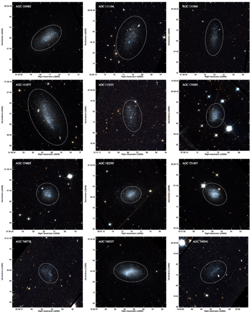
Figure 1.— HST 3-color images of the SHIELD galaxies; these images are reproductions of those in McQuinn et al. (2014). Overlaid on each panel is a single elliptical aperture to demonstrate the position and orientation of the elliptical apertures that were used in surface brightness analysis.

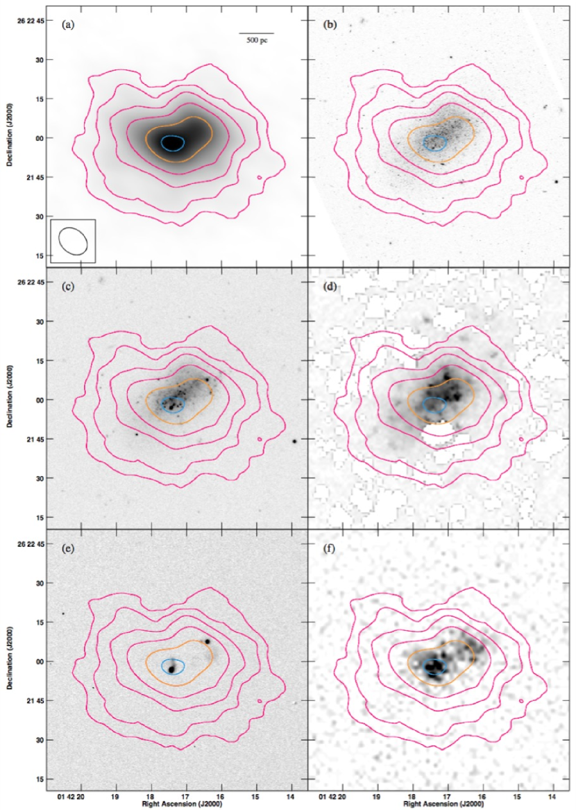
Figure 2.— AGC 110482 in VLA H I (a), HST F606W (b), KPNO WIYN 3.5m B-band (c), Spitzer 3.6 $\mu$m (d), KPNO WIYN 3.5m continuum-subtracted H$\alpha$ (e), and GALEX FUV (f). The H I column density contours, in units of 10²⁰ cm^-2, are overlaid at levels of (0.6125, 1.25, 2.5, 5, 10, 16). The highest two contour levels are highlighted in orange (10$\times$10²⁰ cm^-2) and blue (16$\times$10²⁰ cm^-2). The beam size of 11.98″$\times$9.04″ is shown in panel (a); the H I images are created using the robust-weighted, spectrally averaged data as discussed in Section 2.2.1.

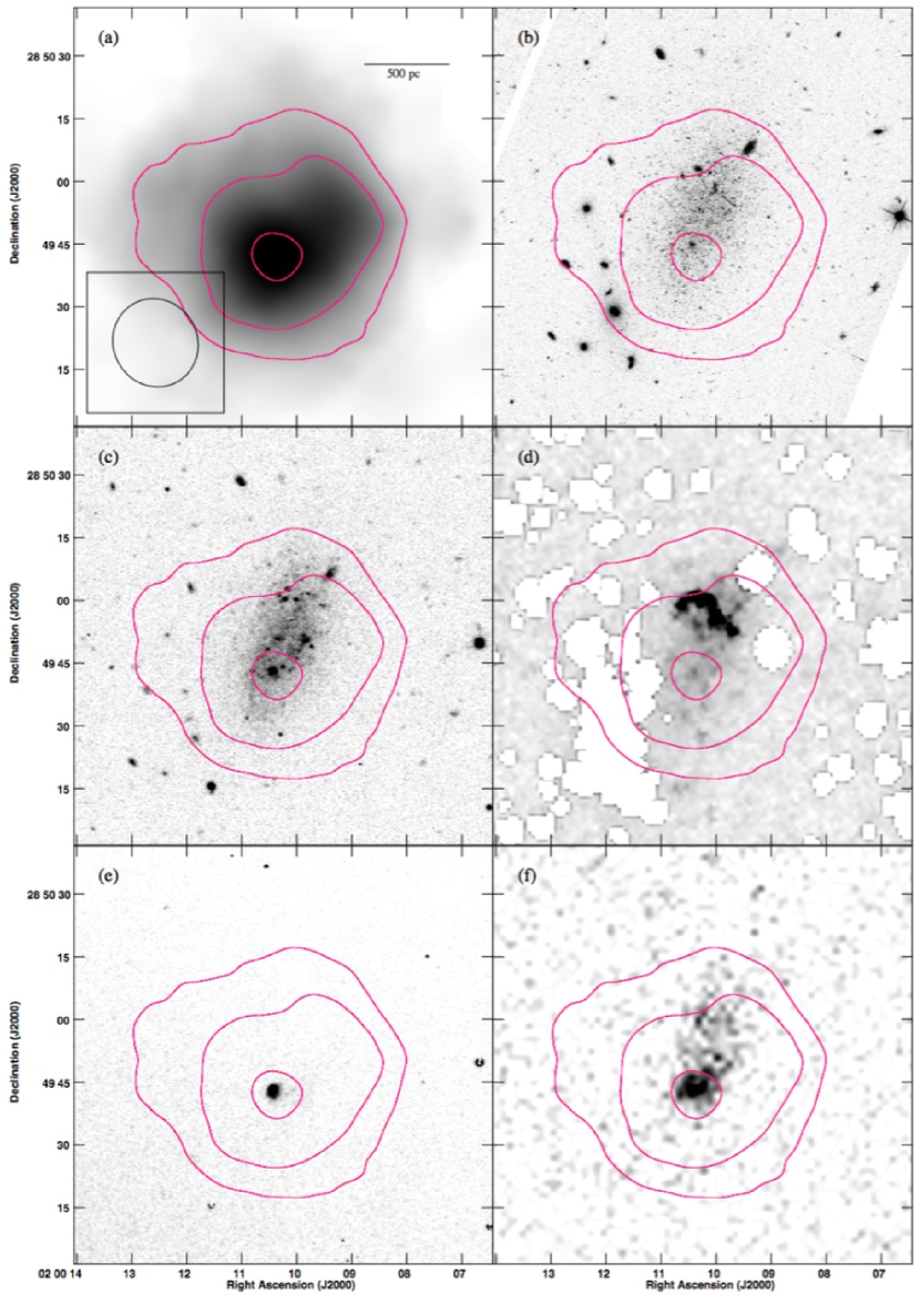
Figure 3.— AGC 111164 in VLA H I (a), HST F606W (b), KPNO WIYN 3.5m B-band (c), Spitzer 3.6 $\mu$m (d), KPNO WIYN 3.5m continuum-subtracted H$\alpha$ (e), and GALEX FUV (f). The H I column density contours, in units of 10²⁰ cm^-2, are overlaid at levels of (0.7, 1.4, 2.8). The beam size of 21.56″$\times$20.24″ is shown in panel (a); the H I images are created using the robust-weighted, spectrally averaged data as discussed in Section 2.2.1.

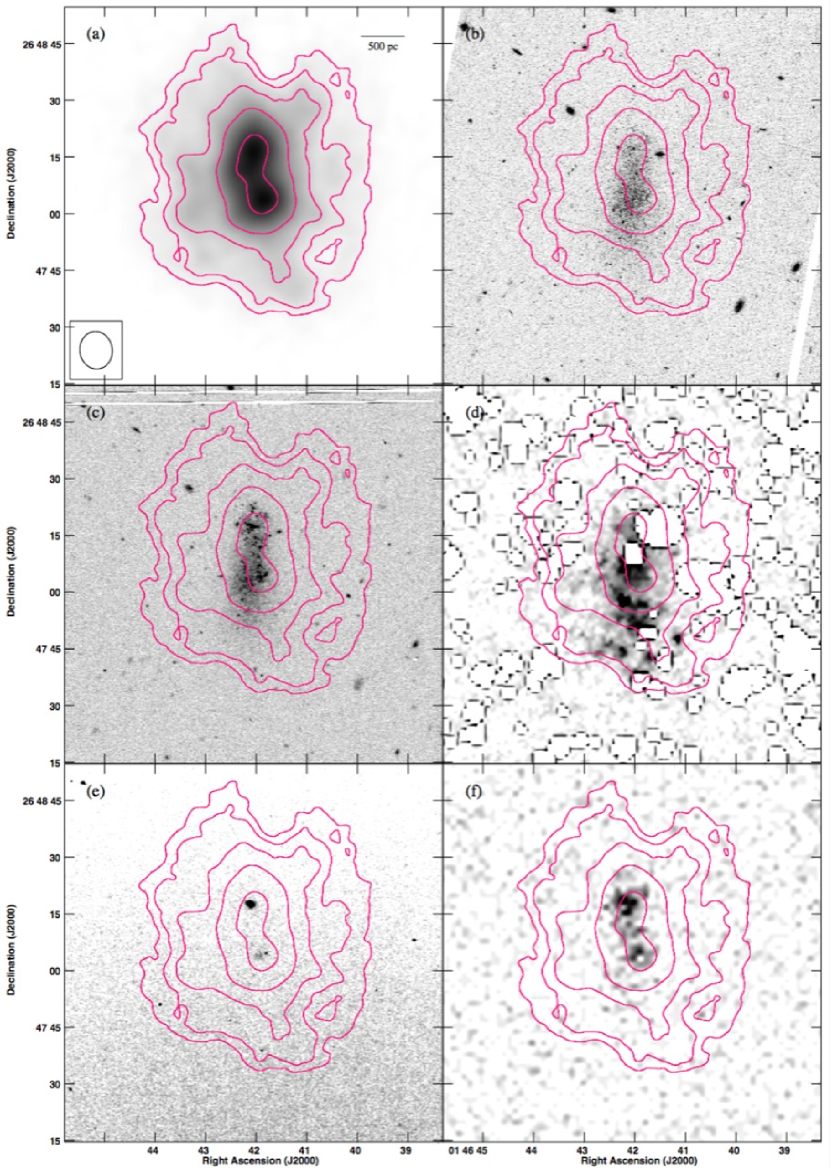
Figure 4.— AGC 111946 in VLA H I (a), HST F606W (b), KPNO WIYN 3.5m B-band (c), Spitzer 3.6 $\mu$m (d), KPNO WIYN 3.5m continuum-subtracted H$\alpha$ (e), and GALEX FUV (f). The H I column density contours, in units of 10²⁰ cm^-2, are overlaid at levels of (0.5, 1, 2, 4, 8). The beam size of 10.30″$\times$8.86″ is shown in panel (a); the H I images are created using the robust-weighted, spectrally averaged data as discussed in Section 2.2.1.

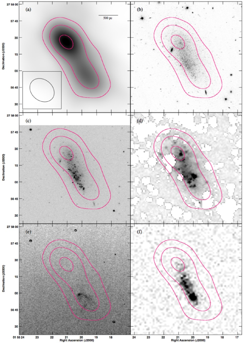
Figure 5.— AGC 111977 in VLA H I (a), HST F606W (b), KPNO WIYN 3.5m B-band (c), Spitzer 3.6 $\mu$m (d), KPNO WIYN 3.5m continuum-subtracted H$\alpha$ (e), and GALEX FUV (f). The H I column density contours, in units of 10²⁰ cm^-2, are overlaid at levels of (0.6125, 1.25, 2.5). The beam size of 24.01″$\times$19.95″ is shown in panel (a); the H I images are created using the robust-weighted, spectrally averaged data as discussed in Section 2.2.1.

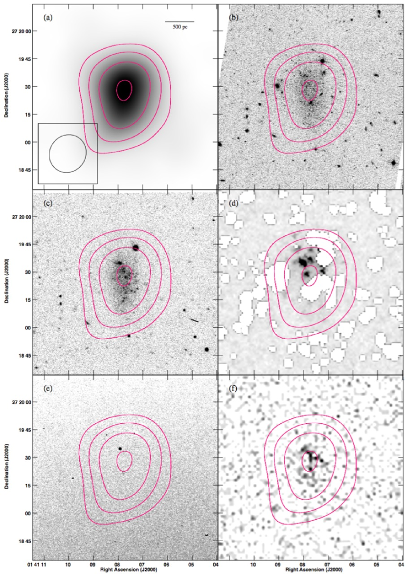
Figure 6.— AGC 112521 in VLA H I (a), HST F606W (b), KPNO WIYN 3.5m B-band (c), Spitzer 3.6 $\mu$m (d), KPNO WIYN 3.5m continuum-subtracted H$\alpha$ (e), and GALEX FUV (f). The H I column density contours, in units of 10²⁰ cm^-2, are overlaid at levels of (0.5625, 1.125, 2.25, 4.5). The beam size of 22.03″$\times$19.51″ is shown in panel (a); the H I images are created using the robust-weighted, spectrally averaged data as discussed in Section 2.2.1.

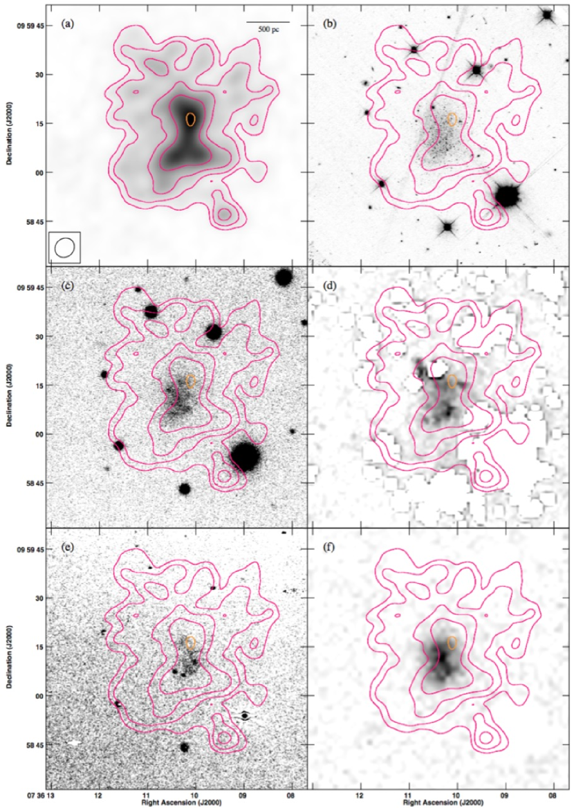
Figure 7.— AGC 174585 in VLA H I (a), HST F606W (b), KPNO WIYN 3.5m B-band (c), Spitzer 3.6 $\mu$m (d), KPNO WIYN 3.5m continuum-subtracted H$\alpha$ (e), and GALEX FUV (f). The H I column density contours, in units of 10²⁰ cm^-2, are overlaid at levels of (0.6125, 1.25, 2.5, 5, 10). The highest contour level is highlighted in orange (10$\times$10²⁰ cm^-2). The beam size of 6.19″$\times$5.52″ is shown in panel (a); the H I images are created using the robust-weighted, spectrally averaged data as discussed in Section 2.2.1.

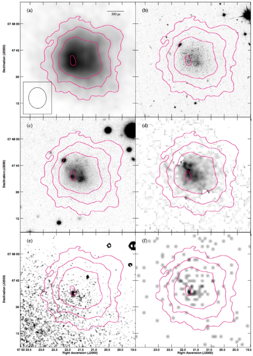
Figure 8.— AGC 174605 in VLA H I (a), HST F606W (b), KPNO WIYN 3.5m B-band (c), Spitzer 3.6 $\mu$m (d), KPNO WIYN 3.5m continuum-subtracted H$\alpha$ (e), and GALEX FUV (f). The H I column density contours, in units of 10²⁰ cm^-2, are overlaid at levels of (0.55, 1.1, 2.2, 4.4). The beam size of 11.81″$\times$9.99″ is shown in panel (a); the H I images are created using the robust-weighted, spectrally averaged data as discussed in Section 2.2.1.

Figure 9.— AGC 182595 in VLA H I (a), HST F606W (b), KPNO WIYN 3.5m B-band (c), Spitzer 3.6 $\mu$m (d), KPNO WIYN 3.5m continuum-subtracted H$\alpha$ (e), and GALEX FUV (f). The H I column density contours, in units of 10²⁰ cm^-2, are overlaid at levels of (0.75, 1.5, 3). The beam size of 10.05″$\times$9.93″ is shown in panel (a); the H I images are created using the robust-weighted, spectrally averaged data as discussed in Section 2.2.1.

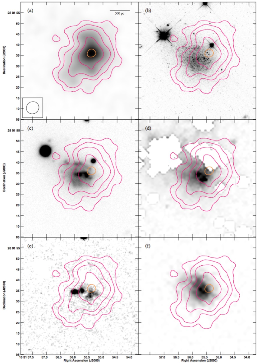
Figure 10.— AGC 731457 in VLA H I (a), HST F606W (b), KPNO WIYN 3.5m B-band (c), Spitzer 3.6 $\mu$m (d), KPNO WIYN 3.5m continuum-subtracted H$\alpha$ (e), and GALEX FUV (f). The H I column density contours, in units of 10²⁰ cm^-2, are overlaid at levels of (0.6125, 1.25, 2.5, 5, 10). The highest contour level is highlighted in orange (10$\times$10²⁰ cm^-2). The beam size of 6.04″$\times$5.53″ is shown in panel (a); the H I images are created using the robust-weighted, spectrally averaged data as discussed in Section 2.2.1.

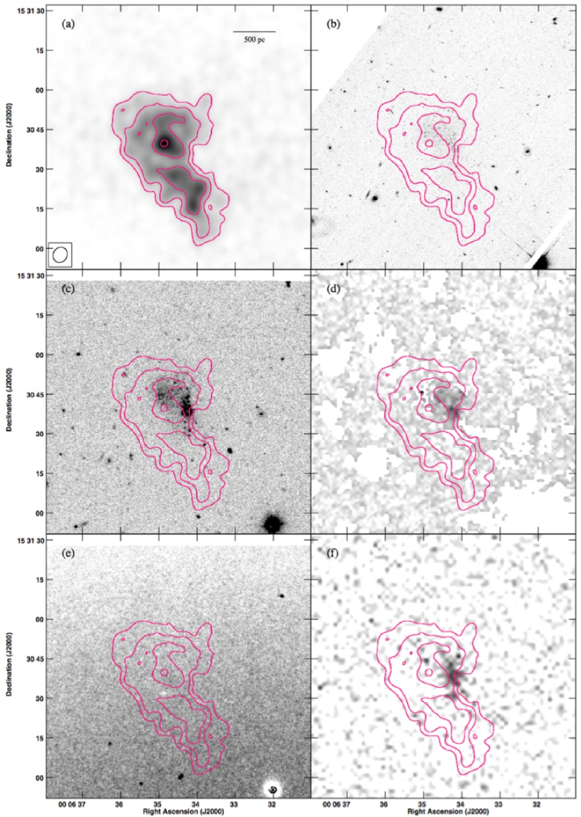
Figure 11.— AGC 748778 in VLA H I (a), HST F606W (b), KPNO WIYN 3.5m B-band (c), Spitzer 3.6 $\mu$m (d), KPNO WIYN 3.5m continuum-subtracted H$\alpha$ (e), and GALEX FUV (f). The H I column density contours, in units of 10²⁰ cm^-2, are overlaid at levels of (0.6875, 1.375, 2.75, 5.5). The beam size of 5.91″$\times$5.23″ is shown in panel (a); the H I images are created using the robust-weighted, spectrally averaged data as discussed in Section 2.2.1.

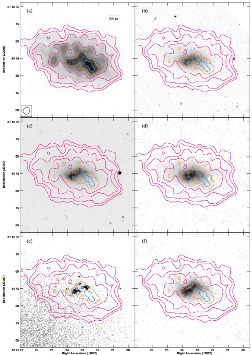
Figure 12.— AGC 749237 in VLA H I (a), HST F606W (b), KPNO WIYN 3.5m B-band (c), Spitzer 3.6 $\mu$m (d), KPNO WIYN 3.5m continuum-subtracted H$\alpha$ (e), and GALEX FUV (f). The H I column density contours, in units of 10²⁰ cm^-2, are overlaid at levels of (0.6125, 1.25, 2.5, 5, 10, 14). The highest two contour levels are highlighted in orange (10$\times$10²⁰ cm^-2) and blue (14$\times$10²⁰ cm^-2). The beam size of 6.21″$\times$5.59″ is shown in panel (a); the H I images are created using the robust-weighted, spectrally averaged data as discussed in Section 2.2.1.

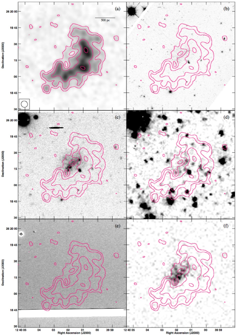
Figure 13.— AGC 749241 in VLA H I (a), HST F606W (b), KPNO WIYN 3.5m B-band (c), Spitzer 3.6 $\mu$m (d), KPNO WIYN 3.5m continuum-subtracted H$\alpha$ (e), and GALEX FUV (f). The H I column density contours, in units of 10²⁰ cm^-2, are overlaid at levels of (0.6125, 1.25, 2.5, 5). The beam size of 6.06″$\times$5.82″ is shown in panel (a); the H I images are created using the robust-weighted, spectrally averaged data as discussed in Section 2.2.1.

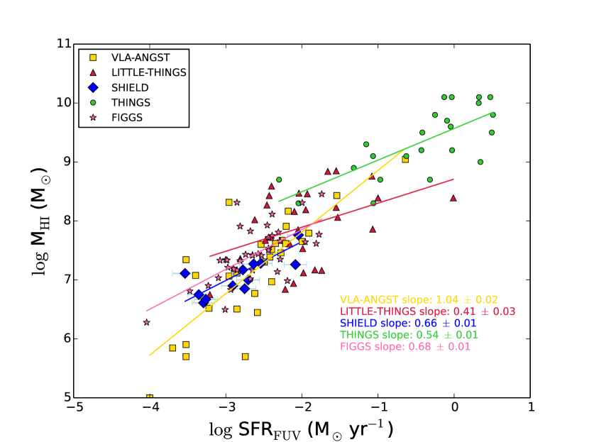
Figure 14.— M${}_{\rm H~{}{\sc I}}$ vs. SFR_FUV for the 12 SHIELD galaxies. Data from four other nearby galaxy surveys are included for comparison: VLA-ANGST (Ott et al., 2012), LITTLE-THINGS (Hunter et al., 2012), THINGS (Walter et al., 2008), and FIGGS (Roychowdhury et al., 2014). For each galaxy sample, we fit a linear regression for the slope and show these values at lower right. The most similar trends can be seen in the SHIELD and FIGGS datasets; this is not surprising, given that both surveys were selected to study low-mass, gas-rich systems. Note that while a significant portion of the sources from the low-mass surveys lie in the space where log(SFR_FUV) $\lesssim$ -2.5, very few of these sources have log(M${}_{\rm H~{}{\sc I}}$) $\gtrsim$ 7.5; galaxies which are forming fewer stars have smaller H I reservoirs.

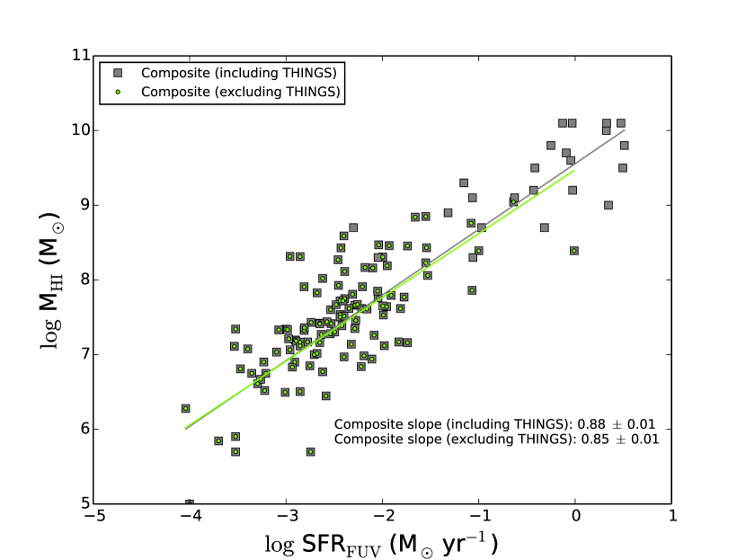
Figure 15.— M${}_{\rm H~{}{\sc I}}$ vs. SFR_FUV for all surveys shown in Figure 14. Two fits are shown: one to the composite sample of all galaxies (black line) and another to all galaxies excluding the THINGS sources. The slopes of the two lines are essentially indistinguishable.

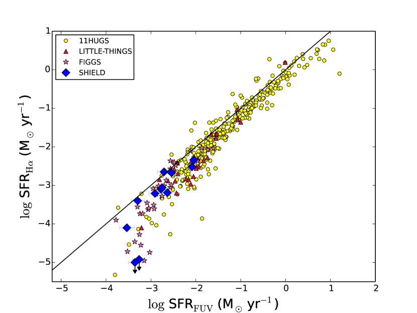
Figure 16.— SFR_Hα vs. SFR_FUV for the SHIELD sample. The line plotted shows equality. The bottom-most points for SHIELD represent the H$\alpha$ SFRs for AGC 748778 and AGC 749241, which are both formally upper limits.

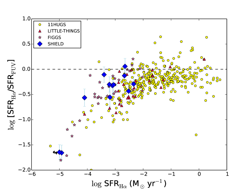
Figure 17.— SFR ratio [H$\alpha$/FUV] vs. SFR_Hα for the SHIELD sample. Data from three other nearby galaxy surveys are included for comparison: 11HUGS (Lee et al., 2009), LITTLE-THINGS (Hunter et al., 2012), and FIGGS (Roychowdhury et al., 2014).

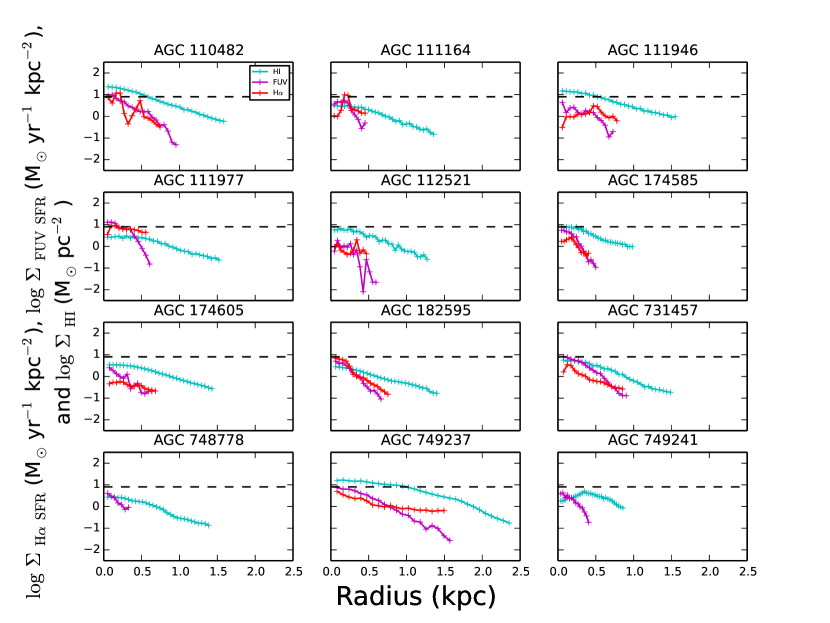
Figure 18.— $\Sigma_{\rm H~{}{\sc I}}$ (cyan), $\Sigma_{\rm H\alpha\ SFR}$ (red, from the Kennicutt 1998 prescription), and $\Sigma_{\rm FUV\ SFR}$ (magenta) vs. radius in kpc for each of the sample members. Only points measured at high confidence (greater than 3 $\sigma$) are shown. These radial profiles demonstrate the variety of distributions of star-forming regions and gas in the galaxies. FUV data for AGC 749237 is based on a conversion from the associated NUV counts. AGC 748778 and AGC 749241 are non-detections in H$\alpha$. The horizontal axis is set by the physically largest system, AGC 749237. The horizontal dashed line represents the HI column density threshold of 10²¹ cm^-2.

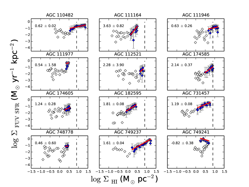
Figure 19.— $\Sigma_{\rm FUV\ SFR}$ vs. $\Sigma_{\rm H~{}{\sc I}}$ for each of the sample members. The slope of the line is the N index in the Kennicutt-Schmidt relation and is included in Table 6. The white points are below our 5$\sigma$ noise threshold and thus are not included in the calculation of the trendline of the data. The average value for the slope is N $\approx$ 1.50$\pm$0.02. The dashed vertical line represents an H I column density of 10²¹ atoms cm^-2.

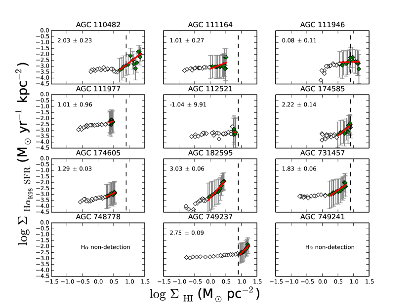
Figure 20.— $\Sigma_{\rm H\alpha\ SFR}$ vs. $\Sigma_{\rm H~{}{\sc I}}$ for each of the sample members, using the SFR_Hα derived from the Kennicutt (1998a) prescription. The slope of the line is the N index in the Kennicutt-Schmidt relation and is included in Table 6. The white points are below our 5$\sigma$ noise threshold and thus are not included in the calculation of the trendline of the data. The average value for the slope is N $\approx$ 0.34$\pm$0.02. The dashed vertical line represents an H I column density of 10²¹ atoms cm^-2.

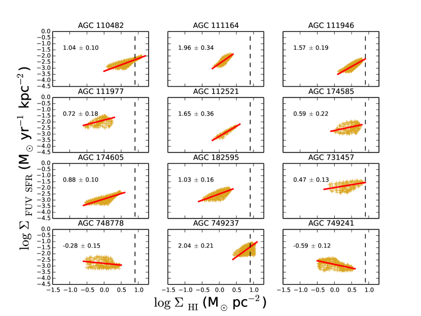
Figure 21.— $\Sigma_{\rm FUV\ SFR}$ vs. $\Sigma_{\rm H~{}{\sc I}}$ for each of the sample members. The points plotted are from the pixel-by-pixel correlation process described in Section 3. All FUV pixel values are above the 10% contour level for each source (i.e., all pixels plotted are greater than 10% of the peak flux), and the same is true of the H I values relative to the peak H I column density. The slope of the line is the N index in the Kennicutt-Schmidt relation and is included in Table 6. The average value for the slope is $N$ $\approx$ 0.68$\pm$0.04. A positive slope indicates high FUV and H I emission in the same pixels. The dashed vertical line represents the column density threshold of 1$\times$10²¹ atoms cm^-2.

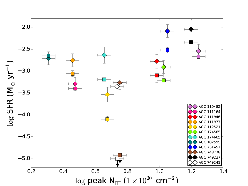
Figure 22.— UV and H$\alpha$-based SFR vs. peak H I column density for each of the sample members. FUV values are represented by diamonds and H$\alpha$ values are represented by squares. In some cases the error bars are smaller than the points themselves. The bottom-most two points represent upper-limits on the H$\alpha$ SFRs for AGC 748778 and AGC 749241 (formally non-detections).

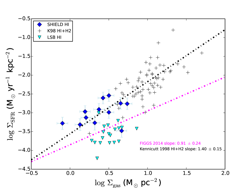
Figure 23.— $\Sigma_{\rm SFR_{\rm FUV}}$ vs. $\Sigma_{\rm H~{}{\sc I}}$ for the SHIELD sample. Data from a study of LSB galaxies (Wyder et al., 2009) and slopes from studies of normal spiral galaxies (Kennicutt, 1998b) and FIGGS dwarf irregular galaxies (Roychowdhury et al., 2014) are shown for comparison; note that different SFR metrics are used from one survey to the next. While the LSB galaxies lie below the canonical power-law slope, both studies of low-mass dwarfs appear to have shallower K-S relations than the higher-mass spiral galaxies. Note that the data from (Kennicutt, 1998b) is for HI+H2, while the other studies use just HI but assume the molecular contribution is negligible.

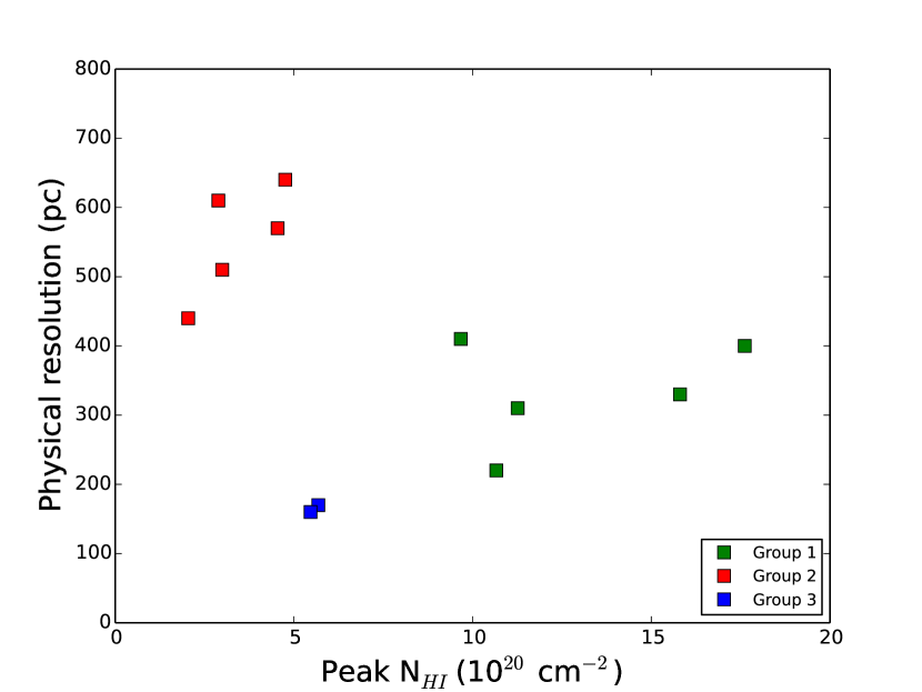
Figure 24.— Physical resolution in pc vs. peak H I column density for the SHIELD sample. The galaxies are grouped in the manner described in Section 4.2 according to their similar properties. While 2 of the 5 galaxies in Group 1 have the largest distances in the sample, the presence of B-configuration data results in smaller beam dimensions and fine resolution elements, allowing us to see the highest column density HI gas. In Group 2, 3 of the 5 galaxies lack B-configuration data, which contributes to their coarser resolution elements and inability to detect higher column density HI gas. The Group 3 galaxies are the outliers: the inclusion of B-configuration data provides fine resolution elements, but the galaxies are low-mass and devoid of higher column density HI gas.

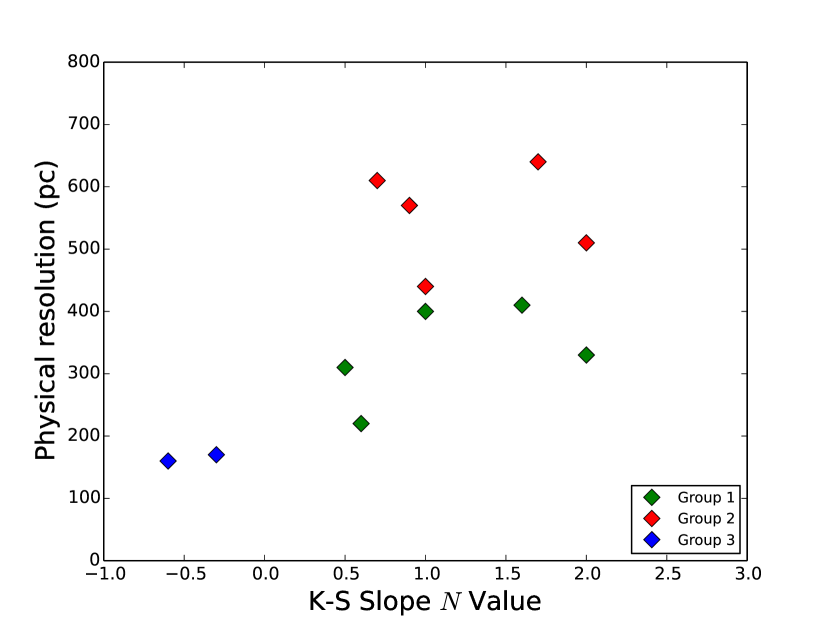
Figure 25.— Physical resolution in pc vs. $N$ value (the derived slope for the Kennicutt-Schmidt relation) for the SHIELD sample. The galaxies are grouped in the manner described in Section 4.2 according to their similar properties. While the members of Groups 1 and 2 can be characterized by differing physical resolution elements, they both have similar range and dispersion in terms of their $N$ values. Group 3 is the obvious outlier, hosting the only two galaxies with negative $N$ values. It is apparent that on sufficiently small scales, the K-S relation is no longer valid.

References

- Begum et al. (2008) Begum, A., Chengalur, J. N., Karachentsev, I. D., Sharina, M. E., & Kaisin, S. S. 2008, MNRAS, 386, 1667
- Bell & Kennicutt (2001) Bell, E. F., & Kennicutt, R. C., Jr. 2001, ApJ, 548, 681
- Bigiel et al. (2010) Bigiel, F., Leroy, A., Walter, F., et al. 2010, AJ, 140, 1194
- Bigiel et al. (2008) Bigiel, F., Leroy, A., Walter, F., et al. 2008, AJ, 136, 2846
- Bolatto et al. (2013) Bolatto, A. D., Wolfire, M., & Leroy, A. K. 2013, ARA&A, 51, 207
- Boselli et al. (2009) Boselli, A., Boissier, S., Cortese, L., et al. 2009, ApJ, 706, 1527
- Buat et al. (2005) Buat, V., Iglesias-Páramo, J., Seibert, M., et al. 2005, ApJ, 619, L51
- Burgarella et al. (2005) Burgarella, D., Buat, V., & Iglesias-Páramo, J. 2005, MNRAS, 360, 1413
- Cannon et al. (2011) Cannon, J. M., Giovanelli, R., Haynes, M. P., et al. 2011, ApJ, 739, LL22
- da Silva et al. (2014) da Silva, R. L., Fumagalli, M., & Krumholz, M. R. 2014, MNRAS, 444, 3275
- Elmegreen (2011) Elmegreen, B. G. 2011, EAS Publications Series, 51, 3
- Fazio et al. (2004) Fazio, G. G., Hora, J. L., Allen, L. E., et al. 2004, ApJS, 154, 10
- Filho et al. (2016) Filho, M. E., Sánchez Almeida, J., Amorín, R., et al. 2016, ApJ, 820, 109
- Fisher & Tully (1975) Fisher, J. R., & Tully, R. B. 1975, A&A, 44, 151
- Giovanelli et al. (2005) Giovanelli, R., Haynes, M. P., Kent, B. R., et al. 2005, AJ, 130, 2598
- Giovanelli & Haynes (1988) Giovanelli, R., & Haynes, M. P. 1988, Galactic and Extragalactic Radio Astronomy, 522
- Hagen et al. (2014) Hagen, C., Cannon, J. M., Cave, I., et al. 2014, American Astronomical Society Meeting Abstracts #223, 223, #355.16
- Hao et al. (2011) Hao, C.-N., Kennicutt, R. C., Johnson, B. D., et al. 2011, ApJ, 741, 124
- Haurberg (2013) Haurberg, N. C. 2013, Ph.D. Thesis,
- Haurberg et al. (2015) Haurberg, N. C., Salzer, J. J., Cannon, J. M., & Marshall, M. V. 2015, ApJ, 800, 121
- Haynes et al. (2011) Haynes, M. P., Giovanelli, R., Martin, A. M., et al. 2011, AJ, 142, 170
- Huang et al. (2012) Huang, S., Haynes, M. P., Giovanelli, R., & Brinchmann, J. 2012, ApJ, 756, 113
- Hunter et al. (2012) Hunter, D. A., Ficut-Vicas, D., Ashley, T., et al. 2012, AJ, 144, 134
- Jörsäter & van Moorsel (1995) Jörsäter, S., & van Moorsel, G. A. 1995, AJ, 110, 2037
- Kennicutt (1983) Kennicutt, R. C., Jr. 1983, ApJ, 272, 54
- Kennicutt (1998a) Kennicutt, R. C., Jr. 1998, ARA&A, 36, 189
- Kennicutt (1998b) Kennicutt, R. C., Jr. 1998, ApJ, 498, 541
- Kennicutt & Evans (2012) Kennicutt, R. C., & Evans, N. J. 2012, ARA&A, 50, 531
- Kirby et al. (2012) Kirby, E. M., Koribalski, B., Jerjen, H., & López-Sánchez, Á. 2012, MNRAS, 420, 2924
- Krumholz (2013) Krumholz, M. R. 2013, MNRAS, 436, 2747
- Krumholz (2012) Krumholz, M. R. 2012, ApJ, 759, 9
- Lee et al. (2009) Lee, J. C., Gil de Paz, A., Tremonti, C., et al. 2009, ApJ, 706, 599
- Lee et al. (2016) Lee, J. C., Veilleux, S., McDonald, M., Hilbert, B. 2016, ApJ, 817, 177
- Leroy et al. (2008) Leroy, A. K., Walter, F., Brinks, E., et al. 2008, AJ, 136, 2782
- Marshall (2013) Marshall, M. 2013, American Astronomical Society Meeting Abstracts #221, 221, #352.05
- Martin et al. (2005) Martin, D. C., Fanson, J., Schiminovich, D., et al. 2005, ApJ, 619, L1
- Martin et al. (2010) Martin, A. M., Papastergis, E., Giovanelli, R., et al. 2010, ApJ, 723, 1359
- Masters (2005) Masters, K. L. 2005, Ph.D. Thesis, Cornell University
- McNichols et al. (2016) McNichols, A. T., Teich, Y. G., Nims, E., Cannon, J. M., et al. 2016, ApJ, submitted
- McMullin et al. (2007) McMullin, J. P., Waters, B., Schiebel, D., Young, W., & Golap, K. 2007, Astronomical Data Analysis Software and Systems XVI, 376, 127
- McQuinn et al. (2015a) McQuinn, K. B. W., Cannon, J. M., Dolphin, A. E., et al. 2015, ApJ, 802, 66
- McQuinn et al. (2015b) McQuinn, K. B. W., Skillman, E. D., Dolphin, A. E., & Mitchell, N. P. 2015, ApJ, 808, 109
- McQuinn et al. (2014) McQuinn, K. B. W., Cannon, J. M., Dolphin, A. E., et al. 2014, ApJ, 785, 3
- Meurer et al. (2009) Meurer, G. R., Wong, O. I., Kim, J. H., et al. 2009, ApJ, 695, 765
- Michalowski et al. (2015) Michałowski, M. J., Gentile, G., Hjorth, J., et al. 2015, A&A, 582, A78
- Momose et al. (2013) Momose, R., Koda, J., Kennicutt, R. C., Jr., et al. 2013, ApJ, 772, L13
- Morrissey et al. (2007) Morrissey, P., Conrow, T., Barlow, T. A., et al. 2007, ApJS, 173, 682
- Ott et al. (2012) Ott, J., Stilp, A. M., Warren, S. R., et al. 2012, AJ, 144, 123
- Roychowdhury et al. (2009) Roychowdhury, S., Chengalur, J. N., Begum, A., & Karachentsev, I. D. 2009, The Low-Frequency Radio Universe, 407, 106
- Roychowdhury et al. (2011) Roychowdhury, S., Chengalur, J. N., Kaisin, S. S., Begum, A., & Karachentsev, I. D. 2011, MNRAS, 414, L55
- Roychowdhury et al. (2014) Roychowdhury, S., Chengalur, J. N., Kaisin, S. S., & Karachentsev, I. D. 2014, MNRAS, 445, 1392
- Roychowdhury et al. (2015) Roychowdhury, S., Huang, M.-L., Kauffmann, G., Wang, J., & Chengalur, J. N. 2015, MNRAS, 449, 3700
- Salim et al. (2007) Salim, S., Rich, R. M., Charlot, S., et al. 2007, ApJS, 173, 267
- Schmidt (1959) Schmidt, M. 1959, ApJ, 129, 243
- Schlafly & Finkbeiner (2011) Schlafly, E. F., & Finkbeiner, D. P. 2011, ApJ, 737, 103
- Schlegel et al. (1998) Schlegel, D. J., Finkbeiner, D. P., & Davis, M. 1998, ApJ, 500, 525
- Schruba et al. (2012) Schruba, A., Leroy, A. K., Walter, F., et al. 2012, AJ, 143, 138
- Schruba et al. (2010) Schruba, A., Leroy, A. K., Walter, F., Sandstrom, K., & Rosolowsky, E. 2010, ApJ, 722, 1699
- Skillman (1987) Skillman, E. D. 1987, NASA Conference Publication, 2466, 263
- Swaters et al. (2002) Swaters, R. A., van Albada, T. S., van der Hulst, J. M., & Sancisi, R. 2002, A&A, 390, 829
- Taylor et al. (1998) Taylor, C. L., Kobulnicky, H. A., & Skillman, E. D. 1998, Magellanic Clouds and Other Dwarf Galaxies, 205
- Walter et al. (2008) Walter, F., Brinks, E., de Blok, W. J. G., et al. 2008, AJ, 136, 2563-2647
- Warren et al. (2015) Warren, S. R., Molter, E., Cannon, J. M., et al. 2015, ApJ, 814, 30
- Werner et al. (2004) Werner, M. W., Roellig, T. L., Low, F. J., et al. 2004, ApJS, 154, 1
- Wyder et al. (2007) Wyder, T. K., Martin, D. C., Schiminovich, D., et al. 2007, ApJS, 173, 293
- Wyder et al. (2009) Wyder, T. K., Martin, D. C., Barlow, T. A., et al. 2009, ApJ, 696, 1834
- Fumagalli et al. (2011) Fumagalli, M., da Silva, R. L., & Krumholz, M. R. 2011, ApJ, 741, L26
- da Silva et al. (2012) da Silva, R. L., Fumagalli, M., & Krumholz, M. 2012, ApJ, 745, 145
- Eldridge (2012) Eldridge, J. J. 2012, MNRAS, 422, 794
- Weisz et al. (2012) Weisz, D. R., Johnson, B. D., Johnson, L. C., et al. 2012, ApJ, 744, 44