Identifying galaxy candidates in WSRT H i imaging of ultra-compact high velocity clouds

Ultra-compact high velocity clouds (UCHVCs) were identified in the Arecibo Legacy Fast ALFA (ALFALFA) H i survey as potential gas-bearing dark matter halos. Here we present higher resolution neutral hydrogen (H i) observations of twelve UCHVCS with the Westerbork Synthesis Radio Telescope (WSRT). The UCHVCs were selected based on a combination of size, isolation, large recessional velocity and high column density as the best candidate dark matter halos. The WSRT data were tapered to image the UCHVCs at 210^′′ (comparable to the Arecibo resolution) and 105^′′ angular resolution. In a comparison of the single-dish to interferometer data, we find that the integrated line flux recovered in the WSRT observations is generally comparable to that from the single-dish ALFALFA data. In addition, any structure seen in the ALFALFA data is reproduced in the WSRT maps at the same angular resolution. At 210^′′ resolution all the sources are generally compact with a smooth H i morphology, as expected from their identification as UCHVCs. At the higher angular resolution, a majority of the sources break into small clumps contained in a diffuse envelope. These UCHVCs also have no ordered velocity motion and are most likely Galactic halo clouds. We identify two UCHVCs, AGC 198606 and AGC 249525, as excellent galaxy candidates based on maintaining a smooth H i morphology at higher angular resolution and showing ordered velocity motion consistent with rotation. A third source, AGC 249565, lies between these two populations in properties and is a possible galaxy candidate. If interpreted as gas-bearing dark matter halos, the three candidate galaxies have rotation velocities of $8-15$ km s^-1, H i masses of $0.6-50\times 10^{5}$ $M_{\odot}$, H i radii of $0.3-2$ kpc, and dynamical masses of $2-20\times 10^{7}$ $M_{\odot}$ for a range of plausible distances. These are the UCHVCs with the highest column density values in the ALFALFA H i data and we suggest this is the best way to identify further candidates.

1 Introduction

Studying the properties of the smallest galaxies is important both for testing $\Lambda$CDM and understanding galaxy formation. $\Lambda$CDM does an excellent job of describing large scale structure and the distribution of massive galaxies (e.g., Vogelsberger et al. 2014). However, on small scales, there are tensions between observations of dwarf galaxies and predictions from simulations for both field dwarf galaxies and satellite dwarf galaxies in the Milky Way (MW). These tensions include the total number count of expected galaxies (e.g., the ”missing satellites problem” in the Local Group; Kauffmann et al. 1993; Klypin et al. 1999; Moore et al. 1999; Martin et al. 2010; Papastergis et al. 2011); which dark matter halos host galaxies (e.g., the ”too big too fail” problem; Boylan-Kolchin et al. 2012; Papastergis et al. 2015); and the structure of those dark matter halos (e.g., the ”cusp-core” problem; de Blok et al. 2008; Walker & Peñarrubia 2011). Much work exists to suggest that these differences can be reconciled by the proper inclusion of baryonic physics in simulations (e.g., Oh et al. 2011; Oñorbe et al. 2015; Sawala et al. 2016; Wetzel et al. 2016). However, much of the relevant physics is implemented at the sub-grid level, and simulations of dwarf galaxies are sensitive to (at least some of) these parameters (e.g., Busha et al. 2010; Simpson et al. 2013; Vandenbroucke et al. 2016), and results between various simulations do not necessarily agree (e.g., the existence of a $M_{*}$-$M_{halo}$ relation at low masses, Sawala et al. 2015; Oñorbe et al. 2015; Wheeler et al. 2015). Part of the issue may be resolution; as the resolution of simulations increases, typically the lowest mass galaxy that can form in the simulation also decreases (Hoeft et al. 2006; Wheeler et al. 2015).

The existence of extremely low-mass galaxies that have a significant reservoir of neutral hydrogen (H i) also challenges our understanding of how the smallest galaxies form and evolve. How have these galaxies maintained their gas reservoir given the multitude of baryonic processes that can disrupt it? The most extreme example is Leo T; this galaxy has an H i mass of only $2.8\times 10^{5}$ $M_{\odot}$ and a stellar mass of $1.05\times 10^{5}$ $M_{\odot}$ (Ryan-Weber et al. 2008; Weisz et al. 2012). The recent discovery of Leo P demonstrates that there are more low-mass gas-dominated systems to be discovered. Leo P has an H i mass of $8.1\times 10^{5}$ and a stellar mass of $5.6\times 10^{5}$ $M_{\odot}$ (McQuinn et al. 2015). Both systems are very faint optically; Leo T is on the edge of detection for the Sloan Digital Sky Survey (SDSS, Kravtsov 2010), and Leo P was originally identified as an H i source (Giovanelli et al. 2013). This highlights a parameter space for H i surveys for understanding the smallest galaxies. Galaxies similar to Leo T or Leo P but that lie at larger distances or have had slightly different star formation histories (e.g., less recent star formation) might be missed by optical surveys but detected in blind H i surveys.

To this end, Giovanelli et al. (2010) presented the idea that ultra-compact high velocity clouds (UCHVCs) in the Arecibo Legacy Fast ALFA (ALFALFA) H i survey may be gas in dark matter halos with a stellar counterpart not detectable in extant optical surveys. Adams et al. (2013, hereafter A13) built on this work, presenting a catalog of sources with specific selection criteria for the 40% complete ALFALFA survey. Similarly, Saul et al. (2012) presented a catalog of compact H i clouds from GALFA H i survey, highlighting those that were potentially good galaxy candidates. These catalogs represent an excellent starting point for identifying potential gas-bearing dark matter halos in the local universe, and theoretical models suggest they contain good candidates (e.g., Faerman et al. 2013). However, without stellar counterparts there are no direct distances to these clouds and they may be local clouds of gas that arise from various Galactic processes. Determining which single-dish H i properties of these clouds are the best predictor that a system is a good candidate to be gas in a dark matter halo, rather than a local H i cloud, is critical for making the most use of expensive follow-up observations.

The most straightforward approach for understanding the nature of the UCHVCs would be to detect an optical counterpart, constraining the distance to the system and identifying it as a bona-fide galaxy. Previous work has shown that stellar counterparts for UCHVCs appear to be rare and correspond to more distant, massive systems with typical H i masses of $\sim 10^{7}$ $M_{\odot}$ (Bellazzini et al. 2015; Sand et al. 2015). However, Janesh et al. (2015) identified a tentative optical counterpart for one UCHVC, AGC 198606, at a distance of 383 kpc. This distance is consistent with the hypothesis that this UCHVC is a companion to Leo T, located only 1.2^∘ and 17 km s^-1 away. At this distance, AGC  198606 has an H i mass of $5\times 10^{5}$ $M_{\odot}$, comparable to that of Leo T, while its stellar mass is an order of magnitude lower.

The lack of definitive stellar counterparts to date may indicate that UCHVCs representing gas-bearing dark matter halos are rare. Alternatively, it could also be a result of these systems having intrinsically faint stellar counterparts; in the case above, AGC 198606 has $M_{\mathrm{HI}}$/$M_{*}$$>40$. The ability to better distinguish the best candidates could help address which of these scenarios is dominant. Previous work with high velocity clouds (HVCs), and especially compact HVCs (previously proposed as ”dark” galaxies), has shown that higher resolution H i imaging can be used to constrain the nature of these systems and to address whether they are Galactic or extragalactic (e.g., de Heij et al. 2002; Brüns & Westmeier 2004; Westmeier et al. 2005a; Faridani et al. 2014).

Hence we present resolved H i observations with the Westerbork Synthesis Radio Telescope (WSRT) data for twelve UCHVCs in order to help address their nature. The sources are drawn from a catalog of UCHVCs following the selection criteria of A13 but including expanded sky coverage of the ALFALFA H i survey. Importantly, the restriction that $|v_{LSR}|>120$ km s^-1 was relaxed so that clouds close to Galactic H i velocities that were otherwise good candidates are included. The sources were selected to represent the best potential galaxy candidates on the basis of various properties: high average column density, as those systems with the highest density of gas and potential for star formation; small angular size, for the systems most consistent with being distant objects; isolation, as the objects least likely to be part of a larger Galactic HVC complex; and large recessional velocity, as it is difficult to explain in a Galactic fountain model. Every cloud was selected for at least one of these criterion; a few fulfilled multiple criteria. The goal is to determine which, if any, of these criteria are most important for identifying the best candidate galaxies.

In Section 2 we present the ALFALFA H i properties and the WSRT H i data for the twelve UCHVCs observed. In Section 3, we compare the ALFALFA and WSRT H i properties. In Section 4 we discuss the nature of the UCHVCs, how to identify the best galaxy candidates, and the properties of the galaxy candidates. We summarize our results in Section 5. The Appendix contains a full presentation of the data products for all the UCHVCs.

Table 1: ALFALFA H i properties

HVC name	AGC	R.A.+Dec.	cz	$W_{50}$	$\bar{a}$	$S_{HI}$	$M_{HI}$	$\log\bar{N}_{HI}$
		J2000	km s-1	km s-1	′	Jy km s-1	$M_{\odot}$	atoms cm-2
(1)	(2)	(3)	(4)	(5)	(6)	(7)	(8)	(9)
HVC214.76+42.45+44	198606	093005.4+163956	51	26 (1)	12.2	17.44 (0.05)	6.61	19.71
HVC204.88+44.86+147	198511	093013.2+241217	152	15 (1)	7.0	0.73 (0.03)	5.24	18.81
HVC205.83+45.14+173	198683	093208.0+233752	178	19 (1)	10.4	0.88 (0.04)	5.32	18.56
HVC217.77+58.67+96	208747	103706.6+203058	98	23 (1)	10.9	2.74 (0.05)	5.81	19.0
HVC212.68+62.39+64	208753	104932.4+235638	65	23 (1)	12.7	3.95 (0.07)	5.97	19.03
HVC230.27+71.10+76	219663	113429.7+201249	74	17 (1)	7.2	0.75 (0.03)	5.25	18.8
HVC235.38+74.79+195	219656	115124.3+203220	192	21 (1)	7.5	0.88 (0.04)	5.32	18.84
HVC271.57+79.03+248	229326	122734.7+173823	242	23 (8)	7.8	0.77 (0.04)	5.26	18.74
HVC276.53+79.84+255	229327	123231.6+175721	249	19 (1)	11.1	0.9 (0.05)	5.33	18.51
HVC028.09+71.87-142	249393	141054.9+241210	-155	38 (2)	12.7	1.02 (0.07)	5.38	18.44
HVC011.76+67.89+60	249525	141750.1+173252	48	24 (7)	8.5	6.36 (0.04)	6.18	19.59
HVC015.96+63.90+44	249565	143557.6+171004	30	18 (1)	7.5	1.76 (0.04)	5.62	19.14

2 Data

2.1 ALFALFA

ALFALFA is an extragalactic spectral line survey with the ALFA receiver at the Arecibo 305m telescope. The survey maps 7000 square degrees of sky over the spectral range 1335 to 1435 MHz (roughly -2500 km s^-1 to 17500 km s^-1 for the H i line), with a spectral resolution of 25 kHz, or $\sim 5.5$ km s^-1 at $z=0$ (Giovanelli et al. 2005, 2007). The UCHVCs are identified and measured independently of the standard ALFALFA pipeline, in order to properly account for their extended and low surface brightness nature compared to the standard ALFALFA sources. A full reporting of this methodology is given in A13. Here, we briefly summarize the key measured H i properties from the ALFALFA H i data. After automated identification, each source is visually inspected and remeasured. Relevant measured properties are the H i centroid, the major and minor axes of the half-flux ellipse, integrated line flux, velocity and linewidth. The geometric mean of the half-flux ellipse is used as a representative source size. In addition, for the UCHVCs, a representative column density value, $\bar{N}_{HI}$, is calculated following:

$$\bar{N}_{HI}[\mathrm{atoms\ cm}^{-2}]=4.4\times 10^{20}\leavevmode\nobreak\ \bar{a}^{-2}\leavevmode\nobreak\ S_{21}\,\,\,\,{\rm cm}^{-2},\\$$ (1)

where $\bar{a}$ is representative source size in arcminutes and $S_{21}$ the integrated H i flux density in Jy km s^-1. The final UCHVC catalog of A13 is constructed by including all sources with $|v_{LSR}|>120$ km s^-1, an H i major axis less than 30^′, a signal-to-noise (S/N) greater than eight, and that meet the isolation criteria. The isolation criteria are one of the most critical parameters for defining the UCHVC sample and full details are given in A13. The distance of a UCHVC from another source is parameterized as $D=\sqrt{\theta^{2}+(f\delta v)^{2}}$, where $\theta$ is the angular separation in degrees, $\delta v$ is the velocity separation in km s^-1, and $f$ is a factor that links a velocity separation to an angular separation. Sources must meet isolation three criteria: (1) visual inspection shows no connection to other H i structure; (2) the UCHVCs are separated from the classic HVCs of Wakker & van Woerden (1991, B. Wakker 2012, private communication) by $D>15$^∘ for $f=$ 0.5 ^∘/km s^-1; (3) and the UCHVCs have no more than 3 neighbors in the ALFALFA data within $D=3$^∘ for $f=0.2$^∘/km s^-1. In addition, a most-isolated subsample is defined where there are no more than 3 neighbors in the ALFALFA data within $D=10$^∘, a $\sim$30$\times$ larger region.

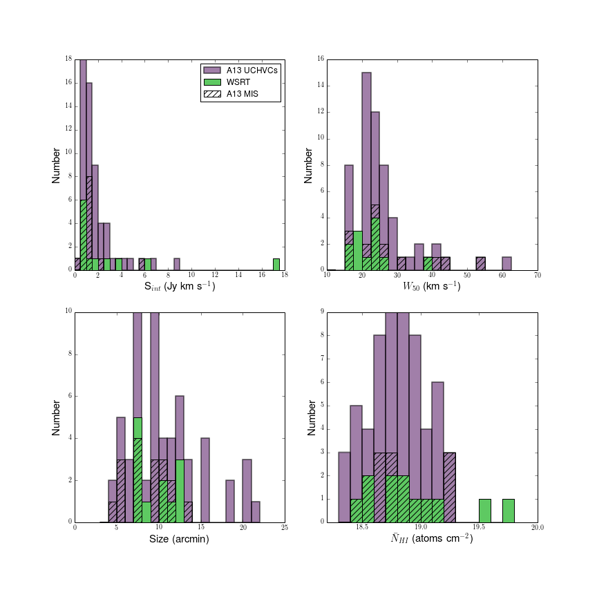
Figure 1: ALFALFA H i properties of the UCHVCs presented in this work compared to the ALFALFA H i properties of the catalog of A13, including the most-isolated subsample (MIS).

Two of the UCHVCs, AGC 198511 and AGC 249393, are included in the A13 catalog. A third UCHVC, AGC 198606, is presented independently in Adams et al. (2015) as an excellent galaxy candidate. These three UCHVCs, along with AGC 208747, AGC 219656, AGC 229326, AGC 229327 and AGC 249525, are included in the 70% ALFALFA catalog (Jones et al. 2016). The other four UCHVCs of this work have not been previously published. The ALFALFA H i properties of all of the UCHVCs of this work are reported in Table 1.

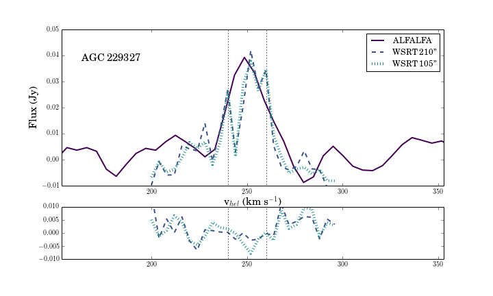
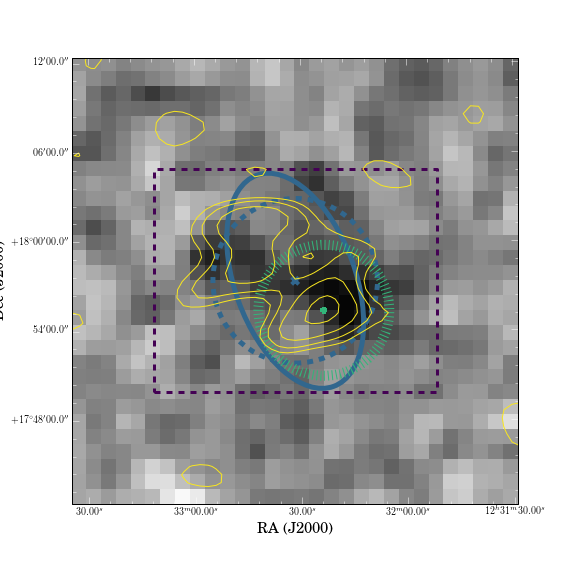
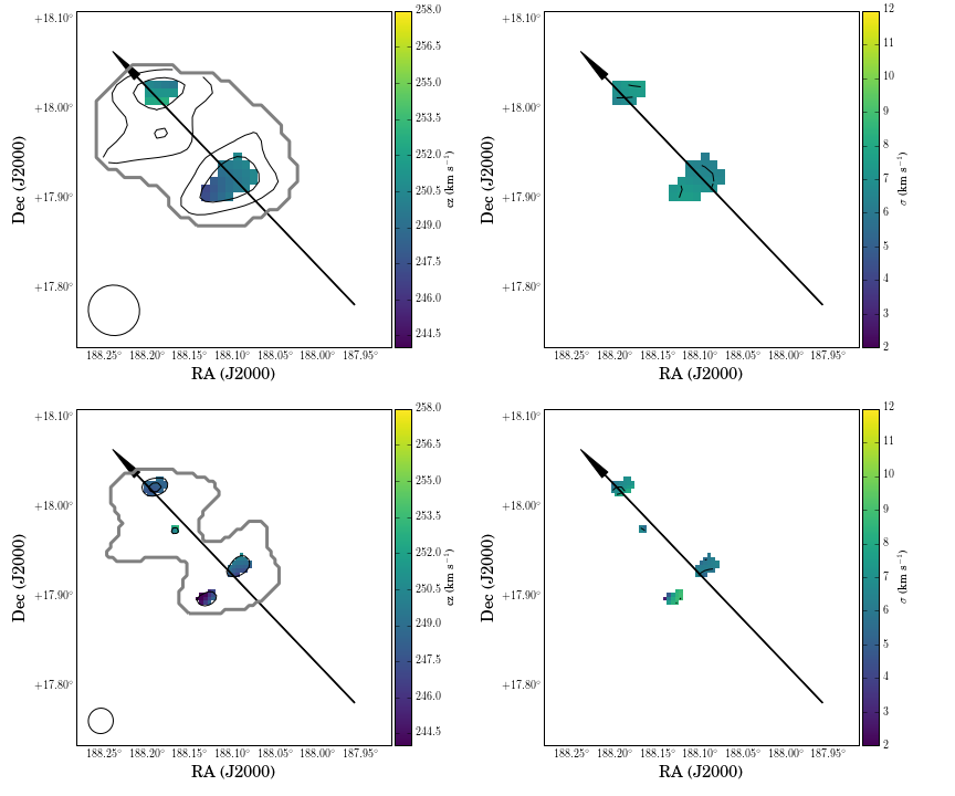
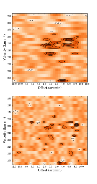
Figure 16: ALFALFA and WSRT data for AGC 229327 as in Figure 8 but with H i column density contours at [2, 3] $\times 10^{18}$ and [6, 8] $\times 10^{18}$ atoms cm^-2 for the 210^′′ and 105^′′ data and velocity contours at [248, 250, 252] km s^-1.

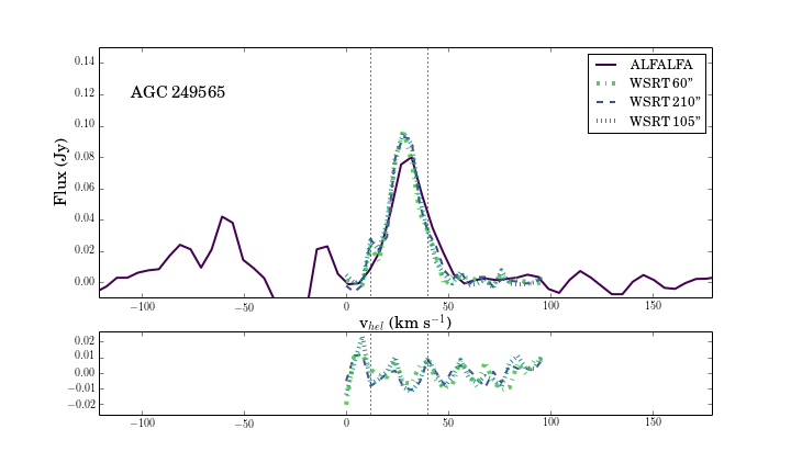
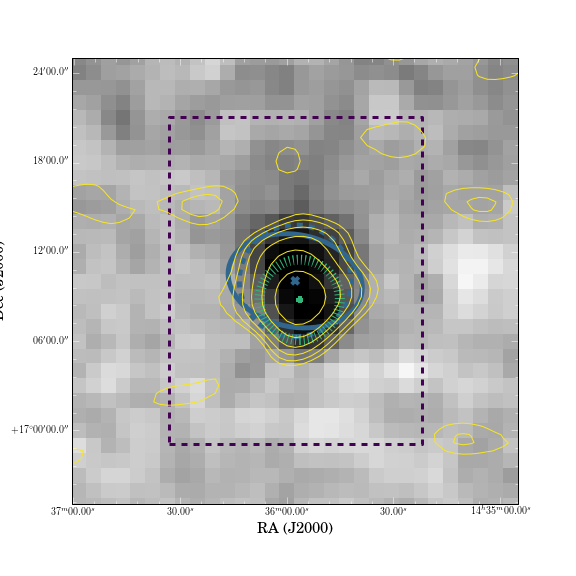
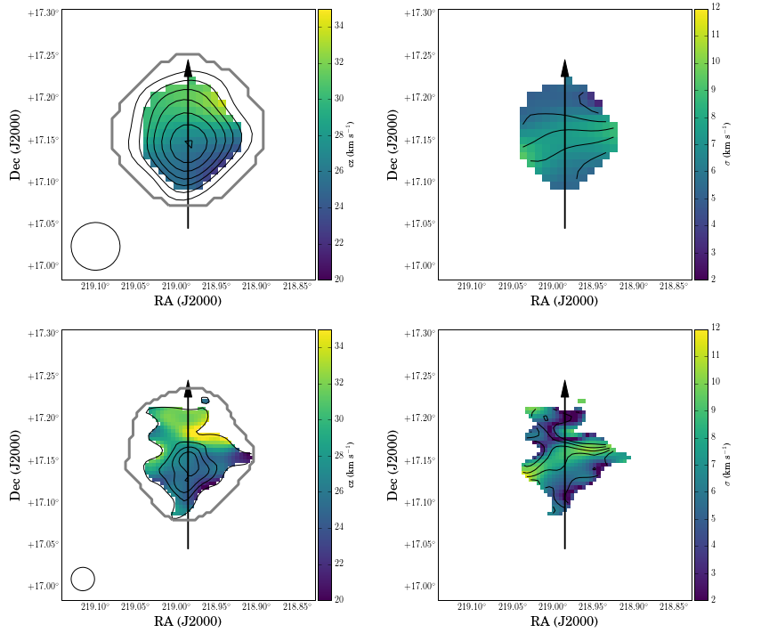
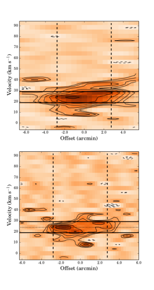
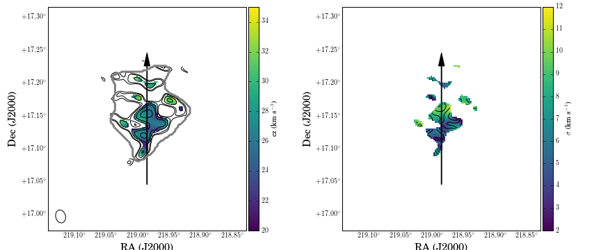
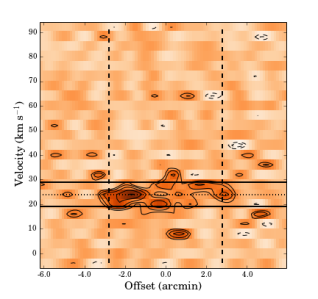
Figure 18: ALFALFA and WSRT data for AGC 249565 as in Figure 8 but with H i column density contours at [4, 6, 8, 10, 12.5, 15, 17.5] $\times 10^{18}$, [0.9, 1.5, 2, 2.5] $\times 10^{19}$, and [1.25, 1.5, 2, 2.5, 3.5] $\times 10^{19}$ atoms cm^-2 for the 210^′′, 105^′′, and 60^′′ data and velocity contours at [24, 26, 28, 30, 32] km s^-1.

Figure 1 shows the distribution of $S_{21}$, $W_{50}$, $\bar{a}$ and $N_{HI}$ for the UCHVC catalog of A13, including the most-isolated subsample, and the UCHVCs observed in this work. Generally, the UCHVCs observed here have a similar distribution of H i properties to those listed in the catalog of A13. The ALFALFA data are presented in Figures 8–19. The H i spectra are shown in the upper left panels, and the upper right panels show total intensity H i maps from ALFALFA in grayscale.

2.2 WSRT

The twelve UCHVCs were observed with WSRT over the course of two semesters under programs 13B-007 and 14A-017. The sources were observed using standard 13-hour synthesis imaging tracks consisting of 12 hours on source bracketed by half an hour on a standard calibrator. The sources were observed for a minimum of two tracks; a few sources were reobserved for a third track due to poor data quality in one of the original tracks. These observations occurred during the transition to the Apertif system and while the antennas were being refurbished. For the majority of observations, at least three antennas were out of the array for testing of Apertif prototypes, and, especially for the later observations, more antennas were often out of the array. Table 2 gives the noise value of the final data cubes for all the sources; the varying sensitivity of the different observations can be seen in the different noise values. The spectral setup of the observations was a 10 MHz bandwidth divided into 2048 channels, corresponding to a native resolution of 4.88 kHz, or $\sim$1 km s^-1.

Table 2: WSRT imaging parameters

HVC name	AGC	Taper			Restoring beam			rms	$\sigma_{N_{HI}}$
		Major	Minor	P.A.	Major	Minor	P.A.	$\Delta$v=4 km s-1	$\Delta$v=20 km s-1
		′′	′′	deg	′′	′′	deg	mJy bm-1	$10^{18}$ atoms cm-2
(1)	(2)	(3)			(4)			(5)	(6)
HVC214.78+42.45+47	198606	265	195	115	209.6	205.7	-43	1.9	0.4
		125	100	115	103.1	102.5	-35	1.6	1.5
		60	60	90	62.4	51.5	-166	1.4	4.3
HVC204.88+44.86+147	198511	240	185	105	204.9	200.8	76	2.0	0.5
		120	95	110	102.5	100.4	-26	1.5	1.4
HVC205.83+45.14+173	198683	245	185	105	206.9	204.4	57	2.1	0.5
		120	95	110	101.9	99.8	-31	1.6	1.6
HVC217.77+58.67+96	208747	255	185	110	208.4	204.9	-36	2.5	0.6
		120	95	110	100.0	99.2	-2	1.7	1.7
HVC212.68+62.39+64	208753	255	195	105	208.8	205.1	-36	2.5	0.6
		120	90	100	100.8	98.7	59	1.8	1.8
HVC230.27+71.10+76	219663	260	190	110	208.6	203.6	-43	3.3	0.8
		120	85	90	103.6	101.1	24	2.7	2.5
HVC235.38+74.79+195	219656	250	185	110	207.1	202.6	-15	2.3	0.5
		120	95	110	100.3	99.3	-4	1.8	1.8
HVC271.57+79.03+248	229326	250	190	110	206.4	202.7	55	2.3	0.5
		120	95	110	99.7	98.1	65	1.9	1.9
HVC276.53+79.84+255	229327	260	190	110	206.1	201.3	65	2.4	0.6
		120	90	110	102.1	99.6	-19	1.8	1.7
HVC028.09+71.87-142	249393	255	205	110	206.8	203.2	66	3.1	0.7
		120	95	110	103.1	102.0	-178	2.4	2.3
HVC011.76+67.89+60	249525	255	195	110	209.1	205.3	55	2.3	0.5
		120	95	110	101.7	99.5	-15	1.7	1.7
		60	60	90	63.2	53.9	13	1.4	4.1
HVC015.96+63.90+44	249565	265	200	115	208.5	203.5	86	3.5	0.8
		120	90	110	100.0	100.0	-50	2.1	2.1
		60	60	90	71.7	53.5	15	1.8	4.6

The data were reduced in Miriad following standard procedure (Sault et al. 1995). The data were flagged manually for radio frequency interference (RFI), and the bandpass and initial gain calibration used the standard calibrators. A continuum image of the target field was used for a phase-only self-calibration. Line-free channels were used to subtract the continuum emission in the uv-plane. A first-order polynomial was used for removing the continuum except for a few cases where a higher-order polynomial was justified.

Imaging of the data was done using the Common Astronomy Software Applications package (CASA, McMullin et al. 2007). A spectral resolution of 4 km s^-1 and a spectral range of 100 km s^-1 was used for all the sources. The spectral range was centered on the source except for a few objects close to Galactic emission in velocity space. Then, the center velocity was offset to avoid having channels dominated by Galactic H i and to provide more signal-free channels. Due to the low surface brightness nature of the UCHVCs, significant tapering was required to robustly detect emission. All the sources were tapered to resolutions comparable to that of Arecibo ($\sim 210$^′′) and about twice the angular resolution ($\sim$105^′′). In addition, the sources that were strongly detected at 105^′′ resolution were imaged with a 60^′′ taper applied. Table 2 lists the applied tapers and the resulting beams for each source.

Table 3: WSRT H i properties

HVC name	AGC	R.A.+Dec.	cz	$W_{50}$	$\theta_{hf}$	SHI			$N_{HI,peak}$
					210′′	210′′	105′′	60′′	210′′	105′′	60′′
		J2000	km s-1	km s-1	′	Jy km s-1			$10^{19}$ atoms cm-2
(1)	(2)	(3)	(4)	(5)	(6)	(7)			(8)
HVC214.78+42.45+47	198606	093002.8+163813	51	24	11.4	15.3	14.0	11.8	4.2	4.9	6.1
HVC204.88+44.86+147	198511	093017.2+241119	151	15	7.0	0.86	0.78	…	0.59	0.98	…
HVC205.83+45.14+173	198683	093212.8+233348	176	23	8.2	0.63	0.42	…	0.46	1.2	…
HVC217.77+58.67+96	208747	103710.0+203214	96	19	6.8	1.69	1.57	…	1.1	1.6	…
HVC212.68+62.39+64	208753	104931.8+235526	65	24	10.6	3.32	3.1	…	0.93	1.4	…
HVC230.27+71.10+76	219663	113422.1+201212	73	13	5.8	0.65	0.49	…	0.68	1.1	…
HVC235.38+74.79+195	219656	115123.7+203403	191	28	8.0	1.22	1.09	…	0.67	1.2	…
HVC271.57+79.03+248	229326	122735.5+173852	239	22	5.5	0.63	0.58	…	0.63	1.0	…
HVC276.53+79.84+255	229327	123223.6+175522	253	17	8.8	0.62	0.62	…	0.38	0.88	…
HVC028.09+71.87-142	249393	…	…	…	…	…	…	…	0.34	…	…
HVC011.76+67.89+60	249525	141752.7+173240	47	18	6.8	5.12	4.85	4.64	3.6	4.8	5.4
HVC015.96+63.90+44	249565	143556.3+170847	29	18	5.4	1.69	1.74	1.6	1.8	2.9	4.0

Since the UCHVCs are narrow in velocity extent, show only small amounts of velocity structure, and are generally low S/N, special care was taken in isolating the emission for cleaning. For each spatial resolution, a single clean mask was created and used for all channels with emission. This mask was constructed by making a single channel image using the central velocity and velocity extent from the ALFALFA H i spectrum. This single channel image was then iteratively cleaned until a final image was reached. This image was then smoothed to 300^′′, 210^′′, or 120^′′ resolution for the 210^′′, 105^′′, and 60^′′ data, and clipped at the 2-$\sigma$ level to define the extent of source emission. The channels of the data cube with emission were determined by examining the dirty cubes and using the ALFALFA spectra as a guide. The single channel image mask was then used to populate these channels to create a 3-D clean mask. The data were then cleaned deeply, to half the rms value, to minimize the impact of residual flux.

Moment zero (total H i intensity) maps were created over the range of channels identified as having emission, without any pre-applied masking. The velocity range used for constructing the moment zero maps is indicated in the spectra panel in Figures 8–19. The non-primary-beam-corrected map for the 210^′′ data in contours of significance is compared to the ALFALFA H i map in Figures 8–19. In all cases, the ALFALFA H i morphology is well matched to the WSRT H i morphology at the same resolution; when the ALFALFA data suggest structure in the H i morphology this is also seen in the WSRT data. The primary-beam-corrected total intensity H i maps in units of column density for all imaging resolutions are also presented in Figures 8–18. (AGC 249393 is a non-detection in the WSRT data and so only a partial presentation of the WSRT data is included in Figure 19.) Peak column density values from these maps are reported in Table 3.

The primary-beam-corrected moment zero maps were used to find the total H i line flux of the sources. Since the contribution of low level emission is important for low surface brightness objects, the moment zero maps were smoothed before defining the source extent to determine the flux density. The level of smoothing was the same as for the creation of the clean masks: 300^′′, 210^′′, and 120^′′ for the 210^′′, 105^′′, and 60^′′ data. The smoothed maps were clipped at the 3-$\sigma$ level to define the source extent; this mask can be seen in Figures 8–18. The emission within this region in the original resolution maps was summed to determine the integrated flux density. Generally the region used for calculating the integrated line flux is much more extended than the high significance emission. The WSRT spectra shown in Figures 8–18 are derived using the same mask applied to primary-beam-corrected data cubes. Table 3 gives the final line flux values for the source for all resolutions. Generally, the derived integrated line flux is the same at both the 210^′′ and 105^′′ resolution, and reasonably close to the single-dish ALFALFA value. We discuss this further in Section 3. We take the uncertainty on the flux to be 10%; this is dominated by uncertainty in determining the source extent.

For regions of significant emission ($>5\sigma$ in the 210^′′ total intensity H i map and $>3\sigma$ for the higher resolution maps), we created moment 1 and moment 2 maps, representing the velocity field and velocity dispersion. These maps are also shown in Figures 8–18, along with position-velocity slices at all resolutions derived using the CASA task impv. The angle of the slices was set to highlight structure, either in H i morphology or kinematics, and can be seen overlaid on top of the moment maps.

In addition, the effective half-flux radii of the sources were estimated by measuring the integrated flux density in increasing circular apertures until half the total WSRT H i line flux is enclosed. In many cases the source structure is elongated, and so this is a very crude measure and is reported without errors. However, it is still a useful metric for comparison to the ALFALFA H i size. The WSRT half-flux apertures are reported in Table 3 and shown on the grayscale ALFALFA maps in Figures 8–18 with the ALFALFA half-power ellipse and $\bar{a}$ shown for reference.

3 Comparison of ALFALFA and WSRT derived H i properties

Table 4: Comparison of ALFALFA and WSRT H i properties

HVC name	AGC	$\theta_{hf}/\bar{a}$	$S_{WSRT}/S_{ALFALFA}$		$N_{HI,WSRT}/\bar{N}_{HI}$
			210′′	105′′	210′′	105′′
(1)	(2)	(3)	(4)		(5)
HVC214.78+42.45+47	198606	0.9	0.9 (0.1)	0.8 (0.1)	0.8 (0.1)	1.0 (0.1)
HVC204.88+44.86+147	198511	1.0	1.2 (0.1)	1.1 (0.1)	0.9 (0.2)	1.5 (0.3)
HVC205.83+45.14+173	198683	0.8	0.7 (0.1)	0.5 (0.1)	1.3 (0.3)	3.3 (0.8)
HVC217.77+58.67+96	208747	0.6	0.6 (0.1)	0.6 (0.1)	1.1 (0.2)	1.6 (0.4)
HVC212.68+62.39+64	208753	0.8	0.8 (0.1)	0.8 (0.1)	0.9 (0.1)	1.3 (0.3)
HVC230.27+71.10+76	219663	0.8	0.9 (0.1)	0.7 (0.1)	1.1 (0.2)	1.7 (0.5)
HVC235.38+74.79+195	219656	1.1	1.4 (0.2)	1.2 (0.1)	1.0 (0.2)	1.7 (0.4)
HVC271.57+79.03+248	229326	0.7	0.8 (0.1)	0.8 (0.1)	1.1 (0.2)	1.8 (0.5)
HVC276.53+79.84+255	229327	0.8	0.7 (0.1)	0.7 (0.1)	1.2 (0.3)	2.7 (0.7)
HVC028.09+71.87-142	249393	…	…	…	1.2	…
HVC011.76+67.89+60	249525	0.8	0.8 (0.1)	0.8 (0.1)	0.9 (0.1)	1.2 (0.2)
HVC015.96+63.90+44	249565	0.7	1.0 (0.1)	1.0 (0.1)	1.3 (0.2)	2.1 (0.4)

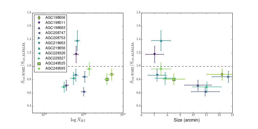
Figure 2: Fraction of ALFALFA flux recovered in the 210^′′ WSRT observations as a function of $\bar{N}_{HI}$ and size.

Table 4 lists the comparison of WSRT H i properties to the ALFALFA H i properties. The first thing to note is that the flux recovery is generally excellent (more than 50% in all cases) and there is generally very little change between the 210^′′ and 105^′′ WSRT data. This is due in large part to the expansive masks as a result of smoothing used for defining source extent. If the sources had been clipped directly on a threshold, the flux recovery would be much less, especially for the 105^′′ data as much of the flux is in low surface brightness emission that is on the level of the noise. Figures 8–18 illustrate this; the masks that define source extent are much broader than where the significant emission is located in most cases. Traditional wisdom says that interferometers miss flux because of the lack of short spacings but in many cases it may be an issue of lack of sensitivity to (or properly including) low column density emission rather than extended emission that is resolved out. Figure 2 shows the fraction of line flux recovered in the WSRT 210^′′ data relative to the ALFALFA data as a function of $\bar{N}_{HI}$ and size of the source. Generally, the sources with the highest peak column densities and the smallest sizes have the best flux recovery.

The left panel of Figure 3 shows that the ALFALFA $\bar{N}_{HI}$ value agrees extremely well with the WSRT 210^′′ peak $N_{HI}$, motivating the use of this average ALFALFA value. The right panel of Figure 3 also shows the peak $N_{HI}$ from the 105^′′ WSRT data compared to that from the 210^′′ data. All the sources have higher peak $N_{HI}$ at higher angular resolution as expected.

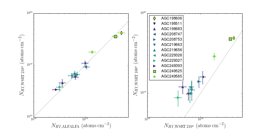
Figure 3: Left panel: ALFALFA $\bar{N}_{HI}$ versus the peak $N_{HI}$ from the 210^′′ WSRT data. Right panel: $N_{HI}$ at 105^′′ resolution compared to 210^′′.

Table 4 also lists the comparison of the effective half-flux size derived from the WSRT data to that from the ALFALFA data. While these sizes are in rough agreement, the sizes derived from the WSRT data tend to be smaller. That is consistent with the fact that WSRT data typically have smaller line flux values and the half-flux size is derived self-consistently for the WSRT data. Figures 8–19 also show that the H i morphology seen in the ALFALFA maps is matched by the morphology in the WSRT H i maps. When the ALFALFA data show elongated structure or evidence for multiple clumps, that structure is also seen in the WSRT H i data at the Arecibo resolution. Unfortunately, the reported parameters of the ALFALFA half-power ellipse, especially the position angle, do not always match the structure. This is consistent with what was seen in Adams (2014) where by measuring artificial sources it was shown that the average size of an UCHVC, $\bar{a}$, was an accurate measurement but that the measured ellipticity did not necessarily match the true ellipticity.

4 Discussion

4.1 The nature of the UCHVCs

The WSRT observations reveal that the UCHVCs fall into two categories: likely Galactic halo clouds and potential galaxy candidates. These two source populations are distinguished from each other based on a combination of H i morphology and kinematics. All the sources show a smooth H i morphology in the 210^′′ resolution data; this is consistent with their selection as UCHVCs from the ALFALFA data. The first set of sources, likely Galactic halo clouds, are distinguished by a lack of ordered velocity motion at all spatial resolutions and breaking into clumps of low column density H i contained in a much more diffuse envelope in the 105^′′ resolution data. This is consistent with previous observations of (compact) HVCs, and the likely explanation for these sources is that they are clouds of H i in the halo of the MW at typical distances of a 100 kpc (e.g., Brüns et al. 2001; de Heij et al. 2002; Westmeier et al. 2005b). In contrast, the potential galaxy candidates have ordered velocity motion at all angular resolutions and a smooth H i morphology in the 105^′′ resolution data. The potential galaxy candidates also have higher column density values, allowing them to be imaged at 60^′′ resolution, where they maintain the smooth H i morphology and ordered velocity motion. Figure 4 illustrates the comparison between the 210^′′ and 105^′′ resolution data for an example likely Galactic halo cloud and one of the potential galaxy candidates.

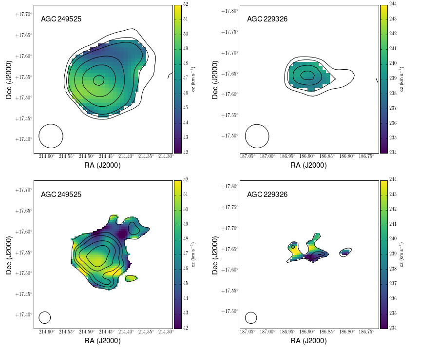
Figure 4: Velocity fields with H i column density contours of AGC 249525 (left) and AGC 229326 (right) at 210^′′ (top) and 105^′′ (bottom) resolution. AGC 249525 is representative of the potential galaxy candidates and AGC 229326 of the likely Galactic halo clouds. The column density contours for AGC 249525 for the 210^′′ and 105^′′ data are [4, 6, 8, 15, 25, 35] and [9, 15, 20, 30, 40] $\times 10^{18}$ atoms cm^-2. For AGC 229326 the column density levels are [2.5, 3.5, 5, 6] and [7, 9, 10] $\times 10^{18}$ atoms cm^-2.

The H i column density, velocity field, and velocity dispersion maps and the position-velocity slices used to determine the nature of the UCHVCs are presented in Appendix A. We determined that three sources are potential galaxy candidates. The remainder of the UCHVCs are considered likely Galactic halo clouds. The two sources from this work included in Bellazzini et al. (2015) and Sand et al. (2015), AGC 198511 and AGC 249393, show the morphology and lack of ordered velocity motion that is typical of Galactic halo clouds. This is consistent with the fact that these sources have no detected optical counterparts, down to strict limits (Beccari et al. 2016). AGC 198606 (also presented as a galaxy candidate in Adams et al. (2015)) and AGC 249525 are excellent galaxy candidates with a smooth H i morphology and evidence for ordered velocity motion at all spatial resolutions considered. AGC 249565 is a possible galaxy candidate, but the evidence for its ordered velocity motion is weaker, especially at higher angular resolution, and it may break into H i clumps in a more diffuse envelope in the 60^′′ resolution data, although this could be a S/N limitation. The ordered velocity motion is key for classifying a UCHVC as a galaxy candidate, and in Figure 5 we show the position-velocity slices for all three galaxy candidates to illustrate their ordered velocity motion.

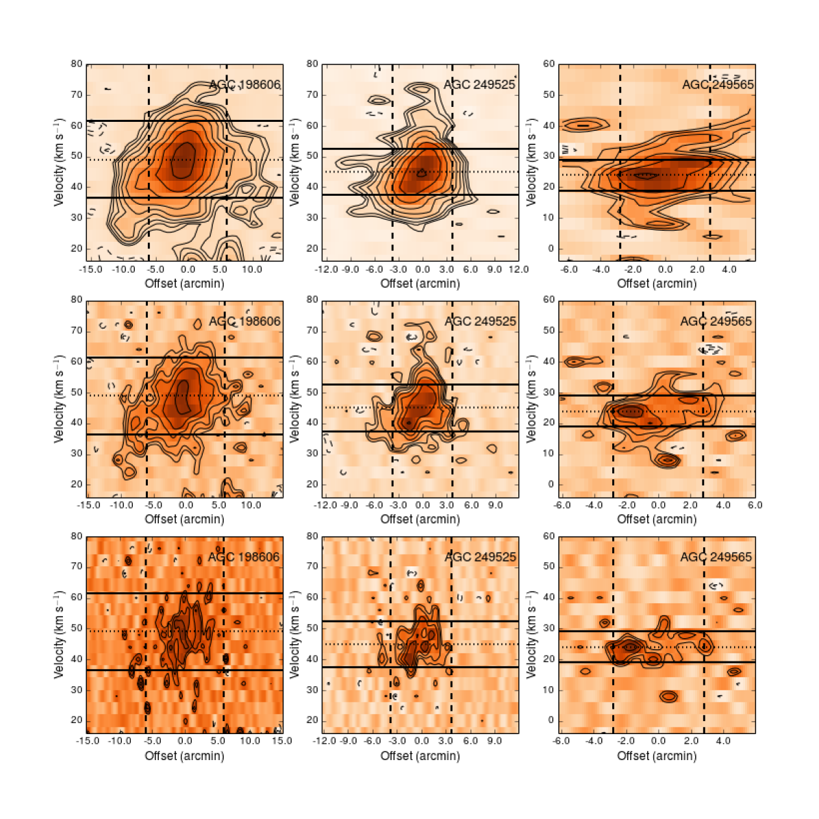
Figure 5: Position-velocity slices along the direction of ordered motion for the three galaxy candidates at 210^′′, 105^′′  and 60^′′ resolution (top to bottom). From left to right the sources are AGC 198606, AGC 249525, and AGC 249565. The contours start at 2 $\times$ rms of the data cube and increase by $\sqrt{2}$; negative contours with the same spacing are also shown. The solid horizontal black lines indicate the extent of velocity motion, and the dashed vertical lines indicate the spatial extent over which it occurs.

4.2 Identifying galaxy candidates

The goal of this work is to identify H i clouds that are good candidates to represent (nearly) starless gas in dark matter halos. In Section 4.1, we determined that AGC 198606 and AGC 249525 were excellent candidates to represent gas in dark matter halos while AGC 249565 was a potential third candidate. The majority of the UCHVCs (9/12) lack any kinematic structure and show a H i morphology at higher angular resolutions that is consistent with local Galactic halo clouds. This is not surprising as there are many potential formation mechanisms for HVCs and the majority of them are Galactic processes. An important step is to identify the H i properties by which the best galaxy candidates may be recognized. The targets were selected for WSRT observations on the basis of four criteria: isolation, compact size, large recessional velocity, or large average column density.

The three potential galaxy candidates were not selected for observations based on their size or isolation. While they are relatively compact and isolated, they are not distinguished from the rest of the UCHVC population by these two criteria. Instead, they are most clearly distinguished by having high column densities, as can be seen in Figure 3. In fact, the two best candidates, AGC 198606 and AGC 249525, have column densities higher than any source included in A13. While the peak column densities for these sources are higher than the other UCHVCs at all resolutions, their peak column density increases by less from the 210^′′ to 105^′′ data (right panel of Figure 3). This is consistent with their morphology in that the UCHVCs with the largest changes in peak column densities are those that show the most clumpiness at higher angular resolution.

Figure 6 shows the recessional velocities for all the candidates and the A13 sample in two different frames: helicoentric ($cz$), and Galactic standard of rest ($v_{GSR}$). Contrary to our expectations when selecting targets, the highest recessional velocity targets are not the best candidate galaxy candidates. Instead, the best candidates are those at low recessional velocity, with the three best candidates having $|v_{LSR}|<120$ km s^-1, outside the original selection selection criteria of A13. It is worth noting that Leo T has a low recessional velocity ($cz=35$ km s^-1), and we indicate its position in Figure 6. The picture that the best candidate galaxies are at low recessional velocities is consistent with theoretical work by Garrison-Kimmel et al. (2014). They find that never-accreted halos (the most likely to be overlooked gas-rich dwarf galaxies) in Local Group analogs are most likely to have radial velocities relative to their host galaxy with an amplitude $<$ 150 km s^-1 (e.g., $|v_{GSR}|<150$ km s^-1). This is in contrast to the work of Donovan Meyer et al. (2015) who find that H i clouds distinguished as velocity outliers are most likely to have a GALEX counterpart. However these are systems with apparent stellar counterparts and likely lie at larger distances within the Local Volume, rather than nearby in the Local Group.

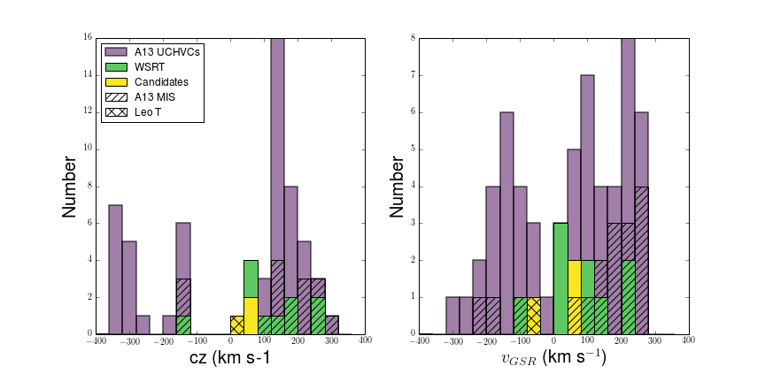
Figure 6: Distribution of velocities in heliocentric and Galactic standard of rest frames for the A13 UCHVCs and the UCHVCs of this work, with the good galaxy candidates highlighted in yellow.

Overall, the clearest distinguishing feature of the best galaxy candidates is their high column density (albeit still low for galaxies). They also tend to be small, isolated and at low velocity, but none of those criteria are sufficient to identify the best candidates. The fact that the best candidates are at low recessional velocities means that identifying these sources will be strongly complicated by the presence of the Galactic H i foreground.

4.3 Properties of galaxy candidates

In this section, we assume AGC 198606, AGC 249525, and AGC 249565 do in fact represent gas in dark matter halos and examine what their properties would be.

The strongest evidence that these three systems potentially represent gas in dark matter halos is the ordered velocity motion, which can be interpreted as rotation of the gas. The extent of this velocity motion is indicated in the position-velocity slices in Figure 5 and is in total 25, 15, and 10 km s^-1 for AGC 198606, AGC 259525, and AGC 249565. The magnitude of the velocity motion was determined to represent the global bulk velocity of the gas; gas exists at velocities beyond the extents indicated in Figure 5 due to the dispersion of the gas about the global bulk velocity.

In order to interpret the bulk velocity motion as a rotation velocity, the inclination of the system must be taken into account. For each candidate, a column density level at which the velocity motion could be reliably traced in both the 210^′′ and 105^′′ data was empirically determined. This physical extent is shown in Figure 5 by the vertical dashed lines. Due to lower sensitivity to low column density emission, the 60^′′ data typically does not trace the velocity motion to the same spatial extent as the 210^′′ and 105^′′ data. The axial ratio of each system was found by fitting an ellipse at this spatial extent to both the 105^′′ and 210^′′ data. For converting to an inclination, these systems are assumed to be thick disks with an intrinsic axial ratio of 0.6 (Roychowdhury et al. 2010); changing the assumed intrinsic axial ratio by 10% changes the derived inclination angles by a similar amount. For AGC 198606, the velocity motion is reliably traced to the $2\times 10^{19}$ atoms cm^-2 level. The fitted ellipse has a major axis of 12^′ $\pm$ 1^′ and the axial ratio is 0.75, which corresponds to an inclination of 56^∘. The corresponding rotation velocity is $15^{+4}_{-1}$ km s^-1, where the errors correspond to a 10% uncertainty on the axial ratio. For AGC 249525 the $1.5\times 10^{19}$ atoms cm^-2 level was used, which has a major axis of 7.5^′ $\pm$ 0.1^′ and an axial ratio of 0.91, corresponding to an inclination of 30^∘. Then the rotation velocity is 15${}_{-2}^{+6}$ km s^-1. And for AGC 249565 the extent of the velocity motion was seen to the $1\times 10^{19}$ atoms cm^-2 level. This source shows the very unusual behavior that it has a larger major axis at this level in the 105^′′ data than the 210^′′ data. We take the major axis of 5.6^′ $\pm$ 0.1^′ from the 210^′′ data as the extent for this source. The axial ratio is 0.86 and the rotation velocity is 8${}^{+4}_{-2}$ km s^-1. The accuracy of these values is limited by the determination of the velocity extent, assumption that the velocity gradient represents rotation, and the assumed inclination of the system. This is particularly problematic for AGC 249525 as its axial ratio is close to unity and small changes in the fitted axial ratio greatly impact the final rotation velocity. These velocity values are comparable to those seen in other low mass dwarf galaxies, such as Leo P, Pisces A and B, and the SHIELD galaxies (Bernstein-Cooper et al. 2014; Carignan et al. 2016; McNichols et al. 2016).

These rotation velocities can be used to constrain the dynamical mass of the systems. These systems have low rotation velocities, on the order of their velocity dispersion. Thus, we follow Hoffman et al. (1996) and explicitly include the dynamical support of velocity dispersion of the gas when calculating the dynamical mass within a given radius:

$$M_{dyn}=2.325\times 10^{5}\,M_{\odot}\,\frac{V_{rot}^{2}+3\sigma_{z}^{2}}{\mathrm{km^{2}\,s^{-2}}}\,\Bigg{(}\frac{r}{\mathrm{kpc}}\Bigg{)}.$$ (2)

We take representative velocity dispersion values from the moment two maps. For AGC 198606 this is 9 km s^-1, and for AGC 249525 and AGC 249565 this is 7 km s^-1.

In order to calculate the dynamical mass or understand any of the other intrinsic properties of these systems, a distance is necessary. The most straight-forward way to obtain a distance is to detect a stellar counterpart. All three of these systems lie out side the $\alpha.40$ footprint and so are not considered in the works of Bellazzini et al. (2015) and Sand et al. (2015). In Adams et al. (2015) we argued that due to its small separation in position and velocity space from Leo T that AGC 198606 is likely located at a similar distance. In subsequent work, Janesh et al. (2015) found a tentative stellar counterpart (92% confidence) at a distance of 383 kpc, consistent with AGC 189606 being physically associated with Leo T. Using the slightly higher H i integrated flux density value of this work, the H i mass at a distance of 383 kpc is $5.3\times 10^{5}$ $M_{\odot}$, and the system is extremely H i dominated, with $M_{\mathrm{HI}}$/$M_{*}$$>50$.

We can use a similar philosophy to try and constrain the distances to AGC 249525 and AGC 249565. These two sources are located 4.3^∘ from each other so we consider their potential neighbors together. Within 10^∘ and 200 km s^-1 there are three galaxies: Bootes I at distance of 66 kpc (Dall’Ora et al. 2006), Bootes II at a distance of 46 kpc (Koch et al. 2009), and UGC 9128 at a distance of 2.27 Mpc (Tully et al. 2013). Given the observed morphological segregation in the Local Group (Spekkens et al. 2014), these systems are unlikely to be associated with Bootes I and II, but could be associated with UGC 9128. Thus we can adopt 2 Mpc as a representative upper distance for these two sources. As a representative lower distance, we take 0.4 Mpc, the distance of Leo T and AGC 198606.

Table 5: Properties of galaxy candidates

Name	Distance	$M_{\mathrm{HI}}$	$v_{rot}$	$r_{HI}$	$M_{dyn}$	$M_{\mathrm{HI}}$/$M_{dyn}$
	Mpc	$10^{5}$ $M_{\odot}$	km s-1	kpc	$10^{7}$ $M_{\odot}$
(1)	(2)	(3)	(4)	(5)	(6)	(7)
AGC 198606	0.383	$5.3$	15${}^{+4}_{-1}$	0.66	$7$	0.008
AGC 249525	$0.4-2$	$1.9-48$	15${}^{+6}_{-2}$	0.44 –2.2	$4-20$	$0.005-0.02$
AGC 249565	$0.4-2$	$0.64-16$	8${}^{+4}_{-2}$	0.33 – 1.6	$2-8$	$0.003-0.02$
Leo T	0.42	2.8	–	0.3	0.33	0.085
Leo P	1.62	8.1	15	0.5	2.5	0.032

Table 5 summarizes the properties of these sources for the relevant distances, with Leo T and Leo P given for reference. AGC 198606 is physically bigger than Leo T and Leo P (albeit measured at a much lower column density level) while its H i mass is intermediate between the two galaxies. Its rotational velocity is similar to that of Leo P but its dynamical mass is larger due to its larger physical size. AGC 249525 has an H i mass slightly smaller than Leo T and an H i size between that of Leo T and Leo P at the lower bound of the distance range considered for it. Its rotational velocity is comparable to Leo P and it has a similar dynamical mass. At the upper end of the distance range considered, AGC 249525 is much larger than Leo T and Leo P in terms of H i mass, H i size, and dynamical mass. At its closest plausible distance, AGC 249565 has a quarter of the H i mass of Leo T but a similar H i size. At its furthest considered distance, AGC 249525 has twice the H i mass of Leo P and three times the H i extent.

These three candidate galaxies are distinguished from Leo T, Leo P and other low mass galaxies by the extremes of their baryonic component: they have a minimal stellar component, are extremely dark matter dominated, and have extremely low peak column densities. AGC 198606 has a tentative stellar component with a mass of only $\sim 10^{4}$ $M_{\odot}$ (Janesh et al. 2015); AGC 249525 and AGC 249565 have no known stellar counterpart. For all distances considered for AGC 198606, AGC 249525 and AGC 249565, they are extremely dark matter dominated objects, with $M_{\mathrm{HI}}$/$M_{dyn}$$\leq$ 0.02 in all cases. This is lower than the $M_{\mathrm{HI}}$/$M_{dyn}$ value of Leo P, where the stellar population also contributes significantly to the total baryon mass ($M_{bary}$/$M_{dyn}$$=$ 0.05). The peak column densities of these three candidates with a 60^′′ beam (0.1 kpc at 400 kpc or 0.6 kpc at 2 Mpc) are $4-6\times 10^{19}$ atoms cm^-2. The least resolved SHIELD galaxies have a physical resolution of $\sim 0.6$ kpc but their peak column densities are almost an order of magnitude higher (Teich et al. 2016).

The left panel of Figure 7 places these three candidate galaxies in the context of the baryonic Tully-Fisher relation (BTFR), a tight observed correlation between the baryonic mass of a galaxy and its maximum rotational velocity. We show the relation of McGaugh (2012) along with the galaxies used in that work. We also include the SHIELD galaxies and Leo P for an extension to lower masses (Bernstein-Cooper et al. 2014; McNichols et al. 2016). The three candidate galaxies of this work are placed on this relation using the rotation velocities derived in this work and with baryonic masses consisting of only a neutral gas component (the H i mass multiplied by a 1.33 correction factor to account for Helium). For AGC 198606 we use the distance from Janesh et al. (2015) of $383\pm 10$ kpc and include the uncertainty in the neutral gas mass of 10% (based on the uncertainty of the WSRT integrated flux) in the vertical error bars; the potential stellar component is neglected as it negligible compared to the gas mass. For AGC 249525 and AGC 249565, we use a representative distance of 1 Mpc and the vertical errors bars indicate the range of distances considered, $0.4-2$ Mpc. These three candidate galaxies are consistent with extending the BTFR to lower rotation velocities. AGC 198606 and AGC 249525 occupy the same region as Leo P and AGC 249565 extends the relation to even lower rotation velocities.

In order to test the significance of the three candidate galaxies lying on the BTFR, in the right panel of Figure 7 we place all the UCHVCs on the BTFR based on their single-dish ALFALFA H i properties. The baryonic mass is the H i mass for an assumed distance of 1 Mpc multiplied by a correction factor of 1.33 to account for Helium, and $v_{rot}$ is approximated as $\sqrt{3}\sigma$, where $\sigma$ is the line-of-sight velocity dispersion of the gas based on the $W_{50}$ value. The general UCHVC population occupies a region of parameter space below the BTFR. Interestingly, the candidate galaxies are among the sources that scatter closest the BTFR based on single-dish properties.

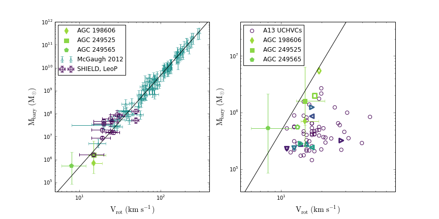
Figure 7: Left: AGC 198606, AGC 249525 and AGC 249565 (the three galaxy candidates) shown on the Baryonic Tully-Fisher relation (BTFR) of McGaugh (2012) with Leo P and the SHIELD galaxies (Bernstein-Cooper et al. 2014; McNichols et al. 2016) shown for extension to low rotational velocities. Right: UCHVCs of A13 (open circles) and this work (open symbols, same colors and shapes as in Figures 2 and 3) shown on the BTFR based on their single-dish ALFALFA properties. The galaxy candidates are shown based on their rotation velocities derived in this work.

4.4 Implications for future surveys

In line with previous work, these observations highlight the power of resolved H i observations for addressing questions as to the nature of (ultra-) compact HVCs and whether they can represent gas in dark matter halos (e.g., de Heij et al. 2002; Brüns & Westmeier 2004; Westmeier et al. 2005b, a). Of the twelve clouds identified in the single-dish ALFALFA survey, the higher angular resolution WSRT observations show that only three of the objects are potential candidates to represent gas in dark matter halos. With future large-field surveys planned with interferometers (e.g., Apertif and ASKAP), many more of these objects will be detected and immediately distinguished as galaxy candidates. If AGC 198606, AGC 249525, and AGC 249565 do indeed represent what we might expect for gas-rich (nearly) starless galaxies in the Local Universe, we can use them as guides for how to find more of these objects in future surveys. Importantly, while they are the highest column density objects studied here, their peak column densities are lower than that typically found in low mass galaxies by an order of magnitude. In order to robustly detect and image these objects in future surveys, a special handling of the data with strong angular smoothing will be called for.

5 Summary

We present WSRT H i observations of twelve UCHVCs identified in the ALFALFA H i survey as good candidates to be gas-bearing dark matter halos. Our key results are as follows:

• The flux recovery from the WSRT observations compared to the ALFALFA data is generally excellent. This is due to the use of a smoothed image to define the source extent to ensure that low column density emission on the level of the noise is included in the calculation of the integrated line flux.

• Two of the twelve UCHVCs, AGC 198606 and AGC 249525, are excellent candidates to represent gas in dark matter halos. A third UCHVC, AGC 249565, is a possible candidate. The property that most distinguishes the galaxy candidates from the rest of the UCHVC population is having a higher average column density in the ALFALFA H i data.

• In addition, the best galaxy candidates have low recessional velocities. This is consistent with theoretical predictions for the Local Group, but means identifying the best candidates will be challenging as they must be distinguished from the Galactic H i foreground.

• AGC 198606 is an excellent galaxy candidate, as discussed previously in Adams et al. (2015) and Janesh et al. (2015). Based on the H i properties derived in this work, and the distance of Janesh et al. (2015), we find it has an H i mass of $5.3\times 10^{5}$ $M_{\odot}$, a rotational velocity of $15^{+4}_{-1}$ km s^-1, a radius of 0.66 kpc, and a dynamical mass of $7\times 10^{7}$ $M_{\odot}$.

• AGC 249525 is the other best galaxy candidate. It has a rotation velocity of $15^{+6}_{-2}$ km s^-1, and for the plausible range of distances $0.4-2$ Mpc, it has an H i mass of $1.9-48\times 10^{5}$ $M_{\odot}$, an H i radius of $0.44-2.2$ kpc, and a dynamical mass of $4-20\times 10^{7}$ $M_{\odot}$.

• AGC 249565 is the third potential galaxy candidate, although we emphasize it is much less likely to represent gas in a dark matter halo than the other two. This source has a rotation velocity of $8^{+4}_{-2}$. For the assumed distance range of $0.4-2$ Mpc, it has an H i mass of $0.64-16\times 10^{5}$ $M_{\odot}$, an H i radius of $0.33-1.6$ kpc, and a dynamical mass of $2-8\times 10^{7}$$M_{\odot}$.

• Future H i surveys with interferometers will be able to distinguish galaxy candidates immediately on the basis of H i morphology and kinematics but must make sure that the data handling allows for for sensitivity to low column density emission.

Appendix A Presentation of the H i data

Here we present the ALFALFA and WSRT data for each UCHVC, along with a brief discussion of the source and results of the WSRT observations. Figures 8–19 present the WSRT and ALFALFA H i data for each source in a consistent manner. The left figure in the first row shows the spectra for the primary-beam corrected WSRT data (at all resolutions imaged), and the ALFALFA spectrum. The bottom panel of this figure shows a representative noise spectrum from a signal-free portion of the (non-primary-beam-corrected) WSRT data cubes. The right panel in the first row is an ALFALFA grayscale map with the (non-primary-beam-corrected) WSRT 210^′′ moment zero map overlaid in units of significance, and the ALFALFA and WSRT effective half-flux apertures shown. The following rows present the WSRT data at all relevant angular resolutions. The left panel is (primary beam corrected) H i column density contours overlaid on the moment one (velocity field) map, the center panel is the moment two (velocity dispersion) map with lines of constant velocity overlaid, and the right panel is the position-velocity slice, along the direction shown in the two left panels.

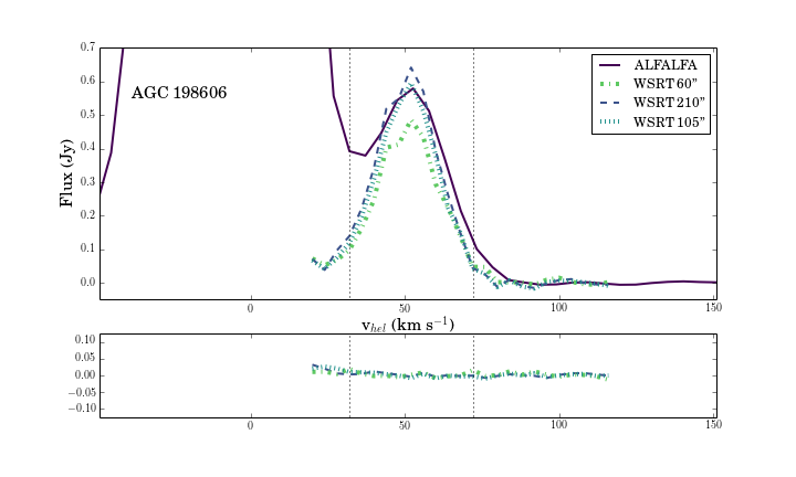
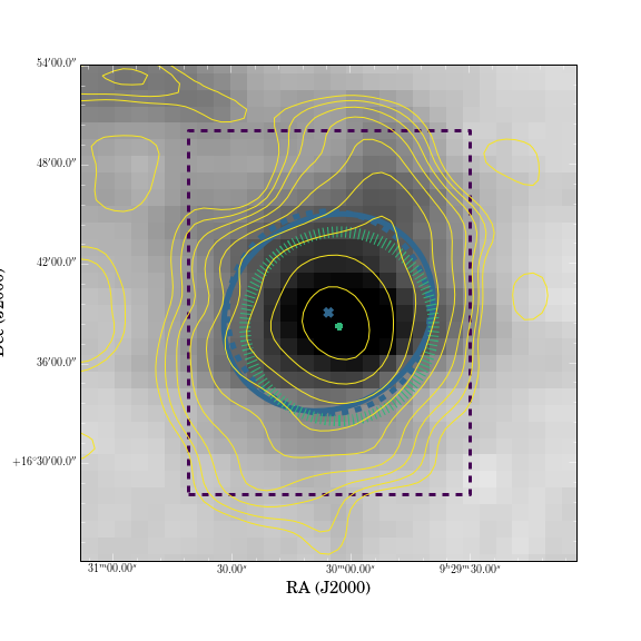
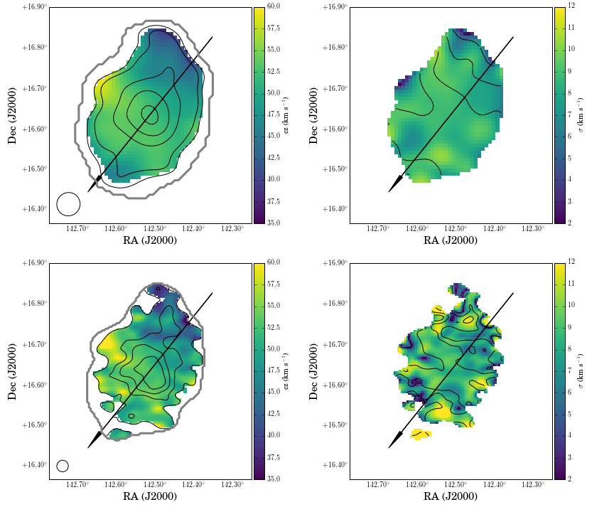
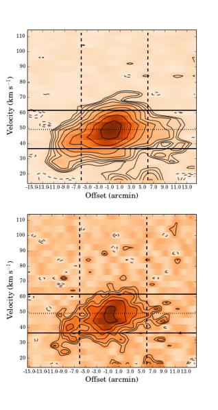
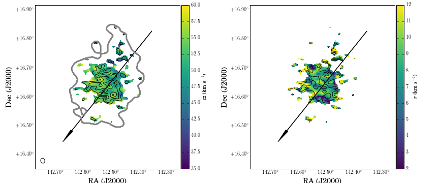
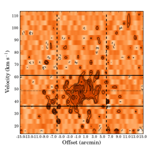
Figure 8: ALFALFA and WSRT data for AGC 198606. Top, left: Spectra for the source: solid purple is the ALFALFA spectrum, dashed blue-purple the 210^′′ WSRT spectrum, dotted blue the 105^′′ WSRT spectrum, and the dashed-dotted green the 60^′′ WSRT spectrum. The light dotted black lines indicate the velocity range used for creation of the WSRT moment maps. The bottom panel shows the noise from a representative region of the WSRT data cube. Top, right: The ALFALFA total intensity H i map in grayscale with the region used for source measurement highlighted by the dashed rectangle. The yellow contours are the WSRT 210^′′ moment zero map contours starting from 2 $\times$ rms and increasing by $\sqrt{2}$; dashed negative contours with the same spacing are also shown. The blue ellipse represents the ALFALFA fitted ellipse and the dashed blue circle the equivalent $\bar{a}$, average angular size. The dotted green circle represents the effective half-flux aperture derived in this work. Bottom: The WSRT H i data. From left to right, the panels show the velocity field with column density contours overlaid (and the mask used to extract the integrated flux density and spectrum in dark gray), the velocity dispersion map with lines of constant velocity from the velocity field, and a position velocity slice along the arrow shown in the left and central panels. The H i column density contours for the three resolutions are [0.7,1, 2, 3, 4] $\times 10^{19}$, [1, 2, 3, 4, 5] $\times 10^{19}$ and [3, 4, 5, 6] $\times 10^{19}$ atoms cm^-2. The constant velocity contours are [42, 46, 50, 54, 60] km s^-1. Contours for the position-velocity slice start at 2 $\times$ rms of the data cube and increase by $\sqrt{2}$; negative contours with the same spacing are also shown.

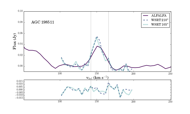
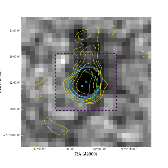
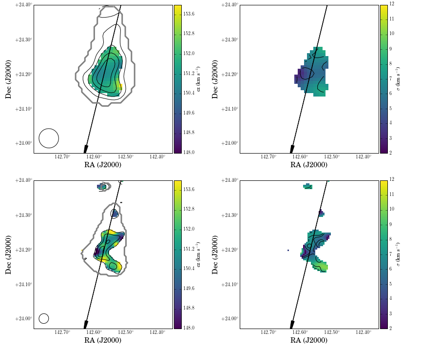
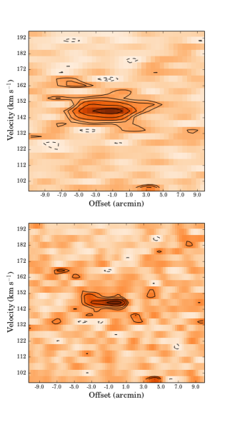
Figure 9: ALFALFA and WSRT data for AGC 198511 as in Figure 8 but with H i column density contours at [2, 3, 4, 5] $\times 10^{18}$ and [5, 7, 9, 12.5] $\times 10^{18}$ atoms cm^-2 for the 210^′′ and 105^′′ data and velocity contours at [151, 152] km s^-1.

AGC 198606: This source was chosen for observation because of its proximity to the gas-rich ultra-faint dwarf galaxy Leo T and similar H i properties within the ALFALFA H i dataset. WSRT observations of this source were also presented in Adams et al. (2015). The images here represent a reprocessing of the same data with an additional (heavily flagged) track included. Figure 8 presents the H i data for AGC 198606. The source is among the most extended of the UCHVCs observed with WSRT, but it has a smooth H i morphology at both the Arecibo and 105^′′ resolution, as seen in Figure 8, and thus it was also imaged with a 60^′′ taper. This source overlaps with the foreground Galactic H i in velocity-space, and special care is needed to needed to isolate the emission of the source from the foreground. For example, the ALFALFA source box seen in Figure 8 does not encompass all of the significant emission seen in the WSRT contours; this is because the presence of the Galactic H i foreground made it difficult to determine the physical extent of AGC 198606 in the ALFALFA data. The difficultly with the Galactic H i is also seen in the WSRT data; the apparent turn-over in the velocity gradient seen on the south-eastern edge of the 210^′′ velocity field is likely caused by Galactic H i entering the source mask. As discussed in Adams et al. (2015), the velocity fields and position velocity slices of this source at both 210^′′ and 105^′′ resolution show ordered motion with a gradient of $\sim 25$ km s^-1. In this work we see that this velocity motion is also present in the higher angular resolutions 60^′′ data. This range of velocity motion, along with the spatial extent at which it is seen at all resolutions, is indicated in the position-velocity slices in Figures 8 and 5. The interpretation of this velocity gradient is discussed in Section 4.3. We also note that the integrated flux derived here is slightly higher than that in Adams et al. (2015), although still consistent within the errors. This demonstrates the sensitivity of the final integrated line flux to the exact source extent.

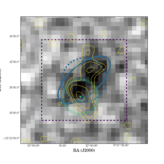
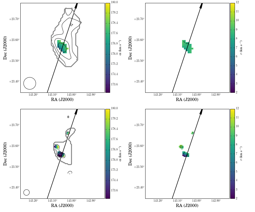
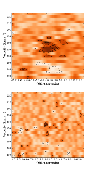
Figure 10: ALFALFA and WSRT data for AGC 198683 as in Figure 8 but with H i column density contours at [2, 3, 4] $\times 10^{18}$ and [6, 8, 10] $\times 10^{18}$ atoms cm^-2 for the 210^′′ and 105^′′ data and velocity contours at [175, 178, 181] km s^-1.

AGC 198511: This source is included in the most-isolated subsample of A13 and was selected for WSRT observations because of its isolation; it is also one of the most compact sources. Figure 9 presents the H i data for this source. At the Arecibo resolution, this source has a smooth H i distribution, elongated to the North. This elongation is also seen in the ALFALFA total intensity H i map. In addition, both the WSRT and ALFALFA data show that this elongation connects to another (lower intensity) clump of emission. At higher angular resolution, the main body of the source consists of separate clumps in an envelope with a morphology reminiscent of ram pressure effects. Neither the velocity field nor the position-velocity slice show any strong evidence for ordered velocity motion. Generally this source has a small velocity dispersion. The source extent for the WSRT data at 210^′′ resolution includes some of the northern extension, which was not included in the source box for the ALFALFA data, thus explaining a slightly higher integrated flux density for the WSRT 210^′′ data than the ALFALFA data.

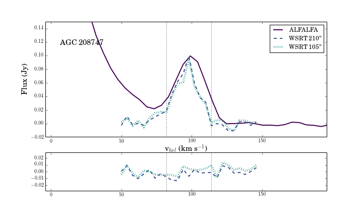
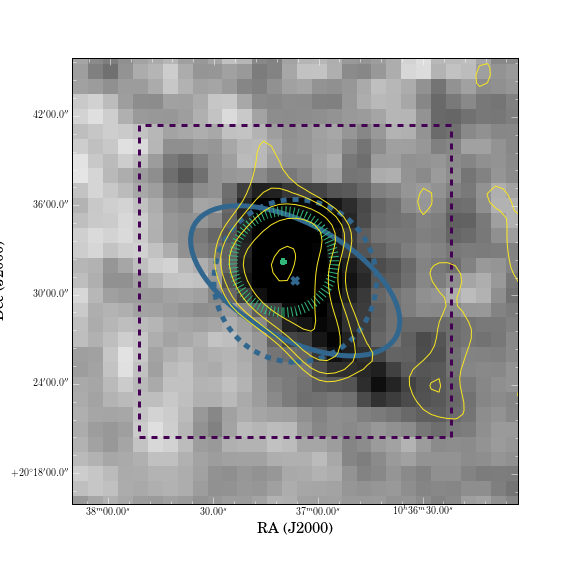
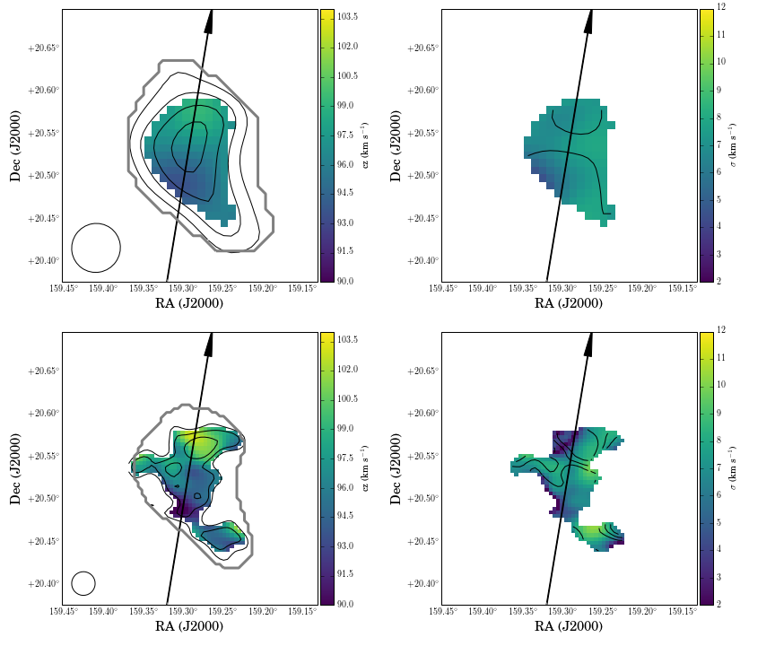
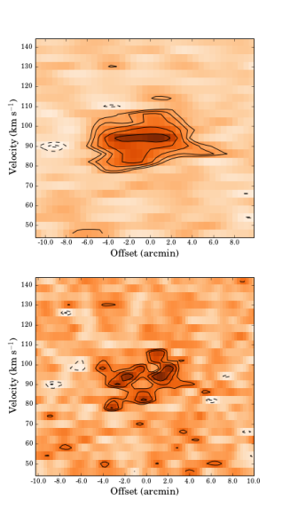
Figure 11: ALFALFA and WSRT data for AGC 208747 as in Figure 8 but with H i column density contours at [4, 6, 8,10] $\times 10^{18}$ and [8, 10, 12.5] $\times 10^{18}$ atoms cm^-2 for the 210^′′ and 105^′′ data and velocity contours at [96, 98, 100] km s^-1.

AGC 198683: This source was also selected for its isolation; it is relatively close to AGC 198511 but it is larger and has a lower column density in the ALFALFA H i data, making it a less promising candidate. The H i data for this source are presented in Figure 10. The WSRT data quality for this source is relatively poor, as can be seen in the noisy spectra. At the 210^′′ resolution, the source shows elongation to the north, which is aligned with the extension seen in the ALFALFA grayscale map. This structure is also reflected in the ALFALFA half-power ellipse. At higher angular resolution, the main body of source emission resolves into two clumps while the northern clump is also detected. Only a fraction of the ALFALFA flux is detected, indicating that much of the emission is low surface brightness and extends further than the flux masks indicate. This is consistent with less flux being recovered in the 105^′′ data which is less sensitive to low column density emission. The source has no velocity structure.

AGC 208747: This source was selected for having a high average column density value from the ALFALFA data. Figure 11 presents the H i data for AGC 208747. At ALFALFA resolutions, the source is smooth and slightly elongated. At higher angular resolutions, the main body shows some clumpiness but is generally smooth. The tail separates into a separate clump of emission, connected by low level emission to the main body. The velocity fields appear to indicate a potential velocity gradient across the source, but there is no evidence for ordered velocity motion in the position-velocity slices. The WSRT data match the blue end of the ALFALFA spectrum well but are missing emission on the red end.

AGC 208753: This source was chosen based on isolation and a high average column density value from the ALFALFA data. The H i data for AGC 208753 are presented in Figure 12. At the ALFALFA resolution it is elongated in the north-south direction and consists of two separate clumps connected at the level of $5\times 10^{18}$ atoms cm^-2. This structure is tentatively seen in the ALFALFA grayscale map, although the position angle of the ALFALFA half-power ellipse is perpendicular to the elongation. At higher angular resolution, this source breaks into multiple clumps, in a common envelope around $5\times 10^{18}$ atoms cm^-2. No velocity structure is evident in the velocity field or position velocity slices. The clumpy nature of this source at higher angular resolution is also seen in the position-velocity slice. The ALFALFA flux is well recovered by both the 210^′′ and 105^′′ data.

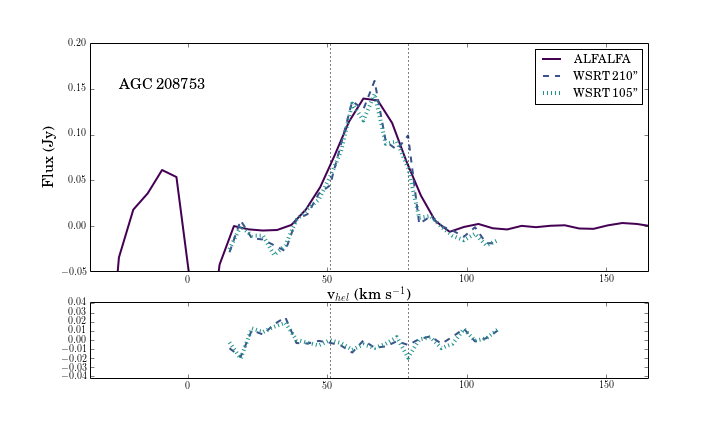
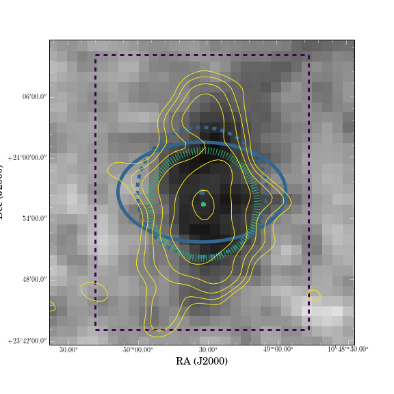
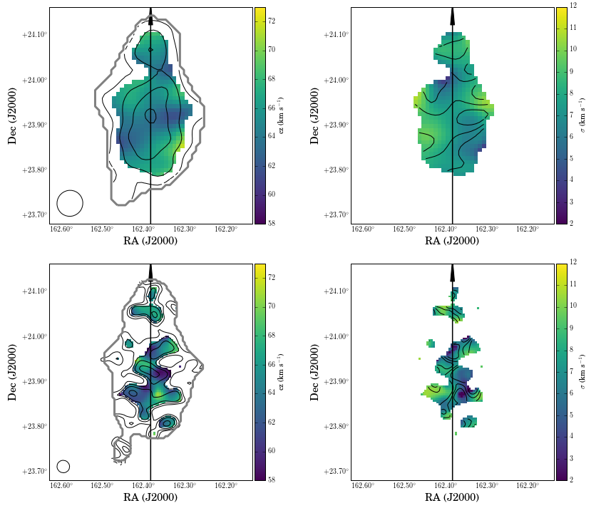
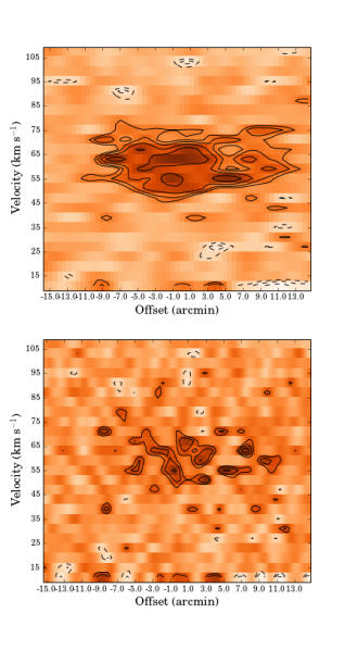
Figure 12: ALFALFA and WSRT data for AGC 208753 as in Figure 8 but with H i column density contours at [3, 5, 7, 9] $\times 10^{18}$ and [5, 7, 9, 12.5] $\times 10^{18}$ atoms cm^-2 for the 210^′′ and 105^′′ data and velocity contours at [63, 65, 67] km s^-1.

AGC 219663: This object was selected for its compact size. Figure 13 presents the H i data for AGC 219663. At the ALFALFA resolution, this source shows very little structure but does have a hint of elongation to the north-east. This elongation is also seen in the ALFALFA grayscale map and in the position and orientation of the ALFALFA half-power ellipse. The source has very little velocity structure; there is an apparent gradient in the velocity field but it is only of order $\sim 5$ km s^-1, and in the position-velocity diagram there appears to be two separate velocity structures. The source has low velocity dispersions across the entire extent of emission. At higher angular resolution, the source appears as two clumps that are barely detected. These appear to be the two separate velocity structures hinted at in the 210^′′ data; this is also seen in the position-velocity slice. The total integrated flux density recovered is slightly lower than the ALFALFA value, although the emission detected in the WSRT cubes appears at the 210^′′ resolution appears to be narrower in velocity width than that of the ALFALFA data, as seen in the spectra figure.

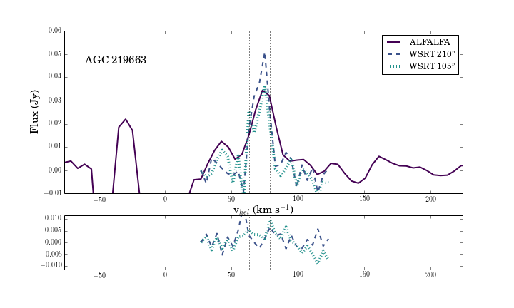
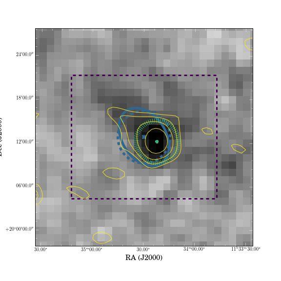
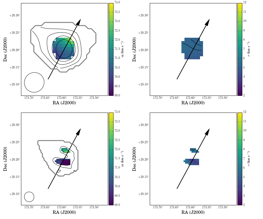
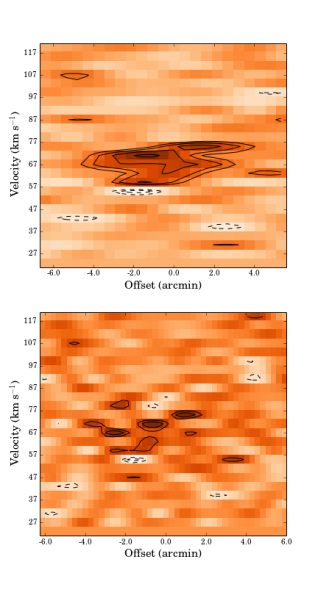
Figure 13: ALFALFA and WSRT data for AGC 219663 as in Figure 8 but with H i column density contours at [2.5, 3.5, 4.5, 5.5] $\times 10^{18}$ and [7, 9] $\times 10^{18}$ atoms cm^-2 for the 210^′′ and 105^′′ data and velocity contours at [71,72] km s^-1.

AGC 2196565: This UCHVC was selected for its fairly compact H i size and isolation in that ALFALFA data. The H i data are shown in Figure 14. At the ALFALFA resolution, it is extended in the northeast-southwest direction; evidence for this elongation is also seen in the ALFALFA map. The WSRT data also show a secondary structure, perpendicular to the main axis. This is not obviously evident in the ALFALFA data. At higher angular resolution, the source breaks into multiple clumps along the axis of elongation, and there are are also two separate clumps associated with the perpendicular structure. There is no clear velocity structure in the source, in either the velocity fields or position-velocity slices. We note that this source has a higher measured integrated flux density from the WSRT data than the ALFALFA data. There is no clear explanation for this as the ALFALFA source box encompasses all of the WSRT emission and this object is well removed from the Galactic foreground in velocity space. The perpendicular structure is not seen in the ALFALFA data and the inclusion of it in the WSRT maps may account for the larger recovered flux. As can been seen in the bottom of the spectra panel in Figure 14, the noise levels for this source are high, and it is possible that this extra structure is a left-over imaging artifact.

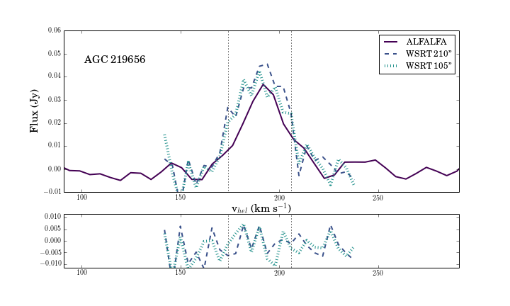
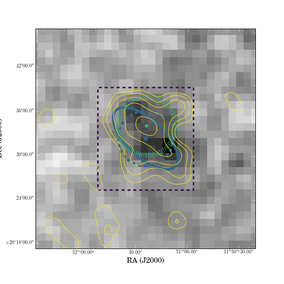
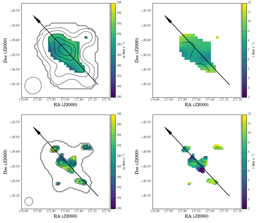
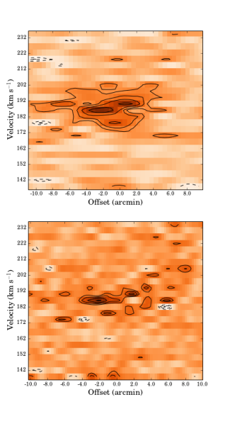
Figure 14: ALFALFA and WSRT data for AGC 219656 as in Figure 8 but with H i column density contours at [2, 3, 4, 5, 6] $\times 10^{18}$ and [7, 9, 10] $\times 10^{18}$ atoms cm^-2 for the 210^′′ and 105^′′ data and velocity contours at [185, 190] km s^-1.

AGC 229326: This source was selected for observation because of its relatively high recessional velocity, typically difficult to explain in Galactic fountain models of high velocity clouds. Figure 15 presents the WSRT and ALFALFA H i data. At the Arecibo resolution, this source is compact with a slightly extended H i tail. At higher angular resolutions, the source breaks into three distinct clumps, with one of these in the tail seen at lower resolution. As seen in the position-velocity slices, AGC 229326 appears to consist of clumps of emission with narrow velocity widths. The WSRT spectra lack emission on the red end compared to the ALFALFA spectrum. This is a low S/N detection in the WSRT data, as evident in the noise in both the spectra and position-velocity slices.

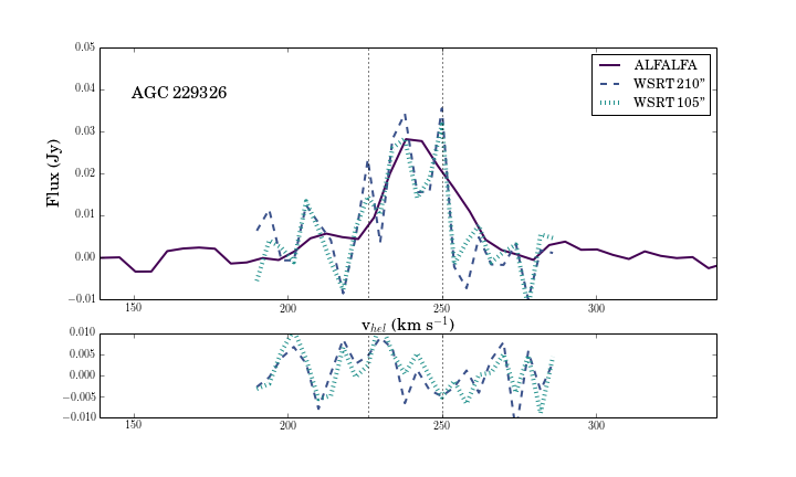
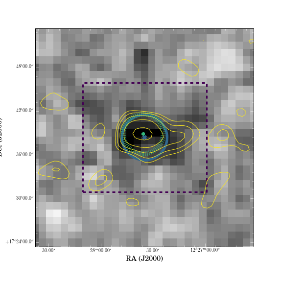
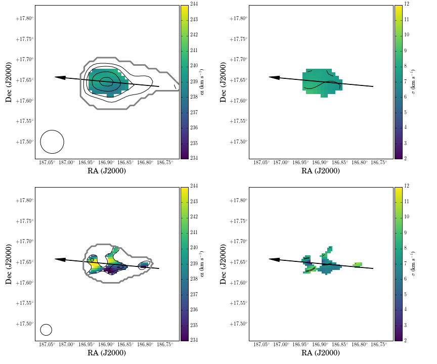
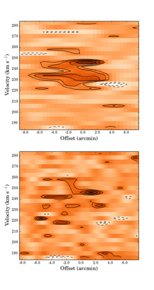
Figure 15: ALFALFA and WSRT data for AGC 229326 as in Figure 8 but with H i column density contours at [2.5, 3.5, 5, 6] $\times 10^{18}$ and [7, 9, 10] $\times 10^{18}$ atoms cm^-2 for the 210^′′ and 105^′′ data and constant velocity contours at [239, 240] km s^-1.

AGC 229327: This object was chosen for its high recessional velocity, although it is also among the largest and lowest surface brightness of the ALFALFA UCHVCs targeted for follow-up. Figure 15 presents the H i data. At 210^′′ resolution it appears as two clumps; this is seen also in the ALFALFA data. The ALFALFA half-power ellipse does a good job of matching the elongation of the system due to the two components, but the position angle is mis-aligned. At the 105^′′ resolution, two cores in each clump are apparent. These cores have very narrow velocity extents as seen in the position-velocity slices. There is no clear velocity structure in the velocity fields but the position-velocity slices, especially at 210^′′ resolution, show evidence for multiple velocity features at the same location. Similar spectra and total integrated flux densities are found for both the 210^′′ and 105^′′ WSRT data; however both of these spectra are low S/N compared to the ALFALFA data.

AGC 249525: This UCHVCs was selected for its high $\bar{N}_{HI}$. The H i data are shown in Figure 17. At 210^′′ resolution it is very smooth with some hints of extension and evidence for a velocity gradient. At the 105^′′ resolution, the source shows a more pronounced velocity gradient and still has a very smooth H i morphology, although the outer H i contour is slightly disturbed. Since the source is still strongly detected at 105^′′ resolution, it was also imaged with a 60^′′ taper. At that resolution, it is still detected and shows the velocity gradient. The extent of this velocity gradient is $\sim 15$ km s^-1, as indicated by the solid lines in the position-velocity slices (around a central velocity of 45 km s^-1) in Figures 5 and 17. This velocity gradient persists across $\sim$7.5^′, also indicated in the position-velocity slices. The implication of this velocity gradient is discussed in Section 4.3. At the low velocity end, the emission flattens to a constant velocity. This is where the elongated tail of emission is located. The clump of emission seen to the west in both the ALFALFA grayscale map and the WSRT data is likely Galactic foreground emission; it was excluded from the mask encompassing the source. The spectra of this source are in good agreement with the ALFALFA data except for a slight lack of emission at the red end.

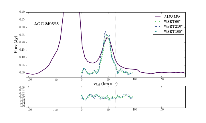
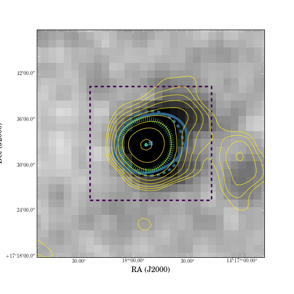
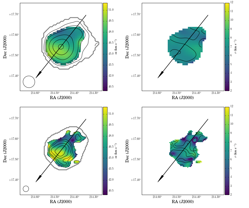
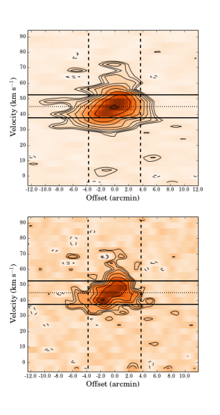
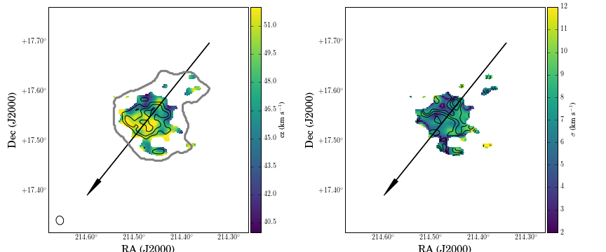
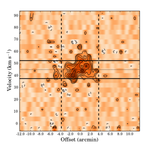
Figure 17: ALFALFA and WSRT data for AGC 249525 as in Figure 8 but with H i column density contours at [4, 6, 8, 15, 25, 35] $\times 10^{18}$, [0.9, 1.5, 2, 3, 4, 5] $\times 10^{19}$, and [3, 4, 5] $\times 10^{19}$ atoms cm^-2 for the 210^′′,105^′′, and 60^′′ data and velocity contours at [46, 48, 50] km s^-1.

AGC 249565: This source was chosen for its high $\bar{N}_{HI}$. Figure 17 shows the H i data for AGC 249565. At the ALFALFA resolution, its H i morphology is exceptionally smooth and it shows evidence for ordered motion in its velocity field (although it is barely resolved). At the higher 105^′′ angular resolution, it shows some elongation, especially in the outer H i contours, but the core of the source remains smooth and undisturbed, and the velocity gradient is still present in the velocity field and position-velocity slice, although the position-velocity slice also shows some clumpy structure. Since this source was robustly detected in the 105^′′ WSRT data, it was also imaged with a 60^′′ taper. At this resolution its H i morphology starts to become clumpy, but this may be a S/N limitation rather than a true change in morphology. In the position velocity slices in Figures 5 and 17, a velocity extent of 10 km s^-1 is indicated by the solid lines (around a center of 24 km s^-1), with a spatial extent of 5.6^′ indicated by the vertical dashed line. The velocity extent is most clearly seen in the 210^′′ data, although it is still present in the outer envelope at higher resolution. The implication of this is discussed in Section 4.3. The WSRT spectrum matches the ALFALFA spectrum well.

AGC 249393: This object was selected for its isolation within the ALFALFA survey data. It is the largest and lowest $\bar{N}_{HI}$ source observed with WSRT. Unfortunately, it is also the only source for which the final imaging was done with only a single track. (The second track had a substantial number of antennas missing and so could not be effectively tapered.) The source is an apparent non-detection, but is consistent with being at the noise level. In Figure 19 the ALFALFA spectrum is shown with spectra extracted from the WSRT dirty cubes with an aperture of radius 5^′, consistent with the ALFALFA H i size. The noise in the WSRT spectra are consistent with the non-detection. In addition, confidence contours from a moment zero map of the dirty data cube (velocity range indicated in the spectra figure) are shown, and there is evidence at the 2-$\sigma$ level that the source is present. However, we were unable to isolate the source for cleaning and do not report any H i parameters from the WSRT data except for an approximate peak column density value based on the moment zero map from the dirty data. The peak column density seen in the 210^′′ map is consistent with the ALFALFA $\bar{N}_{HI}$ value.

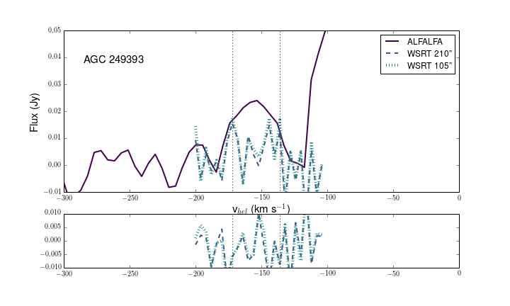
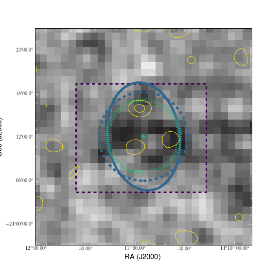
Figure 19: ALFALFA and WSRT data for AGC 249393 as in the top row of Figure 8. AGC 249393 is a non-detection in the WSRT data and an aperture of radius 5^′ (shown by the dotted green circle) is used for extracting the spectra.