Soft Black Hole Absorption Rates as Conservation Laws

Abstract

The absorption rate of low-energy, or soft, electromagnetic radiation by spherically symmetric black holes in arbitrary dimensions is shown to be fixed by conservation of energy and large gauge transformations. We interpret this result as the explicit realization of the Hawking-Perry-Strominger Ward identity for large gauge transformations in the background of a non-evaporating black hole. Along the way we rederive and extend previous analytic results regarding the absorption rate for the minimal scalar and the photon.

Soft Black Hole Absorption Rates as Conservation Laws

^aBrown University
Department of Physics
182 Hope St, Providence, RI 02912
^aMichigan State University
Department of Physics and Astronomy
East Lansing, MI 48824

^bHarvard University
Center for Mathematical Science and Applications
1 Oxford St, Cambridge, MA 02138

savery@msu.edu, schwab@cmsa.fas.harvard.edu

 

1 Introduction

Recently, a number of intriguing connections have been made between three physical ideas: “large gauge transformations”, “memory” effects [1, 2, 3], and soft theorems (e.g., in [4]). Beyond showing old results [5, 6, 7, 8] are the result of underlying symmetry principles, these results have motivated new investigations into soft scattering and memory [9]. This paper extends this “triangle” of related phenomena into a “square”; the new vertex being low energy absorption rates.

The basic insight is that local transformations that have nonvanishing support on the boundary of spacetime need not be gauged, in which case they are physically relevant symmetries with all that entails: conserved currents, charges, and Ward identities. The transformations are energy-preserving shift symmetries: inhomogeneous transformations of the field. Shift symmetries suggest spontaneous symmetry breaking, and indeed one can interpret the transformations that are not isometries of the vacuum as spontaneously broken symmetry generators. With new conserved charges in theories of gravity, it is natural to ask, as Hawking–Perry–Strominger (HPS) did [11], about the implications for black hole evaporation.

While the exact role of these large gauge charges in the black hole information problem has not been fully understood as of yet, we show that shift symmetries of the above kind constrain the form of low energy black hole absorption. Indeed, we show that conservation of energy along with large gauge symmetry conservation laws fix the leading low-energy photon absorption rate of spherically symmetric black holes in $(p+2)$-dimensions. Beyond the conceptual advance in clarifying the role of large gauge transformations for black hole physics, and in demonstrating that low energy absorption follows from symmetry arguments, our result for absorption of angular momentum $\ell$ electromagnetic waves for general $p$ and general charge $Q$ black holes in asymptotically flat space appears to be a new result in the literature. Insofar as Weinberg’s soft theorem is equivalent to the Ward identity for large gauge transformations, one might state our basic result as “Weinberg’s soft theorem fixes the leading low energy black hole absorption rate”; however, we prefer to say that (large) gauge symmetry implies both Weinberg’s soft theorem and low energy black hole absorption.

This paper serves as an illustration of the basic idea. The approach can obviously be straightforwardly generalized in a number of directions. The liminal arguments presented here apply to any other fields with inhomogeneous symmetry transformations—shift symmetries—including gravitons and gravitinos, cf. [17, 18]. One should be able to generalize our results to spinning black holes and black branes, as well. Minor modifications should allow one to apply our methods to asymptotically anti-de Sitter spacetimes, which should give low energy transport coefficients. Let us further note that the conservation laws we write down are valid quite generally, even in spacetimes without an event horizon.

We present the calculation as a classical scattering problem. This serves two purposes: first, it agrees better with the existing black hole scattering literature and second, it may make the calculation accessible to a broader audience. The latter is particularly important, given confusion observed by the authors regarding the significance of HPS [19, 20] and more generally the connection between large gauge transformations and infrared physics [21, 22].

Our paper is organized as follows. In the next section, we present the conventions we be use in the rest of the paper. In sec. 3, we derive the general result for minimal scalar found in [23] using only conservation of energy and the shift symmetry of the scalar. We show that these two symmetries fix the absorption of low-energy scalar waves uniquely. The constant shift symmetry of the minimal scalar serves as a toy version of the electromagnetic gauge symmetry. Many of the equations and much of the reasoning carry over to the electromagnetic case with only small changes. We then expand this analysis to the photon in sec. 4. Finally, we conclude with a discussion of the results and an outlook describing future work. In the appendices, we collect some useful results for reference.

2 Conventions

Following Das–Gibbons–Mathur (DGM) [23], we work with $(p+2)$-dimensional spherically symmetric black hole spacetime metrics of the form

$$ds^{2}=-f(r)dt^{2}+g(r)\big{(}dr^{2}+r^{2}d\Omega_{p}^{2}\big{)},$$ (1)

with horizon at radius $r=r_{H}$ which is determined by $f(r_{H})=0$. The squared line element on the unit $p$-sphere is denoted by $d\Omega_{p}^{2}$. The area of the horizon is given by

$$A_{H}=\big{(}r_{H}^{2}g(r_{H})\big{)}^{\frac{p}{2}}\omega_{p}=R_{H}^{p}\omega_{p}\qquad\omega_{p}=\frac{2\pi^{\frac{p+1}{2}}}{\Gamma(\frac{p+1}{2})},$$ (2)

where $\omega_{p}$ is the volume of the unit $p$-sphere and $R_{H}$ is the normalized radius of the sphere, defined from the above by $R_{H}^{2}=r_{H}^{2}g(r_{H})$. The functions $f(r)$ and $g(r)$ are given for the Schwarzschild black hole and Reissner–Nordström (RN) black holes in Appendix A. The functions $g(r)$ and $f(r)$ have particularly nice properties for our calculation. The former is finite at the horizon of the black hole while the latter is of order ${\cal O}(r-r_{H})^{2}$ at the horizon. Note these coordinates are valid outside the horizon, at $r>r_{H}$. For the extremal RN black hole, the horizon gets mapped to $r_{H}=0$ and the function $g(r)$ diverges at the horizon in this case. The exact expressions for $p+2$ dimensions and more details can be found in appx A.

3 Minimal Scalar

The minimal scalar enjoys a shift symmetry $\phi\to\phi+\epsilon$ that one can think of as a toy version of the large gauge transformations to be considered in the sequel. While the low energy $\ell=0$ absorption result we calculate already exists in [23], the connection to this symmetry has not been emphasized.

Begin by considering a massless, minimally coupled scalar $\phi$ in an arbitrary curved background:

$$S=\int\mathrm{d}^{p+2}x\sqrt{-g}\,\tfrac{1}{2}g^{\mu\nu}\partial_{\mu}\phi\partial_{\nu}\phi.$$ (3)

For the metric in (1), the equations of motion take the form

$$E(\phi)=-\frac{1}{f(r)}\partial_{t}^{2}\phi+\frac{1}{r^{p}\sqrt{f\,g^{p+1}}}\partial_{r}\left(r^{p}\sqrt{f\,g^{p-1}}\partial_{r}\phi\right)+\frac{1}{g(r)r^{2}}\hat{\Delta}_{p}\phi,$$ (4)

where $\hat{\Delta}_{p}$ is the Laplacian on the unit $p$-sphere. Let us use the time translation and spherical symmetry of the background to decompose $\phi(x)$ into modes:

$$\phi(t,r,\Omega)=\sum_{\ell,m}\int\frac{\mathrm{d}\omega}{2\pi}\phi_{\omega,\ell,m}(r)\,Y_{\ell,m}(\Omega)e^{-i\omega t}.$$ (5)

In the following, we will perform our analysis on a $\ell=0$ fixed $\omega$ mode, frequently suppressing the mode labels to avoid notational clutter.

3.1 Symmetries

We will use two symmetry properties of the scalar field. First of all, the rigid shift symmetry with transformation

$$\phi(x)\mapsto\phi(x)+\epsilon,$$ (6)

where $\partial_{\mu}\epsilon=0$. The corresponding conserved current is given by

$$j^{\mu}=\epsilon g^{\mu\nu}\partial_{\nu}\phi,$$ (7)

which almost trivially satisfies

$$\nabla_{\mu}j^{\mu}=E(\phi)\delta_{\epsilon}\phi,$$ (8)

as required. This is the statement of conservation of canonical momentum in [24, 25]. Additionally, we will need conservation of energy. For this we need the stress tensor, which is given by

$$T^{\mu\nu}=\frac{2}{\sqrt{-g}}\frac{\delta S}{\delta g_{\mu\nu}}=\nabla^{\mu}\phi\nabla^{\nu}\phi-\frac{1}{2}g^{\mu\nu}g^{\rho\sigma}\nabla_{\rho}\phi\nabla_{\sigma}\phi$$ (9)

It is possible to express $T$ in terms of $j$, but the conservation law is independent of the conservation of $j$. As our metric has a timelike Killing vector, $\xi=\partial_{t}$, conservation of energy follows

$$\nabla_{\mu}T^{\mu 0}=\nabla_{\mu}(T^{\mu\nu}\xi_{\nu})=0.$$ (10)

3.2 Solutions

In order to find the $\ell=0$ low energy absorption rate, we need to solve the $\ell=0$ equation of motion in two limits: the asymptotically flat region, $r\gg r_{H}$, where $f,g\to 1$; and the near-horizon region, $(r-r_{H})\ll R_{H}$. The conservation laws relate the two regions’ small $\omega$ behavior without having to say anything about the interior. Note that solving in these two regions is necessary, anyway, to define what we mean by the absorption rate, and to impose physically appropriate boundary conditions at the horizon.

Asymptotically Flat Limit

For $r\gg r_{H}$, $f(r)=g(r)=1$ and we just have the flat equations of motion. For $\ell=0$, the solution is

$$\phi_{\text{flat}}(r)=(\omega r)^{-\frac{p-1}{2}}\left(A_{\omega}\,J_{\frac{p-1}{2}}(\omega r)+B_{\omega}\,Y_{\frac{p-1}{2}}(\omega r)\right)\qquad r\gg r_{H},$$ (11)

for $p>1$. We take two further limits of the above result. First, taking $\omega r\gg 1$, we may use the Bessel functions’ large argument asymptotic form to write

$$\phi_{\text{flat}}(r)\simeq\frac{2}{\sqrt{2\pi(\omega r)^{p}}}\left(A_{\omega}\cos\big{(}\omega r-\tfrac{(p-2)\pi}{4}\big{)}+B_{\omega}\sin\big{(}\omega r-\tfrac{(p-2)\pi}{4}\big{)}\right)\qquad\omega r\gg 1.$$ (12)

Second, taking $\omega r\ll 1$ (but keeping $r\gg r_{H}$) we may use the small argument limit of the Bessel functions to write

$$\phi_{\text{flat}}\simeq\frac{1}{2^{\frac{p-1}{2}}}\left(\frac{A_{\omega}}{\Gamma(\frac{p+1}{2})}-\frac{B_{\omega}\Gamma(\frac{p-1}{2})}{\pi}\left(\frac{\omega r}{2}\right)^{-(p-1)}\right)\qquad\omega r\ll 1.$$ (13)

It is the above limiting form which gets related to the near-horizon physics by the two conservation laws.

Near-Horizon Limit

For the near-horizon analysis, it is convenient to define a new radial coordinate $\rho$ ($\tau$ in [23]) such that

$$\partial_{\rho}=r^{p}\sqrt{f(r)\,g(r)^{p-1}}\partial_{r}.$$ (14)

With this radial coordinate, the equation of motion takes the form

$$E(\phi)=\frac{1}{f(r)\big{(}r^{2}g(r)\big{)}^{p}}\left[\partial_{\rho}^{2}-\big{(}r^{2}g(r)\big{)}^{p}\partial_{t}^{2}+f(r)\big{(}r^{2}g(r)\big{)}^{p-1}\Delta_{p}\right]\phi.$$ (15)

At the horizon of a nonextremal black hole, $f$ has a double zero and $g$ is regular. The $\ell=0$ mode equation for $r\sim r_{H}$ becomes

$$\big{(}\partial_{\rho}^{2}+R_{H}^{2p}\omega^{2}\big{)}\phi_{\omega}(\rho)=0,$$ (16)

with solutions $\exp(\pm i\omega R_{H}^{p}\rho)$. Ingoing boundary conditions choose the negative sign. Thus, for small $r$ the solution takes the form

$$\phi_{\omega}(r)\simeq\phi_{H}\,e^{-i\omega R_{H}^{p}\rho}.$$ (17)

Absorption Rate

We can use the asymptotically flat solutions to give the absorption rate in terms of $A_{\omega}$ and $B_{\omega}$. Explicitly, from eq. (12) the absorption rate is given by

$$\Gamma_{\text{abs}}=1-\left|\frac{1-i\frac{B_{\omega}}{A_{\omega}}}{1+i\frac{B_{\omega}}{A_{\omega}}}\right|^{2}.$$ (18)

Instead of working with the coefficients $A$ and $B$, let us rewrite the ratio $B/A$ in terms of $\phi^{\prime}(R)/\phi(R)$ for $R\gg r_{H}$ and $\omega R\ll 1$. Using (13), we may write

$$\frac{B_{\omega}}{A_{\omega}}=\left(\frac{\omega R}{2}\right)^{p-1}\frac{\pi(p-1)}{2\,\Gamma(\frac{p+1}{2})^{2}}\frac{R\frac{\phi^{\prime}(R)}{\phi(R)}}{p-1+R\frac{\phi^{\prime}(R)}{\phi(R)}},$$ (19)

after dropping subleading terms in $\omega R$. Below we show that conservation of energy and “canonical momentum” fixes $\phi^{\prime}(R)/\phi(R)$, for $R\gg r_{H}$ and $\omega R\ll 1$, in terms of $\phi^{\prime}(r_{H})/\phi(r_{H})$. From the near-horizon solution, we see that

$$\frac{\phi^{\prime}(r_{H})}{\phi(r_{H})}=-i\omega\sqrt{\frac{g(r_{H})}{f(r_{H})}},$$ (20)

where there is an implicit regulator on $r_{H}$, since $f(r)$ has a double zero at the horizon. We will see that the regulator cancels out of the absorption rate.

3.3 Conservation laws

We have two conserved currents, eqs. (7) and (10), corresponding to shift symmetry and time translation symmetry. The shift symmetry implies the existence of a constant mode, which we would like to relate to the $\omega\to 0$ limit of the $\ell=0$ ($s$-wave) mode. The conservation laws imply that for any subregion $R$,

$$\oint_{\partial R}\star j=\int_{R}d\star j=\int_{R}\bm{\epsilon}E(\phi)\delta\phi\overset{w}{=}0,$$ (21)

where we use the notation of [26] to emphasize that the last equality follows only after using equations of motion. It is up to us to find a convenient contour $C=\partial R$ that usefully constrains the dynamics under consideration. To follow HPS, it would seem natural to choose the spacetime outside the black hole event horizon; however, we need to regulate the contour. For the steady state absorption process under consideration, the following regulated contour seems most convenient:

$$C=\Sigma_{-}\cup\Lambda\cup\Sigma_{+}\cup H,$$ (22)

with

$$\begin{aligned} \Lambda&:r=R\quad t\in[-T,T]\\ \Sigma_{-}&:t=-T\quad r\in[r_{H}+\delta,R]\\ \Sigma_{+}&:t=T\quad r\in[r_{H}+\delta,R]\\ H&:r=r_{H}+\delta\quad t\in[-T,T].\end{aligned}.$$ (23)

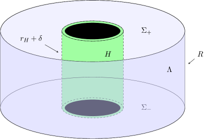
Figure 1: A cartoon of the integration regions. Time runs upward and each $S^{1}$ of the cylinder represents an $S^{p}$. The top and bottom of the cylinder are at $\pm T$, the respective regions $\Sigma_{\pm}$ are the spatial integration regions. $\Lambda$ is blue, $H$ is green. At a distance of $\delta\ll R_{H}$ to the horizon of the black hole, located at $r=r_{H}$, we put a stretched horizon. Similarly, at $R\gg r_{H}$ we put a stretched infinity. At the end of the calculation we will remove both regulators at the same time.

See Fig. 1 for a depiction of the surfaces. Note that we are not working with null surfaces, which is different from HPS; although this should not change the physics. In the limit $\delta\to 0$ and $R,T\to\infty$ we should cover the exterior spacetime. More specifically we shall take $\delta\to 0$ first, and $T$ and $R$ large with $T\gg R$.

Using the shift current and the contour $C$, (21) becomes

$$\int_{r_{H}}^{R}\mathrm{d}r\,r^{p}\sqrt{\frac{g(r)^{p+1}}{f(r)}}\int_{0}^{\infty}\mathrm{d}\omega\frac{\sin(\omega T)}{\pi\omega}\omega^{2}(\phi_{\omega}(r)-\phi_{-\omega}(r))\\ =R^{p}\sqrt{f(R)g(R)^{p-1}}\int_{-\infty}^{\infty}\mathrm{d}\omega\frac{\sin(\omega T)}{\pi\omega}\phi^{\prime}_{\omega}(R)-r_{H}^{p}\sqrt{f(r_{H})g(r_{H})^{p-1}}\int_{-\infty}^{\infty}\mathrm{d}\omega\frac{\sin(\omega T)}{\pi\omega}\phi^{\prime}_{\omega}(r_{H}).$$ (24)

Recalling that

$$\lim_{T\to\infty}\frac{\sin(\omega T)}{\pi\omega}=\delta(\omega),$$ (25)

we find in the small $\omega$ limit the spacelike portions of the contour are subleading and thus

$$R^{p}\sqrt{f(R)g(R)^{p-1}}\phi^{\prime}_{\omega}(R)\simeq r_{H}^{p}\sqrt{f(r_{H})g(r_{H})^{p-1}}\phi^{\prime}_{\omega}(r_{H})+O(\omega^{2}).$$ (26)

As we noted before, this result can be found in [24, 25] as conservation of canonical momentum. Notice that the conservation law is a useful constraint, precisely because it is indifferent to the behavior of $\phi$ (or equivalently the metric coefficients $f$ and $g$) in the middle region away from the horizon and asymptotically flat region.

The shift conservation law (26) is not sufficient to determine the absorption rate. We need two conditions relating the near-horizon mode behavior to the asymptotic mode behavior. Thus, let us turn to conservation of energy.

Let us take the same contours as in (23). Note that there is an important difference from the shift symmetry: all of the spherical modes contribute to the energy. Let us work on the spacelike slices first:

$$\int_{\Sigma}\star J=-\frac{1}{2}\int\mathrm{d}\Omega\,r^{p}\sqrt{f(r)g(r)^{p-1}}\phi\phi^{\prime}\Big{|}_{r_{H}}^{R}-\frac{1}{2}\int\mathrm{d}\Omega\int\mathrm{d}r\,r^{p}\sqrt{fg^{p+1}}\left[\frac{\dot{\phi}^{2}}{f}-\frac{\phi\ddot{\phi}}{f}-\phi\,E(\phi)\right].$$ (27)

Note that the second term is $O(\omega)$, after using the equations of motion. The spacelike integrals again give subleading corrections to the leading result when one takes $T\to\infty$. The timelike integrals give

$$\int_{\Lambda+H}\star J=\omega_{p}\int\frac{\mathrm{d}\omega_{1}}{2\pi}\int\mathrm{d}\omega_{2}\,\frac{\sin((\omega_{1}+\omega_{2})T)}{\pi(\omega_{1}+\omega_{2})}(-i\omega_{2})\,\left[r^{p}\sqrt{f(r)g(r)^{p-1}}\phi^{\prime}_{\omega_{1}}(r)\phi_{\omega_{2}}(r)\right]_{r_{H}}^{R}.$$ (28)

In the large $T$ limit, the $\sin$ factor gives a $\delta(\omega_{1}+\omega_{2})$, and we are left with

$$R^{p}\sqrt{f(R)g(R)^{p-1}}\phi_{-\omega}(R)\phi_{\omega}^{\prime}(R)=r_{H}^{p}\sqrt{f(r_{H})g(r_{H})^{p-1}}\phi_{-\omega}(r_{H})\phi_{\omega}^{\prime}(r_{H}).$$ (29)

Combining conservation of energy with the shift conservation law we find that $\phi_{\omega}$ approaches the constant shift mode in the small $\omega$ limit:

$$\phi_{\omega}(r_{H})\simeq\phi_{\omega}(R)+O(\omega),$$ (30)

and one can find the identity

$$R^{p}\sqrt{f(R)g(R)^{p-1}}\frac{\phi^{\prime}(R)}{\phi(R)}=r_{H}^{p}\sqrt{f(r_{H})g(r_{H})^{p-1}}\frac{\phi^{\prime}(r_{H})}{\phi(r_{H})}.$$ (31)

Using that $f(R),g(R)\to 1$ for large $R$ and (20), this becomes

$$R\frac{\phi^{\prime}(R)}{\phi(R)}=-i\omega R\,\left(\frac{R_{H}}{R}\right)^{p},$$ (32)

which we can plug into (19) and (18) to find the absorption rate. In the limits we are working, one finds

$$\Gamma_{\text{abs}}=4\frac{\pi}{\Gamma(\frac{p+1}{2})^{2}}\left(\frac{\omega R_{H}}{2}\right)^{p},$$ (33)

which agrees with Ref. [23], after using standard Gamma function identities. Note that the dependence on all of the regulators has dropped out. Additionally, the metric dependence has also dropped out. This is a well-known result: The absorption rate for minimal scalars only depends on the area $A_{H}$ of the black hole horizon, but is otherwise independent of the function $g(r)$. We will see that this is not true for electromagnetic radiation.

4 Photon

We now turn to the photon. In the last section, we used the shift symmetry of the massless scalar to derive our results. In the present case, the shift symmetry is replaced by the so called (large) gauge symmetry. That is, transformations of the photon field $A_{\mu}$

$$A_{\mu}\to A_{\mu}+\partial_{\mu}\lambda(x),$$ (34)

where $\lambda(x)$ is a function of the coordinates on the sphere $\theta^{A}$ at asymptotic infinity, i.e.,

$$\lim_{r\to\infty}\lambda(t,r,\theta^{A})=\lambda(\theta^{A}).$$ (35)

These are the so called large gauge transformations defined in [27, 6, 5]. To fix our conventions, on a curved background with metric $g_{\mu\nu}(x)$, we take the Lagrangian density for the photon to be

$$\mathscr{L}=-\frac{\sqrt{-g}}{4}F_{\mu\nu}F^{\mu\nu},$$ (36)

which implies the equations of motion

$$E^{\nu}=-\nabla_{\mu}F^{\mu\nu}=-\Box A_{\nu}+\nabla_{\nu}(\nabla^{\mu}A_{\mu})+{R^{\lambda}}_{\nu}A_{\lambda}.$$ (37)

The Noether current for gauge transformations—the derivation can be found in, e.g., [26]—is given by

$$j^{\mu}=F^{\mu\nu}\partial_{\nu}\lambda.$$ (38)

Note that the Noether current has similarities with the shift current (7); it depends on the field strength $F_{\mu\nu}$ and is accompanied by the transformation parameter $\lambda(x)$. To draw a parallel with the minimal scalar let us note that the time component of $j^{\mu}$—which we ultimately use to determine a conserved quantity for this current—only depends on the canonical momentum density $F_{0i}=E_{i}$ of the field $A_{i}$. We may again speak about the conservation of canonical momentum. However, there are also glaring dissimilarities. The new ingredient here is that $\lambda$ is a function on the sphere with a clearly determined boundary value at $r\to\infty$. Apart from that, $\lambda$ does not, a priori, satisfy any constraints, so in the bulk of the space time, $\lambda(x)$ is undetermined. The current is conserved for all $\lambda$, so that it is up to us to determine the gauge transformations that give useful conservation laws. We will find appropriate constraints for it in due course. In particular, we will show that the conservation law is useful when $\lambda$ solves the $\omega=0$ photon equation with appropriate fall off for large $r$. It is clear however, that, since $\lambda$ is now a function of at least the coordinates on the sphere, we should be able to get more than just a single $\ell$ mode of the field $A_{\mu}$. Indeed, we see that conservation of canonical momentum for the minimal scalar becomes conservation of canonical momentum density for the photon; there is now a zero mode for every $\ell>0$. The on-shell conservation of $j^{\mu}$ follows directly

$$\nabla_{\mu}j^{\mu}=-E^{\nu}\nabla_{\nu}\lambda+\frac{1}{2}F^{\mu\nu}[\nabla_{\mu},\nabla_{\nu}]\lambda=-E^{\nu}\nabla_{\nu}\lambda.$$ (39)

As with the minimal scalar, we also need to give the stress tensor for the photon field in curved spacetime. It takes the form

$$T_{\mu\nu}=F_{\mu\rho}{F^{\rho}}_{\nu}+\frac{1}{4}g_{\mu\nu}F_{\rho\sigma}F^{\rho\sigma}.$$ (40)

Its conservation follows from

$$\nabla^{\mu}T_{\mu\nu}=\frac{1}{2}E^{\rho}F_{\rho\nu}-\frac{1}{2}F^{\rho\sigma}({R^{\lambda}}_{\nu\rho\sigma}+{R^{\lambda}}_{\sigma\nu\rho}+{R^{\lambda}}_{\rho\sigma\nu})A_{\lambda},$$ (41)

where the second term vanishes due to the first Bianchi identity for the Riemann tensor.

To proceed, we shall write down a mode expansion for $A_{\mu}$. As the background (1) is spherically symmetric, we would like to exploit this circumstance by labeling modes with the following commuting set of operators: since the spacetime is static and spherically symmetric, we have a timelike Killing vector $\partial_{t}$ and rotational symmetry $SO(p+1)$. Thus we can use the Hamiltonian $H=i\mathcal{L}_{\partial_{t}}$ and the $SO(p+1)$ Casimir $J^{2}$. In four dimensions ($p=2$), we also include the parity transformation $P$. The parity is relevant in this special case, as it allows us to distinguish the spherical harmonics $\hat{\nabla}Y_{lm}$ from $\hat{W}_{A}=\hat{\epsilon}_{AB}\hat{\nabla}^{B}Y_{lm}$. In higher dimensions, the analogous two modes have different $J^{2}$. For convenience, let us decompose the Lorentz vector index $\mu$ into $i,j,k\in(t,r)$ and $A,B,C\in\Omega$. The $SO(p+1)$ Casimir acts as

$$J^{2}A_{j}=-\hat{\Delta}A_{j}\qquad J^{2}A_{A}=-(\hat{\Delta}-p+1)A_{A}.$$ (42)

If we let $m$ represent the set of eigenvalue(s) of the generators of the Cartan subalgebra of $SO(p+1)$ we may symbolically write even higher dimensional spherical harmonics as $Y_{\ell m}$. Notice that $m$ is a single number only for $p=2$. As we will only use a very limited set of properties of the spherical harmonics on $S^{p}$, we will not give many details about these functions. More details can be found in [28, 29]. For us, the relevant information is the following. On each $S^{p}$, there are two kinds of vector spherical harmonics: there is a gradient mode, $\hat{\nabla}_{A}Y$, and there is a divergence-free mode, $\hat{W}_{A}$, with $\hat{\nabla}^{A}\hat{W}_{A}=0$ [28, 29]. These modes have eigenvalues

$$\hat{\Delta}(\hat{\nabla}_{A}Y_{\ell})=-\big{[}\ell(\ell+p-1)-(p-1)\big{]}(\hat{\nabla}_{A}Y_{\ell})\qquad\hat{\Delta}\,\hat{W}^{(\ell)}_{A}=-\big{[}\ell(\ell+p-1)-1\big{]}\hat{W}^{(\ell)}_{A},$$ (43)

and thus

$$J^{2}(\hat{\nabla}_{A}Y_{\ell})=\ell(\ell+p-1)\hat{\nabla}_{A}Y_{\ell}\qquad J^{2}\hat{W}^{(\ell)}_{A}=[\ell(\ell+p-1)+p-2]\hat{W}^{(\ell)}_{A}.$$ (44)

Note that it is only for $p=2$ that the two Casimir eigenvalues coincide. The degeneracies of the gradient and divergence-free mode are given by

$$d_{s}(p,\ell)=\frac{(\ell+p-2)!}{(p-1)!\,\ell!}(2\ell+p-1)\qquad d_{V}(p,\ell)=\frac{\ell(\ell+p-1)\,(2\ell+p-1)(\ell+p-3)!}{(p-2)!\,(\ell-1)!},$$ (45)

respectively. From (44) it is quite obvious that the $\hat{W}$ cannot mix with the scalar modes since they have a different value for the Casimir for $p>2$. For the special case of $p=2$ we use—as we explained above—parity to distinguish these two modes.

To proceed, we define a “gradient mode”

$$A^{(+)}_{\mu}=\big{(}A(r)Y_{\ell,m}(\Omega),B(r)Y_{\ell,m}(\Omega),C(r)\hat{\nabla}_{A}Y_{\ell,m}\big{)}e^{-i\omega t},$$ (46)

as well as a “solenoidal mode” which is given by

$$A^{(-)}_{\mu}=\big{(}0,0,D(r)\hat{W}^{(\ell)}_{A}(\Omega)\big{)}e^{-i\omega t}.$$ (47)

For convenience, throughout the rest of the text, we may refer to these as $+$ and $-$ modes, respectively. In the following, we focus on the gradient or $+$ mode and give only a few comments on the solenoidal mode.

Let us also define a “longitudinal” or gauge mode:

$$L_{\mu}=\partial_{\mu}(\Lambda(r)Y_{lm}(\Omega)e^{-i\omega t})=\big{(}-i\omega\Lambda(r)Y_{lm}(\Omega),\Lambda^{\prime}(r)Y_{lm}(\Omega),\Lambda(r)\hat{\nabla}_{A}Y_{lm}(\Omega)\big{)}e^{-i\omega t}.$$ (48)

For $\omega>0$ this mode decouples and is unphysical, as expected; however, in the $\omega\to 0$ limit the longitudinal and gradient modes degenerate as we see below explicitly in temporal gauge.

4.1 Gauge choice and radial equations of motion

So far, we haven’t chosen a gauge. We shall remedy this situation presently. It turns out that the calculation is particularly convenient in temporal gauge

$$A_{t}=0.$$ (49)

When imposing this gauge on the $+$ mode defined above we find that $A=0$ and $B$ is related to $C^{\prime}(r)$ via the Gauss constraint, while the $-$ mode already satisfies the gauge condition. The $+$ mode then takes the form

$$A^{+}_{\mu}=\left(0,C^{\prime}(r)\frac{\ell(\ell+p-1)f(r)}{\ell(\ell+p-1)f(r)-\omega^{2}r^{2}g(r)}Y_{lm},C(r)\hat{\nabla}_{A}Y_{lm}\right)_{\mu}e^{-i\omega t}.$$ (50)

The rest of the equations of motion imply that this mode is a solution provided $C(r)$ satisfies the radial equation of motion

$$C^{\prime\prime}(r)+\frac{\mathrm{d}}{\mathrm{d}r}\log\left[\frac{r^{p}\sqrt{f(r)g(r)^{p-1}}}{\ell(\ell+p-1)f(r)-\omega^{2}r^{2}g(r)}\right]C^{\prime}(r)+\left(\omega^{2}\frac{g(r)}{f(r)}-\frac{\ell(\ell+p-1)}{r^{2}}\right)C(r)=0.$$ (51)

We may also calculate the field strength $F_{\mu\nu}$, which we use extensively in the calculation below. It is given by

$$\begin{aligned} F_{tr}&=i\omega\frac{\ell(\ell+p-1)f(r)}{\omega^{2}r^{2}g(r)-\ell(\ell+p-1)f(r)}C^{\prime}(r)\,Y_{\ell m}e^{-i\omega t}\\ F_{tA}&=-i\omega C(r)\,(\hat{\nabla}_{A}Y_{\ell m})e^{-i\omega t}\\ F_{rA}&=\frac{\omega^{2}r^{2}g(r)}{\omega^{2}r^{2}g(r)-\ell(\ell+p-1)f(r)}C^{\prime}(r)\,(\hat{\nabla}_{A}Y_{\ell m})e^{-i\omega t}\\ F_{AB}&=0\end{aligned}.$$ (52)

We put emphasis on this mode over the solenoidal mode as it is the one which degenerates with the pure gauge mode $\lambda(x)$. Information regarding the solenoidal mode can be found in appx B. Observe that both the gradient and solenoidal mode start with $\ell=1$, not $\ell=0$, since the photon has spin one.

As for $\lambda(x)$, after imposing the gauge condition, we find that the residual gauge freedom is given by $\lambda=\Lambda_{\ell m}(r)Y_{\ell m}(\Omega)$. This corresponds to a “longitudinal photon” of the form

$$L_{\mu}=\partial_{\mu}\lambda=(0,\,\Lambda_{\ell m}^{\prime}(r)Y_{\ell m}(\Omega),\,\Lambda_{\ell m}(r)\hat{\nabla}_{A}Y_{\ell m}(\Omega)).$$ (53)

Note that this is indeed the $\omega\to 0$ limit of $A^{(+)}_{\mu}$, which suggests an identification $C_{\omega}\to\Lambda$ as $\omega\to 0$. $C_{\omega}(r)$ solves a second order differential so there are only two physically realized profiles of $r$ as $\omega\to 0$. With this observation, one may correctly anticipate that the interesting choice of $\Lambda_{\ell m}(r)$ should be one of those modes.

4.2 Solutions for the gradient mode

We are now in a position to study the solutions of eq. (51). It turns out that it is sufficient to study the equation in three limits. This is an important difference from the $\ell=0$ minimal scalar calculation, where we only needed two limits. We first study the case $r\gg r_{H}$ where the functions $f(r)$ and $g(r)$ in eq. (1) go to $1$. Thus (51) turns into the radial equation of motion for a photon propagating in flat space. The second limit is the near horizon limit $r-r_{H}=\delta\ll R_{H}$. Finally, we investigate the equation (51) on the whole space in the $\omega\to 0$ limit.

Asymptotically Flat Limit

Let us first turn to the asymptotically flat case. We find that the equation of motion for the function $C(r)$ becomes the second order ordinary differential equation

$$C^{\prime\prime}(r)+\frac{(p-2)\omega^{2}r^{2}-p\,\ell(\ell+p-1)}{\omega^{2}r^{3}-\ell(\ell+p-1)r}C^{\prime}(r)+\left(\omega^{2}-\frac{\ell(\ell+p-1)}{r^{2}}\right)C(r)=0$$ (54)

which has a general solution in terms of combinations of Bessel functions of the first kind $J_{\alpha}(r)$, and second kind $Y_{\alpha}(r)$. Explicitly, one finds the solution

$$C_{\rm flat}(r)=C_{1}\frac{\ell\,J_{\ell+\frac{p-1}{2}}(\omega r)-\omega r\,J_{\ell+\frac{p-3}{2}}(\omega r)}{(\omega r)^{\frac{p-1}{2}}}+C_{2}\frac{\ell\,Y_{\ell+\frac{p-1}{2}}(\omega r)-\omega r\,Y_{\ell+\frac{p-3}{2}}(\omega r)}{(\omega r)^{\frac{p-1}{2}}}.$$ (55)

for all $p>1$ and all $\ell>0$.

Just as for the scalar, two further limits are of interest. For $\omega r\gg 1$, the solution takes the form

$$C_{\rm flat}(r)\simeq-\frac{1}{(\omega r)^{\frac{p-2}{2}}}\left[C_{1}\sqrt{\frac{2}{\pi}}\cos\big{(}\omega r-(2\ell+p-2)\tfrac{\pi}{4}\big{)}+C_{2}\sqrt{\frac{2}{\pi}}\sin\big{(}\omega r-(2\ell+p-2)\tfrac{\pi}{4}\big{)}\right].$$ (56)

Conversely, when $\omega r\ll 1$, the solution is asymptotically and to leading order

$$C_{\rm flat}=-C_{1}\frac{\ell+p-1}{2^{\frac{p-1}{2}}\Gamma\left(\ell+\frac{p+1}{2}\right)}\left(\frac{\omega r}{2}\right)^{\ell}-C_{2}\frac{\ell\ \Gamma\left(\ell+\frac{p-1}{2}\right)}{2^{\frac{p-1}{2}}\pi}\left(\frac{\omega r}{2}\right)^{-\ell-p+1}.$$ (57)

We return to (55) in the next section where we examine the conservation laws that lead to the absorption rate. Before we do that though, let us also examine the near-horizon limit of (51).

Near-Horizon Limit

In particular we are interested in the near-horizon limit of (51) for very low frequency. Since the limits do not commute, let us fix a prescription to which we adhere in the rest of the text. In the following, we always take the near-horizon limit before we take the small $\omega$ limit, i.e., $r-r_{H}=\delta\ll\omega r_{H}^{2}$. Then we can rewrite the resulting differential equation in terms of a new radial coordinate $\rho(r)$ such that its derivative

$$\rho^{\prime}(r)=\frac{\ell(\ell+p-1)f(r)-\omega^{2}r^{2}g(r)}{r^{p}\sqrt{f(r)g(r)^{p-1}}},$$ (58)

and the equation of motion becomes

$$C^{\prime\prime}(\rho)+\frac{(r^{2}g(r))^{p-2}}{\omega^{2}-\frac{f(r)}{g(r)}\frac{\ell(\ell+p-1)}{r^{2}}}C(\rho)=0.$$ (59)

At the horizon of a nonextremal black hole, $f(r)$ has a double zero and $g(r)$ is regular. Thus we can make an approximation for $f(r)$ in the near horizon limit where $f(r_{H}+\delta)\approx\frac{1}{2}f^{\prime\prime}(r_{H})\delta^{2}$ and $g(r_{H}+\delta)\approx g(r_{H})$. In the limit defined above, $\delta\ll\omega r_{H}^{2}$ and $\ell$ fixed, the solution to the resulting differential equation is

$$C(\rho)\simeq C_{H}e^{\pm\frac{i\,R_{H}^{p-2}}{\omega}\rho}.$$ (60)

At the horizon of the black hole, we want to choose a solution which is purely ingoing. We can do so by choosing the sign of the exponent appropriately. Note that in the limit we are taking, the derivative of our radial coordinate $\rho^{\prime}(r)<0$, which implies that increasing $r$ is decreasing $\rho$. The ingoing solution is therefore actually the solution with the positive sign in the exponent.

Zero-Energy Limit

We now consider the zero energy limit. In order for the spacelike contributions to drop out of the conservation law, we find that the gauge parameter $\Lambda_{\ell m}(r)$ must satisfy this equation. To derive the solution of the equation of motion for $C(r)$ in the $\omega=0$ limit, we can employ a specific black hole background like Schwarzschild or Reissner–Nordström and then infer the general solution. The equation itself is

$$C^{\prime\prime}(r)+\frac{\partial}{\partial r}\log\left(r^{p}\sqrt{\frac{g(r)^{p-1}}{f(r)}}\right)C^{\prime}(r)-\frac{\ell(\ell+p-1)}{r^{2}}C(r)=0.$$ (61)

The Schwarzschild metric in higher dimensions can be found in appx A.

In the following, we use $r_{H}$ to rewrite the functions $f(r)$ and $g(r)$ in terms of dimensionless variables $x=\frac{r}{r_{H}}$. We insert the functions $f(r)$ and $g(r)$ for the Schwarzschild solution into the $\omega=0$ and get

$$C^{\prime\prime}(x)+\left(\frac{p}{x}-\frac{2(p-1)\left(2x^{p}-x\right)}{x^{2p}-x^{2}}\right)C^{\prime}(x)-\frac{\ell(\ell+p-1)}{x^{2}}C(x)=0.$$ (62)

The solution to this equation is given in terms of hypergeometric ${}_{2}F_{1}$. Specifically, the two independent solutions are

$$C_{\omega=0,p}^{(1)}(r) =\left(\frac{r}{r_{H}}\right)^{\ell-p+1}\frac{1}{\sqrt{g(r)^{p-1}}}{}_{2}F_{1}\left(-\frac{1}{2},\frac{\ell}{p-1};\frac{3}{2}+\frac{\ell}{p-1};\left(\frac{r}{r_{H}}\right)^{2(p-1)}\right)$$ (63)

$$C_{\omega=0,p}^{(2)}(r) =\left(\frac{r}{r_{H}}\right)^{-\ell-2p+2}\frac{1}{\sqrt{g(r)^{p-1}}}{}_{2}F_{1}\left(-\frac{1}{2},-1-\frac{\ell}{p-1};\frac{1}{2}-\frac{\ell}{p-1};\left(\frac{r}{r_{H}}\right)^{2(p-1)}\right)$$ (64)

where we already inserted the form of the general solution where the $g(r)$ parametrizes the dependence of the solution on the specific black hole background.

We need to investigate two limits of these solutions. The near-horizon limit of these functions is easily derived by noticing that the hypergeometric function needs to be evaluated at 1 where it is well known that

$${}_{2}F_{1}(a,b;c;1)=\frac{\Gamma(c)\Gamma(c-a-b)}{\Gamma(c-a)\Gamma(c-b)}$$ (65)

if the real parts $\Re(c)>\Re(a+b)$. This is fulfilled here for the first solution. The function in the second line goes to zero in this limit. Explicitly, the first function becomes

$$C_{\omega=0,p}(r_{H})=\frac{2}{\sqrt{\pi g(r_{H})^{p-1}}}\frac{\Gamma\left(\frac{\ell}{p-1}+\frac{3}{2}\right)}{\Gamma\left(\frac{\ell}{p-1}+2\right)}.$$ (66)

On the other hand, for large r, we want to pick out a solution which goes like $R^{-\ell-p+1}$. For large argument, the hypergeometric function satisfies

$${}_{2}F_{1}(a,b;c;z)=\frac{\pi}{\sin\pi(b-a)}\left(\frac{(-z)^{-a}}{\Gamma(b)\Gamma(c-a)}-\frac{(-z)^{-b}}{\Gamma(a)\Gamma(c-b)}\right)$$ (67)

so the coefficient of the second solution can be adjusted to cancel an unwanted contribution from the first solution. Then

$$C_{\omega=0,p}(R)=\left(\frac{R}{r_{H}}\right)^{-\ell-p+1}.$$ (68)

Later, we will need the ratio of the near-horizon and the flat space value. It is (suppressing some labels on $C$)

$$\frac{C(R)}{C(r_{H})}=\frac{\sqrt{\pi}}{2}g(r_{H})^{-\frac{\ell}{2}}\left(\frac{R_{H}}{R}\right)^{\ell+p-1}\frac{\Gamma\left(\frac{\ell}{p-1}+2\right)}{\Gamma\left(\frac{\ell}{p-1}+\frac{3}{2}\right)}$$ (69)

where we again used the relation $R_{H}^{2}=g(r_{H})r_{H}^{2}$.

Absorption Rate

With the calculations from the first two paragraphs, we can assemble the absorption rate as a function of the ratio of the coefficients $C_{i}$ of the flat space solutions (55). Explicitly, from (56) it follows that the absorption rate is given by

$$\Gamma_{\rm abs}=1-\left|\frac{1-i\frac{C_{2}}{C_{1}}}{1+i\frac{C_{2}}{C_{1}}}\right|^{2}.$$ (70)

Below, in the calculation of the cross section, we will encounter two ratios which we shall give here for later reference. The first is a ratio for the near-horizon solutions

$$\frac{C^{\prime}(r_{H})}{C(r_{H})}=\frac{i\,R_{H}^{p-2}}{\omega}\rho^{\prime}(r)=-i\omega\sqrt{\frac{g(r_{H})}{f(r_{H})}},$$ (71)

where there is an implicit regulator on $r_{H}$, which cancels out of the absorption calculation.

Conversely, when we take the radial coordinate $r$ to be much larger than the radius of the black hole $r\to R\gg r_{H}$, it is appropriate to use (54). Simultaneously taking $\omega R\ll 1$ allows us to use the small argument expansion of the Bessel functions (57). In this limit the following equation is applicable

$$\frac{C_{2}}{C_{1}}=\left(\frac{\omega R}{2}\right)^{2\ell+p-1}\frac{\pi(\ell+p-1)(2\ell+p-1)}{2\ell\,\Gamma(\ell+\frac{p+1}{2})^{2}}\frac{\ell-R\frac{C^{\prime}(R)}{C(R)}}{(\ell+p-1)+R\frac{C^{\prime}(R)}{C(R)}}.$$ (72)

Thus we can turn the absorption rate into a function of the ratio $C^{\prime}(R)/C(R)$ where $R$ is large and try to find an expression for this ratio in terms of other known quantities. This is what we do in the next section.

4.3 Conservation laws

We now show that energy conservation $\nabla_{\mu}T^{\mu 0}=0$ and conservation of the soft current

$$j^{\mu}=F^{\mu\nu}\partial_{\nu}\lambda$$ (73)

is enough to fix the leading low energy absorption rate $\Gamma_{\rm abs}$ for electromagnetic radiation uniquely. We use the same contour as depicted in Fig. 1. From the conservation of the soft current it follows that

$$0\overset{w}{=}\oint_{C}\star j=\int_{r_{H}}^{R}g^{tt}g^{ij}F_{ti}\partial_{j}\lambda\Big{|}^{T}_{-T}\sqrt{-g}d\Omega dr+\int_{-T}^{T}g^{rr}g^{AB}F_{rA}\partial_{B}\lambda\sqrt{-g}d\Omega dt\Bigg{|}^{R}_{r_{H}}.$$ (74)

Using the field strength for the $+$ mode (52) and

$$\lambda(r,\theta)=\sum_{\ell,m}c_{\ell m}\Lambda_{\ell m}(r)Y_{\ell m}(\theta),$$ (75)

we find for the time slices and a particular mode of the photon depending on the parameters $(\omega,\ell,m)$ that

$$\int g^{rr}g^{AB}F_{rA}\partial_{B}\lambda\sqrt{-g}d\Omega dt=-2\ell(\ell+p-1)\omega\sin(\omega T)\frac{\sqrt{r^{2p}f(r)g(r)^{p-1}}\Lambda_{\ell m}(r)C^{\prime}(r)}{\ell(\ell+p-1)f(r)-r^{2}\omega^{2}g(r)}\Big{|}_{r_{H}}^{R}.$$ (76)

This is to be evaluated for the two cases $r=r_{H}+\delta\to r_{H}$ and $r=R\to\infty$. No approximations have been made at this point. We also already performed the integration over the sphere by making use of the orthogonality relation for vector spherical harmonics on $S^{p}$

$$\int d\Omega_{p}\sqrt{\gamma}\gamma^{AB}\nabla_{A}Y_{\ell m}(\theta^{A})\nabla_{B}Y_{\ell^{\prime}m^{\prime}}^{*}(\theta^{A})=-\ell(\ell+p-1)\delta_{\ell\ell^{\prime}}\delta_{mm^{\prime}}.$$ (77)

Note that the indices $m$ and $m^{\prime}$ are multi-indices, the length of which depending on $p$.

We continue to examine the contour integral (74). The integrals over the spatial slices combine to become

$$\int_{r_{H}}^{R}g^{tt}g^{ij} F_{ti}\partial_{j}\lambda\sqrt{-g}\Big{|}^{T}_{-T}d\Omega dr$$

$$=2\ell(\ell+p-1)\omega\sin\omega T\int_{r_{H}}^{R}\sqrt{r^{2p}f(r)g(r)^{p-1}}\left(\frac{C(r)\Lambda_{\ell m}(r)}{f(r)r^{2}}+\frac{C^{\prime}(r)\Lambda^{\prime}_{\ell m}(r)}{\ell(\ell+p-1)f(r)-r^{2}\omega^{2}g(r)}\right)$$ (78)

By integrating the derivative on $C(r)$ in the second term by parts, the right hand side can be turned into a total derivative and a bulk part which we interpret as a second order differential equation for $\Lambda_{\ell m}$. The bulk part is proportional to the $C$ equation of motion (51) operator applied to $\Lambda_{\ell m}(r)$. We would like the bulk term to become subleading in $\omega$, which we can achieve by demanding that $\Lambda$ solve the $\omega=0$ equation of motion for $C$. Thus, $\Lambda$ plays the role of the “intermediate solution” in the matched asymptotic expansion approach, see e.g. [12, 13]. Then, after setting the bulk part to zero one finds

$$\int_{r_{H}}^{R}g^{tt}g^{ij}F_{ti}\partial_{j}\lambda\sqrt{-g}\Big{|}^{T}_{-T}d\Omega dr=2\ell(\ell+p-1)\omega sin(\omega T)\frac{r^{p}\sqrt{f(r)g(r)^{p-1}}}{\ell(\ell+p-1)f(r)-\omega^{2}r^{2}g(r)}C(r)\Lambda^{\prime}(r)\bigg{|}_{r_{H}}^{R}$$ (79)

Finally, we combine the boundary pieces from the spatial and temporal slices. Upon taking the small $\omega$ and small $\delta$ limit according to the previously defined prescription, the conservation law constrains the form of the solution via

$$\frac{\omega^{2}R^{p}}{\ell(\ell+p-1)}\begin{vmatrix}C(R)&C^{\prime}(R)\\ \Lambda(R)&\Lambda^{\prime}(R)\end{vmatrix}=-\sqrt{\frac{f(r_{H})}{g(r_{H})}}R_{H}^{p-2}\begin{vmatrix}C(r_{H})&C^{\prime}(r_{H})\\ \Lambda(r_{H})&\Lambda^{\prime}(r_{H})\end{vmatrix}+\mathcal{O}(\omega^{3}).$$ (80)

where we recognize

$$W(C,\Lambda)=\big{(}C(r)\Lambda^{\prime}(r)-C^{\prime}(r)\Lambda(r)\big{)}=\begin{vmatrix}C(r)&C^{\prime}(r)\\ \Lambda(r)&\Lambda^{\prime}(r)\end{vmatrix}$$ (81)

as the Wronskian determinant. The appearance of the Wronskian between $C(r)$ and $\Lambda(r)$, with $\Lambda$ a solution of (51) can also be derived directly from the differential equation (51) as shown in [30], see appx C. We have shown that the conservation of the Wronskian follows from large gauge symmetry.

After deriving (80), we also need to find a relation from conservation of energy. For this, we need two components of the energy-momentum tensor

$$\oint_{C}\star J=\left(\int_{\Sigma_{-}}-\int_{\Sigma^{+}}\right)g^{tt}T_{tt}\Big{|}_{t=\pm T}\sqrt{-g}d\Omega dr+\left(\int_{H}-\int_{\Lambda}\right)g^{rr}T_{rt}\sqrt{-g}\Big{|}_{t=r_{H},R}d\Omega dt$$ (82)

which are given by

$$T_{rt} =\phantom{-}\int\frac{d\omega_{1}d\omega_{2}}{4\pi^{2}}g^{AB}A_{A}^{\omega_{1}}F_{rB}^{\omega_{2}}(i\omega_{1})e^{-i(\omega_{1}+\omega_{2})t}$$ (83)

$$T_{tt} =\frac{1}{2}\int\frac{d\omega_{1}d\omega_{2}}{4\pi^{2}}\Big{(}A_{i}^{\omega_{1}}A_{j}^{\omega_{2}}g^{ij}\omega_{1}\omega_{2}-f(r)g^{ij}g^{kl}F_{ik}^{\omega_{1}}F_{jl}^{\omega_{2}}\Big{)}e^{-i(\omega_{1}+\omega_{2})t}$$ (84)

Again, the integration over spatial slices $\Sigma_{\pm}$ conspires to produce a factor of $(\omega_{1}+\omega_{2})\frac{\sin(\omega_{1}+\omega_{2})T}{(\omega_{1}+\omega_{2})\pi}$ while the integrations over the time slices gives only a factor of $\frac{\sin(\omega_{1}+\omega_{2})T}{(\omega_{1}+\omega_{2})\pi}$. Thus the spatial slices do not actually contribute to the calculation. It follows that

$$\int d\Omega g^{rr}T_{tr}\sqrt{-g}\Big{|}_{r=r_{H}}=\int d\Omega g^{rr}T_{tr}\sqrt{-g}\Big{|}_{r=R}$$ (85)

or, more specifically

$$\int d\Omega\sqrt{\gamma}\sqrt{\frac{f(r_{H})}{g(r_{H})}R_{H}^{2(p-2)}} \gamma^{AB}F_{tA}^{\omega_{1}}(r_{H},\Omega)F_{rB}^{-\omega_{1}}(r_{H},\Omega)$$

$$=\int d\Omega\ \sqrt{\gamma}\ R^{p-2}\gamma^{AB}F_{tA}^{\omega_{1}}(R,\Omega)F_{rB}^{-\omega_{1}}(R,\Omega).$$ (86)

We find an expression which holds for all $\omega$

$$R^{p}\frac{C(R)C^{\prime}(R)}{\ell(\ell+p-1)-\omega^{2}R^{2}}=\sqrt{\frac{f(r_{H})}{g(r_{H})}}R_{H}^{p}\frac{C(r_{H})C^{\prime}(r_{H})}{\ell(\ell+p-1)f(r_{H})-\omega^{2}R_{H}^{2}}.$$ (87)

Use of the definition $R_{H}^{2}=r_{H}^{2}g(r_{H})$ made the above relations slightly more aesthetically pleasing. Upon taking the small $\omega$ limit as well as the near-horizon limit – where we strictly adhere to our prescription $\delta\ll\omega r_{H}^{2}$ to avoid order of limits issues – we drop the $f$ term in the denominator so that the two conservation laws take the form

$$\frac{\omega^{2}R^{p}}{\ell(\ell+p-1)}\begin{vmatrix}C(R)&C^{\prime}(R)\\ \Lambda(R)&\Lambda^{\prime}(R)\end{vmatrix}=-\sqrt{\frac{f(r_{H})}{g(r_{H})}}R_{H}^{p-2}\begin{vmatrix}C(r_{H})&C^{\prime}(r_{H})\\ \Lambda(r_{H})&\Lambda^{\prime}(r_{H})\end{vmatrix}$$ (88a)

$$\frac{\omega^{2}R^{p}}{\ell(\ell+p-1)}C(R)C^{\prime}(R)=-\sqrt{\frac{f(r_{H})}{g(r_{H})}}C(r_{H})C^{\prime}(r_{H})R_{H}^{p-2}$$ (88b)

Now recall that $\Lambda_{\ell m}(r)$ should solve the $\omega=0$ equation of motion for $C$, elsewhere also called the intermediate solution. Since this is a second order differential equation, there are two solutions. Let us choose the solution that falls off at large $r$ like $r^{-(\ell+1)}$ and note that $\Lambda_{\ell m}(r_{H})$ is finite and $\Lambda_{\ell m}^{\prime}(r_{H})=0$. In the limit $\delta\ll\omega r_{H}^{2},\omega r_{H}\ll\omega R\ll 1$, we find a quadratic equation for $C^{\prime}(R)/C(R)$ from (88):

$$\frac{C(R)}{C^{\prime}(R)}\left(\frac{\ell+p-1}{R}+\frac{C^{\prime}(R)}{C(R)}\right)^{2}=\frac{i\ell(\ell+p-1)R_{H}^{p-2}}{\omega R^{P}}\frac{\Lambda(r_{H})^{2}}{\Lambda(R)^{2}}.$$ (89)

We already inserted (71) into this equation. In the limit we are considering the right hand side should be treated as large, in which case there are two solutions. The non-spurious solution is

$$\frac{C^{\prime}(R)}{C(R)}\approx-\frac{\ell+p-1}{R}+i\frac{\ell(\ell+p-1)R_{H}^{p-2}}{\omega R^{p}}\frac{\Lambda(r_{H})^{2}}{\Lambda(R)^{2}}.$$ (90)

This is the relation we promised to derive in sec. 4.2. We can now plug this last result into (72) to get

$$\frac{C_{2}}{C_{1}}=-\left(\frac{\omega R}{2}\right)^{2\ell+p-1}\frac{\pi(\ell+p-1)(2\ell+p-1)}{2\ell\Gamma\left(\ell+\frac{p+1}{2}\right)^{2}}\left(1+i\frac{\omega R^{p-1}}{R_{H}^{p-2}}\frac{2\ell+p-1}{\ell(\ell+p-1)}\right)\frac{\Lambda(r_{H})^{2}}{\Lambda(R)^{2}}$$ (91)

With this, we are now in a position to examine the absorption rate. The ratio $\frac{C_{2}}{C_{1}}$ is very small, thus taking (70), (91), and (69) yields the absorption rate

$$\Gamma_{\rm abs}=\left(\frac{\omega R_{H}}{2}\right)^{2\ell+p}\frac{\pi^{2}(2\ell+p-1)^{2}}{\ell^{2}\Gamma\left(\ell+\frac{p+1}{2}\right)^{2}}\frac{\Gamma\left(\frac{\ell}{p-1}+2\right)^{2}}{\Gamma\left(\frac{\ell}{p-1}+\frac{3}{2}\right)^{2}}g(r_{H})^{-\ell}$$ (92)

The final solution is correct even for Reissner–Nordström-type black holes in higher dimensions. The factor $g(r_{H})$ takes care of the parameter dependence. The function $g(r)$ for $p+2$ dimensional RN black holes is given in the appendix. In fact, this is should be the general result for any spherically symmetric black hole solution. The form given here faithfully reproduces the result for the Schwarzschild solution in four dimensions when using that $g(r_{H})=16$. One can recover the correct scaling for the extremal limit, in the usual way eg. [31], by tuning $\omega$ such that $r_{H}^{p-1}\sim\omega R_{H}$ and thus $g(r_{H})\sim(\omega R_{H})^{-\frac{2}{p-1}}$, which agrees with results in [14, 31]. If one does not take the scaling limit the absorption probability goes to zero in the extremal case, as in the case for minimally coupled fermions [23].

5 Discussion

We have shown that the leading low energy photon absorption rate of black holes is fixed by large gauge invariance and conservation of energy. At this point let us comment on the relationship of our calculation to other approaches.

First, let us compare with doing the calculation via matched asymptotic expansions. One can do the calculation in this way, and it involves solving the three limits used above. However, the interpretation and method is conceptually different. We have conservation laws that identify constants of motion between two fixed radii. The $\omega=0$ solution gives a parameter ($\Lambda$) for the gauge conservation law. In a matched asymptotic analysis, one instead expands in the three regions and then matches the coefficients of asymptotic behavior between large $r$ in the near-horizon region and small $r$ in the intermediate region, and large $r$ in the intermediate region and small $r$ in the flat region. Each matching condition is two conditions on the solution, whereas each conservation law is only one condition.

Second, let us comment on the connection to HPS [11]. At first glance, our calculation looks quite different from the discussion of HPS: we have regulated the calculation on spatial and timelike surfaces instead of working near null infinity; moreover, our order of limits is such that we never reach null infinity; and finally, our calculation is entirely at the level of the classical equations of motion. In fact, these are all superficial distinctions. Our result can be interpreted in the following way. We solve the classical equations of motion for large r and the near-horizon region. This allows us to canonically quantize using asymptotically flat modes and near-horizon modes. Then, we argue that there are two conservation laws that fix the Bogolyubov transformation between these two sets of modes. This is nothing but a Ward identity, since one could now use the Bogolyubov transformation to evaluate correlators with interior insertions. To wit, we have just worked out in explicit detail the HPS Ward identity in the background of a non-evaporating black hole.

There is one more point that deserves further exposition: the role of the $\omega=0$ equation. We found that in order to have a useful conservation law, i.e., such that we can drop the spacelike parts of the contour, we needed the gauge parameter in the conservation law to satisfy the $\omega=0$ photon equation of motion. We motivated this result by observing that it is only in that case that the longitudinal mode degenerates with the $\omega\to 0$ limit of the physical mode. But, one might ask, why didn’t this complication arise when deriving Weinberg’s soft theorem from large gauge transformations? In fact, our conservation law needs only the relationship of the gauge parameter between the two boundary surfaces, $r=R$ and $r=r_{H}$. For the soft theorem, this is replaced by the relationship between the gauge parameter on $\mathscr{I}^{-}$ and $\mathscr{I}^{+}$ for a longitudinal mode that behaves like the $\omega\to 0$ limit of the transverse mode. That is to say, the $\omega=0$ equation is the analogue of the antipodal identification in [32, 27], for this calculation.

Relatedly, one may wonder about the universality of the photon calculation, since we solved a differential equation that depended on the geometry away from the horizon and the flat limits. In fact, we expect the suggestive form given in (92) is universal. First, since this should be directly related (via small gauge transformation and spherical harmonic decomposition) to the antipodal identification used in [11]. More explicitly, when $\omega=0$, unlike for $\omega\neq 0$, the equation has three regular singular points at $r=0$, $r=r_{H}$ and $r=\infty$; hence the ${}_{2}F_{1}$ solution. The solution is completely determined by the behavior at these points. One might worry that $r=0$ could be a source of nonuniversality; however, in these coordinates the continuation to $r<r_{H}$ does not describe the black hole interior but rather a second copy of the asymptotic flat region. That is $r=0$ is a second copy of $r=\infty$. One can see this explicitly from (94) and (99) in the appendix, which have a $r\mapsto\frac{r_{H}^{2}}{r}$ inversion symmetry. Thus, the equation is entirely determined by the near-horizon and asymptotically flat physics.

If one develops our approach in AdS, then we expect that one may interpret the $\lambda$ equation as a flow for a membrane paradigm, in the spirit of [25]. We leave that intuition for future investigations. Relatedly, it might be interesting to revisit the effective string calculations for absorption (and emission) rates [33, 34, 35, 36, 37, 38, 31], perhaps using more modern AdS/CFT technology from [39].

Finally, we would like to emphasize that our approach did not depend on the spherical symmetry of the problem. The advantage of investigating this particular set of black hole solutions is that the equations of motion separate. However, absorption rates have been studied and are known explicitly for the uncharged Kerr black hole [16], though not for the Kerr–Newman solution to the authors’ knowledge. Additionally, we concentrated on the very simple case of the minimally coupled photon. A natural expansion of this work is to investigate absorption rates for gravitational waves and their possible relation to Strominger’s ${\rm BMS}^{0}$ symmetry [32]. We will leave these problems for future work.

Acknowledgments

SGA would like to thank OSU, CERN, and Harvard for their hospitality while working on this paper. SGA is grateful for conversations with Samir Mathur at this project’s inception. SGA benefitted from discussions with Borun Chowdhury and Miguel Paulos, the latter also giving feedback on an early draft. SGA was supported in part by the Office of the Vice-President for Research and Graduate Studies at MSU, and was supported by US DOE grant de-sc0010010 at Brown University. BUWS was supported by the Center for Mathematical Sciences and Applications at Harvard University, the Cheng Yu-Tung fund, and NSF grant 1205550. BUWS is thankful to Andrew Strominger, Alexander Zhiboedov, and Thomas Dumitrescu for discussions.

Appendix A Schwarzschild and RN Metrics in DGM Coordinates

The Schwarzschild metric in $p+2$ dimensions is given by

$$ds^{2}=-f(r^{\prime})dt^{2}+f(r^{\prime})^{-1}dr^{{}^{\prime}2}+r^{{}^{\prime}2}d\Omega_{p}$$ (93)

where $f(r^{\prime})=1-\left(\frac{r_{s}}{r^{\prime}}\right)^{p-1}$. A coordinate transform to the form (1) is

$$r^{\prime}(r)=\frac{(r^{p-1}+r_{H}^{p-1})^{\frac{2}{p-1}}}{r}$$ (94)

and the two functions $f(r)$ and $g(r)$ are found to be

$$f(r)=\left(\frac{r^{p-1}-r_{H}^{p-1}}{r^{p-1}+r^{p-1}_{H}}\right)^{2},\qquad\qquad g(r)=\frac{(r^{p-1}+r_{H}^{p-1})^{\frac{4}{p-1}}}{r^{4}},\qquad\qquad r_{H}^{p-1}=\frac{r_{S}^{p-1}}{4}.$$ (95)

An integration constant has been chosen such that the two functions satisfy the asymptotically flat condition

$$\lim_{r\to\infty}f(r)=\lim_{r\to\infty}g(r)=1.$$ (96)

Note that $g(r)$ is finite at the horizon $g(r_{H})=2^{\frac{4}{p-1}}$ and in particular

$$R_{H}^{2}=r_{H}^{2}g(r_{H})=r_{S}^{2}.$$ (97)

Similarly, for the Reissner-Nordström metric with function

$$f(r^{\prime})=1-\left(\frac{r_{S}}{r^{\prime}}\right)^{p-1}+\left(\frac{r_{Q}}{r^{\prime}}\right)^{2p-2}$$ (98)

we can give a coordinate transform

$$r^{\prime}(r)=\left(\frac{(4r^{p-1}+r_{S}^{p-1})^{2}-4r_{Q}^{2p-2}}{16r^{p-1}}\right)^{\frac{1}{p-1}}$$ (99)

The metric is still given by the general form above (1), but with the two functions

$$f(r) =\frac{[4(4r^{2(p-1)}+r_{Q}^{2(p-1)})-r_{S}^{2(p-1)}]^{2}}{(4r^{p-1}-2r^{p-1}_{Q}+r^{p-1}_{S})^{2}(4r^{p-1}+2r^{p-1}_{Q}+r^{p-1}_{S})^{2}}$$ (100)

$$g(r) =\left(\frac{(4r^{p-1}-2r^{p-1}_{Q}+r^{p-1}_{S})(4r^{p-1}+2r^{p-1}_{Q}+r^{p-1}_{S})}{16r^{2(p-1)}}\right)^{\frac{2}{p-1}}.$$ (101)

Here $r_{Q}^{2}=\frac{Q^{2}}{4\pi}$ is the charge of the black hole. In these coordinates, the horizons are located at

$$r_{H}^{p-1}=\pm\frac{1}{4}\sqrt{r_{S}^{2p-2}-4r_{Q}^{2p-2}}$$ (102)

such that $f(r)\propto(r^{2}-r_{H}^{2})^{2}$ and $g(r_{H})$ is, again, finite. The extremal Reissner–Nordström black hole is obtained in the limit $r_{S}=2r_{Q}$. In our coordinates, $g(r)$ diverges at the horizon.

Appendix B Solenoidal Mode

For completeness, the solenoidal mode equation of motion takes the form

$$D^{\prime\prime}(r)+\frac{1}{2}\left((p-3)\frac{g^{\prime}(r)}{g(r)}+2\frac{p-2}{r}+\frac{f^{\prime}(r)}{f(r)}\right)D^{\prime}(r)+\left(\omega^{2}\frac{g(r)}{f(r)}-\frac{\ell(\ell+p-1)+(p-2)}{r^{2}}\right)D(r)=0.$$ (103)

The field strength is given by

$$\begin{aligned} F_{tr}&=0\\ F_{tA}&=-i\omega D(r)\,\hat{W}^{(\ell)}_{A}e^{-i\omega t}\\ F_{rA}&=D^{\prime}(r)\,\hat{W}^{(\ell)}_{A}e^{-i\omega t}\\ F_{AB}&=D(r)\,\big{(}\hat{\nabla}_{A}\hat{W}^{(\ell)}_{B}-\hat{\nabla}_{B}\hat{W}^{(\ell)}_{A}\big{)}e^{-i\omega t}\end{aligned},$$ (104)

Unlike the gradient mode, this polarization does not have vanishing field strength as $\omega\to 0$, so we do not expect it to mix with the residual gauge mode.

Appendix C Conservation of the Wronskian

This appendix demonstrates how the conservation of the Wronskian follows from the differential equation, following the discussion and notation in [30]. The radial equation of motion (51) may be written in the form

$$\frac{\mathrm{d}}{\mathrm{d}r}\left(\frac{r^{p}\sqrt{f(r)g(r)^{p-1}}}{\ell(\ell+p-1)f(r)-\omega^{2}r^{2}g(r)}C^{\prime}(r)\right)-r^{p-2}\sqrt{\frac{g(r)^{p-1}}{f(r)}}C(r)=0.$$ (105)

Following [30], define the two component vector

$$\Psi(r)=\begin{pmatrix}C(r)\\ \frac{r^{p}\sqrt{f(r)g(r)^{p-1}}}{\ell(\ell+p-1)f(r)-\omega^{2}r^{2}g(r)}C^{\prime}(r)\end{pmatrix},$$ (106)

which satisfies the first order differential equation

$$\Psi^{\prime}(r)=A(r).\Psi(r)\qquad A(r)=\begin{pmatrix}0&\frac{\ell(\ell+p-1)f(r)-\omega^{2}r^{2}g(r)}{r^{p}\sqrt{f(r)g(r)^{p-1}}}\\ r^{p-2}\sqrt{\frac{g(r)^{p-1}}{f(r)}}&0\end{pmatrix}.$$ (107)

This two dimensional system has two linearly independent solutions; call them $\Psi^{(1)}$ and $\Psi^{(2)}$. The fundamental matrix is the two-by-two matrix, $\Phi$, formed from $(\Psi^{(1)}\,\Psi^{(2)})$. Formally one may solve the differential equation for $\Phi(r)$ in the complex plane by writing a path-ordered exponential

$$\Phi(r)=\mathcal{P}\exp\left(\int_{r_{0}}^{r}A(z)\mathrm{d}z\right)\Phi(r_{0}),$$ (108)

and thus

$$\det\Phi(r)=\exp\left(\int_{r_{0}}^{r}\operatorname{tr}A(z)\mathrm{d}z\right)\det\phi(r_{0}).$$ (109)

From the vanishing trace of $A(r)$, $\operatorname{tr}A(r)=0$, it follows that $\det\Phi(r)$ is a constant of motion; and the determinant of the fundamental matrix is nothing but (a prefactor times) the Wronskian. Forming the vectors $\Psi^{(1)}$ and $\Psi^{(2)}$ from $C(r)$ and $\Lambda(r)$, respectively, it follows that

$$\det\Phi=\frac{r^{p}\sqrt{f(r)g(r)^{p-1}}}{\ell(\ell+p-1)f(r)-\omega^{2}r^{2}g(r)}\left[C(r)\Lambda^{\prime}(r)-C^{\prime}(r)\Lambda(r)\right]$$ (110)

is a constant of motion. Applying our order of limits, one arrives at (80) in the main text. Let us emphasize that all conservation laws, by their very nature, can be derived from the equations of motion; the advantage of having a symmetry principle is that one may say something without even looking at the detailed form of the equations of motion.

References

- [1] Ya B Zel’dovich and AG Polnarev “Radiation of gravitational waves by a cluster of superdense stars” In Soviet Astronomy 18, 1974, pp. 17
- [2] VB Braginsky et al. “On the electromagnetic detection of gravitational waves” In General Relativity and Gravitation 11.6 Springer, 1979, pp. 407–409
- [3] Demetrios Christodoulou “Nonlinear nature of gravitation and gravitational-wave experiments” In Physical review letters 67.12 APS, 1991, pp. 1486
- [4] Steven Weinberg “The quantum theory of fields” Cambridge university press, 1996
- [5] Daniel Kapec, Monica Pate and Andrew Strominger “New Symmetries of QED”, 2015 arXiv:1506.02906 [hep-th]
- [6] Temple He, Prahar Mitra, Achilleas P. Porfyriadis and Andrew Strominger “New Symmetries of Massless QED” In JHEP 10, 2014, pp. 112 DOI: 10.1007/JHEP10(2014)112
- [7] Daniel Kapec, Vyacheslav Lysov and Andrew Strominger “Asymptotic Symmetries of Massless QED in Even Dimensions”, 2014 arXiv:1412.2763 [hep-th]
- [8] Vyacheslav Lysov, Sabrina Pasterski and Andrew Strominger “Low’s Subleading Soft Theorem as a Symmetry of QED” In Phys. Rev. Lett. 113.11, 2014, pp. 111601 DOI: 10.1103/PhysRevLett.113.111601
- [9] Andrew Strominger and Alexander Zhiboedov “Gravitational Memory, BMS Supertranslations and Soft Theorems”, 2014 arXiv:1411.5745 [hep-th]
- [10] J. David Brown and M. Henneaux “Central Charges in the Canonical Realization of Asymptotic Symmetries: An Example from Three-Dimensional Gravity” In Commun. Math. Phys. 104, 1986, pp. 207–226 DOI: 10.1007/BF01211590
- [11] Stephen W. Hawking, Malcolm J. Perry and Andrew Strominger “Soft Hair on Black Holes” In Phys. Rev. Lett. 116.23, 2016, pp. 231301 DOI: 10.1103/PhysRevLett.116.231301
- [12] R. Fabbri “Scattering and absorption of electromagnetic waves by a Schwarzschild black hole” In Phys. Rev. D12, 1975, pp. 933–942 DOI: 10.1103/PhysRevD.12.933
- [13] R. Fabbri “Electromagnetic and Gravitational Waves in the Background of a Reissner-Nordstrom Black Hole” In Nuovo Cim. B40, 1977, pp. 311–329 DOI: 10.1007/BF02728215
- [14] Luis C. B. Crispino, Atsushi Higuchi and George E. A. Matsas “Quantization of the electromagnetic field outside static black holes and its application to low-energy phenomena” [Erratum: Phys. Rev. D80, 029906(2009)] In Phys. Rev. D63, 2001, pp. 124008 DOI: 10.1103/PhysRevD.63.124008, 10.1103/PhysRevD.80.029906
- [15] Luis C. B. Crispino, Atsushi Higuchi and George E. A. Matsas “Low-frequency absorption cross section of the electromagnetic waves for the extreme Reissner-Nordstrom black holes in higher dimensions” In Phys. Rev. D82, 2010, pp. 124038 DOI: 10.1103/PhysRevD.82.124038
- [16] Don N. Page “Particle Emission Rates from a Black Hole. 3. Charged Leptons from a Nonrotating Hole” In Phys. Rev. D16, 1977, pp. 2402–2411 DOI: 10.1103/PhysRevD.16.2402
- [17] Steven G. Avery and Burkhard U. W. Schwab “Residual Local Supersymmetry and the Soft Gravitino” In Phys. Rev. Lett. 116.17, 2016, pp. 171601 DOI: 10.1103/PhysRevLett.116.171601
- [18] Vyacheslav Lysov “Asymptotic Fermionic Symmetry From Soft Gravitino Theorem”, 2015 arXiv:1512.03015 [hep-th]
- [19] Mehrdad Mirbabayi and Massimo Porrati “Shaving off Black Hole Soft Hair”, 2016 arXiv:1607.03120 [hep-th]
- [20] M. M. Sheikh-Jabbari and H. Yavartanoo “Horizon Fluffs: Near Horizon Soft Hairs as Microstates of Generic Black Holes”, 2016 arXiv:1608.01293 [hep-th]
- [21] Barak Gabai and Amit Sever “Redundancy of the Large Gauge Symmetries for QED”, 2016 arXiv:1607.08599 [hep-th]
- [22] Cesar Gomez and Mischa Panchenko “Asymptotic dynamics, large gauge transformations and infrared symmetries”, 2016 arXiv:1608.05630 [hep-th]
- [23] Sumit R. Das, Gary W. Gibbons and Samir D. Mathur “Universality of low-energy absorption cross-sections for black holes” In Phys. Rev. Lett. 78, 1997, pp. 417–419 DOI: 10.1103/PhysRevLett.78.417
- [24] Miguel F. Paulos “Transport coefficients, membrane couplings and universality at extremality” In JHEP 02, 2010, pp. 067 DOI: 10.1007/JHEP02(2010)067
- [25] Nabil Iqbal and Hong Liu “Universality of the hydrodynamic limit in AdS/CFT and the membrane paradigm” In Phys. Rev. D79, 2009, pp. 025023 DOI: 10.1103/PhysRevD.79.025023
- [26] Steven G. Avery and Burkhard U. W. Schwab “Noether’s second theorem and Ward identities for gauge symmetries” In JHEP 02, 2016, pp. 031 DOI: 10.1007/JHEP02(2016)031
- [27] Andrew Strominger “Asymptotic Symmetries of Yang-Mills Theory” In JHEP 07, 2014, pp. 151 DOI: 10.1007/JHEP07(2014)151
- [28] Alan Chodos and Eric Myers “Gravitational Contribution to the Casimir Energy in Kaluza-Klein Theories” In Annals Phys. 156, 1984, pp. 412 DOI: 10.1016/0003-4916(84)90039-3
- [29] Mark A. Rubin and Carlos R. Ordonez “Eigenvalues and Degeneracies for -Dimensional Tensor Spherical Harmonics”, 1983
- [30] Alejandra Castro, Joshua M. Lapan, Alexander Maloney and Maria J. Rodriguez “Black Hole Scattering from Monodromy” In Class. Quant. Grav. 30, 2013, pp. 165005 DOI: 10.1088/0264-9381/30/16/165005
- [31] Steven S. Gubser “Absorption of photons and fermions by black holes in four-dimensions” In Phys. Rev. D56, 1997, pp. 7854–7868 DOI: 10.1103/PhysRevD.56.7854
- [32] Andrew Strominger “On BMS Invariance of Gravitational Scattering” In JHEP 07, 2014, pp. 152 DOI: 10.1007/JHEP07(2014)152
- [33] Andrew Strominger and Cumrun Vafa “Microscopic origin of the Bekenstein-Hawking entropy” In Phys. Lett. B379, 1996, pp. 99–104 DOI: 10.1016/0370-2693(96)00345-0
- [34] Curtis G. Callan and Juan Martin Maldacena “D-brane approach to black hole quantum mechanics” In Nucl. Phys. B472, 1996, pp. 591–610 DOI: 10.1016/0550-3213(96)00225-8
- [35] Avinash Dhar, Gautam Mandal and Spenta R. Wadia “Absorption versus decay of black holes in string theory and T symmetry” In Phys. Lett. B388, 1996, pp. 51–59 DOI: 10.1016/0370-2693(96)01127-6
- [36] Sumit R. Das and Samir D. Mathur “Comparing decay rates for black holes and D-branes” In Nucl. Phys. B478, 1996, pp. 561–576 DOI: 10.1016/0550-3213(96)00453-1
- [37] Sumit R. Das and Samir D. Mathur “Interactions involving D-branes” In Nucl. Phys. B482, 1996, pp. 153–172 DOI: 10.1016/S0550-3213(96)00495-6
- [38] Juan Martin Maldacena and Andrew Strominger “Black hole grey body factors and d-brane spectroscopy” In Phys. Rev. D55, 1997, pp. 861–870 DOI: 10.1103/PhysRevD.55.861
- [39] Steven G. Avery, Borun D. Chowdhury and Samir D. Mathur “Emission from the D1D5 CFT” In JHEP 10, 2009, pp. 065 DOI: 10.1088/1126-6708/2009/10/065