Quantum Speed Limit Bounds in an Open Quantum Evolution
Abstract
Quantum mechanics dictates bounds for the minimal evolution time between predetermined initial and final states. Several of these Quantum Speed Limit (QSL) bounds were derived for non-unitary dynamics using different approaches. Here, we perform a systematic analysis of the most common QSL bounds in the damped Jaynes-Cummings model, covering the Markovian and non-Markovian regime. We show that only one of the analysed bounds cleaves to the essence of the QSL theory outlined in the pioneer works of Mandelstam & Tamm and Margolus & Levitin in the context of unitary evolutions. We also show that all of QSL bounds analysed reflect the fact that in our model non-Markovian effects speed up the quantum evolution. However, it is not possible to infer the Markovian or non-Markovian behaviour of the dynamics only analysing the QSL bounds.
I Introduction
Knowing the fundamental limits that quantum mechanics imposes on the maximum speed of evolution between two distinguishable states is of utmost importance for quantum communication comm , computation comp , metrology metr and many other areas of quantum physics. In particular, the presence of decoherence deco ; petruccione-book makes the estimation of the minimal duration time of a process of key value in the designing of quantum control protocols and in the implementation of quantum information tasks.
The Quantum Speed Limit (QSL) time, , is defined as the minimal time a quantum system needs to evolve between an initial and a final state separated by a given predetermined distance taddei ; deffner . The pioneering work on this subject was conducted by Mandelstam and Tamm (MT) MT , who derived a bound for the evolution time of a system between two pure orthogonal states through a unitary dynamics generated by a time-independent Hamiltonian . The resulting lower bound for the evolution time was given in where denotes the variance of the energy of the system. Several years later, Margolus and Levitin (ML) ML ; levi studied the same problem and arrived to a different bound, i.e., , where is the mean energy. Therefore, for unitary dynamics connecting two orthogonal pure states, the bound for the quantum speed limit is not unique and the result was usually given by combining these two independent bounds and looking for the tightest: Giovanetti2003 .
For non-unitary dynamics the extension of the MT approach was given in taddei using the Bures fidelity bures ; Nielsen-book ; mixed between the initial and final states. From their approach it can be extracted two bounds, that we call and . The first minimal evolution time, , corresponds to the time required by the process to traverse a distance equal to the geodesic length between the two states, and . This time, can be estimated with few information about the dynamics and could depends on the actual time , only implicitly through the state .
The second QSL bound, , involves a definition of an average speed of evolution, (with frequency units), calculated in terms of the quantum Fisher information along the evolution path. Both QSL bounds, and , are tight for an evolution along the geodesic path between the initial and final states. This continuous in time tightness feature is important to engineering evolutions that achieve the minimal time of evolution set by quantum mechanics. However, here we show that the explicit dependence of the average velocity, , on the actual evolution time , makes an inconsistent estimate of the minimal evolution time. This is shown in the well known damped Jaynes-Cummings (DJC) model. On the contrary, , gives a finite estimative of the minimal evolution time for all times for which the asymptotic state is essentially reached.
Other QSL bounds were given in literature for non-unitary evolutions delcampo ; deffner ; jing ; Pires2016 . Some of them deffner ; jing are also based on the definition of velocities, (with frequency units), that depend explicitly on the actual evolution time . We show that all these bounds also give inconsistent estimates of the minimal evolution time. In the case of the QSL bound in deffner , we have also demonstrated another drawback: it does not own a continuously in time saturation, i.e. an evolution path where the bound is tight for all times. Thus, we argue that for non-unitary evolutions, , is, within the analysed QSL bounds, the only one that sticks close to the essence of the QSL theory. This essence is not to estimate the actual evolution time but the minimal time needed to connect two states separated by a given distance.
Other interesting aspect of the QSL bounds for open systems that was recently discussed in the literature is their connection with the non-Markovian character of the non-unitary evolutions deffner ; Sun2015 ; Meng2015 . In fact, it was suggested in Ref. deffner that one of their proposed QSL bounds could have enough information about the dynamics in order to be correlated with the Markovianity or non-Markovianity of the system evolution. In particular, it was remarked that the non-Markovian effects, associated with the information back flow from the environment, could lead to faster quantum evolution and hence to smaller QSL times. Similar statements where made in Sun2015 ; Meng2015 and we can say that it is widely spread Pires2016 the statement that: the non-Markovianity speeds up the quantum evolution and that this feature can be infer from the behaviour of the QSL bounds. Here, we consider the DJC model in the Rotated Wave Approximation (RWA) but with a detuning between the peak frequency of the spectral density and the transition frequency of the qubit whose dynamics can be tuned from essentially Markovian to a non-Markovian one. We found that in the DJC model the non-Markovian effects indeed speed-up the quantum evolution. Comparing all the QSL bounds analysed, in a wide range of parameters that controls the system, with a measure of the non-Markovianity of the evolution, we show that all of them are systematic smaller in the region of parameters corresponding to non-Markovian effects with respect to their values in the region of parameters corresponding to a Markovian behaviour of the dynamics. In this sense we can say that the QSL bounds analysed reflects the speed-up of the quantum evolution due to non-Markovian effects in the DJC model. However, we have shown that the converse it is not true, so there are regions of parameters that can not be associated with a non-Markovian behaviour of the dynamics where the QSL bounds are as small as in the region of parameters where the dynamics is essentially non-Markovian. Therefore, it is not possible to infer the speed up of the quantum evolution due to non-Markovian effects from the QSL bounds analyzed.
The paper is organized as follows. In Section II we summarize the three different approaches for deriving the QSL bounds treated in this work, and analyse the conditions for their saturation. Next, in Section III we review the model used to test our statements: the DJC model for zero temperature reservoir within the RWA, whose dynamics can be tuned from Markovian up to non-Markovian regimes. Our results are shown in Section IV, and in Section V, we conclude with some final remarks.
II Quantum Speed Limit bounds for open systems
A desirable feature for any QSL time bound is to be tight. This means that there is always an evolution that allows it saturation. Here, we summarize the derivation of the QSL bounds given in taddei , deffner and jing and we briefly analyse the conditions for their saturation. In particular, we focus on whether exist or not a continuous in time saturation, i.e. a evolution path that for every time saturates the bound.
II.1 QSL bounds in terms of the quantum Fisher information.
The approach in taddei is based on the Bures fidelity Nielsen-book between the initial and final states, i.e
| (1) |
The authors prove that, between all the metrics based on the Bures fidelity, the tightest lower bound for the Bures length Ulhmann-libro , , is given by the Bures angle, mixed ; bures , i.e.
| (2) |
Here, , is the quantum Fisher information along the path determined by the system evolution and its square root is proportional to the instantaneous speed of separation between two neighbouring states. Eq. (2) implies that the length of the geodesic that connects with is always shorter than the length of the actual path.
The geometric interpretation of Eq.(2), allows to set up two types of minimal evolution time for two states separated by a given predetermined distance. The first one, that we have called , corresponds to the time the system it takes to travel (along the actual evolution path) the same length as the geodesic’s length between the two states, i.e.
| (3) |
It is important to realise that in order to know along the path, in principle, requires less information that to know exactly the actual dynamics of the system. In this way, this QSL time follows the essence of the quantum speed limit theory because, knowing the initial and final state and without knowing the actual evolution time , we can estimate a lower bound for the evolution time. This is well illustrated, for example, for any unitary evolution generated by a time-independent Hamiltonian, where for all times. So, in this case we only need the variance of the energy of the system to estimate the bound,
| (4) |
that for orthogonal pure states, i.e. , it is equal to . The QSL bound allows to define the speed limit “velocity” (with frequency units):
| (5) |
that depends on only implicitly through the final state .
The second QSL bound comes directly from rearrenging Eq.(2),
| (6) |
where we define the “average speed of the evolution” as:
| (7) |
In the case of unitary evolution generated by a time-independent Hamiltonian we have that , does not depend on the actual time of evolution , and . For non-unitary evolutions the times, and , do not need to be equals, and in general, , depends explicitly on , contrary to the velocity in in Eq.(5). Later on we will show, in a specific system, that , and the explicit dependence of on , makes an inconsistent estimate of the minimal evolution time between and .
It is clear, from the geometric character of the inequality in Eq.(2), that the saturation or is only possible whenever the system evolution is through a geodesic path, so in this case we have for all values of . Thus, both bounds, and , are continuously tight, i.e. their saturation is continuously in the variable along the evolutions over geodesics.
II.2 QSL bounds in terms of different operator norms.
Deffner and Lutz deffner derived three different QSL bounds for a pure initial state employing the von Neumann trace inequality for operators. Like in Ref. taddei their approach also uses the Bures angle, , in order to measure the predetermined distance between the initial and final states. The derivation can be summarized as follows. First, from the time derivative of the Bures angle and using that , it can arrive to
| (8) |
Next, it is used the von Neumann trace inequality for Hilbert-Schmidt class operators 111For two Schmidt class operators and the von Neumann trace inequality is , where the sum is over the singular values, and , of the operators, and , respectively, in descending order, and Grigorieff1991 .,
| (9) |
where is the largest singular value of , and because this operator is Hermitian, is equal to its operator norm denoted by . Together with the inequality Eq.(9), it is used the set of inequalities for trace class operators,
| (10) |
where is the trace norm and is the Hilbert-Schmidt norm. Gathering all the inequalities the authors arrive to,
| (11) |
and integrating over time finally it is obtained,
| (12) |
These inequalities are valid for any density operator evolution, and in the same way that Eq.(2), Eq.(12) serves as the starting point to derive QSL bounds if we define,
| (13) |
Then, the three QSL bounds derived in deffner are:
| (14) |
Because, , the greater QSL bound is . Later on we will show, in a specific system, that , and the explicit dependence of on , makes of also an inconsistent estimate of the minimal evolution time between and .
We note that the inequalities in Eq.(12) have not a clear geometric interpretation, so the conditions for their saturation (that lead to the saturation of the QSL bounds in Eq.(14)) are not so evident. In the case of the , the saturation corresponds to,
| (15) |
In order to have a saturation over a given evolution path, we need to satisfy the equalities in Eq.(8) and (9) for all times . So, the mean should be positive along the path. Let’s suppose that this is the case so now we want to see if it is possible to saturate Eq.(9) for all times , i.e. along some evolution path. In order to see that this is not possible, we first observe that the von Neumann trace inequality is saturated along an evolution path iff and are simultaneously unitarily diagonalisable for all evolution times. This means that must be the eigenvalue of associated with the time independent common eigenvector, , of and . Therefore, the structure of the evolved state should be
| (16) |
where has a support in the subspace orthogonal to the subspace spanned by . But because we assume that Eq.(8) is saturated for all times, we have for all times. So, in Eq.(16) is not a physical state for all , because otherwise we would have for the probability to find the evolved state in the initial state:
| (17) |
where we use that for all times. Therefore it is not possible to find an evolution path where Eq.(9) is saturated for all times if Eq.(8) is also saturated for all times. The saturation , can only be possible for certain times along a given path of the system evolution. This contrasts clearly to , that is a continuously in time saturation along a geodesic evolution path.
II.3 QSL bound using the notion of Quantumness.
The derivation of a QSL bound in jing follows a very different approach based on the notion of “quantumness”. The quantification of the non-classical character of a quantum system has recently attracted much attention iyengar ; ferro . In particular it was defined the notion of quantumness associated with the non-commutativity of the algebra of observables iyengar ; ferro as,
| (18) |
such . Note, that iff iyengar ; ferro , that it means that and are diagonal in the same basis. In that sense is a witness of the coherences that the state has in the basis of eigenstates of and vice versa. Therefore, in a system evolution, the quantumness, , as a function of time, monitors the generation of coherences in the evolved state , in the eigenstates basis of the initial state .
Contrary to the approaches described in the previous sections, in order to get a QSL bound, the approach in jing does not use explicitly any distance between the initial and final state. Instead, from the definition of the quantumness , the authors use the Cauchy-Schwarz inequality, i.e. , to obtain
| (19) |
where with and . Now, for the integration in time of the l.h.s. in Eq.(19), it is used that
| (20) |
Therefore, they finally obtain,
| (21) |
A QSL bound, , can be set up from the inequality in Eq.(21), in the same way that, , was set up from the inequality in Eqs.(2) or the bounds, , from the inequalities in Eq.(12), i.e.,
| (22) |
where we define the time average velocity with frequency units,
| (23) |
In order to have a saturation in Eq.(21), therefore , for all times over a given evolution path, we need to satisfy the equalities in Eq.(19) and (20) for all times . Let’s suppose that the rate of change of the quantumness, , is positive along the evolution path, so the equality Eq.(20) is saturated along the path. This means that the rate of generation of coherences in , in the basis of eigenstates of , is positive for all times; something that could be possible. In order to saturate Eq.(19) for all times along some evolution path, we need that,
| (24) |
with a real function of time. Because we assume we have that for all times. This means that: i) or that ii) and are diagonal in the same basis, for all times along some evolution path. The option i) it is not possible because imposing the normalisation condition on the evolved state we arrive to for all times, condition that can not be satisfy unless for all times. But, for all times, corresponds to the trivial evolution where the evolved state remains equal to for all times. However, the condition ii) can be satisfied for example in the cases of quasi-classical models consisting of evolved states diagonal in the eigenbasis of the initial state for all times, with only their eigenvalues changing along the evolution path Sorovar2006 . Therefore, the QSL bound, , in principle, can be saturated continuously in time along some evolutions paths.
III The Jaynes-Cummings model for zero temperature reservoir
In this section, we present a simple physical model that will serve as a platform to study all the QSL bounds presented in the previous section. We consider the exactly solvable damped Jaynes-Cummings model for a two-level system interacting with a bosonic quantum reservoir at zero temperature, both in the resonant and the detuning regime breuer43 ; garraway ; petruccione-book ; breuer2 ; He2011 ; pineda ; Bylicka2014 . The Hamiltonian of the system is given by . The free Hamiltonian of the qubit and the modes of the reservoir is, , while, , is the interaction Hamiltonian between them ( is the coupling strength between the qubit and the mode ). Here, , is the energy difference between the two levels system, are the rising and lowering operators for the qubit and is a Pauli operator. The operators, and , are the creation and annihilation operators for the bosonic modes whose frequencies are . In the limit of an infinite number of reservoir modes and a smooth spectral density, this model leads to the reduce qubit’s evolution given by the exact master equation,
| (25) |
with and the time-dependent Lamb shift and the decay rate respectively petruccione-book . The solution of this master equation is given by the channel He2011 ; petruccione-book :
| (26) |
where the initial state of the qubit is
| (27) |
in the basis, , of eigenstates of the free Hamiltonian of the qubit. The function, , is the solution to the equation , with and where is the two point correlation function of the reservoir, i.e. the Fourier transform of the spectral density . For a Lorenzian spectral density, , ( is its width, is its peak frequency and is an effective coupling constant) it is obtained the result pineda ,
| (28) |
with the detuning between the peak frequency of the spectral density and the transition frequency of the qubit. Therefore,
| (29) | |||||
where and the time-dependent decay rate is,
| (30) |
Note, that if we measure the time in units of , the function and therefore the decay rate , depends only on two parameters, i.e. and .
An important feature of the DJC model is that have different regimes of the parameters, and , that can be associated with Markovian and non-Markovian effects on the evolution. In the limit, and , we get for the decay rate: , which it is a strictly increasing positive function of time, that when it corresponds to . Because of for all times, Eq.(III) is a Markovian master equation breuer2 in the regime and . However, away from this regime, in order to check Markovianity or non-Markovianity of the dynamics, it is necessary to monitor the distinguishability between any two states along the evolution. This is because the accepted notion of Markovianity that we will use here is based on the idea that for Markovian processes any two quantum states become less and less distinguishable under the dynamics, leading to a continuous loss of information into the environment breuer2 .
The trace norm of the difference, , it is used to define the trace distance,
| (31) |
that is a measure of the distance between the two quantum states Nielsen-book . This measure has the nice property that can be interpreted as a measure of distinguishability between and breuer . Therefore, based on the trace distance, the characterization of the non-Markovian character of a quantum process, given by the map , can be stated as: a quantum map is non-Markovian if and only if there is a pair of initial states, and , such that the trace distance between the corresponding evolved states increases at a certain time , i.e.
| (32) |
where denotes the rate of change of the trace distance at time corresponding to the initial pair of states breuer . For a non-Markovian process, information must flow from the environment to the system for some interval of time, and thus we must have for this time interval. A good measure of non-Markovianity of the channel should witness the total increase of the distinguishability over the whole time evolution, i.e. the total amount of information flowing from the environment back to the system. This suggests defining a measure for the non-Markovianity of a quantum process through breuer2 :
| (33) |
with
| (34) |
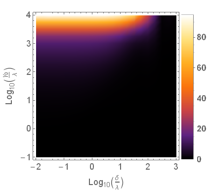
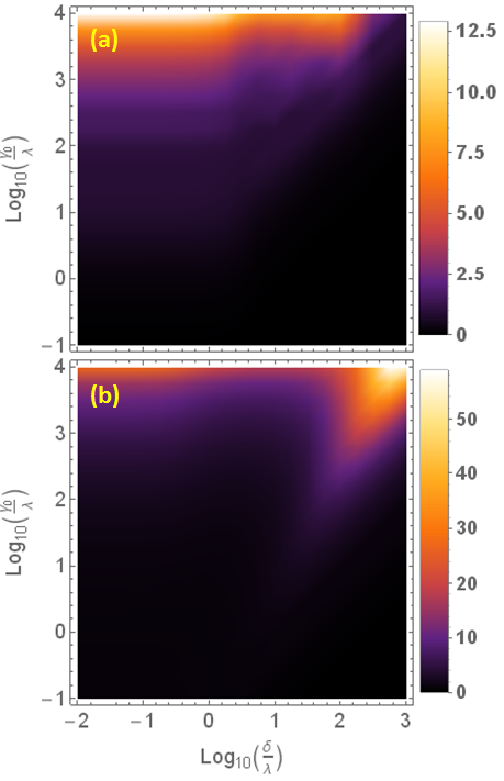
For a general process the maximisation over the initial states, and , in , is a difficult task. However for the DJC model considered here, when , it was shown in breuer that where and , with the eigenstates of the Pauli operator . In Fig.1 we show the behaviour of the measure as a function of the parameters and that control the DJC model.
IV Results: QSL bounds in the DJC model
The DJC model is a very suitable framework to analyse all the QSL bounds discussed in the previous Section. Our goal is to examine which of the bounds stay close to the essence of the QSL theory giving consistent estimates for the minimal evolution time to reach a final state from an initial one within the framework of open quantum evolutions.
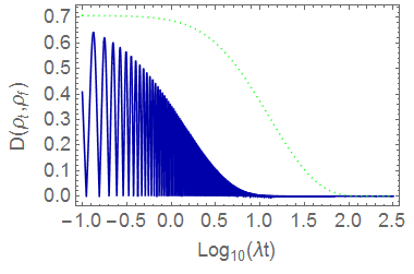
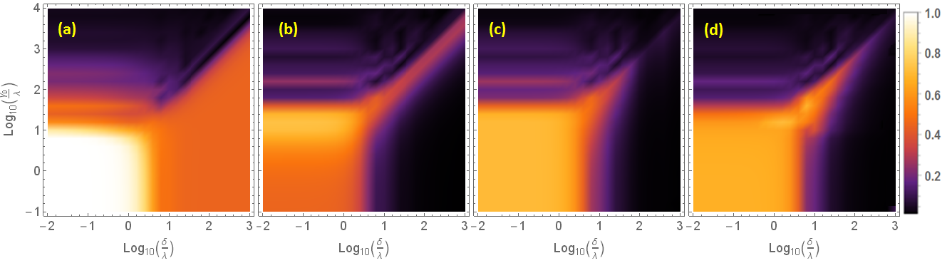
The reduced evolution of the qubit in the DJC model in Eq.(26) has a stationary state, for all values of the parameters and . Indeed, no matter which is the initial state and due to the fact that , the asymptotic final state is . The speed at which an evolved state approaches the stationary state is different in the Markovian and non-Markovian regimes. This is clearly shown in Fig.2 where we plot the trace distance, , between the evolved state of the qubit and its stationary state , as a function of time for two different parameters that controls the environment and its interaction with the qubit. The initial state is , however similar results were obtained from any other (not shown). We see that in the Markovian regime ( and ) the stationary state is reached for times , while in the non-Markovian regime ( and ) the final state is approached for earlier times (. This shows the speed up of the evolution in the non-Markovian regime.
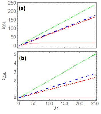
Let us now consider the behaviour of the different QSL bounds as a function of the final time of evolution shown in Fig.3. We remark that equivalent results were obtained for any other initial pure state (not shown). We can appreciate in Fig.3 that for times when, either in the Markovian and non-Markovian regime, the qubit have reached the stationary state (see Fig.(2)), only the bound remains constant. The other bounds grow approximately linear. This behavior is due to the fact that in the denominator of the definitions of , and (Eqs.(6), (14) and (22) respectively), appear the “average velocities" (with frequency units), , and , that depends on the actual evolution time . These average velocities go to zero when the stationary state is achieved while the quantities in the numerator of the definitions of the bounds remain constant. This is shown in Fig.4 where we plot , and , as a function of the evolution time , and we also plot that was defined in Eq. 5.
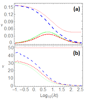
The results shown in Fig.3 and Fig.4 clearly show that none of the bounds, , and , give a consistent estimate of the minimal time to achieve the final state starting from the initial one . Moreover, the average velocities, , and , have the same asymptotic behavior as the instant speed of evolution, given by , that for also it goes to zero. This fact goes against the essence of the QSL theory that pursue the estimation of a speed limit velocity of the evolution between two states. On the contrary, gives a consistent estimate of the minimal time needed to reach from , and also provides a quantum speed limit of evolution.
Although we have shown that only one of the QSL bounds presented in Section II gives a reliable estimate of the minimum evolution time, we study now the connection of these bounds with the non-Markovianity character of the evolution deffner ; Sun2015 ; Meng2015 .
The measure in Eq.(33) is suitable to characterize the degree of non-Markovianity of a quantum channel . However, in order to establish a possible link between the QSL bounds and non-Markovian effects of the dynamics it is more appropriate to define a measure of non-Markovianity over the actual trajectory of the system i.e. from the initial state to the final one , that enters in the definition of the QSL bounds. In this way, we define
| (35) | |||||
that depends on the final time , and where
| (36) |
In Fig.(5) we show a density plot of as a function of the parameters and for an initial state and two final evolution times: (panel (a)) and (panel (b)). Comparing Fig.(1) and Fig.(5), we can see similar qualitative behaviour of the two measures of the non-Markovianity as a function of the two parameters, and , that controls the dynamics of the channel.
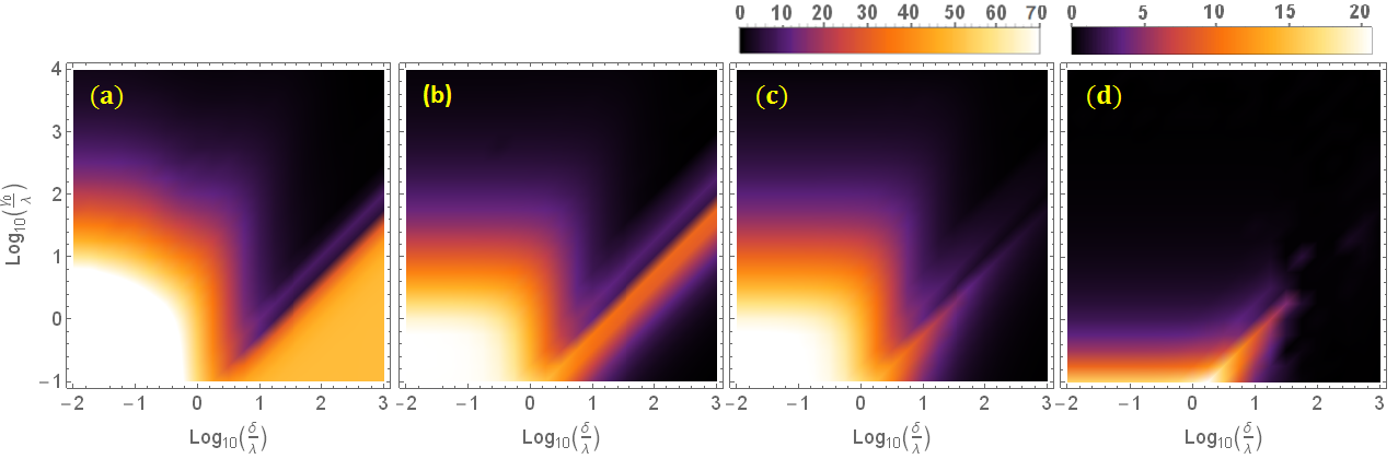
In order to compare the non-Markovianity measure with the QSL bounds we compute them for the same region of parameters and and also considering the initial state . In Fig. 6 we show the QSL bounds calculated for a final state at and in Fig. 7 for a final state at . The region of large in Fig.5 (a) corresponds to small values of all of the QSL bounds in Fig. 6. Same result can be observed comparing Fig. 5 (b) and Fig. 7. In this sense, large non-Markovianity implies small QSL bounds. This is a manifestation of the speed up of the quantum evolution in the non-Markovian regime that we have shown in Fig. 2. But looking at the value of the QSL bounds for different values of the parameters and , it is not possible to infer which are the parameter regions of non-Markovian behaviour of the channel. For example, the region of small values of the QSL bounds in the lower right corner in panels (b), (c), (d), and intermediate values in panel (a), of the Fig.6, do not correspond to the region of parameters with high values of the measure in Fig. 5 (a) . Exactly the same analysis can be done for the case of that are plotted in panel (b) of Fig.5 and Fig.7.
V Conclusions
Two quantum states are not perfect distinguishable unless their supports do not overlap. This makes that states that are close in Hilbert space are less distinguishable, so the distance between states fix the degree of distinguishability between them. Therefore, in order to connect with a physical evolution two states with some fix degree of distinguishability, it is necessary to at least go the same distance that separates the two states. This is the origin of the minimal time of evolution settled by quantum mechanics. The Quantum Speed Limit theory is devoted to establish lower bounds of this minimal time of evolution and its origin dates back to the pioneers works of Mandelstam & Tamm and Margolus & Levitin for unitary evolutions connecting pure states. It is important to note that the lost of the distinguishability between near neighbours states in quantum mechanics is intrinsic and has nothing to do with the precision of the measurement apparatus used to distinguish them. This contrasts with the classical case where the states of the system are given by points in the phase space, whose distinguishability is not related with the distance between them.
A reasonable requirement that any expression corresponding to a QSL bound for the minimal time of evolution between two states must satisfy is that if we apply the formula in the context of a given dynamics, the result must be close to the minimal time of evolution and not to the actual time of evolution between the states (unless the bound has been saturated). In this work we analysed the QSL bounds for the minimal time of evolution in open quantum systems taddei ; deffner ; jing , and have shown that only one, given in taddei , effectively verify this basic requirement. This was done using the damped Jaynes-Cummings model that for any initial state has the same stationary state. So, we have revealed that the QSL bounds in deffner ; jing grow indefinitely with the actual evolution time while the final state is essentially reached for finite times. On the contrary the QSL bound in taddei remains constant for any time greater that the time where the stationary state is essentially reached. We have also demonstrate that, contrary to the QSL bounds in taddei ; jing , the QSL bound in deffner can not be saturated continuously in time along a quantum evolution path.
In relation with the possible link between the non-Markovian effects and the behaviour of QSL bounds we found that all of the analysed bounds have lower values in a parameter region that match the parameter region where takes place the speed up of the quantum evolution due to non-Markovian effects in the damped Jaynes-Cummings model. However, we also have shown that there is a parameter region of lower values of all the analysed bounds that does not correspond to the region of non-Markovian effects on the evolution. In this sense, we have demonstrated, with a counterexample, that the statement that the non-Markovian effects on a quantum evolution can be study through the QSL bounds is false.
Acknowledgements.
FT acknowledge financial support from the Brazilian agencies CNPq, CAPES and the INCT-Informação Quântica. DAW acknowledge support from CONICET, UBACyT, and ANPCyT (Argentina). We are grateful to R. L. de Matos Filho, M. M. Taddei, C. Pineda and D. Davalos for fruitful discussions.References
- (1) J. D. Bekenstein, Phys. Rev. Lett. 46, 623 (1981).
- (2) S. Lloyd, Nature (London) 406, 1047 (2000).
- (3) V. Giovannetti, S. Lloyd, and L. Maccone, Nat. Photonics 5, 222 (2011).
- (4) M. Schosshauer, Decoherence and quantum to classical transition, Springer, Berlin/Heidelberg (2007).
- (5) Breuer H-P and F. Petruccione,The Theory of Open Quantum Systems, Oxford University Press, Oxford, UK, (2007).
- (6) M. M. Taddei, B. M. Escher, L. Davidovich, and R. L. de Matos Filho, Phys. Rev. Lett. 110, 050402 (2013).
- (7) S. Deffner, E. Lutz, Phys. Rev. Lett. 111, 010402 (2013).
- (8) L. Mandelstam and I. Tamm, J. Phys. USSR 9, 249 (1945).
- (9) N. Margolus and L. B. Levitin, Physica (Amsterdam) 120D, 188 (1998).
- (10) L. B. Levitin and T. Toffoli, Phys. Rev. Lett. 103, 160502 (2009).
- (11) V. Giovannetti, S. Lloyd and L. Maccone, Phys. Rev. A 67, 052109 (2003).
- (12) D. J. C. Bures, Trans. Am. Math. Soc. 135, 199 (1969).
- (13) Michael A. Nielsen and Isaac L. Chuang. 2011. Quantum Computation and Quantum Information: 10th Anniversary Edition (10th ed.). Cambridge University Press, New York, NY, USA.
- (14) R. Jozsa, J. Mod. Opt. 41, 2315 (1994).
- (15) Z. Sun, J. Liu, J. Ma, and X. Wang, Scientific Reports 5, 8444 (2015).
- (16) X. Meng, C. Wu, and H. Guo, Scientific Reports 5, 16357 (2015).
- (17) D. P. Pires, M. Cianciaruso, L. C. Céleri, G. Adesso, and D. O. Soares-Pinto, Phys. Rev. X 6, 021031 (2016).
- (18) S.-X. Wu, Y. Zhang, C.-S. Yu, and H.-S. Song, J Phys a-Math Theor 48, 045301 (2015).
- (19) J. Jing, L. A. Wu, A. del Campo, arXiv:1510.01106.
- (20) A. del Campo, I. L. Egusquiza, M. B. Plenio and S. F. Huelga Phys. Rev. Lett. 110, 050403 (2013).
- (21) D. P. Pires, M. Cianciaruso, L. C. Céleri, G. Adesso, and D. O. Soares-Pinto, Phys. Rev. X 6, 021031 (2016).
- (22) A. Uhlmann, in Quantum Groups and Related Topics: Proceedings of the First Max Born Symposium, edited by R. Gielerak, J. Lukierski, and Z. Popowicz (Kluwer Academic, Dordrecht, 1992), p. 267.
- (23) I. Marvian and D. A. Lidar, Physical Review Letters 115, 210402 (2015).
- (24) D. A. Lidar, P. Zanardi, and K. Khodjasteh, Physical Review A 78, 012308 (2008).
- (25) R. Uzdin and R. Koslof, arXiv:1607.00941 [quant-ph] (2016).
- (26) M. Sarovar and G. J. Milburn, J. Phys. A: Math. Gen., v. 39, 8487, 2006.
- (27) E. T. Jaynes and F. W. Cummings, Proc. IEEE 51, 89 (1963).
- (28) R. D. Grigorieff, Math. Nachr. 151, 327, (1991).
- (29) P. Breuer, J. Phys. B: At. Mol. Opt. Phys. 45, 154001 (2012).
- (30) P. Iyengar, G. N. Chandan, and R. Srikanth, arXiv:1312.1329v1.
- (31) L. Ferro, P. Facchi, R. Fazio, F. Illuminati, G. Marmo, V. Vedral, and S. Pascazio, arXiv:1501.03099v1.
- (32) H. P. Breuer, B. Kappler, and F. Petruccione, Phys. Rev. A 59, 1633 (1999).
- (33) B. M. Garraway, Phys. Rev. A 55, 2290 (1997).
- (34) Breuer H-P, Laine E-M and Piilo J, Phys. Rev. Lett. 103 210401, (2009).
- (35) Z. He, J. Zou, L. Li, and B. Shao, Phys Rev A 83, 012108 (2011).
- (36) B. Bylicka, D. Chruściński, and S. Maniscalco, Scientific Reports 4, (2014).
- (37) C. Pineda, T. Gorin, D. Davalos, D. A. Wisniacki, and I. García-Mata, Phys. Rev. A 93, 022117 (2016).