Star Formation Quenching Timescale of Central Galaxies in a Hierarchical Universe

Abstract

Central galaxies make up the majority of the galaxy population, including the majority of the quiescent population at $\mathcal{M}_{*}>10^{10}\mathrm{M}_{\odot}$. Thus, the mechanism(s) responsible for quenching central galaxies plays a crucial role in galaxy evolution as whole. We combine a high resolution cosmological $N$-body simulation with observed evolutionary trends of the “star formation main sequence,” quiescent fraction, and stellar mass function at $z<1$ to construct a model that statistically tracks the star formation histories and quenching of central galaxies. Comparing this model to the distribution of central galaxy star formation rates in a group catalog of the SDSS Data Release 7, we constrain the timescales over which physical processes cease star formation in central galaxies. Over the stellar mass range $10^{9.5}$ to $10^{11}\mathrm{M}_{\odot}$ we infer quenching e-folding times that span $1.5$ to $0.5\;\mathrm{Gyr}$ with more massive central galaxies quenching faster. For $\mathcal{M}_{*}=10^{10.5}\mathrm{M}_{\odot}$, this implies a total migration time of $\sim 4~{}\mathrm{Gyrs}$ from the star formation main sequence to quiescence. Compared to satellites, central galaxies take $\sim 2~{}\mathrm{Gyrs}$ longer to quench their star formation, suggesting that different mechanisms are responsible for quenching centrals versus satellites. Finally, the central galaxy quenching timescale we infer provides key constraints for proposed star formation quenching mechanisms. Our timescale is generally consistent with gas depletion timescales predicted by quenching through strangulation. However, the exact physical mechanism(s) responsible for this still remain unclear.

1. Introduction

Observations of galaxies using large galaxy surveys such as the Sloan Digital Sky Survey (SDSS; York et al. 2000), Cosmic Evolution Survey (COSMOS; Scoville et al. 2007), and the PRIsm MUlti-object Survey (PRIMUS; Coil et al. 2011; Cool et al. 2013) have firmly established a global view of galaxy properties out to $z\sim 1$. Galaxies are broadly divided into two main classes: star forming and quiescent. Star forming galaxies are blue in color, forming stars, and typically disk-like in morphology. Meanwhile quiescent galaxies are red in color, have little to no star formation, and typically have elliptical morphologies (Kauffmann et al. 2003; Blanton et al. 2003; Baldry et al. 2006; Wyder et al. 2007; Moustakas et al. 2013; for a recent review see Blanton & Moustakas 2009).

Over the period $z<1$, detailed observations of the stellar mass functions (SMF) reveal a significant decline in the number density of massive star forming galaxies accompanied by an increase in the number density of quiescent galaxies (Blanton 2006; Borch et al. 2006; Bundy et al. 2006; Moustakas et al. 2013). The growth of the quiescent fraction with cosmic time also reflects this change in galaxy population (Peng et al. 2010; Tinker et al. 2013; Hahn et al. 2015). Imprints of galaxy environment on the quiescent fraction (Hubble 1936; Oemler 1974; Dressler 1980; Hermit et al. 1996; for a recent review see Blanton & Moustakas 2009) suggest that there is a significant correlation between environment and the cessation of star formation. In comparison to the field, high density environments have a higher quiescent fraction. However, observations find quiescent galaxies in the field (Baldry et al. 2006; Tinker et al. 2011; Geha et al. 2012), at least for galaxies with stellar mass down to $10^{9}\mathrm{M}_{\odot}$ (Geha et al. 2012), and as Hahn et al. (2015) finds using PRIMUS, the quiescent fraction in both high density environments and the field increase significantly over time.

Furthermore, galaxy environment is a subjective and heterogeneously defined quantity in the literature (Muldrew et al. 2012). It can, however, be more objectively determined within the halo occupation context, which labels galaxies as ‘centrals’ and ‘satellites’ (Zheng et al. 2005; Weinmann et al. 2006; Blanton & Berlind 2007; Tinker et al. 2011). Central galaxies reside at the core of their host halos while satellite galaxies orbit around. During their infall, satellite galaxies are likely to experience environmentally driven mechanisms such as ram pressure stripping (Gunn & Gott 1972; Bekki 2009), strangulation (Larson et al. 1980; Balogh et al. 2000), or harassment (Moore et al. 1998).

Central galaxies, within this context, are thought to cease their star formation through internal processes – numerous mechanisms have been proposed and demonstrated on semi-analytic models (SAMs) and hydrodynamic simulations. One common proposal explains that hot gaseous coronae form in halos with masses above $\sim 10^{12}\mathrm{M}_{\odot}$ via virial shocks, which starve galaxies of cool gas required to fuel star formation (Birnboim & Dekel 2003; Kereš et al. 2005; Croton et al. 2006; Cattaneo et al. 2006; Dekel & Birnboim 2006). Other have proposed galaxy merger induced starbursts and subsequent supermassive blackhole growth as possible mechanisms (Springel et al. 2005; Di Matteo et al. 2005; Hopkins & Beacom 2006; Hopkins et al. 2008a, b). Feedback from accreting active galactic nuclei (AGN) has also been suggested to contribute to quenching (sometimes in conjunction with other mechanisms; Croton et al. 2006; Cattaneo et al. 2006; Gabor et al. 2011); so has internal morphological instabilities in the galactic disk or bar (Cole et al. 2000; Martig et al. 2009). With so many proposed mechanisms available, observational constraints are critical to test them.

Several works have utilized the observed global trends of galaxy populations in order to construct empirical models for galaxy star formation histories and quenching (e.g. Wetzel et al. 2013; Schawinski et al. 2014; Smethurst et al. 2015). Central galaxies constitute over $70\%$ of the $\mathcal{M}_{*}>10^{9.7}\mathrm{M}_{\odot}$ galaxy population at $z=0$. Moreover, the majority of the quiescent population at $\mathcal{M}_{*}>10^{10}\mathrm{M}_{\odot}$ become quiescent as centrals (Wetzel et al. 2013). The quenching of central galaxies plays a critical role in the evolution of massive galaxies. In this paper, we take a similar approach as Wetzel et al. (2013) but for central galaxies. Wetzel et al. (2013) quantify the star formation histories and quenching timescales in a statistical and empirical manner. Then using the observed SSFR distribution of satellite galaxies, they constrain the quenching timescale of satellites and illustrate the success of a “delay-then-rapid” quenching model, where a satellite begins to quench rapidly only after a significant delay time after it infalls onto its central halo.

Extending to centrals, we use the global trends of the central galaxy population at $z<1$ in order to construct a similarly statistical and empirical model for the star formation histories of central galaxies. While the initial conditions of the satellite galaxies in Wetzel et al. (2013) (at the times of their infall) are taken from observed trends of the central galaxy population, our model for central galaxies must actually reproduce all of the multifaceted observations. This requires us to construct a more comprehensive model that marries all the significant observational trends. Then by comparing the mock catalogs generated using our model to observations, we constrain the star formation histories and quenching timescales of central galaxies. Quantifying the timescales of the physical mechanisms that quench star formation, not only gives us a means for discerning the numerous different proposed mechanisms, but it also provides important insights into the overall evolution of galaxies.

We begin first in §2 by describing the observed central galaxy catalog at $z\approx 0$ that we construct from SDSS Data Release 7. Next, we describe the cosmological $N$-body simulation used to create a central galaxy mock catalog in §3. We then develop parameterizations of the observed global trends of the galaxy population and describe how we incorporate them into the mock catalog in §4. In §5, we describe how we use our model and the observed central galaxy catalog in order to infer the quenching timescale of central galaxies. Finally in §6 and §7 we discuss the implications of our results and summarize them.

2. Central Galaxies of SDSS DR7

We start by selecting a volume-limited sample of galaxies with $M_{r}-5\log(h)<-18$ from the NYU Value-Added Galaxy Catalog (VAGC; Blanton et al. 2005) of the Sloan Digital Sky Survey Data Release 7 (Abazajian et al. 2009) at redshift $z\approx 0.04$ following the sample selection of Tinker et al. (2011). The galaxy stellar masses are estimated using the $\mathtt{kcorrect}$ code (Blanton & Roweis 2007) assuming a Chabrier (2003) initial mass function (IMF). For measurement of galaxy star-formation, we use the specific star formation rate (SSFR) from the current release of Brinchmann et al. (2004) . Generally, SSFRs $\gtrsim 10^{-11}\mathrm{yr}^{-1}$ are derived from $\mathrm{H}\alpha$ emissions, $10^{-11}\gtrsim$ SSFRs $\gtrsim 10^{-12}\mathrm{yr}^{-1}$ are derived from a combination of emission lines, and SSFRs $\lesssim 10^{-12}\mathrm{yr}^{-1}$ are mainly based on $D_{n}4000$ (see discussion in Wetzel et al. 2013). The spectroscopically derived SSFRs, which accounts for dust-reddening, allow us to make more accurate distinctions between star-forming and quiescent galaxies than simple color cuts. We note that SSFRs $\lesssim 10^{-12}\mathrm{yr}^{-1}$ should only be considered upper limits to the true value (Salim et al. 2007).

Next, we identify the central galaxies using the halo-based group-finding algorithm from Tinker et al. (2011). For a detailed description we refer readers to Tinker et al. (2011); Wetzel et al. (2012, 2013, 2014), and Tinker et al. (2016). The most massive galaxy of the group is the ‘central’ galaxy and the rest are ‘satellite’ galaxies. In any group finding algorithm there are misassignments due to projection effects and redshift space distortions. Campbell et al. (2015), quantify both the purity and completeness of centrals identified using this group-finding algorithm at $\sim 80\%$. More importantly, they find that the algorithm can robustly identify red and blue centrals and satellites as a function of stellar mass and yield a nearly unbiased central red fraction, which is the key statistic relevant to our analysis here.

3. Simulated Central Galaxy Catalog

If we are to understand how central galaxies and their star formation evolve, we require simulations over a wide redshift range that allows us to examine and track central galaxies within the heirarchical growth of their host halos. To do this robustly, we require a cosmological N-body simulation that accounts for the complex dynamical processes that govern galaxy host halos. In this paper, we use the dissipationless, N-body simulation from Wetzel et al. (2013) generated using the White (2002) $\mathtt{TreePM}$ code with flat, $\Lambda$CDM cosmology: $\Omega_{\mathrm{m}}=0.274$, $\Omega_{\mathrm{b}}=0.0457$, $h=0.7$, $n=0.95$, and $\sigma_{8}=0.8$. $2048^{3}$ particles are evolved in a $250\;\mathrm{Mpc}/h$ box with particle mass of $1.98\times 10^{8}\mathrm{M}_{\odot}$ and with a Plummer equivalent smoothing of $2.5\;\mathrm{kpc}/h$. The initial conditions of the simulation at $z=150$ are generated using second-order Lagrangian Perturbation Theory. We refer readers to Wetzel et al. (2013) and Wetzel et al. (2014) for a more detailed description of the simulation.

From the $\mathtt{TreePM}$ simulation, Wetzel et al. (2013) identify ‘host halos’ using the Friends-of-Friends (FoF) algorithm of Davis et al. (1985) with linking length $b=0.168$ times the mean inter-particle spacing. This groups the simulation particles bound by an isodensity contour of $\sim 100\times$ the mean matter density. Within the identified host halos, the simulation identifies ‘subhalos’ as overdensities in phase space through a 6-dimensional FoF algorithm (White et al. 2010). Wetzel et al. (2013) then track the host halos and subhalos across the simulation outputs in order to build merger trees. Next, Wetzel et al. (2013) designate the most massive subhalo in a newly-formed host halo at a given simulation out as the ‘central’ subhalo. A subhalo remains central until it falls into a more massive host halo, at which point it becomes a ‘satellite’ subhalo. Each subhalo is also assigned a maximum mass $M_{\mathrm{peak}}$, the maximum host halo mass the subhalo has had in its history.

Using the Wetzel et al. (2013) simulation, we obtain a galaxy catalog from the subhalo catalog by assuming that galaxies reside at the centers of the subhalos and through subhalo abundance matching (SHAM; Vale & Ostriker 2006; Conroy et al. 2006; Yang et al. 2009; Wetzel et al. 2012; Leja et al. 2013; Wetzel et al. 2013, 2014) to assign them stellar masses. SHAM assumes a one-to-one mapping that preserves the rank ordering between subhalo $M_{\mathrm{peak}}$ and stellar mass, $\mathcal{M}_{*}$ of its galaxy: $n(>M_{\mathrm{peak}})=n(>\mathcal{M}_{*})$. Through SHAM, we can assign galaxy stellar masses to subhalos based on observed stellar mass function (SMF) at the redshifts of the simulation outputs. Galaxy stellar masses independently at each snapshot. This allows us to not only track the history of the subhalo, but also track the evolution of galaxy stellar masses through their SHAM stellar masses at each snapshot.

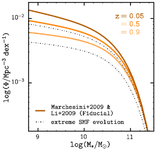
Figure 1.— The stellar mass function (SMF) that we use in our subhalo abundance matching (SHAM) prescription to construct galaxy catalogs from the Wetzel et al. (2013) $\mathtt{TreePM}$ simulation (§3). For our fiducial SMF (solid), we use the Li & White (2009) SMF at $z=0.05$ and interpolate between the Li & White (2009) SMF and the Marchesini et al. (2009) $z=1.6$ SMF for $z>0.05$. To illustrate the evolution, we plot the SMF at $z=0.05,0.5$, and $0.9$. We also plot a SMF parameterization using an “extreme” model of SMF evolution (dashed-dotted), in which the amplitude of the SMF at $z=1.2$ is half the amplitude of the fiducial SMF. We later use this extreme model to ensure that the results in this work remain robust over different degrees of SMF evolution at $z>0.05$.

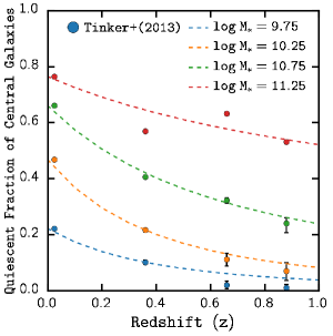
Figure 2.— The quiescent fraction of central galaxies, $f_{\mathrm{Q}}^{\mathrm{cen}}$, at $z<1$ in different stellar mass bins. We compare our parameterzation of $f_{\mathrm{Q}}^{\mathrm{cen}}$ (Eq. 2) using the best-fit parameter values listed in Table 1 (dashed) to the $f_{\mathrm{Q}}^{\mathrm{cen}}$ measurements from Tinker et al. (2013) (scatter). For our parameterization, we fit $f_{\mathrm{Q}}^{\mathrm{cen}}$ at $z=0.$ using central galaxies of the SDSS DR7 group catalog and fit $\alpha(\mathcal{M}_{*})$, which dictates the redshift dependence, from the redshift evolution of the Tinker et al. (2013) measurements.

For our SHAM prescription, we use the SMF of Li & White (2009) at the lowest redshift $z=0.05$. Li & White (2009) is based on the same SDSS NYU-VAGC sample as the SDSS DR7 group catalog we describe in §2. At higher redshifts, we interpolate between the Li & White (2009) SMF and the Marchesini et al. (2009) SMF at $z=1.6$ to obtain the SMF at the simulation output redshifts. This produces SMFs that increase significantly and monotonically over $z<1$ for $\mathcal{M}_{*}<10^{11}\mathrm{M}_{\odot}$ but insignificantly for $\mathcal{M}_{*}>10^{11}\mathrm{M}_{\odot}$. We choose the Marchesini et al. (2009) SMF, amongst others, because it produces interpolated SMFs that monotonically increase at $z<1$. At $z\sim 1$, the interpolated SMF we use is consistent (within the $1\sigma$ uncertainties) with more recent measurements from Muzzin et al. (2013) and Ilbert et al. (2013).

In Figure 1, we illustrate the evolution of the SMFs that we use for our SHAM prescription (solid) for $z=0.05,0.5$, and $0.9$. Recently, using PRIMUS, Moustakas et al. (2013) found little evolution in the SMF for $z<1$ at all mass ranges. Although previous works such as Bundy et al. (2006) find otherwise. To ensure that our results do not depend on our choice of the SMFs, later in §5.2, we repeat our analysis using SMFs with no evolution (i.e. Li & White 2009 SMF throughout $0<z<1$) and with “extreme” evolution for $z>0.05$ (dash-dotted in Figure 1), in which the amplitude of the SMF at $z=1.2$ is approximately half the amplitude of the fiducial SMF at $z=1.2$. Furthermore, while the simplest version of SHAM assumes a one-to-one correspondence between $M_{\mathrm{peak}}$ and $\mathcal{M}_{*}$, observations suggest that there is a scatter of $\sim 0.2\;\mathrm{dex}$ in this relation (Zheng et al. 2007; Yang et al. 2008; More et al. 2009; Gu et al. 2016). Hence, we apply a $0.2\;\mathrm{dex}$ log-normal scatter in $\mathcal{M}_{*}$ at fixed $M_{\mathrm{peak}}$ in our SHAM prescription at each snapshot independently.

So far, we have subhalos populated with galaxies and their stellar mass at each of the $15$ simulation outputs spanning the redshift $0.05<z<1$. For our sample, we restrict ourselves to galaxies classified as centrals by the simulation. And also to ones that are in both the $z\sim 0.05$ and $z\sim 1$ snapshots. This removes $<3\%$ of central galaxies with $\mathcal{M}_{*}>10^{9.5}~{}\mathrm{M}_{\odot}$ in the $z\sim 0.05$ snapshot. Our sample inevitably includes “back splash” or “ejected” satellite galaxies (Wetzel et al., 2014), misclassified as centrals. Excluding these galaxies, however, has a negligible impact on our results. We also note that while we do not have an explicit prescription for stellar mass growth from mergers, based on SHAM, the stellar mass growth traces the merger induced subhalo growth. As we discuss later in detail, mounting evidence disfavor merger driven quenching as the trigger of star formation quenching, so our treatment of mergers do not impact our quenching timescale results. In summary, we construct from our simulation a catalog of central galaxies whose stellar mass and halo mass is be traced through the redshift range $0.05<z<1$.

4. Star Formation in Central Galaxies

The $\mathtt{TreePM}$ simulation (§3) provides a framework to examine the evolution of central galaxies within the $\Lambda$CDM hierarchical structure formation of the Universe. In order to determine the quenching timescale of central galaxies, we incorporate the evolution of star-formation within this framework so that the star formation of the simulated central galaxies reproduce observed trends. More specifically, we implement star formation in central galaxies to reproduce the observed evolution of the quiescent fraction and star-forming main sequence.

We begin in §4.1 by describing our paramertization of the observed quiescent fraction and SFMS evolutionary trends at $z<1$. Afterwards, we describe the initial SFR assignment of the central galaxies in the simulation at the $z=1$ snapshot in §4.2. Then in §4.3 we describe how our model evolves the SFRs and quenches these central galaxies.

4.1. Observations

With galaxy surveys like the SDSS, COSMOS, and PRIMUS, observations have firmly established that for $z<2$, galactic properties such as color and star formation rate (SFR) have a bimodal distribution (Baldry et al. 2006; Cooper et al. 2007; Blanton & Moustakas 2009; Moustakas et al. 2013). As mentioned above, the two main components of this distribution are quiescent galaxies with little star formation, which are redder, more massive, and reside in denser environments and star forming galaxies, which are bluer, less massive and more often found in the field. Since this bimodality is most likely a result of star formation being quenched in galaxies, measurements of the quiescent fraction $f_{\mathrm{Q}}$, the fraction of quiescent galaxies in a population, is often used to indicate the overall star-forming property of galaxy populations (Baldry et al. 2006; Drory et al. 2009; Cooper et al. 2010; Iovino et al. 2010; Peng et al. 2010; Geha et al. 2012; Kovač et al. 2014; Hahn et al. 2015).

For $z<1$, observations find that the overall quiescent fraction increases as a function of stellar mass and with lower redshift (Drory et al. 2009; Iovino et al. 2010; Peng et al. 2010; Kovač et al. 2014; Hahn et al. 2015). In Wetzel et al. (2013), they quantify this mass and redshift dependence of the quiescent fraction through the parameterization, $f_{\mathrm{Q}}(\mathcal{M}_{*},z)=A(\mathcal{M}_{*})\times(1+z)^{\alpha(\mathcal{M}_{*})}$, with $A(\mathcal{M}_{*})$ and $\alpha(\mathcal{M}_{*})$ fit from the quiescent fractions of the SDSS DR 7 catalog and the COSMOS survey at $z<1$ (Drory et al. 2009), respectively. However, the quiescent fraction evolution is not universal over all environments (Hahn et al. 2015). More specifically, Tinker & Wetzel (2010) and Tinker et al. (2013) find distinct quiescent fraction evolutions for central and satellite galaxies.

We focus solely on the central galaxy quiescent fraction. We use the same parameterization as the overall quiescent fraction parameterization in Wetzel et al. (2013):

$$f_{\mathrm{Q}}^{\mathrm{cen}}(\mathcal{M}_{*},z)=f_{\mathrm{Q}}^{\mathrm{cen}}(\mathcal{M}_{*},z=0)\times(1+z)^{\alpha(\mathcal{M}_{*})}$$ (1)

where

$$f_{\mathrm{Q}}^{\mathrm{cen}}(\mathcal{M}_{*},z=0.)=A_{0}+A_{1}\;\log\mathcal{M}_{*},$$ (2)

is fit to the SDSS DR7 group catalog central galaxies (§2). $\alpha(\mathcal{M}_{*})$, which dictates the redshift dependence of Eq. 1, is fit using the redshift dependence of $f_{\mathrm{Q}}^{\mathrm{cen}}$ measurements from Tinker et al. (2013), derived from observations of the SMF, galaxy clustering, and galaxy-galaxy lensing within the COSMOS survey, in bins of width $\Delta\log\mathcal{M}_{*}=0.5\;\mathrm{dex}$. In Table 1, we list the best fit values for the parameters in Eq. 1 and in Figure 2 we compare our parameterization to the Tinker et al. (2013) measurements.

Observations of galaxy populations also find a tight correlation between the SFRs of star-forming galaxies and their stellar masses, which is referred to in the literature as the “star formation main sequence” (SFMS; Noeske et al. 2007; Oliver et al. 2010; Karim et al. 2011; Moustakas et al. 2013). Star-forming galaxies with higher stellar masses have higher SFRs. Roughly, this mass dependence can be characterized by a power law, $\mathrm{SFR}\propto\mathcal{M}^{\beta}$ and for a given stellar mass, SFRs follows a log-normal distribution (Noeske et al. 2007; Lee et al. 2015). Over cosmic time, this tight correlation decreases in SFR but has a constant scatter with $\sigma_{\log\mathrm{SFR}}\sim 0.3\;\mathrm{dex}$ (Noeske et al. 2007; Elbaz et al. 2007; Daddi et al. 2007; Salim et al. 2007; Whitaker et al. 2012; Lee et al. 2015), In fact this decline SFR of star-forming galaxies in the SFMS is likely responsible for the remarkable decline of star formation in the Universe (Hopkins & Beacom 2006; Behroozi et al. 2013; Madau & Dickinson 2014).

Following the typical power-law parameterization of the SFMS, we construct a flexible parameterization that depends on mass and redshift. For a given stellar mass and redshift, the mean SFR of the SFMS is given by

$$\overline{\raisebox{0.0pt}[1.2pt]{SFR}}_{\mathrm{MS}}(\mathcal{M}_{*},z)=A_{\mathrm{SDSS}}\left(\frac{\mathcal{M}_{*}}{10^{10.5}\mathrm{M}_{\odot}}\right)^{\beta_{\mathcal{M}}}10^{\beta_{z}(z-0.05)}.$$ (3)

$A_{\mathrm{SDSS}}$ is the SFR of the SFMS for the SDSS group catalog at $\mathcal{M}_{*}=10^{10.5}\mathrm{M}_{\odot}$. We determine $\beta_{\mathcal{M}}$ from fitting Eq. 3 to the SFMS of the SDSS group catalog ($z=0.05$). Then we determine $\beta_{z}$ such that the redshift dependence of our estimate of cosmic star formation rate,

$$\rho_{\mathrm{SFR}}(z)\propto\int\left(1-f^{\mathrm{cen}}_{\mathrm{Q}}\right)\mathrm{SFR}_{\mathrm{MS}}(\mathcal{M},z)\Phi(\mathcal{M},z)\;\mathrm{d}\mathcal{M},$$ (4)

is consistent with the redshift dependence of the cosmic star formation rate observations at $z<1$ (Behroozi et al. 2013). $\Phi(\mathcal{M},z)$ and $f_{\mathrm{Q}}^{\mathrm{cen}}$ in Eq. 4, are the SMF used in the SHAM procedure (§3) and the central galaxy quiescent fraction (Eq. 1). This agreement in redshift dependence ensures the observational consistency between the SMF and the cosmic star formation density evolution, which Behroozi et al. (2013) find. We list the best fit values to $A_{\mathrm{SDSS}},\beta_{\mathcal{M}}$, and $\beta_{z}$ in Table 1. Our $\beta_{\mathcal{M}}$ and $\beta_{z}$ values are consistent with similar parameterizations in the literature (Salim et al. 2007; Moustakas et al. 2013; Lee et al. 2015).

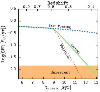
Figure 3.— Schematic diagram that illustrate the star formation evolution of central galaxies in our model (§4.3). We plot SFR as a function of $t_{\mathrm{cosmic}}$ for a star forming galaxy (blue dashed), a star-forming galaxy that quenches at $t_{\mathrm{Q,start}}=9\;\mathrm{Gyr}$ (green) and mark the general region of quiescent galaxies (orange). Central galaxies while they are star-forming have SFRs that evolve with the SFMS, which decreases with cosmic time. When star-forming central galaxies quench, their SFR decreases exponentially with $t_{\mathrm{cosmic}}$. The quenching timescale, $\tau_{\mathrm{Q}}^{\mathrm{cen}}$, we constrain in our analysis dictates how rapidly these galaxies quench based on Eq. 8. For comparison we also plot the SFR evolution of a satellite with the same mass using the Wetzel et al. (2013) quenching timescales (red dashed).

4.2. Assigning Star Formation Rates

The first output of the $\mathtt{TreePM}$ simulation that we utilize is at $z_{\mathrm{initial}}=1.08$. We designate the central galaxies of this snapshot as quenching, star-forming or quiescent and assign SFRs to them as the initial conditions of our model. The SFR assignment are based on the observed galaxy bimodality, the SFMS, and quiescent fraction at $z_{\mathrm{initial}}$ as we detail below.

First, we classify a fraction of the central galaxies as “quenching” galaxies – galaxies that reside in the green valley, which are in the transitional state of becoming quiescent from star-forming. Current observations do not provide strong constraints on the fraction of galaxies “quenching” at $z\sim 1$. So, we use a flexible and mass dependent prescription

$$f_{GV}(\mathcal{M}_{*})=A_{GV}(\log\;\mathcal{M}_{*}-10.5)+\delta_{GV}$$ (5)

and marginalize over the nuisance parameters, $A_{GV}$ and $\delta_{GV}$, in our analysis. For these designated quenching central galaxies, we assign SFRs by uniformly sampling between the average SFR of the SFMS (Eq. 3) at $z_{\mathrm{initial}}$ and $\mathrm{SFR}_{\mathrm{Q}}(\mathcal{M}_{*})$, the SFR of the quiescent peak of the SDSS central galaxy SSFR distribution, which we later detail in this section.

Next, we classify the remaining $1-f_{\mathrm{GV}}$ of the galaxy population as either star-forming or quiescent to match $f_{\mathrm{Q}}^{\mathrm{cen}}(z=z_{\mathrm{initial}})$. Galaxies classified as star-forming, are assigned SFRs based on the log normal SFR distribution of the SFMS at $z_{\mathrm{initial}}$ with scatter $\sigma_{\log\mathrm{SFR}}\sim 0.3$ (§4.1):

$$\log\mathrm{SFR}_{\mathrm{SF}}^{init}=\mathcal{N}(\log\overline{\raisebox{0.0pt}[1.2pt]{SFR}}_{\mathrm{MS}}\left(\mathcal{M}_{*},z_{\mathrm{initial}}),\;0.3\right).$$ (6)

where $\mathcal{N}$ represents a Gaussian. Galaxies classified as quiescent are assigned SFRs based on a log-normal distribution centered about $\overline{\raisebox{0.0pt}[1.2pt]{SFR}}_{\mathrm{Q},init}$ with scatter $\sigma_{\log\mathrm{SFR}}^{\mathrm{Q}}$:

$$\log\mathrm{SFR}_{\mathrm{Q}}^{init}=\mathcal{N}(\overline{\raisebox{0.0pt}[1.2pt]{SFR}}_{\mathrm{Q},init},\sigma_{\log\mathrm{SFR}}^{\mathrm{Q}})$$ (7)

Both $\overline{\raisebox{0.0pt}[1.2pt]{SFR}}_{\mathrm{Q},init}$ and $\sigma_{\log\mathrm{SFR}}^{\mathrm{Q}}$ are determined empirically from the quiescent peak SSFR in the SDSS central galaxy SSFR distribution: $\overline{\raisebox{0.0pt}[1.2pt]{SFR}}_{\mathrm{Q},init}=0.4\;(\log\mathcal{M}_{*}-10.5)-1.73$ and $\sigma_{\log\mathrm{SFR}}^{\mathrm{Q}}=0.18$. Our aim is solely to empirically reproduce the quiescent peak because the SSFR measurements are largely upper limits, so the peak itself is nonphysical (§2).

4.3. Star Formation Evolution

Starting from the initial SFRs of the central galaxies that we just assigned, next, we evolve the SFRs in order to reproduce the observed evolution of the quiescent fraction and the SFMS (§4.1). The central galaxies in our simulation evolve their SFRs as star-forming galaxies, quiescent galaxies and quench their star-formation. With the focus of this work on the quenching timescale of central galaxies, we first discuss how we evolve the SFRs of central galaxies that quench within our simulation. Then we discuss how we evolve the SFRs of central galaxies while they are star-forming and after they have quenched their star formation.

Once a galaxy begins to quench its star formation, its SFR decreases and, on the SFR-$\mathcal{M}_{*}$ relation, it migrates from the SFMS to the quenched sequence. We designate the time when a galaxy starts to quench as $t_{Q,\mathrm{start}}$ and model its decline in SFR exponentially with a characteristic e-folding time $\tau_{Q}^{\mathrm{cen}}$, which we refer to as the “central quenching timescale”:

$$\mathrm{SFR}_{\mathrm{Quenching}}(t)=\mathrm{SFR}_{\mathrm{SF}}(t)\times\exp\left(-\frac{t-t_{Q,\mathrm{start}}}{\tau^{\mathrm{cen}}_{Q}}\right).$$ (8)

$\mathrm{SFR}_{\mathrm{SF}}$ represents the SFR of a star-forming central galaxy, which we define later, and $\tau_{Q}^{\mathrm{cen}}$ characterizes how long quenching mechanism(s) take(s) to cease star-formation in a central galaxy. In order to determine whether this timescale depends on the stellar mass of the galaxy, we include a mass dependence:

$$\tau_{Q}^{\mathrm{cen}}(\mathcal{M}_{*})=A_{\tau}\left(\log\;\mathcal{M}_{*}-11.1\right)+\delta_{\tau}.$$ (9)

In addition to the SFR evolution after they begin to quench, our model must also quantify when and how many star-forming centrals quench from $z_{\mathrm{initial}}$.

For satellite galaxies, the moment they start quenching can be related to the the moment when their host halo is accreted into the central galaxy’s host halo via a time delay of several Gyrs (Wetzel et al. 2013). However, for central galaxies, the time when they start to quench is likely characterized by more complex and stochastic mechanisms such as gas depletion from strangulation (Peng et al. 2015), hot gas quenching (Gabor et al. 2010; Gabor & Davé 2012, 2015) or the onset of AGN activity. Fortunately, using the evolution of the quiescent fraction, we can statistically model the number of star-forming centrals that quenches throughout the simulation. We use a Monte Carlo prescription that utilizes a “quenching probability” ($P_{Q}$) to determine which star-forming centrals to quench and when to quench them. We define $P_{Q}$, for a stellar mass $\mathcal{M}_{*}$ at simulation snapshot $i$ as

$$P_{Q}(\mathcal{M}_{*},t_{i})=\frac{N_{Q}(\mathcal{M}_{*},t_{i+1})-N_{Q}(\mathcal{M}_{*},t_{i})}{N_{SF}(\mathcal{M}_{*},t_{i})}$$ (10)

where $N_{Q}(\mathcal{M}_{*},t)$ and $N_{SF}(\mathcal{M}_{*},t)$ represent the number of quiescent and star-forming galaxies of stellar mass $\mathcal{M}_{*}$ in the population at $t$.

In the fiducial case where quenching happens instantaneously and the time evolution of the stellar mass function is negligible, the quenching probability is given directly by the derivative of the quiescent fraction over time:

$$P^{fid}_{Q}(\mathcal{M},t_{i})=\frac{t_{i+1}-t_{i}}{1-f_{\mathrm{Q}}(\mathcal{M},t_{i})}\frac{\mathrm{d}f_{\mathrm{Q}}}{\mathrm{d}t}.$$ (11)

However, to account for the SMF evolution, we introduce a correction to Eq. 11:

$$\Delta P_{Q}(\mathcal{M},t_{i})=\frac{N_{\mathrm{tot}}(\mathcal{M},t_{i+1})-N_{\mathrm{tot}}(\mathcal{M},t_{i})}{N_{SF}(\mathcal{M},t_{i})}f_{Q}(\mathcal{M},t_{i+1}).$$ (12)

Furthermore, star-forming galaxies do not quench instantaneously. This implies that some galaxies can begin their quenching but still have high enough SFRs to be misclassified as star-forming causing a discrepancy between when star-forming galaxies start quenching to when they become classified as quiescent. This discrepancy depends on the SFRs of the quenching galaxies and the timescales of the quenching mechanism. Our ultimate goal is to characterize this timescale and its dependence on stellar mass, so any strong assumptions may bias our results. Therefore, we include a flexible mass dependent factor parameterized by $A_{P_{Q}}$ and $\delta_{P_{Q}}$ to the quenching probability prescription:

$$f_{P_{Q}}(\mathcal{M})=A_{P_{Q}}(\log\mathcal{M}-10.5)+\delta_{P_{Q}}.$$ (13)

By including this term to the quenching probability, we treat $A_{P_{Q}}$ and $\delta_{P_{Q}}$ as nuisance parameters, which mitigate any biases. Combined, the quenching probability we use is

$$P_{Q,i}(\mathcal{M})=f_{P_{Q}}\left(P^{fid}_{Q,i}+\Delta P_{Q,i}\right).$$ (14)

Later in §5.2 we discuss the potential impact of our quenching probability parameterization on our results. In practice, at each simulation output snapshot $t_{i}$, a number of star-forming central galaxies are selected to start quenching based on their assigned quenching probabilities. We note that our quenching probability prescription quenches star-forming galaxies anywhere on the SFMS.

For quenching galaxies before they start quenching and for star-forming galaxies that remain star-forming throughout, their star formation histories are dictated by the evolution of the SFMS. Therefore, we model the star formation evolution of star-forming central galaxies to statistically trace the redshift and mass dependence of the SFMS. Recall that the stellar masses of the central galaxies evolve independently from their star formation histories. Through our SHAM prescription, the stellar mass growth traces the mass accretion of its host subhalo (§ 3). Then, for a star-forming central with initial stellar mass $\mathcal{M}_{0}$ at $z_{\mathrm{initial}}$ that evolves to $\mathcal{M}$ at $z$ to remain on the SFMS, based on Eq. (3), the SFR at $z_{\mathrm{initial}}$ must evolve by the following factor

$$f_{\mathrm{MS}}=\left(\frac{\mathcal{M}}{\mathcal{M}_{0}}\right)^{\beta_{\mathcal{M}}}\times 10^{\beta_{z}(z-z_{0})}$$ (15)

where $\beta_{\mathcal{M}}$ and $\beta_{z}$ are the fixed parameters that characterize the mass and redshift dependence of the SFMS (§ 4.1 and Table 1). So while central galaxies with $\mathrm{SFR}_{0}$ at $z_{\mathrm{initial}}$ remain star-forming they have,

$$\mathrm{SFR}_{\mathrm{SF}}=f_{\mathrm{MS}}\times\mathrm{SFR}_{0}.$$ (16)

This way, star-forming galaxies follow the observed redshift evolution and mass dependence of the SFMS. Furthermore, since our prescription keeps the relative positions in SFR from $\overline{\raisebox{0.0pt}[1.2pt]{SFR}}_{\mathrm{MS}}$ constant, it preserve the SFR scatter of the SFMS – matching observations.

Of course, in reality, the SFHs of star-forming central galaxies do not strictly follow a simple parameterization of the SFMS evolution. The stellar mass growth of the star-forming centrals is not only related to the growth of its host subhalo, as our SHAM prescription assumes, but also linked to their SFHs. Observations, however, suggest a non-trivial connection between stellar mass growth, SFH, and host subhalo growth. For instance, if we estimate the stellar masses of star forming galaxy by integrating SFRs over time, then the stellar mass growth of star-forming galaxies with the same initial stellar mass but different SFR on the SFMS, would diverge over time and the final stellar masses will be significantly different. In that case, it would be difficult to preserve the SFR scatter in SFMS along with its log-normal characteristic. Alternatively, if independent of subhalo growth, the SFH linked stellar mass growth would cause the stellar mass growth for fixed halo mass to diverge. This would violate the observed scatter in the Stellar Mass to Halo Mass (SMHM) relation (Leauthaud et al., 2012; Tinker et al., 2013; Zu & Mandelbaum, 2015; Gu et al., 2016). Clearly a mechanism such as a “star formation duty cycle” is required to consolidate observations of the SMHM and the SFMS. For the scope of this paper, however, we find that our above prescription of statistically evolving the SFRs of star-forming galaxies is sufficient and incorporating stellar mass growth through integrated SFR with a stochastic star forming duty cycle, does not significant impact the constraints on the quenching timescales. We will investigate star formation duty cycle in star-forming central galaxies and the link between stellar mass growth, host halo growth and SFH in Hahn et al. in prep.

Lastly, central galaxies that are quiescent at $z_{\mathrm{initial}}$ or become quiescent during the simulation remain quiescent. Their SFR evolution is determined only to empirically reproduce the quiescent peak of the SSFR distribution at $z=0.05$, similar to the initial SFR assignment in §4.2. For galaxies that are quiescent at $z_{\mathrm{initial}}$, we evolve the SFRs in order to conserve the SSFRs throughout the simulation: $\mathrm{SSFR}_{\mathrm{Q}}=\mathrm{SSFR}_{0}$, the initial SSFR at $z_{\mathrm{initial}}$. Then,

$$\mathrm{SFR}_{\mathrm{Q}}=\mathrm{SSFR}_{0}\times\mathcal{M}_{*}$$ (17)

where $\mathcal{M}_{*}$ is stellar mass at the simulation outputs derived from SHAM. For galaxies that become quiescent through quenching during the simulation, based on Eq. 8 their SFRs can decrease significantly enough that their SSFRs falls below the lower bound of the SDSS DR7 SSFR measurements. Since we later compare the SSFR distribution of our model to the SSFR distribution of the SDSS DR7 central galaxy catalog, the quenching galaxies whose SFRs fall below the SDSS lower bound will bias the comparison. Therefore, we impose a final quenched SSFR assigned based the quiescent peak of the observed SSFR distribution for each galaxy when it begins to quench. The SFR of quenching galaxies only decreases until this final quenched SSFR. Afterwards, the SFR is evolved to conserve the SSFR (Eq. 17).

Figure 3 qualitatively illustrates the SFR evolution of star-forming (blue dashed), quenching (green solid), and quiescent (orange) central galaxies as a function of cosmic time throughout the simulation. The SFR of star-forming galaxies reflects the SFR evolution of the SFMS which decreases with time. The quenching galaxy starts to quench at at $t_{\mathrm{Q,start}}=9\;\mathrm{Gyr}$. Its departure from the SFMS is clearly illustrated at $t_{\mathrm{cosmic}}>9\;\mathrm{Gyr}$. The slope of its SFR decline is dictated by the quenching timescale. Since the lower bound of the SSFR in the SDSS group catalog does not have any physical significance, we broadly mark the region with $\log\;\mathrm{SSFR}<\log\;\mathrm{SSFR}_{\mathrm{Q}}+\sigma^{\mathrm{Q}}_{\log\;\mathrm{SFR}}$ as quiescent in Figure 3.

More quantitatively, in the top panel of Figure 4 we present the evolution of the SSFR distribution in our model (for a reasonable set of model parameter values) to illustrate how we track the star formation of central galaxies from $z\sim 1$. For this particular set of model parameter values, $f_{GV}\sim 0$ within the stellar mass bin. We plot the SSFR distribution for central galaxies in the stellar mass range $[10^{10.1}\mathrm{M}_{\odot},10^{10.5}\mathrm{M}_{\odot}]$ for a number of simulation output snapshots in the redshift range $0<z<1$ (top; darker with time). It demonstrates how our model reproduces the observed evolution of the SFMS and quiescent fraction. With time, the star-forming peak of the SSFR distribution decreases in SSFR tracing the SFMS evolution. The amplitude of the star-forming peak also decreases and is accompanied by the growth of the quiescent peak, reflecting the quiescent fraction evolution and the lower bound of SSFR measurements we impose.

In the bottom panel, we compare the SSFR distribution of our model at $z=0.05$ using a relatively shorter (dashed) and longer (dotted) quenching timescale than in the top panel (solid). The quenching timescale (parameterized by $A_{\tau}$ and $\delta_{\tau}$ in Eq. 9) dictates how long quenching central galaxies take to migrate from the SFMS to quiescence. The comparison illustrates that the length of the quenching timescale is reflected in the “height” of the SSFR distribution green valley. Longer quenching timescales, result in a higher green valley. Shorter quenching timescales, result in a lower one.

Table 1Parameterizations in the Central Galaxy SFH Model with Fixed Parameters

Parameter	Value
Central Galaxy Quiescent Fraction (Eq. 1)
$f_{\mathrm{Q}}^{\mathrm{cen}}(\mathcal{M}_{*},z)=f_{\mathrm{Q}}^{\mathrm{cen}}(\mathcal{M}_{*},z=0)\times(1+z)^{\alpha(\mathcal{M}_{*})}$
$\hskip 28.45274pt\hskip 28.45274pt\;\,=(A_{0}+A_{1}\log\mathcal{M}_{*})\times(1+z)^{\alpha(\mathcal{M}_{*})}$
8cm0.5pt3pt 2pt
$A_{0}$	$-6.04$
$A_{1}$	$0.64$
	$-2.57\quad\mathcal{M}_{*}\in[10^{9.5}-10^{10}\mathrm{M}_{\odot}]$
	$-2.52\quad\mathcal{M}_{*}\in[10^{10}-10^{10.5}\mathrm{M}_{\odot}]$
$\alpha(\mathcal{M}_{*})$	$-1.47\quad\mathcal{M}_{*}\in[10^{10.5}-10^{11}\mathrm{M}_{\odot}]$
	$-0.55\quad\mathcal{M}_{*}\in[10^{11}-10^{11.5}\mathrm{M}_{\odot}]$
	$-0.12\quad\mathcal{M}_{*}\in[10^{11.5}-10^{12}\mathrm{M}_{\odot}]$
SFMS SFR $z$ and $\mathcal{M}_{*}$ Dependence (Eq. 3)
$\overline{\raisebox{0.0pt}[1.2pt]{SFR}}_{\mathrm{MS}}=A_{\mathrm{SDSS}}\left(\frac{\mathcal{M}_{*}}{10^{10.5}\mathrm{M}_{\odot}}\right)^{\beta_{\mathcal{M}}}10^{\beta_{z}(z-0.05)}$
8cm0.5pt3pt 2pt
$A_{\mathrm{SDSS}}$	$10^{-0.11}\;\mathrm{M}_{\odot}/\mathrm{yr}$
$\beta_{\mathcal{M}}$	$0.53$
$\beta_{z}$	$1.1$

We list the parameters and their best-fit values for the central galaxy quiescent fraction (Eq. 1) and SFMS SFR redshift and stellar mass dependence (Eq. 3) parameterizations. $f_{\mathrm{Q}}^{\mathrm{cen}}(z=0)$ is fit using the central galaxies of the SDSS DR7 group catalog and the redshift dependence is fit using $f_{\mathrm{Q}}^{\mathrm{cen}}$ measurements from Tinker et al. (2013). Similarly, $\overline{\mathrm{SFR}}_{\mathrm{MS}}(z=0.05)$ is fit using the group catalog while the redshift dependence paramerization is fit to reproduce the redshift dependence of the Behroozi et al. (2013) cosmic star formation at $z<1$.

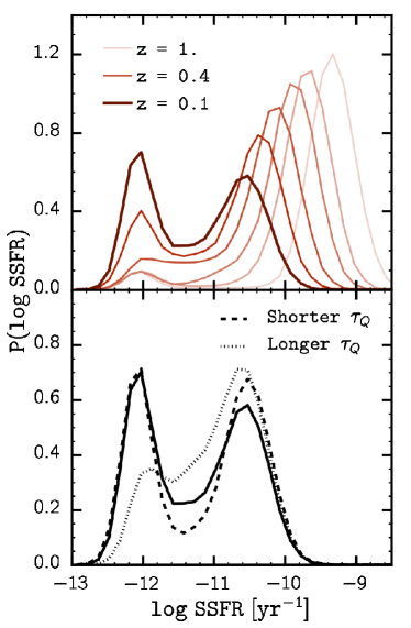
Figure 4.— Top: The evolution of the SSFR distribution in our model (§4.2) for a reasonable set of parameter values. The model evolves the SFR of central galaxies from $z\sim 1$ (light) to $0.05$ (dark) while reproducing the observed SFMS and quiescent fraction evolutions. The shift in the star forming peak of the SSFR distribution from $z=1$, reflects the overall decline in SFR of the SFMS over time. The quiescent fraction evolution is reflected in the growth of the quiescent peak accompanied by the decline of the star-forming peak. Bottom: Comparison of the SSFR distribution at $z=0.05$ using a relatively shorter (dashed) and longer (dotted) quenching timescale than the above panel (solid). The quenching timescale (parameterized by $A_{\tau}$ and $\delta_{\tau}$), dictates how long quenching central galaxies spend in between the peaks. This is ultimately reflected in the height of the green valley. For longer quenching timescales, the height of the SSFR distribution green valley will higher. For shorter quenching timescales, it will lower.

Table 2Parameterizations in the Central Galaxy SFH Model with Free Parameters

Quantity	Parameterization	Description	Parameter	Prior
$\tau_{Q}^{\mathrm{cen}}(\mathcal{M}_{*})$	$A_{\tau}(\log\;\mathcal{M}_{*}-11.1)+\delta_{\tau}$	Central Quenching Timescale in Gyrs (Eq. 9)	$A_{\tau}$	$[-1.5,0.5]$
			$\delta_{\tau}$	$[0.01,1.5]$
$f_{GV}(\mathcal{M}_{*})$	$A_{GV}(\log\;\mathcal{M}_{*}-10.5)+\delta_{GV}$	Initial $z\approx 1$ Green Valley Fraction (Eq. 5)	$A_{GV}$	$[0.,1.]$
			$\delta_{GV}$	$[-0.4,0.6]$
$f_{P_{Q}}(\mathcal{M}_{*})$	$A_{P_{Q}}(\log\mathcal{M}_{*}-10.5)+\delta_{P_{Q}}$	Quenching Probability Factor (Eq. 13)	$A_{P_{Q}}$	$[-5.,0.]$
			$\delta_{\tau}$	$[0.5,2.5]$

We list the parameterizations of the quenching timescale (Eq. 9), the initial $z\approx 1$ green valley fraction (Eq. 5), and the quenching probability factor (Eq.13) that we use in our model (§4). In our Approximate Bayesian Computation parameter inference, we constrain the parameters listed in the four column. For the prior probability distributions of these parameters, we use uniform priors with the ranges listed in the last column. We note that while we allow $\delta_{GV}<0$ due to the mass dependence of $f_{GV}$, $f_{GV}$ can only be non-negative in our model.

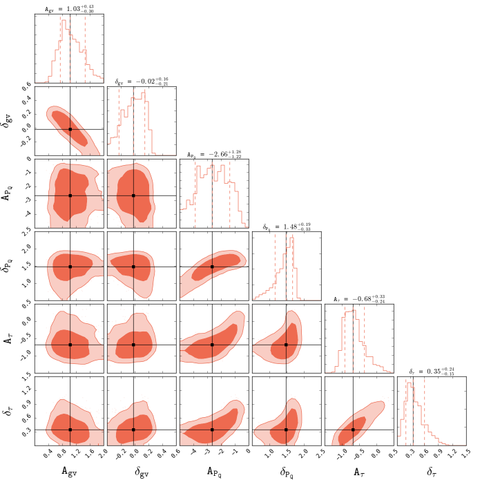
Figure 5.— We present the constraints we obtain for our model parameters using ABC-PMC. The diagonal panels plot posterior distributions of each of our model parameters, while the off-diagonal panels plot the degeneracies of parameter pairs. For each of the posterior distributions, we mark the $68\%$ confidence interval (vertical dashed lines). We also mark the median of the posterior distributions in all the panels in black.

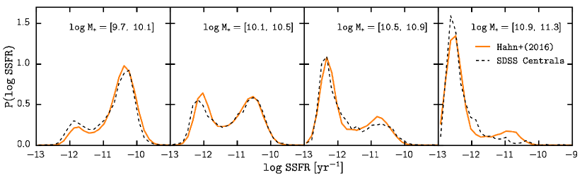
Figure 6.— Comparison between the SSFR distribution calculated using the median of the ABC posterior distribution as the set of model parameters (orange) and the SSFR distribution of the SDSS DR7 central galaxies (black dash). The SSFR distribution from the median of the ABC posterior show good overall agreement. The distributions are especially consistent in the transition (green valley) regions, which are dictated by the quenching timescale parameters.

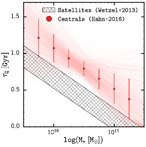
Figure 7.— Quenching timescale, $\tau_{\mathrm{Q}}^{\mathrm{cen}}$, of central galaxies (red) as a function of stellar mass. We plot $\tau_{\mathrm{Q}}^{\mathrm{cen}}$ of the median parameter values of the ABC posterior distributions (red points) along with $\tau_{\mathrm{Q}}^{\mathrm{cen}}$ drawn from the final iteration ABC parameter pool (faint red lines). For comparison, we also plot the satellite quenching timescale of Wetzel et al. (2014) (black dashed). The constraints we get for quenching timescale of central galaxies reveal that central galaxies have a significantly longer quenching timescale than satellite galaxies.

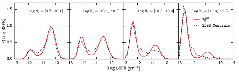
Figure 8.— The SSFR distribution generated from the median values of the parameter constraints obtained from our analysis using Wetzel et al. (2013) satellite quenching timescale as the quenching timescale of our central galaxies (red) in four stellar mass bins. In each panel, we reproduce the quiescent fraction of the SDSS DR7 central galaxies; however, comparison to the SSFR distribution of the SDSS DR7 centrals (black dash) find significant discrepancies in each of the bins. The SSFR distribution using satellite quenching timescale have much shallower green valley regions as a result of galaxies quenching much faster with satellite quenching timescale. This disagreement of model predictions for satellites applied to observations of centrals clearly demonstrates that centrals require longer quenching timescales than satellites.

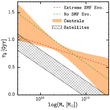
Figure 9.— Central galaxy quenching timescales ($\tau_{\mathrm{Q}}^{\mathrm{cen}}$) derived from using SMF prescriptions with no SMF evolution (green) and with extreme SMF evolution (red) in our analysis. For comparison we include the satellite galaxy quenching timescale from Wetzel et al. (2013) and $\tau_{\mathrm{Q}}^{\mathrm{cen}}$ we obtain using our fiducial SMF prescription. Even extreme choices for the SMF evolution is insufficient to account for the significant difference between the central and satellite quenching timescales. The different SMF evolution mainly impacts the mass dependence, not the amplitude of $\tau_{\mathrm{Q}}^{\mathrm{cen}}$.

5. Results

Now that we have a model for evolving star formation in central galaxies, in this section, we constrain the parameters of the model.

5.1. Approximate Bayesian Computation

Approximate Bayesian Computation (ABC) is a generative, simulation-based inference for robust parameter estimation. It has the advantage over standard approaches for parameter inference in that it does not require explicit knowledge of the likelihood function. It only relies on a simulation of observed data and on a metric for the distance between the observed data and simulation. It has already been effectively used for astronomy and cosmology in the literature (Cameron & Pettitt 2012; Weyant et al. 2013; Akeret et al. 2015; Ishida et al. 2015; Lin & Kilbinger 2015; Lin et al. 2016; Hahn et al. 2016, and Cisewski et al. in prep.), spanning a wide range of topics. For our purposes, which is to constrain the quenching timescale parameters, we use the observed SSFR distribution and quiescent fraction. ABC provides an ideal framework for parameter inference without having to specify the explicit likelihood of these observables. In practice, we use ABC in conjunction with the efficient Population Monte Carlo (PMC) importance sampling (Ishida et al. 2015; Hahn et al. 2016).

ABC requires a number of specific choices for implementation: a simulation of the data, a set of prior probability distributions for the model parameters, and a distance metric to compare the “closeness” of the simulation to the data. In §4, we described our model for the star formation evolution of central galaxies. The parameters of our model, which we constrain in our ABC analysis are listed in Table 2. For the prior probability distributions of the simulation parameters, $\{A_{\mathrm{GV}},\delta_{\mathrm{GV}},A_{P_{Q}},\delta_{P_{Q}},A_{\tau},\delta_{\tau}\}$, we choose uniform priors with conservative ranges also listed in Table 2.

The distance metric in ABC parameter estimation is — in principle — a positive definite function that compares various summary statistics between between the data and the simulation. It can be a vector with multiple components where each component is a distance between one particular summary statistic of the data and that of the simulation. For our case, the summary statistics we use for our distance metric are the observables we seek to reproduce with our model: the quiescent fraction evolution and SDSS DR7 central galaxy SSFR distribution. Therefore, we use a two component distance metric, $\vec{\rho}=[\rho_{\mathrm{QF}},\rho_{\mathrm{SSFR}}]$.

We calculate the first component, $\rho_{\mathrm{QF}}$, so that our model best reproduces the quiescent fraction at multiple snapshots:

$$\rho_{\mathrm{QF}}=\sum\limits_{\mathcal{M}}\sum\limits_{z^{\prime}\in\{z\}}\left(f^{\mathrm{cen}}_{\mathrm{Q}}(\mathcal{M},z^{\prime})-f^{\mathrm{model}}_{\mathrm{Q}}(\mathcal{M},z^{\prime})\right)^{2}$$ (18)

where $\{z\}=\{0.05,0.16,0.34$, and $1.08\}$ and $f^{\mathrm{cen}}_{\mathrm{Q}}$ is the parameterization of the observed quiescent fraction (Eq. 1. For $f^{\mathrm{model}}_{\mathrm{Q}}$ rather than using the actual evolutionary stages of the simulation central galaxies, we measure it using the following $\mathrm{SFR}-\mathcal{M}_{*}$ cut. The $\mathrm{SFR}-\mathcal{M}_{*}$ cut is derived from the slope of the SFMS relation (Eq. 3):

$$\log\;\mathrm{SFR}_{\mathrm{cut}}=\log\;\overline{\raisebox{0.0pt}[1.2pt]{SFR}}_{\mathrm{MS}}-0.9.$$ (19)

If a galaxy SFR is less than $\mathrm{SFR}_{\mathrm{cut}}$, then it is classified as quiescent; otherwise, as star-forming. This classification is analogous to the quiescent/star-forming classification of Moustakas et al. (2013), which also utilizes the slope of the SFMS. By measuring the quiescent fraction of the simulation we are more consistent with observations, which have no way of knowing the evolutionary stage of galaxies beyond their $\mathrm{SFR}$ and $\mathcal{M}_{*}$.

Our redshift choices for Eq. 18 is primarily motivated to ensure that our model agrees with the observed quiescent fraction throughout the lower redshifts ($z<0.5$). By incorporating the $z^{\prime}<0.5$ contributions, we constrain $A_{\mathrm{P_{Q}}}$ and $\tau_{\mathrm{P_{Q}}}$, which dictate the quenching probabilities. $z_{\mathrm{initial}}=1.08$ is also included to ensure that our initial conditions are consistent with observations.

The second component of our distance metric compares the SSFR distribution of the SDSS DR7 central galaxies to that of our model. More specifically,

$$\rho_{\mathrm{SSFR}}=\sum\limits_{\mathrm{SSFR}}\left(P(\mathrm{SSFR})^{\mathrm{SDSS}}-P(\mathrm{SSFR})^{\mathrm{model}}\right)^{2}.$$ (20)

As we discuss in § 4.3, the quenching timescale parameters leave an imprint on the SSFR distribution. So $\rho_{\mathrm{SSFR}}$ successfully serves to constrain $A_{\tau}$ and $\delta_{\tau}$.

Beyond our choice of distance metric, we strictly follow the ABC-PMC implementation of Hahn et al. (2016). For aficionados, we use a median distance threshold after each iteration of the PMC and declare convergence when the acceptance ratio falls below $1\%$. Once converged, the ABC algorithm produces parameter distributions that generate models with quiescent fractions and SSFR distributions close to observations. Moreover, these parameter distributions predict the posterior distributions of the parameters. For further details, we refer readers to Hahn et al. (2016).

5.2. Central Galaxy Quenching Timescale

We present the central galaxy quenching timescale constraints we obtain using ABC (§5.1), in Figure 5. The diagonal panels of the figure plot the posterior distribution of each of our model parameters with vertical dashed lines marking the median and the $68\%$ confidence interval. The off-diagonal panels plot the degeneracies between parameter pairs. We also mark the median of the posterior distribution for each of the parameters (black). The off-diagonal panels illustrate that the initial green valley parameters are not degenerate with the other parameters. Galaxies that are initially in the green valley quickly evolve out of it, so the green valley prescription is mainly constrained by the quiescent fraction at $z_{\mathrm{initial}}$. Furthermore, the off-diagonal panels that plot the degeneracies between the quenching probability parameters and the quenching timescale parameters exhibit expected correlation between the parameters: the longer the quenching timescale the larger the quenching probability correction factor ($f_{P_{Q}}$).

We compare the SSFR distribution generated from our model using the median model parameter values of the posterior distribution (orange) to the SSFR distribution of the SDSS DR7 central galaxy catalog (black dashed), in Figure 6. The SSFR distribution are computed for four stellar mass bins. We find good agreement between the SSFR distributions in each of the bins. More importantly, the model with parameters values from the posterior distribution is able to successfully reproduce the height of the green valley.

In Figure 7, we plot the central galaxy quenching timescale $\tau^{\mathrm{cen}}_{Q}(\mathcal{M})$ corresponding to the median parameter values of the posterior (red points) and compare it to the satellite quenching timescale in Wetzel et al. (2013). We also plot $\tau^{\mathrm{cen}}_{Q}(\mathcal{M})$ for $A_{\tau}$ and $\delta_{\tau}$ of the final iteration ABC parameter pool (light red lines) and error bars on median $\tau^{\mathrm{cen}}_{Q}$ to represent the 1-sigma values in stellar mass bins of width $\Delta\log\mathcal{M}=0.25~{}\mathrm{dex}$. The model used in Wetzel et al. (2013) to infer the satellite quenching timescale has notable difference from our model. However, an analogous analysis reproduces an equivalent satellite quenching timescale. The comparison of the quenching timescales reveal that both timescales exhibit significant mass dependence, which curiously appear to have similar slopes. The similarity, however, is difficulty to precisely quantify because of the uncertainties in both timescales. The comparison, above all, illustrates that the quenching timescale of central galaxies is significantly longer than the quenching timescale of satellites.

To determine whether our constraints on the central galaxy timescale are robust, we carry out a similar analysis where we fix the quenching timescale parameters to the satellite quenching timescale of Wetzel et al. (2013). Then we use ABC-PMC with Eq. 18 as the distance metric to constrain the parameters $A_{\mathrm{GV}}$, $\delta_{\mathrm{GV}}$, $A_{P_{Q}}$, and $\delta_{P_{Q}}$. In Figure 8, we plot the SSFR distribution generated from median parameter values of the parameter constraints and compare it to the SSFR distribution of the SDSS DR7 central galaxies. At all stellar mass bins, while the quiescent fraction is generally reproduced, the height of the green valley for the model using satellite quenching timescale is significantly lower than the green valley of the SDSS DR7 centrals. Therefore, a longer quenching timescale is necessary to reproduce the height of green valley for central galaxies.

In our model, we obtain stellar masses of central galaxies from the SHAM prescription of host subhalos. As a result, the stellar mass evolution of our central galaxies is sensitive to the SMF and its evolution. In our SHAM procedure, we formulate the SMF based on Li & White (2009) and Marchesini et al. (2009), which evolves significantly for $\mathcal{M}<10^{11}\mathrm{M}_{\odot}$ over $z<1$. SMF measurements from PRIMUS for $z<1$ in Moustakas et al. (2013), however, fail to find such significant SMF evolution. To confirm whether or not our central quenching timescale constraint remains robust over different degrees of SMF evolution, we test our results with two extreme models of SMF evolution (included in Figure 1): (1) a model in which the SMF does not evolve with time, and (2) a model in which the SMF at $z=1.2$ is roughly half of our fiducial SMF at $z=1.2$. We plot the results in Figure 9. We plot the $\tau^{\mathrm{cen}}_{Q}(\mathcal{M})$ of the median posterior parameter values from our analysis using extreme models of SMF evolution. While the SMF evolution impacts the mass dependence, $\tau^{\mathrm{cen}}_{Q}(\mathcal{M})$ remains significantly longer than the quenching timescale of satellites.

We also repeat the analysis for different parameterizations of $f_{\mathrm{Q}}^{\mathrm{cen}}$; more specifically, the two $f_{\mathrm{Q}}^{\mathrm{cen}}$ parameterization in Wetzel et al. (2013). Regardless of the $f_{\mathrm{Q}}^{\mathrm{cen}}$ parameterization, we find that $\tau^{\mathrm{cen}}_{Q}(\mathcal{M})$ is greater than the satellite quenching timescale. We conclude that our central quenching timescale results are robust over the specific choices we make in implementing our model.

6. Discussion

6.1. Central versus Satellite Quenching

One key result of the central galaxy quenching timescales we infer is its difference with the satellite galaxy quenching timescale from Wetzel et al. (2013). For the entire stellar masses range probed, the quenching timescale of central galaxies is $\sim 0.5\;\mathrm{Gyr}$ longer than that of satellite galaxies. This corresponds to central galaxies taking approximately $\sim 2\;\mathrm{Gyrs}$ longer than satellite galaxies to transition from the SFMS to the quiescent peak. Moreover, this difference suggests that quenching mechanisms responsible for the cessation of star formation in central galaxies are different from the ones in satellite galaxies.

At a glance, this difference in central and satellite quenching timescale is rather unexpected since the SSFR distribution of central (blue) and satellite (orange) galaxies of the SDSS DR7 Group Catalog in Figure 10, show remarkably similar green valley heights. However, the similarity in green valley height is not determined by the quenching timescale alone. It reflects the combination of quenching timescale and the rate that star-forming galaxies transition to quenching. Since the satellite quenching timescale is shorter than that of centrals, star-forming satellites transition to quenching at a higher rate than star-forming centrals at $z=0$. The difference in this transition rate is even higher than what the quenching timescale reflects because tidal disruption and mergers preferentially destroy quiescent satellite galaxies.

The implication that satellites and centrals have different quenching mechanisms is broadly consistent with the currently favored dichotomy of quenching mechanisms: satellite galaxies undergo environmental quenching while central galaxies undergo internal quenching. It is also consistent with the significant difference in the structural properties of quiescent satellites versus centrals (Woo et al., 2016), which also suggests different physical pathways for quenching satellites versus centrals. Furthermore, it explains the environment dependence in the quiescent fraction evolution in recent observations (Hahn et al. 2015; Darvish et al. 2016). Both central and satellite quenching contribute in high density environments while only central quenching contributes in the field causing the quiescent fraction to increase more significantly in high density environments.

Additionally, combined with the Wetzel et al. (2013) result that at $\mathcal{M}_{*}>10^{10}\mathrm{M}_{\odot}$ central galaxy quenching is the dominant contributor to the growth of the quiescent population, we can also characterize mass regimes where environmental or internal quenching mechanisms dominate, similar to Peng et al. (2010). Below $\mathcal{M}_{*}<10^{9}\mathrm{M}_{\odot}$, satellite quenching is the only mechanism (Geha et al., 2012) and internal quenching is ineffective. Until $\mathcal{M}_{*}<10^{10}\mathrm{M}_{\odot}$, environmental quenching continues to be the dominant mechanism. At $\mathcal{M}_{*}>10^{10}\mathrm{M}_{\odot}$ internal quenching dominates.

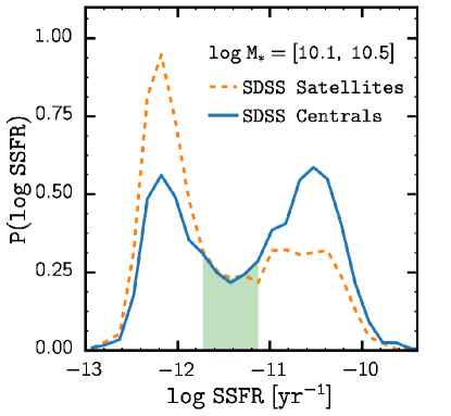
Figure 10.— SSFR distributions of the central galaxies versus the satellite galaxies in the SDSS DR7 Group Catalog with stellar mass between $10^{10.1}$ and $10^{10.5}\mathrm{M}_{\odot}$. Both SSFR distributions have similar green valley heights (green shaded region). Since central galaxies have significantly longer quenching timescales, satellite galaxies have a higher rate of transitioning from star-forming to quenching than central galaxies.

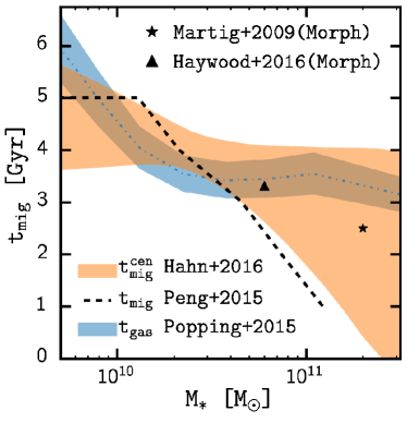
Figure 11.— Comparison of the central galaxy quenching migration time estimate we infer, ($t_{\mathrm{mig}}^{\mathrm{cen}}$; orange) with quenching time estimates for gas depletion absent accretion (strangulation) and morphological quenching. The width represents the 68 % confidence region propagated from the posterior distributions of the $\tau_{\mathrm{Q}}^{\mathrm{cen}}$ parameters. For strangulation, we include the gas depletion time at $z=0.2$ derived from the star formation efficiency estimates in Popping et al. (2015) (blue dash-dotted). The surrounding blue shaded region plots the range of gas depletion times at $z=0.15$ (longer) to $0.25$ (shorter). We also include the quenching migration time inferred from the Peng et al. (2015) gas regulation model (dashed). For morphological quenching we plot the quenching times taken from the star formation histories of the simulated galaxy in Martig et al. (2009) (star). We also include the quenching times of the Milky Way in Haywood et al. (2016) (triangle). The quenching timescale of strangulation exhibit a similar stellar mass dependence and is generally consistent with our central quenching timescales. Although its feasibility for a wider galaxy population is unexplored, the quenching timescale from morphological quenching is in good agreement with our timescale.

6.2. Quenching Star Formation in Central Galaxies

Numerous physical processes have been proposed in the literature to explain the quenching of star formation. Observations, however, have yet to identify the primary driver of quenching or consistently narrowing down proposed mechanisms. The quenching timescale we derive for central galaxies provides a key constraint for any of the proposed mechanisms. Only processes that agree with our central galaxy quenching timescales, can be the main driver for quenching star formation in central galaxies.

Merger driven quenching has often been proposed as a driving mechanism of star formation quenching (Springel et al. 2005; Hopkins et al. 2006, 2008a, 2008b). In this proposed mechanism, quenching is typically driven by gas-rich galaxy mergers which induce starburst and rapid black hole growth. Cosmological hydrodynamics simulations that examine mergers, however, conclude that quenching from mergers alone cannot produce a realistic red sequence (Gabor et al. 2010, 2011. Gabor et al. (2011) used an on-the-fly prescription to identify mergers and halos in order to test different prescriptions for quenching star formation. In addition to failing to produce a realistic red sequence, they find that mergers cannot sustain quiescence due to gas accretion from the inter-galactic medium, which refuels star formation after $1-2\;\mathrm{Gyr}$. The major mergers examined in the four high resolution zoom in cosmological hydrodynamic simulation of Sparre & Springel (2016) also fail to sustain quiescence after $1-2\;\mathrm{Gyr}$ (Sparre et al. in prep.).

AGN feedback has also been proposed as a quenching mechanism (Kauffmann & Haehnelt 2000; Croton et al. 2006; Hopkins et al. 2008a; van de Voort et al. 2011), sometimes in conjunction with mergers as a way to sustain quiescence or on its own. The feedback of the AGN deposit sufficient energy, which subsequently prevents additional gas from cooling. A number of more recent works have, however, cast doubt on the role of the AGN in quenching. Mendel et al. (2013), identified quenched galaxies, with selection criteria analogous to the selection of post-starburst galaxies, in the SDSS DR7 sample and found no excess of optical AGN in them, suggesting that AGN do not have defining role in quenching. Gabor & Bournaud (2014) further argue against AGN quenching by examining gas-rich, isolated disk galaxies in a suite of high resolution simulations where they find that the AGN outflows have little impact on the gas reservoir in the galaxy disk and furthermore fail to prevent gas inflow from the intergalactic medium. Yesuf et al. (2014) examined post-starburst galaxies transitioning from the blue cloud to the red sequence to find a significant time delay between the AGN activity and starburst phase, which suggests that AGN do not play a primary role in triggering quenching. AGN may yet be responsible for quenching in conjunction with other mechanisms or have a role in sustaining quiescence.

Besides mergers and AGN driven processes, another class of proposed mechanisms involves some process(es) that restrict the inflow of cold gas – strangulation. With little inflow of cold gas, the galaxy quenches as it depletes its cold gas reservoir. One mechanism that has been proposed to prevent cold gas accretion is loosely referred to as “halo quenching”. A hot gaseous coronae, which form in halos with masses above $\sim 10^{12}\mathrm{M}_{\odot}$ via virial shocks, starves galaxies of cold gas for star formation (Birnboim & Dekel 2003; Kereš et al. 2005; Cattaneo et al. 2006; Dekel & Birnboim 2006; Birnboim et al. 2007; Gabor & Davé 2012, 2015). For these sorts of mechanisms, the quenching timescale is linked to the time it takes for the galaxy to deplete its cold gas reservoir – the gas depletion timescale.

In principle, the gas depletion time can be estimated from measurements of the total gas mass or gas fraction. In Popping et al. (2015), for instance, they derive “star formation efficiency” (SFE; inverse of the gas depletion time) by dividing the SFR of the SFMS by the total galaxy gas mass that they infer from their semi-empirical model. These sorts of gas depletion time estimates, however, have significant redshift dependence because the gas fraction of galaxies do not evolve significantly over $z<1$ (Stewart et al. 2009; Santini et al. 2014; Popping et al. 2015).

Nevertheless, in Figure 11 we estimate the central quenching migration time ($t_{\mathrm{mig}}^{\mathrm{cen}}$; orange) – the time it takes central galaxies to migrate from the SFMS to quiescent estimated from our $\tau_{\mathrm{Q}}^{\mathrm{cen}}$ – to the gas depletion times derived from the Popping et al. (2015) SFEs (blue). For $t_{\mathrm{mig}}^{\mathrm{cen}}$, we compute the time it takes a quenching galaxy to transition from the SFMS to the quiescent peak of the SFR distribution at $z=0.2$. We compute $t_{\mathrm{mig}}^{\mathrm{cen}}$ at $z=0.2$ because this is approximately when the $z\approx 0$ green valley galaxies would have started quenching. For the gas depletion time, we invert the SFE at $z=0.2$, interpolated between the $z=0.$ and $z=0.5$ Popping et al. (2015) SFEs (blue dot-dashed). The surrounding blue shaded region marks the range of gas depletion times from $z=0.15$ (longer) to $0.25$ (shorter) to illustrate the significant redshift dependence. We also note that over the redshift range $z=0.5$ to $0.$, at $\mathcal{M}=10^{10}\mathrm{M}_{\odot}$, the Popping et al. (2015) gas depletion time varies from $\sim 2.5$ to $7\;\mathrm{Gyrs}$. The $t_{\mathrm{mig}}^{\mathrm{cen}}$ and gas depletion time in Figure 11 are generally in agreement with each other and exhibit similar mass dependence.

Beyond the estimates of gas depletion times from gas mass, recently Peng et al. (2015), using a gas regulation model (e.g. Lilly et al. 2013; Peng & Maiolino 2014), explored the impact that different quenching mechanisms have on the stellar metallicity of local galaxies from the SDSS DR7 sample. To reproduce the stellar metallicity difference between quiescent and star forming galaxies in their galaxy sample, they conclude that the primary mechanism for quenching is gas depletion absent accretion and it a typical quenching migration time of $t_{\mathrm{mig}}\sim 4\;\mathrm{Gyr}$ for $\mathcal{M}<10^{11}\mathrm{M}_{\odot}$. We infer the quenching migration time from Figure 2 of Peng et al. (2015) and include it in Figure 11 (dashed). The Peng et al. (2015) migration time exhibits a similar mass dependence as our central quenching migration time. Furthermore, although slightly shorter at $\mathcal{M}>5\times 10^{10}\mathrm{M}_{\odot}$, the migration time is broadly consistent with our central quenching migration time.

Overall, our $t_{\mathrm{mig}}^{\mathrm{cen}}$ is consistent with the migration time estimates of gas depletion mechanisms. In other words, our central galaxy quenching timescale is consistent with the timescales predicted by gas depletion absent accretion. One currently favored model for halting cold gas accretion – halo quenching – quenches galaxies that inhabit host halos with masses greater than some threshold $\sim 10^{12}\mathrm{M}_{\odot}$. Based on SHAM, this halo mass threshold corresponds to stellar masses of $\sim 10^{10.25}\mathrm{M}_{\odot}$. Yet, a significant fraction of the SDSS central galaxy population with stellar masses $<10^{10.25}\mathrm{M}_{\odot}$ are quiescent. While, scatter in the halo mass threshold and the stellar mass to halo mass relation, combined, may help resolve this tension, halo quenching, faces a number of other challenges. For instance, the predictions of halo quenching models are difficult to reconcile with the observed scatter in the stellar mass to halo mass relation (Tinker 2016). Furthermore, models that rely only on such ‘halo quenching’ still must account for the hot gas in the inner region of the halo, which, because of its high density, often has short cooling times of just $1-2~{}\mathrm{Gyr}$. Of course, the challenges of halo quenching does not rule out quenching from gas depletion absent accretion since other mechanisms may also prevent cold gas from accreting onto the central galaxy

Finally, morphological quenching has also been proposed as a mechanism responsible for quenching star formation. In the mechanism proposed by Martig et al. (2009), for instance, star formation in galactic disks are quenched once the galactic disks become dominated by a stellar bulge. This stabilizes the disk from fragmenting into bound, star forming clumps. In a cosmological zoom-in simulation of a $\sim 2\times 10^{11}\mathrm{M}_{\odot}$ galaxy selected to examine such a mechanism, Martig et al. (2009) finds that the galaxy quenches its star formation from $\sim 10~{}\mathrm{M}_{\odot}\mathrm{yr}^{-1}$ to $\sim 1.5~{}\mathrm{M}_{\odot}\mathrm{yr}^{-1}$ in $\sim 2.5\;\mathrm{Gyr}$ during the morphological quenching phase. A $\mathcal{M}\sim 2\times 10^{11}\mathrm{M}_{\odot}$ galaxy with $\hat{t}_{\mathrm{Q}}\sim 2.5\;\mathrm{Gyr}$ (star; Figure 11) is in good agreement with $\hat{t}_{\mathrm{Q}}^{\mathrm{cen}}$. Despite this agreement, morphological quenching faces a number of challenges. There is little evidence from modern cosmological hydrodynamic simulations that suggest that morphological quenching can drive anything beyond short timescale fluctuations in gas fueling and SFR. Furthermore, proposed morphological quenching mechanisms face the “cooling flow problem” where they fail to prevent gas cooling onto a galaxy. Without addressing this issue, proposed morphological quenching mechanisms cannot maintain quiescence.

Our own Milky Way galaxy, as Haywood et al. (2016) finds, after forming its bar undergoes quenching. In the star formation history of the Milky Way that Haywood et al. (2016) recovers, the SFR of the Milky Way decreases by an order of magnitude over the span of roughly $1.5\;\mathrm{Gyr}$. Converting to $\hat{t}_{\mathrm{Q}}$ in a similar fashion as our $\hat{t}_{\mathrm{Q}}^{\mathrm{cen}}$ estimates and assuming a Milky Way stellar mass of $\sim 6\times 10^{10}\mathrm{M}_{\odot}$ (Licquia & Newman 2015; Haywood et al. 2016), we find remarkable agreement with our $\hat{t}_{\mathrm{Q}}^{\mathrm{cen}}$ (Figure 11). Motivated by the contemporaneous formation of the bar with quenching, Haywood et al. (2016) suggest a bar driven (morphological) quenching mechanism that inhibits gas accretion through high level turbulence supported pressure that is generated from the shearing of the gaseous disk. Although, this proposal may resolve the cooling-flow problem, their arguments for the mechanism are qualitative and thus require more detailed investigation. Admittedly, however, this particular comparison is hastily made since quenching event occurs beyond the redshift probed by our simulation at $1<z<2$. Furthermore, after dramatic quenching episode, based on the star formation history that Haywood et al. (2016) recovers, the Milky Way resumes star formation at a much lower level.

The central quenching timescale we infer from our analysis provides key insight into the physical processes responsible for quenching star formation. It offers a means of assessing the feasibility of numerous quenching mechanisms, which operate on distinct timescale. Based on the latest models and simulations, merger driven quenching has fallen out of favor and AGN alone seem insufficient in triggering quenching. Mechanisms that halt cold gas accretion, such as halo quenching, predict quenching times generally consistent with our estimates from the central quenching timescale we derive. However, it fails to explain the significant low mass quiescent population of central galaxies. Morphological quenching, with its agreement in quenching time, may be a key physical mechanism in quenching star formation. However, more evidence is required that it can address the cooling flow problem and maintain quiescence. Furthermore, its role in the overall quenching of galaxy populations – not just single simulated galaxies – still remains to be explored.

7. Summary

Understanding the physical mechanisms responsible for quenching star formation in galaxies has been a long standing challenge for hierarchical galaxy formation models. Following the success of Wetzel et al. (2013) in constraining the quenching timescales of satellite galaxies, in this work, we focus on star formation quenching in central galaxies with a similar approach. Using a high resolution $N$-body simulation in conjunction with observations of the SMF, SFMS, and quiescent fraction at $z<1$, we construct a model that statistically tracks the star formation histories of central galaxies. The free parameters of our model dictate the height of the green valley at the initial redshift, the correction to the quenching probability, and most importantly, the quenching timescale of central galaxies,

Using ABC-PMC with our model, we infer parameter constraints that best reproduce the observations of the central galaxy SSFR distribution from the SDSS DR7 Group Catalog and the central galaxy quiescent fraction evolution. From the parameter constraints of our model, we find the following results:

1. The quenching timescale of central galaxies exhibit a significant mass dependence: more massive central galaxies have shorter quenching timescales. Over the stellar mass range $\mathcal{M}=10^{9.5}-10^{11.5}\mathrm{M}_{\odot}$, $\tau_{\mathrm{Q}}^{\mathrm{cen}}\sim 1.2-0.5\;\mathrm{Gyr}$. Based on these timescales, central galaxies take roughly $2$ to $5$ Gyrs to traverse the green valley.

2. The quenching timescale of central galaxies is significantly longer than the quenching timescale of satellite galaxies. This result is robust for extreme prescriptions of the SMF evolution in our simulation and even for different parameterizations of the central quiescent fraction.

3. The difference in quenching timescales of satellite and centrals suggest that different physical mechanisms are primary drivers of star formation quenching in satellites versus centrals. Satellite galaxies experience external “environment quenching” while central galaxies experience internal “self quenching”.

4. We compare the central quenching timescales we infer to the gas depletion timescales predicted by quenching through strangulation and find broad agreement. We also find good agreement with morphological quenching; however, its feasibility in maintaining quiescent and for a wider galaxy population remains to be explored.

Ultimately, the central galaxy quenching timescale we obtain in our analysis provides a crucial constraint for any proposed mechanism for star formation quenching.

One key component of our simulation is the use of SHAM to track evolution of stellar masses of central galaxies. As mentioned above, the central galaxy quenching timescale results we obtain remain unchanged if we use stellar mass growth from integrated SFR. However, the use of SHAM stellar masses neglects the connection between stellar mass growth and star formation history. To incorporate integrated SFR galaxy stellar mass growth in our simulation, however, a better understanding of the detailed relationship among stellar mass growth, host halo growth, and the observed stellar mass to halo mass relation is required. We will explore this in future work.

References

- Abazajian et al. (2009) Abazajian, K. N., Adelman-McCarthy, J. K., Agüeros, M. A., et al. 2009, ApJS, 182, 543
- Akeret et al. (2015) Akeret, J., Refregier, A., Amara, A., Seehars, S., & Hasner, C. 2015, Journal of Cosmology and Astroparticle Physics, 8, 043
- Baldry et al. (2006) Baldry, I. K., Balogh, M. L., Bower, R. G., et al. 2006, MNRAS, 373, 469
- Balogh et al. (2000) Balogh, M. L., Navarro, J. F., & Morris, S. L. 2000, ApJ, 540, 113
- Behroozi et al. (2013) Behroozi, P. S., Wechsler, R. H., & Conroy, C. 2013, ApJ, 770, 57
- Bekki (2009) Bekki, K. 2009, MNRAS, 399, 2221
- Birnboim & Dekel (2003) Birnboim, Y., & Dekel, A. 2003, MNRAS, 345, 349
- Birnboim et al. (2007) Birnboim, Y., Dekel, A., & Neistein, E. 2007, MNRAS, 380, 339
- Blanton (2006) Blanton, M. R. 2006, ApJ, 648, 268
- Blanton & Berlind (2007) Blanton, M. R., & Berlind, A. A. 2007, ApJ, 664, 791
- Blanton & Moustakas (2009) Blanton, M. R., & Moustakas, J. 2009, ARA&A, 47, 159
- Blanton & Roweis (2007) Blanton, M. R., & Roweis, S. 2007, AJ, 133, 734
- Blanton et al. (2003) Blanton, M. R., Hogg, D. W., Bahcall, N. A., et al. 2003, ApJ, 594, 186
- Blanton et al. (2005) Blanton, M. R., Schlegel, D. J., Strauss, M. A., et al. 2005, AJ, 129, 2562
- Borch et al. (2006) Borch, A., Meisenheimer, K., Bell, E. F., et al. 2006, A&A, 453, 869
- Brinchmann et al. (2004) Brinchmann, J., Charlot, S., White, S. D. M., et al. 2004, MNRAS, 351, 1151
- Bundy et al. (2006) Bundy, K., Ellis, R. S., Conselice, C. J., et al. 2006, ApJ, 651, 120
- Cameron & Pettitt (2012) Cameron, E., & Pettitt, A. N. 2012, MNRAS, 425, 44
- Campbell et al. (2015) Campbell, D., van den Bosch, F. C., Hearin, A., et al. 2015, MNRAS, 452, 444
- Cattaneo et al. (2006) Cattaneo, A., Dekel, A., Devriendt, J., Guiderdoni, B., & Blaizot, J. 2006, MNRAS, 370, 1651
- Chabrier (2003) Chabrier, G. 2003, PASP, 115, 763
- Coil et al. (2011) Coil, A. L., Blanton, M. R., Burles, S. M., et al. 2011, ApJ, 741, 8
- Cole et al. (2000) Cole, S., Lacey, C. G., Baugh, C. M., & Frenk, C. S. 2000, MNRAS, 319, 168
- Conroy et al. (2006) Conroy, C., Wechsler, R. H., & Kravtsov, A. V. 2006, ApJ, 647, 201
- Cool et al. (2013) Cool, R. J., Moustakas, J., Blanton, M. R., et al. 2013, ApJ, 767, 118
- Cooper et al. (2007) Cooper, M. C., Newman, J. A., Coil, A. L., et al. 2007, MNRAS, 376, 1445
- Cooper et al. (2010) Cooper, M. C., Coil, A. L., Gerke, B. F., et al. 2010, MNRAS, 409, 337
- Croton et al. (2006) Croton, D. J., Springel, V., White, S. D. M., et al. 2006, MNRAS, 365, 11
- Daddi et al. (2007) Daddi, E., Dickinson, M., Morrison, G., et al. 2007, ApJ, 670, 156
- Darvish et al. (2016) Darvish, B., Mobasher, B., Sobral, D., et al. 2016, ArXiv e-prints, arXiv:1605.03182
- Davis et al. (1985) Davis, M., Efstathiou, G., Frenk, C. S., & White, S. D. M. 1985, ApJ, 292, 371
- Dekel & Birnboim (2006) Dekel, A., & Birnboim, Y. 2006, MNRAS, 368, 2
- Di Matteo et al. (2005) Di Matteo, T., Springel, V., & Hernquist, L. 2005, Nature, 433, 604
- Dressler (1980) Dressler, A. 1980, ApJ, 236, 351
- Drory et al. (2009) Drory, N., Bundy, K., Leauthaud, A., et al. 2009, ApJ, 707, 1595
- Elbaz et al. (2007) Elbaz, D., Daddi, E., Le Borgne, D., et al. 2007, A&A, 468, 33
- Gabor & Bournaud (2014) Gabor, J. M., & Bournaud, F. 2014, MNRAS, 441, 1615
- Gabor & Davé (2012) Gabor, J. M., & Davé, R. 2012, MNRAS, 427, 1816
- Gabor & Davé (2015) —. 2015, MNRAS, 447, 374
- Gabor et al. (2010) Gabor, J. M., Davé, R., Finlator, K., & Oppenheimer, B. D. 2010, MNRAS, 407, 749
- Gabor et al. (2011) Gabor, J. M., Davé, R., Oppenheimer, B. D., & Finlator, K. 2011, MNRAS, 417, 2676
- Geha et al. (2012) Geha, M., Blanton, M. R., Yan, R., & Tinker, J. L. 2012, ApJ, 757, 85
- Gu et al. (2016) Gu, M., Conroy, C., & Behroozi, P. 2016, ArXiv e-prints, arXiv:1602.01099
- Gunn & Gott (1972) Gunn, J. E., & Gott, III, J. R. 1972, ApJ, 176, 1
- Hahn et al. (2016) Hahn, C., Vakili, M., Walsh, K., et al. 2016, ArXiv e-prints, arXiv:1607.01782
- Hahn et al. (2015) Hahn, C., Blanton, M. R., Moustakas, J., et al. 2015, ApJ, 806, 162
- Haywood et al. (2016) Haywood, M., Lehnert, M. D., Di Matteo, P., et al. 2016, A&A, 589, A66
- Hermit et al. (1996) Hermit, S., Santiago, B. X., Lahav, O., et al. 1996, MNRAS, 283, 709
- Hopkins & Beacom (2006) Hopkins, A. M., & Beacom, J. F. 2006, ApJ, 651, 142
- Hopkins et al. (2008a) Hopkins, P. F., Cox, T. J., Kereš, D., & Hernquist, L. 2008a, ApJS, 175, 390
- Hopkins et al. (2006) Hopkins, P. F., Hernquist, L., Cox, T. J., et al. 2006, ApJS, 163, 1
- Hopkins et al. (2008b) Hopkins, P. F., Hernquist, L., Cox, T. J., & Kereš, D. 2008b, ApJS, 175, 356
- Hubble (1936) Hubble, E. P. 1936, The Realm of the Nebulae (New Haven: Yale University Press)
- Ilbert et al. (2013) Ilbert, O., McCracken, H. J., Le Fèvre, O., et al. 2013, A&A, 556, A55
- Iovino et al. (2010) Iovino, A., Cucciati, O., Scodeggio, M., et al. 2010, A&A, 509, A40
- Ishida et al. (2015) Ishida, E. E. O., Vitenti, S. D. P., Penna-Lima, M., et al. 2015, Astronomy and Computing, 13, 1
- Karim et al. (2011) Karim, A., Schinnerer, E., Martínez-Sansigre, A., et al. 2011, ApJ, 730, 61
- Kauffmann & Haehnelt (2000) Kauffmann, G., & Haehnelt, M. 2000, MNRAS, 311, 576
- Kauffmann et al. (2003) Kauffmann, G., Heckman, T. M., White, S. D. M., et al. 2003, MNRAS, 341, 33
- Kereš et al. (2005) Kereš, D., Katz, N., Weinberg, D. H., & Davé, R. 2005, MNRAS, 363, 2
- Kovač et al. (2014) Kovač, K., Lilly, S. J., Knobel, C., et al. 2014, MNRAS, 438, 717
- Larson et al. (1980) Larson, R. B., Tinsley, B. M., & Caldwell, C. N. 1980, ApJ, 237, 692
- Leauthaud et al. (2012) Leauthaud, A., Tinker, J., Bundy, K., et al. 2012, ApJ, 744, 159
- Lee et al. (2015) Lee, N., Sanders, D. B., Casey, C. M., et al. 2015, ApJ, 801, 80
- Leja et al. (2013) Leja, J., van Dokkum, P., & Franx, M. 2013, ApJ, 766, 33
- Li & White (2009) Li, C., & White, S. D. M. 2009, MNRAS, 398, 2177
- Licquia & Newman (2015) Licquia, T. C., & Newman, J. A. 2015, ApJ, 806, 96
- Lilly et al. (2013) Lilly, S. J., Carollo, C. M., Pipino, A., Renzini, A., & Peng, Y. 2013, ApJ, 772, 119
- Lin & Kilbinger (2015) Lin, C.-A., & Kilbinger, M. 2015, A&A, 583, A70
- Lin et al. (2016) Lin, C.-A., Kilbinger, M., & Pires, S. 2016, ArXiv e-prints, arXiv:1603.06773
- Madau & Dickinson (2014) Madau, P., & Dickinson, M. 2014, ARA&A, 52, 415
- Marchesini et al. (2009) Marchesini, D., van Dokkum, P. G., Förster Schreiber, N. M., et al. 2009, ApJ, 701, 1765
- Martig et al. (2009) Martig, M., Bournaud, F., Teyssier, R., & Dekel, A. 2009, ApJ, 707, 250
- Mendel et al. (2013) Mendel, J. T., Simard, L., Ellison, S. L., & Patton, D. R. 2013, MNRAS, 429, 2212
- Moore et al. (1998) Moore, B., Lake, G., & Katz, N. 1998, ApJ, 495, 139
- More et al. (2009) More, S., van den Bosch, F. C., Cacciato, M., et al. 2009, MNRAS, 392, 801
- Moustakas et al. (2013) Moustakas, J., Coil, A. L., Aird, J., et al. 2013, ApJ, 767, 50
- Muldrew et al. (2012) Muldrew, S. I., Croton, D. J., Skibba, R. A., et al. 2012, MNRAS, 419, 2670
- Muzzin et al. (2013) Muzzin, A., Marchesini, D., Stefanon, M., et al. 2013, ApJ, 777, 18
- Noeske et al. (2007) Noeske, K. G., Weiner, B. J., Faber, S. M., et al. 2007, ApJ, 660, L43
- Oemler (1974) Oemler, Jr., A. 1974, ApJ, 194, 1
- Oliver et al. (2010) Oliver, S., Frost, M., Farrah, D., et al. 2010, MNRAS, 405, 2279
- Peng et al. (2015) Peng, Y., Maiolino, R., & Cochrane, R. 2015, Nature, 521, 192
- Peng & Maiolino (2014) Peng, Y.-j., & Maiolino, R. 2014, MNRAS, 443, 3643
- Peng et al. (2010) Peng, Y.-j., Lilly, S. J., Kovač, K., et al. 2010, ApJ, 721, 193
- Popping et al. (2015) Popping, G., Behroozi, P. S., & Peeples, M. S. 2015, MNRAS, 449, 477
- Salim et al. (2007) Salim, S., Rich, R. M., Charlot, S., et al. 2007, ApJS, 173, 267
- Santini et al. (2014) Santini, P., Maiolino, R., Magnelli, B., et al. 2014, A&A, 562, A30
- Schawinski et al. (2014) Schawinski, K., Urry, C. M., Simmons, B. D., et al. 2014, MNRAS, 440, 889
- Scoville et al. (2007) Scoville, N., Aussel, H., Brusa, M., et al. 2007, ApJS, 172, 1
- Smethurst et al. (2015) Smethurst, R. J., Lintott, C. J., Simmons, B. D., et al. 2015, MNRAS, 450, 435
- Sparre & Springel (2016) Sparre, M., & Springel, V. 2016, ArXiv e-prints, arXiv:1604.08205
- Springel et al. (2005) Springel, V., Di Matteo, T., & Hernquist, L. 2005, MNRAS, 361, 776
- Stewart et al. (2009) Stewart, K. R., Bullock, J. S., Wechsler, R. H., & Maller, A. H. 2009, ApJ, 702, 307
- Tinker et al. (2011) Tinker, J., Wetzel, A., & Conroy, C. 2011, ArXiv e-prints, arXiv:1107.5046 [astro-ph.CO]
- Tinker et al. (2016) Tinker, J., Wetzel, A., Conroy, C., & Mao, Y.-Y. 2016, ArXiv e-prints, arXiv:1609.03388
- Tinker (2016) Tinker, J. L. 2016, ArXiv e-prints, arXiv:1607.06099
- Tinker et al. (2013) Tinker, J. L., Leauthaud, A., Bundy, K., et al. 2013, ApJ, 778, 93
- Tinker & Wetzel (2010) Tinker, J. L., & Wetzel, A. R. 2010, ApJ, 719, 88
- Vale & Ostriker (2006) Vale, A., & Ostriker, J. P. 2006, MNRAS, 371, 1173
- van de Voort et al. (2011) van de Voort, F., Schaye, J., Booth, C. M., & Dalla Vecchia, C. 2011, MNRAS, 415, 2782
- Weinmann et al. (2006) Weinmann, S. M., van den Bosch, F. C., Yang, X., et al. 2006, MNRAS, 372, 1161
- Wetzel et al. (2012) Wetzel, A. R., Tinker, J. L., & Conroy, C. 2012, MNRAS, 424, 232
- Wetzel et al. (2013) Wetzel, A. R., Tinker, J. L., Conroy, C., & van den Bosch, F. C. 2013, MNRAS, 432, 336
- Wetzel et al. (2014) —. 2014, MNRAS, 439, 2687
- Weyant et al. (2013) Weyant, A., Schafer, C., & Wood-Vasey, W. M. 2013, ApJ, 764, 116
- Whitaker et al. (2012) Whitaker, K. E., van Dokkum, P. G., Brammer, G., & Franx, M. 2012, ApJ, 754, L29
- White (2002) White, M. 2002, ApJS, 143, 241
- White et al. (2010) White, M., Cohn, J. D., & Smit, R. 2010, MNRAS, 408, 1818
- Woo et al. (2016) Woo, J., Carollo, C. M., Faber, S. M., Dekel, A., & Tacchella, S. 2016, ArXiv e-prints, arXiv:1607.06091
- Wyder et al. (2007) Wyder, T. K., Martin, D. C., Schiminovich, D., et al. 2007, ApJS, 173, 293
- Yang et al. (2008) Yang, X., Mo, H. J., & van den Bosch, F. C. 2008, ApJ, 676, 248
- Yang et al. (2009) —. 2009, ApJ, 693, 830
- Yesuf et al. (2014) Yesuf, H. M., Faber, S. M., Trump, J. R., et al. 2014, ApJ, 792, 84
- York et al. (2000) York, D. G., Adelman, J., Anderson, Jr., J. E., et al. 2000, AJ, 120, 1579
- Zheng et al. (2007) Zheng, Z., Coil, A. L., & Zehavi, I. 2007, ApJ, 667, 760
- Zheng et al. (2005) Zheng, Z., Berlind, A. A., Weinberg, D. H., et al. 2005, ApJ, 633, 791
- Zu & Mandelbaum (2015) Zu, Y., & Mandelbaum, R. 2015, MNRAS, 454, 1161