DESPOT: Online POMDP Planning with Regularization

Abstract

The partially observable Markov decision process (POMDP) provides a principled general framework for planning under uncertainty, but solving POMDPs optimally is computationally intractable, due to the “curse of dimensionality” and the “curse of history”. To overcome these challenges, we introduce the Determinized Sparse Partially Observable Tree (DESPOT), a sparse approximation of the standard belief tree, for online planning under uncertainty. A DESPOT focuses online planning on a set of randomly sampled scenarios and compactly captures the “execution” of all policies under these scenarios. We show that the best policy obtained from a DESPOT is near-optimal, with a regret bound that depends on the representation size of the optimal policy. Leveraging this result, we give an anytime online planning algorithm, which searches a DESPOT for a policy that optimizes a regularized objective function. Regularization balances the estimated value of a policy under the sampled scenarios and the policy size, thus avoiding overfitting. The algorithm demonstrates strong experimental results, compared with some of the best online POMDP algorithms available. It has also been incorporated into an autonomous driving system for real-time vehicle control. The source code for the algorithm is available online.

1 Introduction

The partially observable Markov decision process (POMDP) (?) provides a principled general framework for planning in partially observable stochastic environments. It has a wide range of applications ranging from robot control (?), resource management (?) to medical diagnosis (?). However, solving POMDPs optimally is computationally intractable (?, ?). Even approximating the optimal solution is difficult (?). There has been substantial progress in the last decade (?, ?, ?, ?, ?, ?). However, it remains a challenge today to scale up POMDP planning and tackle POMDPs with very large state spaces and complex dynamics to achieve near real-time performance in practical applications (see, e.g., Figures 2 and 3).

Intuitively, POMDP planning faces two main difficulties. One is the “curse of dimensionality”. A large state space is a well-known difficulty for planning: the number of states grows exponentially with the number of state variables. Furthermore, in a partially observable environment, the agent must reason in the space of beliefs, which are probability distributions over the states. If one naively discretizes the belief space, the number of discrete beliefs then grows exponentially with the number of states. The second difficulty is the “curse of history”: the number of action-observation histories under consideration for POMDP planning grows exponentially with the planning horizon. Both curses result in exponential growth of computational complexity and major barriers to large-scale POMDP planning.

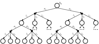
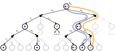
(a)	(b)

Figure 1: Online POMDP planning performs lookahead search on a tree. (a) A standard belief tree of height $D=2$. It contains all action-observation histories. Each belief tree node represents a belief. Each path represents an action-observation history. (b) A DESPOT (black), obtained under 2 sampled scenarios marked with blue and orange dots, is overlaid on the standard belief tree. A DESPOT contains only the histories under the sampled scenarios. Each DESPOT node represents a belief implicitly and contains a particle set that approximates the belief. The particle set consists of a subset of sampled scenarios.

This paper presents a new anytime online algorithm for POMDP planning. Online POMDP planning chooses one action at a time and interleaves planning and plan execution (?). At each time step, the agent performs lookahead search on a belief tree rooted at the current belief (Figure 1a) and executes immediately the best action found. To attack the two curses, our algorithm exploits two basic ideas: sampling and anytime heuristic search, described below.

To speed up lookahead search, we introduce the Determinized Sparse Partially Observable Tree (DESPOT) as a sparse approximation to the standard belief tree. The construction of a DESPOT leverages a set of randomly sampled scenarios. Intuitively, a scenario is a sequence of random numbers that determinizes the execution of a policy under uncertainty and generates a unique trajectory of states and observations given an action sequence. A DESPOT encodes the execution of all policies under a fixed set of $K$ sampled scenarios (Figure 1b). It alleviates the “curse of dimensionality” by sampling states from a belief and alleviates the “curse of history” by sampling observations. A standard belief tree of height $0pt$ contains all possible action-observation histories and thus $\mathcal{O}(|A|^{0}pt|Z|^{0}pt)$ belief nodes, where $|A|$ is the number of actions and $|Z|$ is the number of observations. In contrast, a corresponding DESPOT contains only histories under the $K$ sampled scenarios and thus $\mathcal{O}(|A|^{0}ptK)$ belief nodes. A DESPOT is much sparser than a standard belief tree when $K$ is small but converges to the standard belief tree as $K$ grows.

To approximate the standard belief tree well, the number of scenarios, $K$, required by a DESPOT may be exponentially large in the worst case. The worst case, however, may be uncommon in practice. We give a competitive analysis that compares our computed policy against near optimal policies and show that $K\in\mathcal{O}(|\pi|\ln(|\pi||A||Z|))$ is sufficient to guarantee near-optimal performance for the lookahead search, when a POMDP admits a near-optimal policy $\pi$ with representation size $|\pi|$ (Theorem 3.2). Consequently, if a POMDP admits a compact near-optimal policy, it is sufficient to use a DESPOT much smaller than a standard belief tree, significantly speeding up the lookahead search. Our experimental results support this view in practice: $K$ as small as 500 can work well for some large POMDPs.

As a DESPOT is constructed from sampled scenarios, lookahead search may overfit the sampled scenarios and find a biased policy. To achieve the desired performance bound, our algorithm uses regularization, which balances the estimated value of a policy under the sampled scenarios and the size of the policy. Experimental results show that when overfitting occurs, regularization is helpful in practice.

To further improve the practical performance of lookahead search, we introduce an anytime heuristic algorithm to search a DESPOT. The algorithm constructs a DESPOT incrementally under the guidance of a heuristic. Whenever the maximum planning time is reached, it outputs the action with the best regularized value based on the partially constructed DESPOT, thus endowing the algorithm with the anytime characteristic. We show that if the search heuristic is admissible, our algorithm eventually finds the optimal action, given sufficient time. We further show that if the heuristic is not admissible, the performance of the algorithm degrades gracefully. Graceful degradation is important, as it allows practitioners to use their intuition to design good heuristics that are not necessarily admissible over the entire belief space.

Figure 2: DESPOT running in real time on an autonomous golf-cart among many pedestrians.

Experiments show that the anytime DESPOT algorithm is successful on very large POMDPs with up to $10^{56}$ states. The algorithm is also capable of handling complex dynamics. We implemented it on a robot vehicle for intention-aware autonomous driving among many pedestrians (Figure 2). It achieved real-time performance on this system (?). In addition, the DESPOT algorithm is a core component of our autonomous mine detection strategy that won the 2015 Humanitarian Robotics and Automation Technology Challenge (?) (Figure 3).

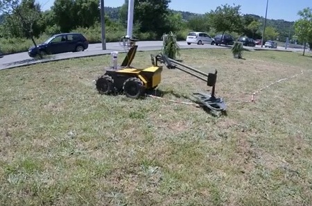
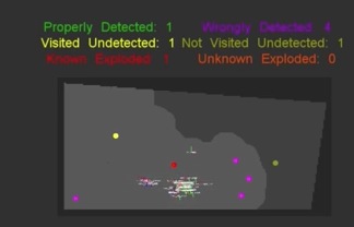
Figure 3: Robot mine detection in Humanitarian Robotics and Automation Technology Challenge 2015. Images used with permission of Lino Marques.

In the following, Section 2 reviews the background on POMDPs and related work. Section 3 defines the DESPOT formally and presents the theoretical analysis to motivate the use of a regularized objective function for lookahead search. Section 4 presents the anytime online POMDP algorithm, which searches a DESPOT for a near-optimal policy. Section 5 presents experiments that evaluate our algorithm and compare it with the state of the art. Section 6 discusses the strengths and the limitations of this work as well as opportunities for further work. We conclude with a summary in Section 7.

2 Background

We review the basics of online POMDP planning and related works in this section.

2.1 Online POMDP Planning

A POMDP models an agent acting in a partially observable stochastic environment. It can be specified formally as a tuple $(S,A,Z,T,O,R)$, where $S$ is a set of states, $A$ is a set of agent actions, and $Z$ is a set of observations. When the agent takes action $a\in A$ in state $s\in S$, it moves to a new state $s^{\prime}\in S$ with probability $T(s,a,s^{\prime})=p(s^{\prime}|s,a)$ and receives observation $z\in Z$ with probability $O(s^{\prime},a,z)=p(z|s^{\prime},a)$. It also receives a real-valued reward $R(s,a)$.

A POMDP agent does not know the true state, but receives observations that provide partial information on the state. The agent thus maintains a belief, represented as a probability distribution over $S$. It starts with an initial belief $b_{0}$. At time $t$, it updates the belief according to Bayes’ rule, by incorporating information from the action $a_{t}$ taken and the resulting observation $o_{t}$:

$$b_{t}(s^{\prime})=\eta{O(s^{\prime},a_{t},z_{t})}\sum_{s\in S}T(s,a_{t},s^{\prime})b_{t-1}(s),\vspace*{0pt}$$ (1)

where $\eta$ is a normalizing constant. The belief $b_{t}=\tau(b_{t-1},a_{t},z_{t})=\tau(\tau(b_{t-2},a_{t-1},z_{t-1}),a_{t},z_{t})=\cdots=\tau(\cdots\tau(\tau(b_{0},a_{1},b_{1}),a_{2},b_{2}),\ldots,a_{t},z_{t})$ is a sufficient statistic that contains all the information from the history of actions and observations $(a_{1},z_{1},a_{2},z_{2},\ldots,a_{t},z_{t})$.

A policy $\pi\colon\mathcal{B}\mapsto A$ is a mapping from the belief space $\mathcal{B}$ to the action space $A$. It prescribes an action $\pi(b)\in A$ at the belief $b\in\mathcal{B}$. For infinite-horizon POMDPs, the value of a policy $\pi$ at a belief $b$ is the expected total discounted reward that the agent receives by executing $\pi$:

$$V_{\pi}(b)=\mbox{$\textbf{{E}}$}\Bigl{(}\sum_{t=0}^{\infty}\gamma^{t}R\bigl{(}s_{t},\pi(b_{t})\bigr{)}\;\bigl{|}\;b_{0}=b\Bigr{)}.\vspace*{0pt}$$ (2)

The constant $\gamma\in[0,1)$ is a discount factor, which expresses preferences for immediate rewards over future ones.

In online POMDP planning, the agent starts with an initial belief. At each time step, it searches for an optimal action $a^{*}$ at the current belief $b$. The agent executes the action $a^{*}$ and receives a new observation $z$. It updates the belief using (1). The process then repeats.

To search for an optimal action $a^{*}$, one way is to construct a belief tree (Figure 1a), with the current belief $b_{0}$ as the initial belief at the root of the tree. The agent performs lookahead search on the tree for a policy $\pi$ that maximizes the value $V_{\pi}(b_{0})$ at $b_{0}$, and sets $a^{*}=\pi(b_{0})$. Each node of the tree represents a belief. To simplify the notation, we use the same notation $b$ to represent both the node and the associated belief. A node branches into $|A|$ action edges, and each action edge further branches into $|Z|$ observation edges. If a node and its child represent beliefs $b$ and $b^{\prime}$, respectively, then $b^{\prime}=\tau(b,a,z)$ for some $a\in A$ and $z\in Z$.

To obtain an approximately optimal policy, we may truncate the tree at a maximum depth 0ptand search for the optimal policy on the truncated tree. At each leaf node, we simulate a user-specified default policy to obtain a lower-bound estimate on its optimal value. A default policy, for example, can be a random policy or a heuristic. At each internal node $b$, we apply Bellman’s principle of optimality:

$$V^{*}(b)=\max_{a\in A}\Bigl{\{}\sum_{s\in S}{b(s)R(s,a)}+\gamma\sum_{z\in Z}p(z|b,a)V^{*}\bigl{(}\tau(b,a,z)\bigr{)}\Bigr{\}},\vspace*{0pt}$$ (3)

which computes the maximum value of action branches and the average value of observation branches weighted by the observation probabilities. We then perform a post-order traversal on the belief tree and use (3) to compute recursively the maximum value at each node and obtain the best action at the root node $b_{0}$ for execution.

Suppose that at each internal node $b$ in a belief tree, we retain only one action branch, which represents the chosen action at $b$, and remove all other branches. This transforms a belief tree into a policy tree. Each internal node $b$ of a policy tree has a single out-going action edge, which specifies the action at $b$. Each leaf node is associated with a default policy for execution at the node. Our DESPOT algorithm uses this policy tree representation. We define the size of such a policy as the number of internal policy tree nodes. A singleton policy tree thus has size $0$.

2.2 Related Work

There are two main approaches to POMDP planning: offline policy computation and online search. In offline planning, the agent computes beforehand a policy contingent upon all possible future outcomes and executes the computed policy based on the observations received. One main advantage of offline planning is fast policy execution, as the policy is precomputed. Early work on POMDP planning often takes the offline approach. See, e.g., the work of ? (?) and ? (?). Although offline planning algorithms have made major progress in recent years (?, ?, ?, ?), they still face significant difficulty in scaling up to very large POMDPs, as they must plan for all beliefs and future contingencies.

Online planning interleaves planning with plan execution. At each time step, it plans locally and chooses an optimal action for the current belief only, by performing lookahead search in the neighborhood of the current belief. It then executes the chosen action immediately. Planning for the current belief is computationally attractive. First, it is simpler to search for an optimal action at a single belief than to do so for all beliefs, as offline policy computation does. Second, it allows us to exploit local structure to reduce the search space size. One limitation of the online approach is the constraint on planning time. As it interleaves planning and plan execution, the plan must be ready for execution within short time in some applications.

A recent survey lists three main ideas for online planning via belief tree search (?): heuristic search, branch-and-bound pruning, and Monte Carlo sampling. Heuristic search employs a heuristic to guide the belief tree search (?, ?). This idea dates back to the early work of ? (?) . Branch-and-bound pruning maintains upper and lower bounds on the value at each belief tree node and use them to prune suboptimal subtrees and improve computational efficiency (?). This idea is also present in earlier work on offline POMDP planning (?). Monte Carlo sampling explores only a randomly sampled subset of observation branches at each node of the belief tree (?, ?, ?, ?). Our DESPOT algorithm contains all three ideas, but is most closely associated with Monte Carlo sampling. Below we examine some of the earlier Monte Carlo sampling algorithms and DESPOT’s connection with them.

The rollout algorithm (?) is an early example of Monte Carlo sampling for planning under uncertainty. It is originally designed for Markov decision processes (MDPs), but can be easily adapted to solve POMDPs as well. It estimates the value of a default heuristic policy by performing $K$ simulations and then chooses the best action by one-step lookahead search over the estimated values. Although a one-step lookahead policy improves over the default policy, it may be far from the optimum because of the very short, one-step search horizon.

Like the rollout algorithm, the hindsight optimization algorithm (HO) (?, ?) is intended for MDPs, but can be adapted for POMDPs. While both HO and DESPOT sample $K$ scenarios for planning, HO builds one tree with $\mathcal{O}(|A|^{0}pt)$ nodes for each scenario, independent of others, and thus $K$ trees in total. It searches each tree for an optimal plan and averages the values of these $K$ optimal plans to choose a best action. HO and related algorithms have been quite successful in recent international probabilistic planning competitions. However, HO plans for each scenario independently; it optimizes an upper bound on the value of a POMDP and not the true value itself. In contrast, DESPOT captures all $K$ scenarios in a single tree of $\mathcal{O}(|A|^{0}ptK)$ nodes and hedges against all $K$ scenarios simultaneously during the planning. It converges to the true optimal value of the POMDP as $K$ grows.

The work of ? (?) and that of ? (?) use sampled scenarios as well, but for offline POMDP policy computation. They provide uniform convergence bounds in terms of the complexity of the policy class under consideration, e.g., the Vapnik-Chervonenkis dimension. In comparison, DESPOT uses sampled scenarios for online instead of offline planning. Furthermore, our competitive analysis of DESPOT compares our computed policy against an optimal policy and produces a bound that depends on the size of the optimal policy. The bound benefits from the existence of a small near-optimal policy and naturally leads to a regularized objective function for online planning; in contrast, the algorithms by ? (?) and ? (?) do not exploit the existence of good small policies within the class of policies under consideration.

The sparse sampling (SS) algorithm (?) and the DESPOT algorithm both construct sparse approximations to a belief tree. SS samples a constant number $C$ of observation branches for each action. A sparse sampling tree contains $\mathcal{O}(|A|^{D}C^{D})$ nodes, while a DESPOT contains $\mathcal{O}(|A|^{D}K)$ nodes. Our analysis shows that $K$ can be much smaller than $C^{D}$ when a POMDP admits a small near-optimal policy (Theorem 3.2). In such cases, the DESPOT algorithm is computationally more efficient.

POMCP (?) performs Monte Carlo tree search (MCTS) on a belief tree. It combines optimistic action exploration and random observation sampling, and relies on the UCT algorithm (?) to trade off exploration and exploitation. POMCP is simple to implement and is one of the best in terms of practical performance on large POMDPs. However, it can be misguided by the upper confidence bound (UCB) heuristic of the UCT algorithm and be overly greedy. Although it converges to an optimal action in the limit, its worst-case running time is extremely poor: $\Omega(\overset{\scriptscriptstyle D-1}{\overbrace{\exp(\exp(\ldots\exp}}(1)\ldots)))$ (?).

Among the Monte Carlo sampling algorithms, one unique feature of DESPOT is the use of regularization to avoid overfitting to sampled scenarios: it balances the estimated performance value of a policy and the policy size during the online search, improving overall performance for suitable tasks.

Another important issue for online POMDP planning is belief representation. Most online POMDP algorithms, including the Monte Carlo sampling algorithms, explicitly represent the belief as a probability distribution over the state space. This severely limits their scalability on POMDPs with very large state spaces, because a single belief update can take time quadratic in the number of states. Notable exceptions are POMCP and DESPOT. Both represent the belief as a set of sampled states and do not perform belief update over the entire state space during the online search.

Online search and offline policy computation are complementary and can be combined, by using approximate or partial policies computed offline as the default policies at the leaves of the search tree for online planning (?, ?), or as macro-actions to shorten the search horizon (?).

This paper extends our earlier work (?). It provides an improved anytime online planning algorithm, an analysis of this algorithm, and new experimental results.

3 Determinized Sparse Partially Observable Trees

A DESPOT is a sparse approximation of a standard belief tree. While a standard belief tree captures the execution of all policies under all possible scenarios, a DESPOT captures the execution of all policies under a set of randomly sampled scenarios (Figure 1b). A DESPOT contains all the action branches, but only the observation branches encountered under the sampled scenarios.

We define DESPOT constructively by applying a deterministic simulative model to all possible action sequences under $K$ sampled scenarios. A scenario is an abstract simulation trajectory with some start state $s_{0}$. Formally, a scenario for a belief $b$ is an infinite random sequence ${\bm{\phi}}=(s_{0},\phi_{1},\phi_{2},\ldots)$, in which the start state $s_{0}$ is sampled according to $b$ and each $\phi_{i}$ is a real number sampled independently and uniformly from the range $[0,1]$. The deterministic simulative model is a function $g\colon S\times A\times\textrm{R}\mapsto S\times Z$, such that if a random number $\phi$ is distributed uniformly over $[0,1]$, then $(s^{\prime},z^{\prime})=g(s,a,\phi)$ is distributed according to $p(s^{\prime},z^{\prime}|s,a)=T(s,a,s^{\prime})O(s^{\prime},a,z^{\prime})$. When simulating this model for an action sequence $(a_{1},a_{2},\ldots)$ under a scenario $(s_{0},\phi_{1},\phi_{2},\ldots)$, we get a simulation trajectory $(s_{0},a_{1},s_{1},z_{1},a_{2},s_{2},z_{2},\ldots)$, where $(s_{t},z_{t})=g(s_{t-1},a_{t},\phi_{t})$ for $t=1,2,\ldots$ . The simulation trajectory traces out a path $(a_{1},z_{1},a_{2},z_{2},\ldots)$ from the root of the standard belief tree. We add all the nodes and edges on this path to the DESPOT $\mathcal{D}$ being constructed. Each node $b$ of $\mathcal{D}$ contains a set ${\bm{\Phi}}_{b}$ of all scenarios that it encounters. We insert the scenario $(s_{0},\phi_{0},\phi_{1},\ldots)$ into the set ${\bm{\Phi}}_{b_{0}}$ at the root $b_{0}$ and insert the scenario $(s_{t},\phi_{t+1},\phi_{t+2},\ldots)$ into the set ${\bm{\Phi}}_{b_{t}}$ at the belief node $b_{t}$ reached at the end of the subpath $(a_{1},z_{1},a_{2},z_{2},\ldots,a_{t},z_{t})$, for $t=1,2,\ldots$ . Repeating this process for every action sequence under every sampled scenario completes the construction of $\mathcal{D}$.

In summary, a DESPOT is a randomly sampled subtree of a standard belief tree. It is completely determined by the set of $K$ random sequences sampled a priori, hence the name Determinized Sparse Partially Observable Tree. Each DESPOT node $b$ represents a belief and contains a set ${\bm{\Phi}}_{b}$ of scenarios. The start states of the scenarios in ${\bm{\Phi}}_{b}$ form a particle set that represents $b$ approximately. While a standard belief tree of height 0pthas $\mathcal{O}(|A|^{0}pt|Z|^{0}pt)$ nodes, a corresponding DESPOT has $\mathcal{O}(|A|^{0}ptK)$ nodes for $|A|\geq 2$, because of reduced observation branching under the sampled scenarios.

It is possible to search for near-optimal policies using a DESPOT instead of a standard belief tree. The empirical value $\hat{V}_{\pi}(b)$ of a policy $\pi$ under the sampled scenarios encoded in a DESPOT is the average total discounted reward obtained by simulating the policy under each scenario. Formally, let $V_{\pi,{\bm{\phi}}}$ be the total discounted reward of the trajectory obtained by simulating $\pi$ under a scenario ${\bm{\phi}}\in{\bm{\Phi}}_{b}$ for some node $b$ in a DESPOT, then

$$\hat{V}_{\pi}(b)=\sum_{{\bm{\phi}}\in{\bm{\Phi}}_{b}}{V_{\pi,{\bm{\phi}}}\over|{\bm{\Phi}}_{b}|},\vspace*{0pt}$$

where $|{\bm{\Phi}}_{b}|$ is the number of scenarios in ${\bm{\Phi}}_{b}$. Since $\hat{V}_{\pi}(b)$ converges to $V_{\pi}(b)$ almost surely as $K\rightarrow\infty$, the problem of finding an optimal policy at $b$ can be approximated as that of doing so under the sampled scenarios. One concern, however, is overfitting: a policy optimized for finitely many sampled scenarios may not be optimal in general, as many scenarios are not sampled. To control overfitting, we regularize the empirical value of a policy by adding a term that penalizes large policy size. We now provide theoretical analysis to justify this approach.

Our first result bounds the error of estimating the values of all policies derived from DESPOTs of a given size. The result implies that a DESPOT constructed with a small number of scenarios is sufficient for approximate policy evaluation. The second result shows that by optimizing this bound, which is equivalent to maximizing a regularized value function, we obtain a policy that is competitive with the best small policy.

Formally, a DESPOT policy $\pi$ is a policy tree derived from a DESPOT $\mathcal{D}$: $\pi$ contains the same root as the DESPOT $\mathcal{D}$, but only one action branch at each internal node. To execute $\pi$, an agent starts at the root of $\pi$. At each time step, it takes the action specified by the action edge at the node. Upon receiving the resulting observation, it follows the corresponding observation edge to the next node. The agent may encounter an observation not present in $\pi$, as $\pi$ contains only the observation branches under the sampled scenarios. In this case, the agent follows a default policy from then on. Similarly, it follows the default policy when reaching a leaf node of $\pi$. Consider the set $\Pi_{b_{0},0pt,K}$, which contains all DESPOT policies derived from DESPOTs of height $0pt$, constructed with all possible $K$ sampled scenarios for a belief $b_{0}$. We now bound the error on the estimated value of an arbitrary DESPOT policy in $\Pi_{b_{0},0pt,K}$. To simplify the presentation, we assume without loss of generality that all rewards are non-negative and are bounded by $R_{\mathrm{max}}$. For models with bounded negative rewards, we can shift all rewards by a constant to make them non-negative. The shift does not affect the optimal policy.

Theorem 3.1.

For any given constants $\tau,\alpha\in(0,1)$, any belief $b_{0}$, and any positive integers $D$ and $K$, every DESPOT policy tree $\pi\in\Pi_{b_{0},0pt,K}$ satisfies

$$V_{\pi}(b_{0})\geq\frac{1-\alpha}{1+\alpha}\hat{V}_{\pi}(b_{0})-\frac{R_{\mathrm{max}}}{(1+\alpha)(1-\gamma)}\cdot\frac{\ln(4/\tau)+|\pi|\ln\bigl{(}KD|A||Z|\bigr{)}}{\alpha K}\vspace*{0pt}$$ (4)

with probability at least $1-\tau$, where $\hat{V}_{\pi}(b_{0})$ is the estimated value of $\pi$ under a set of $K$ scenarios randomly sampled according to $b_{0}$.

All proofs are presented in the appendix. Intuitively, the result says that all DESPOT policies in $\Pi_{b_{0},0pt,K}$ satisfy the bound given in (4), with high probability. The bound holds for any constant $\alpha\in(0,1)$, which is a parameter that can be tuned to tighten the bound. A smaller $\alpha$ value reduces the approximation error in the first term on the right-hand side of (4), but increases the additive error in the second term. The additive error depends on the size of $\pi$. It also grows logarithmically with $|A|$ and $|Z|$. The estimation thus scales well with large action and observation spaces. We can make this estimation error arbitrarily small by choosing a suitable number of sampled scenarios, $K$.

The next theorem states that we can obtain a near-optimal policy ${\hat{}\pi}$ by maximizing the RHS of (4), which accounts for both the estimated performance and the size of a policy.

Theorem 3.2.

Let $\pi$ be an arbitrary policy at a belief $b_{0}$. Let $\Pi_{\mathcal{D}}$ be the set of policies derived from a DESPOT $\mathcal{D}$ that has height 0ptand is constructed with $K$ scenarios sampled randomly according to $b_{0}$. For any given constants $\tau,\alpha\in(0,1)$, if

$$\small{\hat{}\pi}=\operatorname*{arg\,max}_{\pi^{\prime}\in\Pi_{\mathcal{D}}}\biggl{\{}\frac{1-\alpha}{1+\alpha}\hat{V}_{\pi^{\prime}}(b_{0})-\frac{R_{\max}}{(1+\alpha)(1-\gamma)}\cdot\frac{|\pi^{\prime}|\ln\bigl{(}KD|A||Z|\bigr{)}}{\alpha K}\biggr{\}},\vspace*{0pt}$$ (5)

then

with probability at least $1-\tau$.

Theorem 3.2 bounds the performance of $\hat{}\pi$, the policy maximizing (5) in the DESPOT, in terms of the performance of another policy $\pi$. Any policy can be used as the policy $\pi$ for comparison in the competitive analysis. Hence, the performance of $\hat{}\pi$ can be compared to the performance of an optimal policy. If the optimal policy has small representation size, the approximation error of $\hat{}\pi$ is correspondingly small. The performance of $\hat{}\pi$ is also robust. If the optimal policy has large size, but is well approximated by a small policy $\pi$ of size $|\pi|$, then we can obtain $\hat{}\pi$ with small approximation error, by choosing $K$ to be $\mathcal{O}(|\pi|\ln(|\pi||A||Z|))$. Since a DESPOT has size $\mathcal{O}(|A|^{0}ptK)$, the choice of $K$ allows us to trade off computation cost and approximation accuracy.

The objective function in (5) has the form

$$\hat{V}_{\pi}(b_{0})-\lambda|\pi|\vspace*{0pt}$$ (6)

for some $\lambda\geq 0$, similar to that of regularized utility functions in many machine learning algorithms. This motivates the regularized objective function for our online planning algorithm described in the next section.

4 Online Planning with DESPOTs

Following the standard online planning framework (Section 2.1), our algorithm iterates over two main steps: action selection and belief update. For belief update, we use a standard particle filtering method, sequential importance resampling (SIR) (?).

We now present two action selection methods. In Section 4.1, we describe a conceptually simple dynamic programming method that constructs a DESPOT fully before finding the optimal action. For very large POMDPs, constructing the DESPOT fully is not practical. In Sections 4.2 to 4.4, we describe an anytime DESPOT algorithm that performs anytime heuristic search. The anytime algorithm constructs a DESPOT incrementally under the guidance of a heuristic and scales up to very large POMDPs in practice. In Section 4.5, we show that the algorithm converges to an optimal policy when the heuristic is admissible and that the performance of the algorithm degrades gracefully even when the heuristic is not admissible.

4.1 Dynamic Programming

We construct a fixed DESPOT $\mathcal{D}$ with $K$ randomly sampled scenarios and want to derive from $\mathcal{D}$ a policy that maximizes the regularized empirical value (6) under the sampled scenarios:

$$\max_{\pi\in\Pi_{\mathcal{D}}}\Bigl{\{}\hat{V}_{\pi}(b_{0})-\lambda|\pi|\Bigr{\}},\vspace*{0pt}$$

where $b_{0}$ is the current belief, at the root of $\mathcal{D}$. Recall that a DESPOT policy is represented as a policy tree. For each node $b$ of $\pi$, we define the regularized weighted discounted utility (RWDU):

$$\nu_{\pi}(b)=\frac{|{\bm{\Phi}}_{b}|}{K}\gamma^{0pt(b)}\hat{V}_{\pi_{b}}(b)-\lambda|\pi_{b}|,$$ (7)

where $|{\bm{\Phi}}_{b}|$ is the number of scenarios passing through node $b$, $\gamma$ is the discount factor, $0pt(b)$ is the depth of $b$ in the policy tree $\pi$, $\pi_{b}$ is the subtree rooted at $b$, and $|\pi_{b}|$ is the size of $\pi_{b}$. The ratio ${|{\bm{\Phi}}_{b}|}/{K}$ is an empirical estimate of the probability of reaching $b$. Clearly, $\nu_{\pi}(b_{0})=\hat{V}_{\pi}(b_{0})-\lambda|\pi|$, which we want to optimize.

For every node $b$ of $\mathcal{D}$, define $\nu^{*}(b)$ as the maximum RWDU of $b$ over all policies in $\Pi_{\mathcal{D}}$. Assume that $\mathcal{D}$ has finite depth. We now present a dynamic programming procedure that computes $\nu^{*}(b_{0})$ recursively from bottom up. At a leaf node $b$ of $\mathcal{D}$, we simulate a default policy $\pi_{0}$ under the sampled scenarios. According to our definition in Section 2.1, $|\pi_{0}|=0$. Thus,

$$\nu^{*}(b)=\frac{|{\bm{\Phi}}_{b}|}{K}\gamma^{0pt(b)}\hat{V}_{\pi_{0}}(b).\vspace*{0pt}$$ (8)

At each internal node $b$, let $\tau(b,a,z)$ be the child of $b$ following the action branch $a$ and the observation branch $z$ at $b$. Then,

$$\nu^{*}(b) =\max\biggl{\{}\frac{|{\bm{\Phi}}_{b}|}{K}\gamma^{0pt(b)}\hat{V}_{\pi_{0}}(b),\;\max_{a\in A}\Bigr{\{}\rho(b,a)+\sum_{z\in Z_{b,a}}\nu^{*}(\tau(b,a,z))\Bigl{\}}\biggr{\}},$$ (9)

where

$$\rho(b,a) ={1\over K}\sum_{{\bm{\phi}}\in{\bm{\Phi}}_{b}}{\gamma^{0pt(b)}}R(s_{\bm{\phi}},a)-\lambda,$$

the state $s_{\bm{\phi}}$ is the start state of the scenario ${\bm{\phi}}$, and $Z_{b,a}$ is the set of observations following the action branch $a$ at the node $b$. The outer maximization in (9) chooses between executing the default policy or expanding the subtree at $b$. As the RWDU contains a regularization term, the latter is beneficial only if the subtree at $b$ is relatively small. This effectively prevents expanding a large subtree, when there are an insufficient number of sampled scenarios to estimate the value of a policy at $b$ accurately. The inner in (9) maximization chooses among the different actions available. When the algorithm terminates, the maximizer at the root $b_{0}$ of $\mathcal{D}$ gives the best action at $b_{0}$.

If $\mathcal{D}$ has unbounded depth, it is sufficient to truncate $\mathcal{D}$ to a depth of $\lceil{R_{\mathrm{max}}}/{\lambda(1-\gamma)}\rceil+1$ and run the above algorithm, provided that $\lambda>0$. The reason is that an optimal regularized policy $\hat{}\pi$ cannot include the truncated nodes of $\mathcal{D}$. Otherwise, $\hat{}\pi$ has size at least $\lceil{R_{\mathrm{max}}}/{\lambda(1-\gamma)}\rceil+1$ and thus RWDU $\nu_{\hat{}\pi}(b_{0})<0$. Since the default policy $\pi_{0}$ has RWDU $\nu_{\pi_{0}}(b_{0})\geq 0$, $\pi_{0}$ is then better than $\hat{}\pi$, a contradiction.

This dynamic programming algorithm runs in time linear in the number of nodes in $\mathcal{D}$. We first simulate the deterministic model to construct the tree, then do a bottom-up dynamic programming to initialize $\hat{V}_{\pi_{0}}(b)$, and finally compute $\nu^{*}(b)$ using Equation (9). Each step takes time linear in the number of nodes in $\mathcal{D}$ given previous steps are done, and thus the total running time is $\mathcal{O}(|A|^{0}ptK)$.

4.2 Anytime Heuristic Search

The bottom-up dynamic programming algorithm in the previous section constructs the full DESPOT $\mathcal{D}$ in advance. This is generally not practical because there are exponentially many nodes. To scale up, we now present an anytime forward search algorithm that avoids constructing the DESPOT fully in advance. It selects the action by incrementally constructing a DESPOT $\mathcal{D}$ rooted at the current belief $b_{0}$, using heuristic search (?, ?), and approximating the optimal RWDU $\nu^{*}(b_{0})$. We describe the main components of the algorithm below. The complete pseudocode is given in Appendix B.

To guide the heuristic search, we maintain a lower bound $\ell(b)$ and an upper bound $\mu(b)$ on the optimal RWDU at each node $b$ of $\mathcal{D}$, so that $\ell(b)\leq\nu^{*}(b)\leq\mu(b)$. To prune the search tree, we additionally maintain an upper bound $U(b)$ on the empirical value $\hat{V}^{*}(b)$ of the optimal regularized policy so that $U(b)\geq\hat{V}^{*}(b)$ and compute an initial lower bound $L_{0}(b)$ with $L_{0}(b)\leq\hat{V}^{*}(b)$. In particular, we use $L_{0}(b)=\hat{V}_{\pi_{0}}(b)$ for the default policy $\pi_{0}$ at $b$.

Algorithm 1 $\textsc{BuildDespot}({b}_{0})$

1:  Sample randomly a set ${\bm{\Phi}}_{{b}_{0}}$ of $K$ scenarios from the current belief ${b}_{0}$.

2:  Create a new DESPOT $\mathcal{D}$ with a single node ${b}_{0}$ as the root.

3:  Initialize $U({b}_{0}),L_{0}({b}_{0}),\mu({b}_{0}),\text{ and }\ell({b}_{0})$.

4:  $\epsilon({b}_{0})\leftarrow\mu({b}_{0})-\ell({b}_{0})$.

5:  while $\epsilon({b}_{0})>\epsilon_{0}$ and the total running time is less than $T_{\mathrm{max}}$ do

6:     $b\leftarrow\textsc{Explore}(\mathcal{D},{b}_{0})$.

7:     $\textsc{Backup}(\mathcal{D},b)$.

8:     $\epsilon({b}_{0})\leftarrow\mu({b}_{0})-\ell({b}_{0})$.

9:  return  $\ell$

Algorithm 1 provides a high-level sketch of the algorithm. We construct and search a DESPOT $\mathcal{D}$ incrementally, using $K$ sampled scenarios (line 1). Initially, $\mathcal{D}$ contains only a single root node with belief ${b}_{0}$ and the associated initial upper and lower bounds (lines 2–3). The algorithm makes a series of explorations to expand $\mathcal{D}$ and reduce the gap between the bounds $\mu(b_{0})$ and $\ell({b}_{0})$ at the root node ${b}_{0}$ of $\mathcal{D}$. Each exploration follows a heuristic and traverses a promising path from the root of $\mathcal{D}$ to add new nodes to $\mathcal{D}$ (line 6). Specifically, it keeps on choosing and expanding a promising leaf node and adds its child nodes into $\mathcal{D}$ until current leaf node is not heuristically promising. The algorithm then traces the path back to the root and performs backup on the upper and lower bounds at each node along the way, using Bellman’s principle (line 7). The explorations continue, until the gap between the bounds $\mu({b}_{0})$ and $\ell({b}_{0})$ reaches a target level $\epsilon_{0}\geq 0$ or the allocated online planning time runs out (line 5).

4.2.1 Forward Exploration

Algorithm 2 $\textsc{Explore}(\mathcal{D},b)$

1:  while $0pt(b)\leq D$, $E(b)>0$, and Prune($\mathcal{D}$, $b$) = FALSE do

2:     if $b$ is a leaf node in $\mathcal{D}$ then

3:        Expand $b$ one level deeper. Insert each new child $b^{\prime}$ of $b$ into $\mathcal{D}$. Initialize $U(b^{\prime})$, $L_{0}(b^{\prime})$, $\mu(b^{\prime})$, and $\ell(b^{\prime})$.

4:     $a^{*}\leftarrow\operatorname*{arg\,max}_{a\in A}{\mu(b,a)}$.

5:     $z^{*}\leftarrow\operatorname*{arg\,max}_{z\in Z_{b,a^{*}}}E(\tau(b,a^{*},z))$.

6:     $b\leftarrow\tau(b,a^{*},z^{*})$.

7:  if $0pt(b)>D$ then

8:     MakeDefault($b$).

9:  return  $b$.

Algorithm 3 MakeDefault($b$)

  $U(b)\leftarrow L_{0}(b)$.

  $\mu(b)\leftarrow\ell_{0}(b)$.

  $\ell(b)\leftarrow\ell_{0}(b)$.

Let $\epsilon(b)=\mu(b)-\ell(b)$ denote the gap between the upper and lower RWDU bounds at a node $b$. Each exploration aims to reduce the current gap $\epsilon(b_{0})$ at the root $b_{0}$ to $\xi\epsilon(b_{0})$ for some given constant $0<\xi<1$ (Algorithm 2). An exploration starts at the root $b_{0}$. At each node $b$ along the exploration path, we choose the action branch optimistically according to the upper bound $\mu(b)$:

$$a^{*}=\operatorname*{arg\,max}_{a\in A}\mu(b,a)=\operatorname*{arg\,max}_{a\in A}\Bigl{\{}\rho(b,a)+\sum_{z\in Z_{b,a}}\mu(b^{\prime})\Bigr{\}},\vspace*{0pt}$$ (10)

where $b^{\prime}=\tau(b,a,z)$ is the child of $b$ following the action branch $a$ and the observation branch $z$ at $b$. We then choose the observation branch $z$ that leads to a child node $b^{\prime}=\tau(b,a^{*},z)$ maximizing the excess uncertainty $E(b^{\prime})$ at $b^{\prime}$:

$$z^{*}=\operatorname*{arg\,max}_{z\in Z_{b,a^{*}}}E(b^{\prime})=\operatorname*{arg\,max}_{z\in Z_{b,a^{*}}}\Bigl{\{}\epsilon(b^{\prime})-\frac{|{\bm{\Phi}}_{b^{\prime}}|}{K}\cdot\xi\,\epsilon(b_{0})\Bigr{\}}.\vspace*{0pt}$$ (11)

Intuitively, the excess uncertainty $E(b^{\prime})$ measures the difference between the current gap at $b^{\prime}$ and the “expected” gap at $b^{\prime}$ if the target gap $\xi\,\epsilon(b_{0})$ at $b_{0}$ is satisfied. Our exploration strategy seeks to reduce the excess uncertainty in a greedy manner. See Lemma 4.1 in Section 4.5, the work of ? (?) and the work of ? (?) for justifications of this strategy.

If the exploration encounters a leaf node $b$, we expand $b$ by creating a child $b^{\prime}$ of $b$ for each action $a\in A$ and each observation encountered under a scenario ${\bm{\phi}}\in{\bm{\Phi}}_{b}$. For each new child $b^{\prime}$, we need to compute the initial bounds $\mu_{0}(b^{\prime})$, $\ell_{0}(b^{\prime})$, $U_{0}(b^{\prime})$, and $L_{0}(b^{\prime})$. The RWDU bounds $\mu_{0}(b^{\prime})$ and $\ell_{0}(b^{\prime})$ can be expressed in terms of the empirical value bounds $U_{0}(b^{\prime})$ and $L_{0}(b^{\prime})$, respectively. Applying the default policy $\pi_{0}$ at $b^{\prime}$ and using the definition of RWDU in (7), we have

$$\ell_{0}(b^{\prime})=\nu_{\pi_{0}}(b^{\prime})=\frac{|{\bm{\Phi}}_{b^{\prime}}|}{K}\gamma^{0pt(b^{\prime})}L_{0}(b^{\prime}),\vspace*{0pt}$$

as $|\pi_{0}|=0$. For the initial upper bound $\mu_{0}(b^{\prime})$, there are two cases. If the policy for maximizing the RWDU at $b^{\prime}$ is the default policy, then we can set $\mu_{0}(b^{\prime})=\ell_{0}(b^{\prime})$. Otherwise, the optimal policy has size at least $1$, and it follows from (7) that $\mu_{0}(b^{\prime})={|{\bm{\Phi}}_{b^{\prime}}|\over K}\gamma^{0pt(b^{\prime})}U_{0}(b^{\prime})-\lambda$ is an upper bound. So we have

$$\mu_{0}(b^{\prime}) =\max\Bigl{\{}\ell_{0}(b^{\prime}),\frac{|{\bm{\Phi}}_{b^{\prime}}|}{K}\gamma^{0pt(b^{\prime})}U_{0}(b^{\prime})-\lambda\Bigr{\}}.$$

There are various way to construct the initial empirical value bounds $U_{0}$ and $L_{0}$. We defer the discussion to Sections 4.3 and 4.4.

Note that a node at a depth more than $D$ executes the default policy, and the bounds are set accordingly using the MakeDefault procedure (Algorithm 3). We explain the termination conditions for exploration next.

4.2.2 Termination of Exploration and Pruning

We terminate the exploration at a node $b$ under three conditions (Algorithm 2, line 1). First, $0pt(b)>D$, i.e., the maximum tree height is exceeded. Second, $E(b)<0$, indicating that the expected gap at $b$ is reached and further exploration from $b$ onwards may be unprofitable. Finally, $b$ is blocked by an ancestor node $b^{\prime}$:

$$\frac{|{\bm{\Phi}}_{b^{\prime}}|}{K}\gamma^{0pt(b^{\prime})}(U(b^{\prime})-L_{0}(b^{\prime}))\leq\lambda\cdot\ell(b^{\prime},b),\vspace*{0pt}$$ (12)

where $\ell(b^{\prime},b)$ is the number of nodes on the path from $b^{\prime}$ to $b$. The intuition behind this last condition is that there is insufficient number of sampled scenarios at the ancestor node $b^{\prime}$. Further expanding $b$ and thus enlarging the policy subtree at $b^{\prime}$ may cause overfitting and reduce the regularized utility at $b^{\prime}$. We thus prune the search by applying the default policy at $b$ and setting the bounds accordingly by calling MakeDefault. More details are available in Lemma 4.2, which derives the condition (12) and proves that pruning the search does not compromise the optimality of the algorithm.

The pruning process continues backwards from $b$ towards the root of $\mathcal{D}$ (Algorithm 4). As the bounds are updated, new nodes may satisfy the condition for pruning and are pruned away.

Algorithm 4 Prune($\mathcal{D},b$)

1:  $\textsc{Blocked}\leftarrow\text{\small FALSE}$.

2:  for each node $x$ on the path from $b$ to the root of $\mathcal{D}$ do

3:     if $x$ is blocked by any ancestor node in $\mathcal{D}$ then

4:        MakeDefault($x$).

5:        Backup($\mathcal{D}$, $x$).

6:        $\textsc{Blocked}\leftarrow\text{\small TRUE}$.

7:     else

8:        break

9:  return  Blocked

4.2.3 Backup

When the exploration terminates, we trace the path back to the root and perform backup on the bounds at each node $b$ along the way, using Bellman’s principle (Algorithm 5):

$$\mu(b) =\max\Bigl{\{}\ell_{0}(b),\max_{a\in A}\Big{\{}\rho(b,a)+\sum_{z\in Z_{b,a}}\mu(b^{\prime})\Bigr{\}}\Bigr{\}},$$

$$\ell(b) =\max\Bigl{\{}\ell_{0}(b),\max_{a\in A}\Big{\{}\rho(b,a)+\sum_{z\in Z_{b,a}}\ell(b^{\prime})\Bigr{\}}\Bigr{\}},$$

$$U(b) =\max_{a\in A}\biggl{\{}\frac{1}{|{\bm{\Phi}}_{b}|}\sum_{{\bm{\phi}}\in{\bm{\Phi}}_{b}}R(s_{\bm{\phi}},a)+\gamma\sum_{z\in Z_{b,a}}\frac{|{\bm{\Phi}}_{b^{\prime}}|}{|{\bm{\Phi}}_{b}|}U(b^{\prime})\biggr{\}},$$

where $b^{\prime}$ is a child of $b$ with $b^{\prime}=\tau(b,a,z)$.

Algorithm 5 Backup($\mathcal{D},b$)

1:  for each node $x$ on the path from $b$ to the root of $\mathcal{D}$ do

2:     Perform backup on $\mu(x)$, $\ell(x)$, and $U(x)$.

4.2.4 Running Time

Suppose that the anytime search algorithm invokes Explore $N$ times. Explore traverses a path from the root to a leaf node of a DESPOT $\mathcal{D}$, visiting at most $D+K-1$ nodes along the way because a path has at most $D$ nodes, and at most $K-1$ nodes not on the path can be added due to node expansions (Algorithm 2). At each node, the following steps dominate the running time. Checking the condition for pruning (line 1) takes time $\mathcal{O}(D^{2})$ in total and thus $\mathcal{O}(D)$ per node. Adding a new node to $\mathcal{D}$ and initializing the bounds (lines 3 and 8) take time $\mathcal{O}(I)$ (assuming $I$ is an upper bound of the cost). Choosing the action branch (line 4) takes time $\mathcal{O}(|A|)$. Choosing the observation branch (line 5) takes time $\min\{|Z|,K\}\in\mathcal{O}(K)$, which is loose because only the sampled observation branches are involved. Thus, the running time at each node is $\mathcal{O}(D+I+|A|+K)$, and the total running time is $\mathcal{O}\bigl{(}N(D+K)(D+I+|A|+K)\bigr{)}$.

The anytime search algorithm constructs a partial DESPOT with at most $N(D+K)$ nodes, while the dynamic programming algorithm (Section 4.1) constructs a DESPOT fully with $\mathcal{O}(|A|^{D}K)$ nodes. While the bounds are not directly comparable, $N(D+K)$ is typically much smaller than $|A|^{D}K$ in many practical settings. This is the main difference between the two algorithms. The anytime search algorithm takes slightly more time at each node in order to prune the DESPOT. The trade-off is overall beneficial for reduced DESPOT size.

4.3 Initial Upper Bounds

For illustration purposes, we discuss several methods for constructing the initial upper bound $U_{0}(b)$ at a DESPOT node $b$. There are, of course, many alternatives. The flexibility in constructing upper and lower bounds for improved performance is one strength of DESPOT.

The simplest one is the uninformed bound

$$U_{0}(b)={R_{\max}/(1-\gamma)}.\vspace*{0pt}$$ (13)

While this bound is loose, it is easy to compute and may yield good results when combined with suitable lower bounds.

Hindsight optimization (?) provides a principled method to construct an upper bound algorithmically. Given a fixed scenario ${\bm{\phi}}=(s_{0},\phi_{1},\phi_{2},\ldots)$, computing an upper bound on the total discounted reward achieved by any arbitrary policy is a deterministic planning problem. When the state space is sufficiently small, we can solve it by dynamic programming on a trellis of $D$ time slices. Trellis nodes represent states, and edges represent actions at each time step. Let $u(t,s)$ be the maximum total reward on the scenario $(s_{t},\phi_{t+1},\phi_{t+2},\ldots,\phi_{\scriptscriptstyle D})$ at state $s\in S$ and time step $t$. For all $s\in S$ and $t=0,1,\ldots,D-1$, we set

$$u(D,s)=R_{\mathrm{max}}/(1-\gamma)\vspace*{0pt}$$

and

$$u(t,s)=\max_{a\in A}\bigl{\{}R(s,a)+\gamma\,u(t+1,s^{\prime})\bigr{\}},\vspace*{0pt}$$

where $s^{\prime}$ is the new state given by the deterministic simulative model $g(s,a,\phi_{t+1})$. Then $u(0,s_{0})$ gives the upper bound under ${\bm{\phi}}=(s_{0},\phi_{1},\phi_{2},\dots)$. We repeat this procedure for every ${\bm{\phi}}\in{\bm{\Phi}}_{b}$, and set

$$U_{0}(b)={1\over|{\bm{\Phi}}_{b}|}\sum_{{\bm{\phi}}\in{\bm{\Phi}}_{b}}u(0,s_{\bm{\phi}}),\vspace*{0pt}$$ (14)

where $s_{\bm{\phi}}$ is the start state of ${\bm{\phi}}$. For a set of $K$ scenarios, this bound can be pre-computed in $\mathcal{O}(K|S||A|D)$ time and stored, before online planning starts. To tighten this bound further, we may exploit domain-specific knowledge or other techniques to initialize $u(D,s)$ either exactly or heuristically, instead of using the uninformed bound. If $u(D,s)$ is a true upper bound on the total discounted reward, then the resulting $U_{0}(b)$ is also a true upper bound.

Hindsight optimization may be too expensive to compute when the state space is large. Instead, we may do approximate hindsight optimization, by constructing a domain-specific heuristic upper bound $u_{\scriptscriptstyle\mathrm{H}}(s_{0})$ on the total discounted reward for each scenario ${\bm{\phi}}=(s_{0},\phi_{1},\phi_{2},\ldots)$ and then use the average

$$U_{0}(b)={1\over|{\bm{\Phi}}_{b}|}\sum_{{\bm{\phi}}\in{\bm{\Phi}}_{b}}u_{\scriptscriptstyle\mathrm{H}}(s_{\bm{\phi}})\vspace*{0pt}$$ (15)

as an upper bound. This upper bound depends on the state only and is often simpler to compute. Domain dependent knowledge can be used in constructing this bound – this is often crucial in practical problems. In addition, $u_{\scriptscriptstyle\mathrm{H}}(s_{\bm{\phi}})$ need not be a true upper bound. An approximation suffices. Our analysis in Section 4.5 shows that the DESPOT algorithm is robust against upper bound approximation error, and the performance of the algorithm degrades gracefully. We call this class of upper bounds, approximate hindsight optimization.

A useful approximate hindsight optimization bound can be obtained by assuming that the states are fully observable, converting the POMDP into a corresponding MDP, and solving for its optimal value function $V_{\scriptscriptstyle\mathrm{MDP}}$. The expected value $V(b)=\sum_{s\in S}b(s)V_{\scriptscriptstyle\mathrm{MDP}}(s)$ is an upper bound on the optimal value $V^{*}(b)$ for the POMDP, and

$$U_{0}(b)=\frac{1}{|{\bm{\Phi}}_{b}|}\sum_{{\bm{\phi}}\in{\bm{\Phi}}_{b}}V_{\scriptscriptstyle\mathrm{MDP}}(s_{\bm{\phi}})\vspace*{0pt}$$ (16)

approximates $V(b)$ by taking the average over the start states of the sampled scenarios. Like the domain-specific heuristic bound, the MDP bound (16) is in general not a true upper bound of the RWDU, but only an approximation, because the MDP is not restricted to the set of sampled scenarios. It takes $\mathcal{O}(|S|^{2}|A|D)$ time to solve the MDP using value iteration, but the running time can be significantly faster for MDPs with sparse transitions.

4.4 Initial Lower Bounds and Default Policies

The DESPOT algorithm requires a default policy $\pi_{0}$. The simplest default policy is a fixed-action policy with the highest expected total discounted reward (?). One can also handcraft a better policy that chooses an action based on the past history of actions and observations (?). However, it is often not easy to determine what the next action should be, given the past history of actions and observations. As in the case of upper bounds, it is often more intuitive to work with states rather than beliefs. We describe a class of methods that we call scenario-based policies. In a scenario-based policy, we construct a mapping $f\colon S\mapsto A$ that specifies an action at a given state. We then specify a function that maps a belief to a state $\Lambda\colon\mathcal{B}\mapsto S$ and let the default policy be $\pi_{0}(b)=f(\Lambda(b))$. As an example, let $\Lambda(b)$ be the mode of the distribution $b$ (for a DESPOT node, this is the most frequent start state under all scenarios in ${\bm{\Phi}}_{b}$). We then let $f$ be an optimal policy for the underlying MDP to obtain what we call the mode-MDP policy.

Scenario-based policies considerably ease the difficulty of constructing effective default policies. However, depending on the choice of $\Lambda$, they may not satisfy Theorem 3.1, which assumes that the value of a default policy on one scenario is independent of the value of the policy on another scenario. In particular, the mode-MDP policy violates this assumption and may overfit to the sampled scenarios. However, in practice, we expect the benefit of being able to construct good default policies to usually outweigh the concerns of overfitting with the default policy.

Given a default policy $\pi_{0}$, we obtain the initial lower bound $L_{0}(b)$ at a DESPOT node $b$ by simulating $\pi_{0}$ for a finite number of steps under each scenario ${\bm{\Phi}}_{b}$ and calculating the average total discounted reward.

4.5 Analysis

The dynamic programming algorithm builds a full DESPOT $\mathcal{D}$. The anytime forward search algorithm builds a DESPOT incrementally and terminates with a partial DESPOT $\mathcal{D}^{\prime}$, which is a subtree of $\mathcal{D}$. The main objective of the analysis is to show that the optimal regularized policy $\hat{}\pi$ derived from $\mathcal{D}^{\prime}$ converges to the optimal regularized policy in $\mathcal{D}$. Furthermore, the performance of the anytime algorithm degrades gracefully even when the upper bound $U_{0}$ is not strictly admissible.

We start with some lemmas to justify the choices made in the anytime algorithm. Lemma 4.1 says that the excess uncertainty at a node $b$ is bounded by the sum of excess uncertainty over its children under the action branch $a^{*}$ that has the highest upper bound $\mu(b,a^{*})$. This provides a greedy means to reduce excess uncertainty by recursively exploring the action branch $a^{*}$ and the observation branch with the highest excess uncertainty, justifying (10) and (11) as the action and observation selection criteria.

Lemma 4.1.

For any DESPOT node $b$, if $E(b)>0$ and $a^{*}=\arg\max_{a\in A}\mu(b,a)$, then

$$E(b)\leq\sum_{z\in Z_{b,a^{*}}}E(b^{\prime}),$$

where $b^{\prime}=\tau(b,a^{*},z)$ is a child of $b$.

This lemma generalizes a similar result in (?) by taking regularization into account.

Lemma 4.2 justifies Prune, which prunes the search when a node is blocked by any of its ancestors.

Lemma 4.2.

Let $b^{\prime}$ be an ancestor of $b$ in a DESPOT $\mathcal{D}$ and $\ell(b^{\prime},b)$ be the number of nodes on the path from $b^{\prime}$ to $b$. If

$$\frac{|{\bm{\Phi}}_{b^{\prime}}|}{K}\gamma^{0pt(b^{\prime})}(U(b^{\prime})-L_{0}(b^{\prime}))\leq\lambda\cdot\ell(b^{\prime},b),$$

then $b$ cannot be a belief node in an optimal regularized policy derived from $\mathcal{D}$.

We proceed to analyze the performance of the optimal regularized policy $\hat{\pi}$ derived from the partial DESPOT constructed. The action output by the anytime DESPOT algorithm is the action $\hat{\pi}(b_{0})$, because the initialization and the computation of the lower bound $\ell$ via the backup equations are exactly that for finding an optimal regularized policy value in the partial DESPOT.

We now state the main results in the next two theorems. Both assume that the initial upper bound $U_{0}$ is $\delta$-approximate:

$$U_{0}(b)\geq\hat{V}^{*}(b)-\delta,\vspace*{0pt}$$

for every DESPOT node $b$. If the initial upper bound is $0$-approximate, that is, it is indeed an upper bound for $\hat{V}^{*}(b)$, then we say the heuristic is admissible. First, consider the case in which the maximum online planning time per step $T_{\mathrm{max}}$ is bounded.

Theorem 4.1.

Suppose that $T_{\mathrm{max}}$ is bounded and that the anytime DESPOT algorithm terminates with a partial DESPOT $\mathcal{D}^{\prime}$ that has gap $\epsilon(b_{0})$ between the upper and lower bounds at the root $b_{0}$. The optimal regularized policy $\hat{\pi}$ derived from $\mathcal{D}^{\prime}$ satisfies

$$\nu_{\hat{\pi}}(b_{0})\geq\nu^{*}(b_{0})-\epsilon(b_{0})-\delta,\vspace*{0pt}$$

where $\nu^{*}(b_{0})$ is the value of an optimal regularized policy derived from the full DESPOT $\mathcal{D}$ at $b_{0}$.

Since $\epsilon(b_{0})$ decreases monotonically as $T_{\mathrm{max}}$ grows, the above result shows that the performance of $\hat{}\pi$ approaches that of an optimal regularized policy as the running time increases. Furthermore, the error in initial upper bound approximation affects the final result by at most $\delta$. Next we consider unbounded maximum planning time $T_{\mathrm{max}}$. The objective here is to show that despite unbounded $T_{\mathrm{max}}$, the anytime algorithm terminates in finite time with a near-optimal or optimal regularized policy.

Theorem 4.2.

Suppose that $T_{\mathrm{max}}$ is unbounded and $\epsilon_{0}$ is the target gap between the upper and lower bound at the root of the partial DESPOT constructed by the anytime DESPOT algorithm. Let $\nu^{*}(b_{0})$ be the value of an optimal regularized policy derived from the full DESPOT $\mathcal{D}$ at $b_{0}$.

• If $\epsilon_{0}>0$, then the algorithm terminates in finite time with a near-optimal regularized policy $\hat{}\pi$ satisfying

  $$\nu_{\hat{\pi}}(b_{0})\geq\nu^{*}(b_{0})-\epsilon_{0}-\delta.\vspace*{0pt}$$

• If $\epsilon_{0}=0$, $\delta=0$, and the regularization constant $\lambda>0$, then the algorithm terminates in finite time with an optimal regularized policy $\hat{}\pi$, i.e., $\nu_{\hat{\pi}}(b_{0})=\nu^{*}(b_{0})$.

In the case $\epsilon_{0}>0$, the algorithm aims for an approximately optimal regularized policy. Compared with Theorem 4.1, here the maximum planning time limit $T_{\mathrm{max}}$ is removed, and the algorithm achieves the target gap $\epsilon_{0}$ exactly, after sufficient computation time. In the case $\epsilon_{0}=0$, the algorithm aims for an optimal regularized policy. Two additional conditions are required to guarantee finite-time termination and optimality. Clearly one is a true upper bound with no approximation error, i.e., $\delta=0$. The other is a strictly positive regularization constant. This assumption implies that there is a finite optimal regularized policy, and thus allows the algorithm to terminate in finite time.

5 Experiments

We now compare the anytime DESPOT algorithm with three state-of-the-art POMDP algorithms (Section 5.1). We also study the effects of regularization (Section 5.2) and initial bounds (Section 5.3) on the performance of our algorithm.

5.1 Performance Comparison

We compare DESPOT with SARSOP (?), AEMS2 (?, ?), and POMCP (?). SARSOP is one of the fastest off-line POMDP algorithms. While it cannot compete with online algorithms on scalability, it often provides better results on POMDPs of moderate size and helps to calibrate the performance of online algorithms. AEMS2 is an early successful online POMDP algorithm. Again it is not designed to scale to very large state and observation spaces and is used here as calibration on moderate sized problems. POMCP scales up extremely well in practice (?) and allows us to calibrate the performance of DESPOT on very large problems.

We implemented DESPOT and AEMS2 ourselves. We used the authors’ implementation of POMCP (?), but improved the implementation to support a very large number of observations and strictly adhere to the time limit for online planning. We used the APPL package for SARSOP (?). All algorithms were implemented in C++.

For each algorithm, we tuned the key parameters on each domain through offline training, using a data set distinct from the online test data set, as we expect this to be the common usage mode for online planning. Specifically, the regularization parameter $\lambda$ for DESPOT was selected offline from the set $\{0,0.01,0.1,1,10\}$ by running the algorithm with a training set distinct from the online test set. Similarly, the exploration constant $c$ of POMCP was chosen from the set $\{1,10,100,1000,10000\}$ for the best performance. Other parameters of the algorithms are set to reasonable values independent of the domain being considered. Specifically, we chose $\xi=0.95$ as in SARSOP (?). We chose $D=90$ for DESPOT because $\gamma^{D}\approx 0.01$ when $\gamma=0.95$, which is the typical discount factor used. We chose $K=500$, but a smaller value may work as well.

All the algorithms were evaluated on the same experimental platform. The online POMDP algorithms were given exactly 1 second per step to choose an action.

The test domains range in size from small to extremely large. The results are reported in Table 1. In summary, SARSOP and AEMS2 have good performance on the smaller domains, but cannot scale up. POMCP scales up to very large domains, but has poor performance on some domains. DESPOT has strong overall performance. On the smaller domains, it matches with SARSOP and AEMS2 in performance. On the large domains, it matches and sometimes outperforms POMCP. The details on each domain are described below.

Table 1: Performance comparison. We report the average total discounted reward achieved. For Pocman, we follow (?) and report the average total reward without discounting. A dash “–” indicates that an algorithm fails to run successfully on a domain, because the state space or the observation space is too large, and memory limit was exceeded. For AEMS2 and POMCP, our experimental results sometimes differ from those reported in earlier work, possibly due to differences in experimental settings and platforms. We thus report both, with the results in earlier work (?, ?) in parentheses.

	Tag	Laser Tag	RS(7,8)	RS(11,11)	RS(15,15)	Pocman	Bridge Crossing
$|S|$	870	4,830	12,544	247,808	7,372,800	$\sim 10^{56}$	10
$|A|$	5	5	13	16	20	4	3
$|Z|$	30	$\sim 1.5\times 10^{6}$	3	3	3	1,024	1
SARSOP	$-6.03\pm 0.12$	–	$21.47\pm 0.04$	$21.56\pm 0.11$	–	–	$-7.40\pm 0.0$
AEMS2	$-6.41\pm 0.28$	–	$20.89\pm 0.30$	–	–	–	$-7.40\pm 0.0$
	($-6.19\pm 0.15$)		($21.37\pm 0.22$)
POMCP	$-7.14\pm 0.28$	$-19.58\pm 0.06$	$16.80\pm 0.30$	$18.10\pm 0.36$	$12.23\pm 0.32$	$294.16\pm 4.06$	$-20.00\pm 0.0$
			($20.71\pm 0.21$)	($20.01\pm 0.23$)	($15.32\pm 0.28$)
DESPOT	$-6.23\pm 0.26$	$-8.45\pm 0.26$	$20.93\pm 0.30$	$21.75\pm 0.30$	$18.64\pm 0.28$	$317.78\pm 4.20$	$-7.40\pm 0.0$

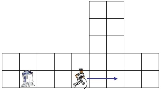
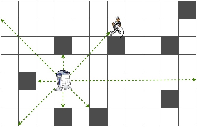
(a)	(b)
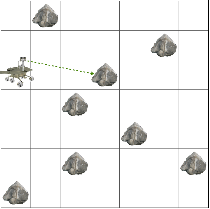
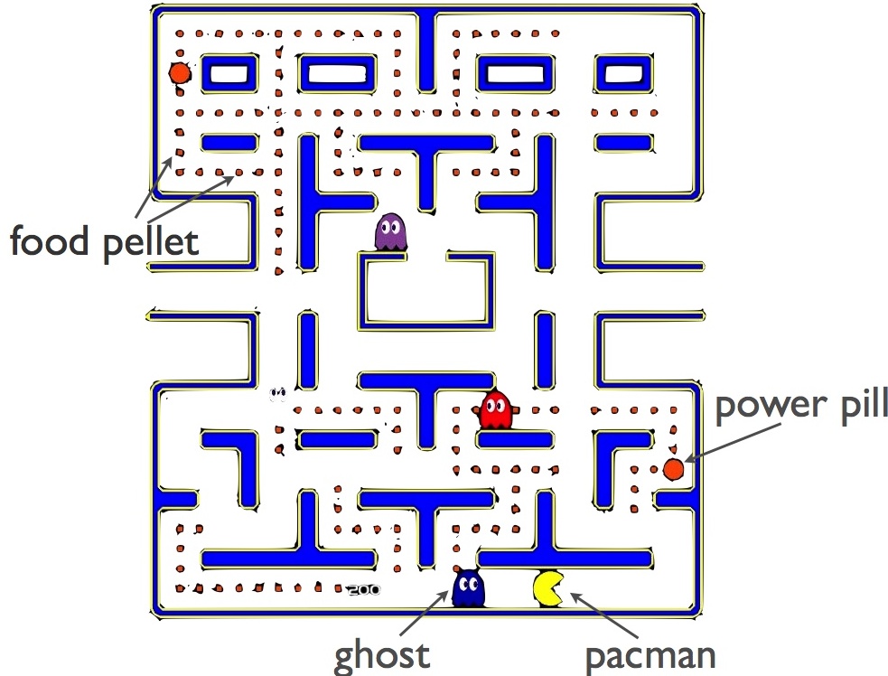
(c)	(d)

Figure 4: Four test domains. (a) Tag. A robot chases an unobserved target that runs away. (b) Laser Tag. A robot chases a target in a $7\times 11$ grid environment populated with obstacles. The robot is equipped with a laser range finder for self-localization. (c) Rock Sample. A robot rover senses rocks to identify “good” ones and samples them. Upon completion, it exits the east boundary. (d) The original Pacman game.

5.1.1 Tag

Tag is a standard POMDP benchmark introduced by ? (?). A robot and a target operate in a grid with 29 possible positions (Figure 4a). The robot’s goal is to find and tag the target that intentionally runs away. They start at random initial positions. The robot knows its own position, but can observe the target’s position only if they are in the same grid cell. The robot can either stay in the same position or move to the four adjacent positions, paying a cost of $-1$ for each move. It can also attempt to tag the target. It is rewarded $+10$, if the attempt is successful, and is penalized $-10$ otherwise. To complete the task successfully, a good policy exploits the target’s dynamics to “push” it against a corner of the environment.

For DESPOT, we use the hindsight optimization bound for the initial upper bound $U_{0}$ and initialize hindsight optimization by setting $U(D,s)$ to be the optimal MDP value (Section 4.3). We use the mode-MDP policy for the default policy $\pi_{0}$ (Section 4.4).

POMCP cannot use the mode-MDP policy, as it requires default policies that depend on the history only. We use the Tag implementation that comes as part of the authors’ POMCP package, but improved its default policy. The original default policy tags when both the robot and the target lie in a corner. Otherwise the robot randomly chooses an action that avoids doubling back or going into the walls. The improved policy tags whenever the agent and the target lie in the same grid cell, otherwise avoids doubling back or going into the walls, yielding better results based on our experiments.

On this moderate-size domain, SARSOP achieves the best result. AEMS2 and DESPOT have comparable performance. POMCP’s performance is much weaker, partly because of the limitation on its default policy.

5.1.2 Laser Tag

Theorem 3.1 suggests that DESPOT may perform well even when the observation space is large, provided that a small good policy exists. We now consider Laser Tag, an expanded version of Tag with a large observation space. In Laser Tag, the robot moves in a $7\times 11$ rectangular grid with obstacles placed randomly in eight grid cells (Figure 4b). The robot’s and target’s behaviors remain the same as before. However, the robot does not know its own position exactly and is distributed uniformly over the grid initially. To localize, it is equipped with a laser range finder that measures the distances in eight directions. The side length of each cell is 1. The laser reading in each direction is generated from a normal distribution centered at the true distance of the robot to the nearest obstacle in that direction, with a standard deviation of $2.5$. The readings are rounded to the nearest integers. So an observation comprises a set of eight integers, and the total number of observations is roughly $1.5\times 10^{6}$.

DESPOT uses a domain-specific method, which we call Shortest Path (SP) for the upper bound. For every possible initial target position, we compute an upper bound by assuming that the target stays stationary and that the robot follows a shortest path to tag the target. We then take the average over the sampled scenarios. DESPOT’s default policy is similar to the one used by POMCP in Tag, but it uses the most likely robot position to choose actions that avoid doubling back and running into walls. So it is not a scenario-based policy but a hybrid policy that makes use of both the belief and the history.

As the robot does not know its exact location, it is more difficult for POMCP’s default policy to avoid going into walls and doubling back. Hence, we only implemented the action of tagging whenever the robot and target are in the same location, and did not implement wall and doubling back avoidance.

With the very large observation space, we are not able to successfully run SARSOP and AEMS2. DESPOT achieves substantially better result than POMCP on this task.

5.1.3 Rock Sample

Next we consider Rock Sample, a well-established benchmark with a large state space (?). In RS$(n,k)$, a robot rover moves on an $n\times n$ grid containing $k$ rocks, each of which may be good or bad (Figure 4c). The robot’s goal is to visit and sample the good rocks, and exit the east boundary upon completion. At each step, the robot may move to an adjacent cell, sense a rock, or sample a rock. Sampling gives a reward of $+10$ if the rock is good and $-10$ otherwise. Moving and sensing have reward $0$. Moving or sampling do not produce any observation, or equivalently, null observation is produced. Sensing a rock produces an observation, GOOD or BAD, with probability of being correct decreasing exponentially with the robot’s distance from the rock. To obtain high total reward, the robot navigates the environment and senses rocks to identify the good ones; at the same time, it exploits the information gained to visit and sample the good rocks.

For upper bounds, DESPOT uses the MDP upper bound, which is a true upper bound in this case. For default policy, it uses a simple fixed-action default policy that always moves to the east.

POMCP uses the default policy described in (?). The robot travels from rock location to rock location. At each rock location, the robot samples the rock if there are more GOOD observations there than BAD observations. If all remaining rocks have a greater number of BAD observations, the robot moves to the east boundary and exits.

On the smallest domain RS$(7,8)$, the offline algorithm SARSOP obtains the best result overall. Among the three online algorithms, DESPOT has the best result. On RS$(11,11)$, DESPOT matches SARSOP in performance and is better than POMCP. On the largest instance RS$(15,15)$, SARSOP and AEMS2 cannot be completed successfully. It is also interesting to note that although the default policy for DESPOT is weaker than that of POMCP, DESPOT still achieves better results.

5.1.4 Pocman

Pocman (?) is a partially observable variant of the popular video game Pacman (Figure 4d). In Pocman, an agent and four ghosts move in a $17\times 19$ maze populated with food pellets. Each agent move incurs a cost of $-1$. Each food pellet provides a reward of $+10$. If the agent is captured by a ghost, the game terminates with a penalty of $-100$. In addition, there are four power pills. Within the next 15 time steps after eating a power pill, the agent can eat a ghost encountered and receives a reward of $+25$. A ghost chases the agent if the agent is within a Manhattan distance of $5$, but runs away if the agent possesses a power pill. The agent does not know the exact ghost locations, but receives information on whether it sees a ghost in each of the cardinal directions, on whether it hears a ghost within a Manhattan distance of $2$, on whether it feels a wall in each of the four cardinal directions, and on whether it smells food pellets in adjacent or diagonally adjacent cells. Pocman has an extremely large state space of roughly $10^{56}$ states.

For DESPOT, we compute an approximate hindsight optimization bound at a DESPOT node $b$ by summing the following quantities for each scenario in ${\bm{\Phi}}_{b}$ and taking the average over all scenarios: the reward for eating each pellet discounted by its distance from pocman, the reward for clearing the level discounted by the maximum distance to a pellet, the default per-step reward of $-1$ for a number of steps equal to the maximum distance to a pellet, the penalty for eating a ghost discounted by the distance to the closest ghost being chased if any, the penalty for dying discounted by the average distance to the ghosts, and half the penalty for hitting a wall if the agent tries to double back along its direction of movement. Under the default policy, when the agent detects a ghost, it chases a ghost if it possess a power pill and runs away from the ghost otherwise. When the agent does not detect any ghost, it makes a random move that avoids doubling back or going into walls. Due to the large scale of this domain, we used $K=100$ scenarios in the experiments in order to stay within the allocated $1$ second online planning time. For this problem, POMCP uses the same default policy as DESPOT.

On this large-scale domain, DESPOT has slightly better performance than POMCP, while SARSOP and AEMS2 cannot run successfully.

5.1.5 Bridge Crossing

The experiments above indicate that both POMCP and DESPOT can handle very large POMDPs. However, the UCT search strategy (?) which POMCP depends on has very poor worst-case behavior (?). We designed Bridge Crossing, a very simple domain, to illustrate this.

In Bridge Crossing, a person attempts to cross a narrow bridge over a mountain pass in the dark. He starts out at one end of bridge, but is uncertain of his exact initial position because of the darkness. At any time, he may call for rescue and terminate the attempt. In the POMDP model, the man has $10$ discretized positions $x\in\{0,1,\ldots,9\}$ along the bridge, with the person at the end of $x=0$. He is uncertain about his initial position, with a maximum error of $1$. He can move forward or backward, with cost $-1$. However, moving forward at $x=9$ has cost $0$, indicating successful crossing. For simplicity, we assume no movement noise. The person can call for rescue, with cost $-x-20$, where $x$ is his current position. The person has no observations while in the middle of the bridge. His attempt terminates when he successfully crosses the bridge or calls for rescue.

DESPOT uses the uninformed upper bound and the trivial default policy of calling for rescue immediately. POMCP uses the same default policy.

This is an open-loop planning problem. A policy is simply a sequence of actions, as there are no observations. There are $3$ possible actions at each step, and thus when considering policies of length at most 10, there are at most $3^{1}+3^{2}+\ldots+3^{10}<3^{11}$ policies. A simple breadth-first enumeration of these policies is sufficient to identify the optimal one: keep moving forward for a maximum of $10$ steps. Indeed, both SARSOP and AEMS2 obtain this optimal policy, as does DESPOT. While the initial upper bound and the default policy for DESPOT are uninformed, the backup operations improve the bounds and guide the search towards the right direction to close the gap between the upper and lower bounds. In contrast, POMCP’s performance on this domain is poor, because it is misled by its default policy and has an extremely poor convergence rate for cases such as this. While the optimal policy is to move forward all the way, the Monte Carlo simulations employed by POMCP suggests doing exactly the opposite at each step—move backward and call for rescue—because calling for rescue early near the starting point incurs lower cost. Increasing the exploration constant $c$ may somewhat alleviate this difficulty, but does not resolve it substantively.

5.2 Benefits of Regularization

Table 2: Performance of DESPOT, with and without regularization. The table reports the average total discounted reward achieved. For Pocman, it reports the total undiscounted reward without discounting.

	Tag	Laser Tag	RS(7,8)	RS(11,11)	RS(15,15)	Pocman	Bridge Crossing
$|Z|$	30	$\sim 1.5\times 10^{6}$	3	3	3	1,024	1
$\lambda$	0.01	0.01	0.0	0.0	0.0	0.1	0.0
Regularized	$-6.23\pm 0.26$	$-8.45\pm 0.26$	$20.93\pm 0.30$	$21.75\pm 0.30$	$18.64\pm 0.28$	$317.78\pm 4.20$	$-7.40\pm 0.0$
Unregularized	$-6.48\pm 0.26$	$-9.95\pm 0.26$	$20.90\pm 0.30$	$21.75\pm 0.30$	$18.15\pm 0.29$	$269.64\pm 4.33$	$-7.40\pm 0.0$

We now study the effect of regularization on the performance of DESPOT. If a POMDP has a large number of observations, the size of the corresponding belief tree and the optimal policy may be large as well. Overfitting to the sampled scenarios is thus more likely to occur, and we would expect that regularization may help. Indeed, Table 2 shows that Tag, Rock Sample, and Bridge Crossing, which all have a small or moderate number of observations, do not benefit much from regularization. The remaining two, Laser Tag and Pocman, which have a large number of observations, benefit more significantly from regularization.

To understand better the underlying cause, we designed another simple domain, Adventurer, with a variable number of observations. An adventurer explores an ancient ruin modeled as a $1\times 5$ grid. He is initially located in the leftmost cell. The treasure is located in the rightmost cell, with value uniformly distributed over a finite set $X$. If the adventurer reaches the rightmost cell and stays there for one step to dig up the treasure, he receives the value of the treasure as the reward. The adventurer can drive left, drive right, or stay in the same place. Each move may severely damage his vehicle with probability $0.5$, because of the rough terrain. The damage incurs a cost of $-10$ and terminates the adventure. The adventurer has a noisy sensor that reports the value of the treasure at each time step. The sensor reading is accurate with probability $0.7$, and the noise is evenly distributed over other possible values in $X$. At each time step, the adventurer must decide, based on the sensor readings received so far, whether to drive on in hope of getting the treasure or to stay put and protect his vehicle. With a discount factor of 0.95, the optimal policy is in fact to stay in the same place.

We studied two settings empirically: $X=\{101,150\}$ and $X=\{101,102,\ldots,150\}$, which result in $2$ and $50$ observations, respectively. For each setting, we constructed 1,000 full DESPOTs from $K=500$ randomly sampled scenarios. We compute the optimal action without regularization for each DESPOT. In the first setting with 2 observations, the computed action is always to stay in the same place. This is indeed optimal. In the second setting with 50 observations, about half of the computed actions are to move right. This is suboptimal. Why did this happen?

Recall that the sampled scenarios are split among the observation branches. With $2$ observations, each observation branch has $250$ scenarios on average, after the first step. This is sufficient to represent the uncertainty well. With $50$ observations, each observation branch has only about $5$ scenarios on average. Because of the sampling variance, the algorithm easily underestimates the probability and the expected cost of damage to the vehicle. In other words, it overfits to the sampled scenarios. Overfitting thus occurs much more often with a large number of observations.

Regularization helps to alleviate overfitting. For the second setting, we ran the algorithm with and without regularization. Without regularization, the average total discounted reward is $-6.06\pm 0.24$. With regularization, the average total discounted reward is $0\pm 0$, which is optimal.

5.3 Effect of Initial Bounds

Both DESPOT and POMCP rely on Monte Carlo simulation as a key algorithmic technique. They differ in two main aspects. One is their search strategies. We have seen in Section 5.1 that POMCP’s search strategy is more greedy, while DESPOT’s search strategy is more robust. Another difference is their default policies. While POMCP requires history-based default policies, DESPOT provides greater flexibility. Here we look into the benefits of this flexibility and also illustrate several additional techniques for constructing effective default policies and initial upper bounds. The benefits of cleverly-crafted default policies and initial upper bounds are domain-dependent. We examine three domains — Tag, Laser Tag, and Pocman — to give some intuition. Tag and Laser Tag are closely related for easy comparison, and both Laser Tag and Pocman are large-scale domains. The results for Tag, Laser Tag, and Pocman are shown on Tables 3 and 4.

For Tag and Laser Tag, we considered the following default policies for both problems.

• NORTH is a domain-specific, fixed-action policy that always moves the robot to the adjacent grid cell to the north at every time step.

• HIST is the improved history-based policy used by POMCP in the Tag experiment (Section 5.1.1).

• HYBRID is the hybrid policy used by DESPOT in the Laser Tag experiment (Section 5.1.2).

• The mode-MDP policy is the scenario-based policy described in Section 4.4 and used by DESPOT in the Tag experiment (Section 5.1.1). It first estimates the most likely state and then applies the optimal MDP policy accordingly.

• MODE-SP is a variant of the MODE-MDP policy. Instead of the optimal MDP policy, it applies a handcrafted domain-specific policy, which takes the action that moves the robot towards the target along a shortest path in the most likely state.

Next, consider the initial upper bounds. UI is the uninformed upper bound (13). MDP is the MDP upper bound (16). SP is the domain-specific bound used in Laser Tag (Section 5.1.2). We can use any of these three bounds, UI, MDP, or SP, to initialize $U(D,s)$ and obtain a corresponding hindsight optimization bound.

Table 3: Comparison of different initial upper and default policies on Tag and Laser Tag. The table reports the average total discounted rewards of the default policies (column 2) and of DESPOT when used with different combinations of initial upper and default policies (columns 3–8).

Default Policy			Initial Upper Bound
			UI	MDP	SP	HO-UI	HO-MDP	HO-SP
Tag
NORTH	-19.80 $\pm$ 0.00		-15.29 $\pm$ 0.35	-6.27 $\pm$ 0.26	-6.31 $\pm$ 0.26	-6.39 $\pm$ 0.27	-6.49 $\pm$ 0.26	-6.45 $\pm$ 0.26
HIST	-14.95 $\pm$ 0.41		-8.29 $\pm$ 0.28	-7.36 $\pm$ 0.26	-7.25 $\pm$ 0.26	-7.34 $\pm$ 0.26	-7.41 $\pm$ 0.26	-7.41 $\pm$ 0.26
MODE-MDP	-9.31 $\pm$ 0.29		-6.29 $\pm$ 0.27	-6.27 $\pm$ 0.26	-6.24 $\pm$ 0.27	-6.28 $\pm$ 0.26	-6.23 $\pm$ 0.26	-6.32 $\pm$ 0.26
MODE-SP	-12.57 $\pm$ 0.34		-6.53 $\pm$ 0.27	-6.51 $\pm$ 0.27	-6.38 $\pm$ 0.26	-6.52 $\pm$ 0.27	-6.56 $\pm$ 0.27	-6.55 $\pm$ 0.26
Laser Tag
NORTH	-19.80 $\pm$ 0.00		-15.80 $\pm$ 0.35	-11.18 $\pm$ 0.28	-10.35 $\pm$ 0.26	-10.91 $\pm$ 0.27	-10.91 $\pm$ 0.27	-10.91 $\pm$ 0.27
HYBRID	-19.77 $\pm$ 0.27		-8.76 $\pm$ 0.25	-8.59 $\pm$ 0.26	-8.45 $\pm$ 0.26	-8.52 $\pm$ 0.25	-8.66 $\pm$ 0.26	-8.54 $\pm$ 0.26
MODE-MDP	-9.97 $\pm$ 0.25		-9.83 $\pm$ 0.25	-9.84 $\pm$ 0.25	-9.83 $\pm$ 0.25	-9.83 $\pm$ 0.25	-9.83 $\pm$ 0.25	-9.83 $\pm$ 0.25
MODE-SP	-10.07 $\pm$ 0.26		-9.63 $\pm$ 0.25	-9.63 $\pm$ 0.25	-9.63 $\pm$ 0.25	-9.63 $\pm$ 0.25	-9.63 $\pm$ 0.25	-9.63 $\pm$ 0.25

For Pocman, we considered three default policies. NORTH is the policy of always moving to cell to the north. RANDOM is the policy which moves randomly to a legal adjacent cell. REACTIVE is the policy described in Section 5.1.4. We also considered two initial upper bounds. UI is the uninformed upper bound (13). AHO is the approximate hindsight optimization bound described in Section 5.1.4.

Table 4: Comparison of different initial upper and default policies on Pocman. The table reports the average total undiscounted rewards of the default policies (column 2) and of DESPOT when used with different combinations of initial upper and default policies (columns 3–4).

Default Policy			Initial Upper Bound
			UI	AHO
NORTH	$-1253.91\pm 24.03$		$-82.09\pm 1.72$	$-8.04\pm 3.54$
RANDOM	$-72.68\pm 1.42$		$284.70\pm 4.45$	$202.21\pm 4.71$
REACTIVE	$80.93\pm 5.40$		$315.62\pm 4.16$	$317.78\pm 4.20$

The results in Tables 3 and 4 offer several observations. First, DESPOT’s online search considerably improves the default policy that it starts with, regardless of the specific default policy and upper bound used. This indicates the importance of online search. Second, while some initial upper bounds are approximate, they nevertheless yield very good results, even compared with true upper bounds. This is illustrated by the approximate MDP bounds for Tag and Laser Tag as well as the approximate hindsight optimization bound for Pocman. Third, the simple uninformed upper bound can sometimes yield good results, when paired with suitable default policies. Finally, these observations are consistent across domains of different sizes, e.g., Tag and Laser Tag.

In these examples, default policies seem to have much more impact than initial upper bounds do. It is also interesting to note that for LaserTag, HYBRID is one of the worst-performing default policies, but leads to the best performance ultimately. So a stronger default policy does not always lead to better performance. There are other factors that may affect the performance, and flexibility in constructing both the upper bounds and initial policies can be useful.

6 Discussion

One key idea of DESPOT is to use a set of randomly sampled scenarios as an approximate representation of uncertainty and plan over the sampled scenarios. This works well if there exists a compact, near-optimal policy. The basic idea extends beyond POMDP planning and applies to other planning tasks under uncertainty, e.g., MDP planning and belief-space MDP planning.

The search strategy of the anytime DESPOT algorithm has several desirable properties. It is asymptotically sound and complete (Theorem 4.2). It is robust against imperfect heuristics (Theorem 4.2). It is also flexible and allows easy incorporation of domain knowledge. However, there are many alternatives, e.g., the UCT strategy used in POMCP. While UCT has very poor performance in the worst case, it is simpler to implement, an important practical consideration. Further, it avoids the overhead of computing the upper and lower bounds during the search and thus could be more efficient in some cases. In practice, there is trade-off between simplicity and robustness.

Large observation spaces may cause DESPOT to overfit to the sampled scenarios (see Section 5.2) and pose a major challenge. Unfortunately, this may happen with many common sensors, such as cameras and laser range finders. Regularization alleviates the difficulty. We are currently investigating several other approaches: structure the observation space hierarchically and importance sampling.

The default policy plays an important role in DESPOT. A good default policy reduces the size of the optimal policy. It also helps guide the heuristic search in the anytime search algorithm. In practice, we want the default policy to incorporate as much domain knowledge as possible for good performance. Another interesting direction is to learn the default policy during the search.

7 Conclusions

This paper presents DESPOT, a new approach to online POMDP planning. The main underlying idea is to plan according to a set of sampled scenarios while avoiding overfitting to the samples. Theoretical analysis shows that a DESPOT compactly captures the “execution” of all policies under the sampled scenarios and yields a near-optimal policy, provided that there is a small near-optimal policy. The analysis provides the justification for our overall planning approach based on sampled scenarios and the need for regularization. Experimental results indicate strong performance of the anytime DESPOT algorithm in practice. On moderately-sized POMDPs, DESPOT is competitive with SARSOP and AEMS2, but it scales up much better. On large-scale POMDPs with up to $10^{56}$ states, DESPOT matches and sometimes outperforms POMCP.

Acknowledgments

The work was mainly performed while N. Ye was with the Department of Computer Science, National University of Singapore. We are grateful to the anonymous reviewers for carefully reading the manuscript and providing many suggestions which helped greatly in improving the paper. The work is supported in part by National Research Foundation Singapore through the SMART IRG program, US Air Force Research Laboratory under agreements FA2386-12-1-4031 and FA2386-15-1-4010, a Vice Chancellor’s Research Fellowship provided by Queensland University of Technology and an Australian Laureate Fellowship (FL110100281) provided by Australian Research Council.

A Proofs

Proof of Theorem 3.1

We will need the following lemma from (?, p. 103) Lemma 9, part (2).

Lemma A.1.

(Haussler’s bound) Let $Z_{1},\ldots,Z_{n}$ be i.i.d random variables with range $0\leq Z_{i}\leq M$, $\mathbb{E}(Z_{i})=\mu$, and $\hat{\mu}=\frac{1}{n}\operatorname*{\sum}_{i=1}^{n}Z_{i}$, $1\leq i\leq n$. Assume $\nu>0$ and $0<\alpha<1$. Then

$$\Pr\left(d_{\nu}(\hat{\mu},\mu)>\alpha\right)<2e^{-\alpha^{2}{\nu}n/M}$$

where $d_{\nu}(r,s)=\frac{|r-s|}{\nu+r+s}$. As a consequence,

$$\Pr\left(\mu<\frac{1-\alpha}{1+\alpha}\hat{\mu}-\frac{\alpha}{1+\alpha}\nu\right)<2e^{-\alpha^{2}{\nu}n/M}.$$

Let $\Pi_{i}$ be the class of policy trees in $\Pi_{b_{0},0pt,K}$ and having size $i$. The next lemma bounds the size of $\Pi_{i}$.

Lemma A.2.

$|\Pi_{i}|\leq i^{i-2}(|A||Z|)^{i}$.

Proof.

Let $\Pi^{\prime}_{i}$ be the class of rooted ordered trees of size $i$. A policy tree in $\Pi_{i}$ is obtained from some tree in $\Pi^{\prime}_{i}$ by assigning one of the $|A|$ possible action labels to each node, and one of at most $|Z|$ possible labels to each edge, thus $|\Pi_{i}|\leq|A|^{i}\cdot|Z|^{i-1}$. $|\Pi^{\prime}_{i}|$. To bound $|\Pi^{\prime}_{i}|$, note that it is not more than the number of all trees with $i$ labeled nodes, because the in-order labeling of a tree in $\Pi^{\prime}_{i}$ corresponds to a labeled tree. By Cayley’s formula (?), the number of trees with $i$ labeled nodes is $i^{i-2}$, thus $|\Pi^{\prime}_{i}|\leq i^{(i-2)}$. Therefore $|\Pi_{i}|\leq i^{i-2}\cdot|A|^{i}\cdot|Z|^{i-1}\leq i^{i-2}(|A||Z|)^{i}$.

In the following, we often abbreviate $V_{\pi}(b_{0})$ and $\hat{V}_{\pi}(b_{0})$ as $V_{\pi}$ and $\hat{V}_{\pi}$ respectively, since we will only consider the true and empirical values for a fixed but arbitrary $b_{0}$. Our proof follows a line of reasoning similar to that of ? (?).

Theorem.

3.1 For any $\tau,\alpha\in(0,1)$, any belief $b_{0}$, and any positive integers $D$ and $K$, with probability at least $1-\tau$, every DESPOT policy tree $\pi\in\Pi_{b_{0},0pt,K}$ satisfies

$$V_{\pi}(b_{0})\geq\frac{1-\alpha}{1+\alpha}\hat{V}_{\pi}(b_{0})-\frac{R_{\mathrm{max}}}{(1+\alpha)(1-\gamma)}\cdot\frac{\ln(4/\tau)+|\pi|\ln\bigl{(}KD|A||Z|\bigr{)}}{\alpha K},$$

where the random variable $\hat{V}_{\pi}(b_{0})$ is the estimated value of $\pi$ under the set of $K$ scenarios randomly sampled according to $b_{0}$.

Proof.

Consider an arbitrary policy tree $\pi\in\Pi_{b_{0},0pt,K}$. We know that for a random scenario ${\bm{\phi}}$ for the belief $b_{0}$, executing the policy $\pi$ w.r.t. ${\bm{\phi}}$ gives us a sequence of states and observations distributed according to the distributions $P(s^{\prime}|s,a)$ and $P(z|s,a)$. Therefore, for $\pi$, its true value $V_{\pi}$ equals $\mathbb{E}\left(V_{\pi,{\bm{\phi}}}\right)$, where the expectation is over the distribution of scenarios. On the other hand, since $\hat{V}_{\pi}=\frac{1}{K}\sum_{k=1}^{K}V_{\pi,{\bm{\phi}}_{k}}$, and the scenarios ${\bm{\phi}}_{1},{\bm{\phi}}_{2},\ldots,{\bm{\phi}}_{K}$ are independently sampled, Lemma A.1 gives

$$\Pr\left(V_{\pi}<\frac{1-\alpha}{1+\alpha}\hat{V}_{\pi}-\frac{\alpha}{1+\alpha}\epsilon_{|\pi|}\right)<2e^{-\alpha^{2}{\epsilon_{|\pi|}}K/M}$$ (17)

where $M=(R_{\max})/(1-\gamma)$, and $\epsilon_{|\pi|}$ is chosen such that

$$2e^{-\alpha^{2}{\epsilon_{|\pi|}}K/M}=\tau/(2|\pi|^{2}|\Pi_{|\pi|}|).$$ (18)

By the union bound, we have

$$\Pr\left(\exists\pi\in\Pi_{b_{0},0pt,K}\text{ such that }V_{\pi}<\frac{1-\alpha}{1+\alpha}\hat{V}_{\pi}-\frac{\alpha}{1+\alpha}\epsilon_{|\pi|}\right)$$

$$\leq\sum_{i=1}^{\infty}\sum_{\pi\in\Pi_{i}}\Pr\left(V_{\pi}<\frac{1-\alpha}{1+\alpha}\hat{V}_{\pi}-\frac{\alpha}{1+\alpha}\epsilon_{|\pi|}\right).$$

By the choice of $\epsilon_{i}$’s and Inequality (17), the right hand side of the above inequality is bounded by $\sum_{i=1}^{\infty}|\Pi_{i}|\cdot[\tau/(2i^{2}|\Pi_{i}|)]=\bm{\uppi}^{2}\tau/12<\tau$, where the well-known identity $\sum_{i=1}^{\infty}1/i^{2}=\bm{\uppi}^{2}/6$ is used. Hence,

$$\Pr\left(\exists\pi\in\Pi_{b_{0},0pt,K}\left[V_{\pi}<\frac{1-\alpha}{1+\alpha}\hat{V}_{\pi}-\frac{\alpha}{1+\alpha}\epsilon_{|\pi|}\right]\right)<\tau.$$ (19)

Equivalently, with probability $1-\tau$, every $\pi\in\Pi_{b_{0},0pt,K}$ satisfies

$$V_{\pi}\geq\frac{1-\alpha}{1+\alpha}\hat{V}_{\pi}-\frac{\alpha}{1+\alpha}\epsilon_{|\pi|}.$$ (20)

To complete the proof, we now give an upper bound on $\epsilon_{|\pi|}$. From Equation (18), we can solve for $\epsilon_{|\pi|}$ to get $\epsilon_{i}=\frac{R_{\max}}{\alpha(1-\gamma)}\cdot\frac{\ln(4/\tau)+\ln(i^{2}|\Pi_{i}|)}{\alpha K}$. For any $\pi$ in $\Pi_{b_{0},0pt,K}$, its size is at most $KD$, and $i^{2}|\Pi_{i}|\leq(i|A||Z|)^{i}\leq(KD|A||Z|)^{i}$ by Lemma A.2. Thus we have

$$\epsilon_{|\pi|}\leq\frac{R_{\max}}{\alpha(1-\gamma)}\cdot\frac{\ln(4/\tau)+|\pi|\ln(KD|A||Z|)}{\alpha K}.$$

Combining this with Inequality (20), we get

$$V_{\pi}\geq\frac{1-\alpha}{1+\alpha}\hat{V}_{\pi}-\frac{R_{\max}}{(1+\alpha)(1-\gamma)}\cdot\frac{\ln(4/\tau)+|\pi|\ln(KD|A||Z|)}{\alpha K}.$$

This completes the proof.

Proof of Theorem 3.2

We need the following lemma for proving Theorem 3.2.

Lemma A.3.

For a fixed policy $\pi$ and any $\tau\in(0,1)$, with probability at least $1-\tau$.

$$\hat{V}_{\pi}\geq V_{\pi}-\frac{R_{\max}}{1-\gamma}\sqrt{\frac{2\ln(1/\tau)}{K}}$$

Proof.

Let $\pi$ be a policy and $V_{\pi}$ and $\hat{V}_{\pi}$ as mentioned. Hoeffding’s inequality (?) gives us

$$\Pr\left(\hat{V}_{\pi}\geq V_{\pi}-\epsilon\right)\geq 1-e^{-K\epsilon^{2}/(2M^{2})},$$

where $M=R_{\max}/(1-\gamma)$.

Let $\tau=e^{-K\epsilon^{2}/(2M^{2})}$ and solve for $\epsilon$, then we get

$$\Pr\left(\hat{V}_{\pi}\geq V_{\pi}-\frac{R_{\max}}{1-\gamma}\sqrt{\frac{2\ln(1/\tau)}{K}}\right)\geq 1-\tau.$$

Theorem.

3.2 Let $\pi$ be an arbitrary policy at a belief $b_{0}$. Let $\Pi_{\mathcal{D}}$ be the set of policies derived from a DESPOT $\mathcal{D}$ that has height 0ptand is constructed from $K$ scenarios sampled randomly according to $b_{0}$. For any $\tau,\alpha\in(0,1)$, if

$$\small{\hat{}\pi}=\operatorname*{arg\,max}_{\pi^{\prime}\in\Pi_{\mathcal{D}}}\biggl{\{}\frac{1-\alpha}{1+\alpha}\hat{V}_{\pi^{\prime}}(b_{0})-\frac{R_{\max}}{(1+\alpha)(1-\gamma)}\cdot\frac{|\pi^{\prime}|\ln\bigl{(}KD|A||Z|\bigr{)}}{\alpha K}\biggr{\}},$$

then

with probability at least $1-\tau$.

Proof.

By Theorem 1, with probability at least $1-\tau/2$,

$$V_{\hat{\pi}}\geq\frac{1-\alpha}{1+\alpha}\hat{V}_{\hat{\pi}}-\frac{R_{\max}}{(1+\alpha)(1-\gamma)}\left[\frac{\ln(8/\tau)+|\hat{\pi}|\ln(KD|A||Z|)}{\alpha K}\right].\\$$

Suppose the above inequality holds on a random set of $K$ scenarios. Note that there is a $\pi^{\prime}\in\Pi_{b_{0},0pt,K}$ which is a subtree of $\pi$ and has the same trajectories on these scenarios up to depth $D$. By the choice of $\hat{\pi}$, it follows that the following hold on the same scenarios

$$V_{\hat{\pi}}\geq\frac{1-\alpha}{1+\alpha}\hat{V}_{\pi^{\prime}}-\frac{R_{\max}}{(1+\alpha)(1-\gamma)}\left[\frac{\ln(8/\tau)+|\pi^{\prime}|\ln(KD|A||Z|)}{\alpha K}\right].\\$$

In addition, $|\pi|\geq|\pi^{\prime}|$, and $\hat{V}_{\pi^{\prime}}\geq\hat{V}_{\pi}-\gamma^{D}(R_{max})/(1-\gamma)$ since $\pi^{\prime}$ and $\pi$ only differ from depth $D$ onwards, under the chosen scenarios. It follows that for these scenarios, we have

$$V_{\hat{\pi}}\geq\frac{1-\alpha}{1+\alpha}\left(\hat{V}_{\pi}-\gamma^{D}\frac{R_{max}}{1-\gamma}\right)-\frac{R_{\max}}{(1+\alpha)(1-\gamma)}\left[\frac{\ln(8/\tau)+|\pi|\ln(KD|A||Z|)}{\alpha K}\right].$$ (21)

Hence, the above inequality holds with probability at least $1-\tau/2$.

By Lemma A.3, with probability at least $1-\tau/2$, we have

$$\hat{V}_{\pi}\geq V_{\pi}-\frac{R_{\max}}{1-\gamma}\sqrt{\frac{2\ln(2/\tau)}{K}}.$$ (22)

By the union bound, with probability at least $1-\tau$, both Inequality (21) and Inequality (22) hold, which imply the inequality in the theorem holds. This completes the proof.

Proof of Theorem 4.1 and Theorem 4.2

Lemma.

4.1 For any DESPOT node $b$, if $E(b)>0$ and $a^{*}=\arg\max_{a\in A}\mu(b,a)$, then

$$E(b)\leq\sum_{z\in Z_{b,a^{*}}}E(b^{\prime}),$$

where $b^{\prime}=\tau(b,a^{*},z)$ is a child of $b$.

Proof.

Let $\mathrm{CH}(b,a^{*})$ be all the set of all $b^{\prime}$ of the form $b^{\prime}=\tau(b,a,z)$ for some $z\in Z_{b,a^{*}}$, that is, the set of children nodes of $b$ in the DESPOT tree. If $E(b)>0$, then $\mu(b)-\ell(b)>0$, and thus $\mu(b)\neq\ell_{0}(b)$. Hence we have

$$\mu(b)=\mu(b,a^{*})=\rho(b,a^{*})+\sum_{b^{\prime}\in\mathrm{CH}(b,a^{*})}\mu(b^{\prime}),\text{ and }$$

$$\ell(b)\geq\ell(b,a^{*})\geq\rho(b,a^{*})+\sum_{b^{\prime}\in\mathrm{CH}(b,a^{*})}\ell(b^{\prime}),$$

Subtracting the first equation by the second inequality, we have

$$\mu(b)-\ell(b)\leq\sum_{b^{\prime}\in\mathrm{CH}(b,a^{*})}[\mu(b^{\prime})-\ell(b^{\prime})].$$

Note that

$$\frac{|{\bm{\Phi}}_{b}|}{K}\cdot\xi\cdot\epsilon(b_{0})=\sum_{b^{\prime}\in\mathrm{CH}(b,a^{*})}\frac{|{\bm{\Phi}}_{b^{\prime}}|}{K}\cdot\xi\cdot\epsilon(b_{0}).$$

We have

$${\sum_{b^{\prime}\in\mathrm{CH}(b,a^{*})}[\mu(b^{\prime})-\ell(b^{\prime})-\frac{|{\bm{\Phi}}_{b^{\prime}}|}{K}\cdot\xi\cdot\epsilon(b_{0})]}\geq{\mu(b)-\ell(b)-\frac{|{\bm{\Phi}}_{b}|}{K}\cdot\xi\epsilon(b_{0})}.$$

That is, $E(b)\leq\sum_{b^{\prime}\in\mathrm{CH}(b,a^{*})}E(b^{\prime})$.

Lemma.

4.2 Let $b^{\prime}$ be an ancestor of $b$ in a DESPOT $\mathcal{D}$ and $\ell(b^{\prime},b)$ be the number of nodes on the path from $b^{\prime}$ to $b$. If

$$\frac{|{\bm{\Phi}}_{b^{\prime}}|}{K}\gamma^{0pt(b^{\prime})}(U(b^{\prime})-L_{0}(b^{\prime}))\leq\lambda\cdot\ell(b^{\prime},b),$$

then $b$ cannot be a belief node in an optimal regularized policy derived from $\mathcal{D}$.

Proof.

If $b$ is included in the policy $\pi$ maximizing the regularized utility, then for any node $b^{\prime}$ on the path from $b$ to the root, the subtree $\pi_{b^{\prime}}$ under $b^{\prime}$ satisfies

$$\frac{|{\bm{\Phi}}_{b^{\prime}}|}{K}\gamma^{0pt(b^{\prime})}U(b^{\prime})-\lambda|\pi_{b^{\prime}}|$$

$$\geq \frac{|{\bm{\Phi}}_{b^{\prime}}|}{K}\gamma^{0pt(b^{\prime})}\hat{V}_{\pi_{b^{\prime}}}(b^{\prime})-\lambda|\pi_{b^{\prime}}| U(b^{\prime})>\hat{V}_{\pi_{b^{\prime}}}(b^{\prime})$$ (since )

$$> \frac{|{\bm{\Phi}}_{b^{\prime}}|}{K}\gamma^{0pt(b^{\prime})}L_{0}(b^{\prime}), b^{\prime}$$ (since is not pruned)

which implies

$$\frac{|{\bm{\Phi}}_{b^{\prime}}|}{K}\gamma^{0pt(b^{\prime})}U(b^{\prime})-\lambda|\pi_{b^{\prime}}|>\frac{|{\bm{\Phi}}_{b^{\prime}}|}{K}\gamma^{0pt(b^{\prime})}L_{0}(b^{\prime}).$$

Rearranging the terms in the above inequality, we have

$$\frac{|{\bm{\Phi}}_{b^{\prime}}|}{K}\gamma^{0pt(b^{\prime})}[U(b^{\prime})-L_{0}(b^{\prime})]>\lambda|\pi_{b^{\prime}}|.$$

We have $\ell(b^{\prime},b)\leq|\pi_{b^{\prime}}|$ as $b$ is not pruned and thus $\pi_{b^{\prime}}$ need to include all nodes from $b^{\prime}$ to $b$. Hence,

$$\frac{|{\bm{\Phi}}_{b^{\prime}}|}{K}\gamma^{0pt(b^{\prime})}[U(b^{\prime})-L_{0}(b^{\prime})]>\lambda\cdot\ell(b^{\prime},b).$$

Theorem.

4.1 Suppose that $T_{\mathrm{max}}$ is bounded and that the anytime DESPOT algorithm terminates with a partial DESPOT $\mathcal{D}^{\prime}$ that has gap $\epsilon(b_{0})$ between the upper and lower bounds at the root $b_{0}$. The optimal regularized policy $\hat{\pi}$ derived from $\mathcal{D}^{\prime}$ satisfies

$$\nu_{\hat{\pi}}(b_{0})\geq\nu^{*}(b_{0})-\epsilon(b_{0})-\delta,\vspace*{0pt}$$

where $\nu^{*}(b_{0})$ is the value of an optimal regularized policy derived from the full DESPOT $\mathcal{D}$ at $b_{0}$.

Proof.

Let $U^{\prime}_{0}(b)=U_{0}(b)+\delta$, then $U^{\prime}_{0}$ is an exact upper bound. Let $\mu^{\prime}_{0}$ be the corresponding initial upper bound, and $\mu^{\prime}$ be the corresponding upper bound on $\nu^{*}(b)$. Then $\mu^{\prime}_{0}$ is a valid initial upper bound for $\nu^{*}(b)$ and the backup equations ensure that $\mu^{\prime}(b)$ is a valid upper bound for $\nu^{*}(b)$. On the other hand, it can be easily shown by induction that $\mu(b)+\gamma^{0pt(b)}\frac{|{\bm{\Phi}}_{b}|}{K}\delta\geq\mu^{\prime}(b)$. As a special case for $b=b_{0}$, we have $\mu(b)+\delta\geq\mu^{\prime}(b_{0})$. Hence, when the algorithm terminates, we also have $\mu(b_{0})+\delta\geq\mu^{\prime}(b_{0})\geq\nu^{*}(b_{0})$. Equivalently, $\nu_{\hat{\pi}}=\ell(b_{0})\geq\nu^{*}(b_{0})-(\mu(b_{0})-\ell(b_{0}))-\delta=\nu^{*}(b_{0})-\epsilon(b_{0})-\delta$. The first equality holds because the initialization and the computation of the lower bound $\ell$ via the backup equations are exactly that for finding an optimal regularized policy value in the partial DESPOT.

Theorem.

4.2 Suppose that $T_{\mathrm{max}}$ is unbounded and $\epsilon_{0}$ is the target gap between the upper and lower bound at the root of the partial DESPOT constructed by the anytime DESPOT algorithm. Let $\nu^{*}(b_{0})$ be the value of an optimal policy derived from the full DESPOT $\mathcal{D}$ at $b_{0}$.

• If $\epsilon_{0}>0$, then the algorithm terminates in finite time with a near-optimal policy $\hat{}\pi$ satisfying

  $$\nu_{\hat{\pi}}(b_{0})\geq\nu^{*}(b_{0})-\epsilon_{0}-\delta.\vspace*{0pt}$$

• If $\epsilon_{0}=0$, $\delta=0$, and the regularization constant $\lambda>0$, then the algorithm terminates in finite time with an optimal policy $\hat{}\pi$, i.e., $\nu_{\hat{\pi}}(b_{0})=\nu^{*}(b_{0})$.

Proof.

(1) It suffices to show that eventually $\mu(b_{0})-\ell(b_{0})\leq\epsilon_{0}$, which then implies $\nu_{\hat{\pi}}(b_{0})\geq\nu^{*}(b_{0})-\epsilon_{0}-\delta$ by Theorem 4.1.

We first show that only nodes within certain depth $d_{0}$ will ever be expanded. In particular, we can choose any $d_{0}>0$ such that $\xi\epsilon_{0}>\gamma^{d_{0}}R_{max}/(1-\gamma)$. For any node $b$ beyond depth $d_{0}$, we have $\epsilon(b)\leq\gamma^{0pt(b)}\frac{|{\bm{\Phi}}_{b}|}{K}\frac{R_{max}}{1-\gamma}\leq\gamma^{d_{0}}\frac{|{\bm{\Phi}}_{b}|}{K}\frac{R_{max}}{1-\gamma}<\frac{|{\bm{\Phi}}_{b}|}{K}\cdot\xi\cdot\epsilon_{0}$. Since $\epsilon(b_{0})>\epsilon_{0}$ before the algorithm terminates, we have $E(b)=\epsilon(b)-\frac{|{\bm{\Phi}}_{b}|}{K}\cdot\xi\cdot\epsilon(b_{0})<\epsilon(b)-\frac{|{\bm{\Phi}}_{b}|}{K}\cdot\xi\cdot\epsilon_{0}<0$, and $b$ will not be expanded during the search.

On the other hand, the forward search heuristic guarantees that each exploration closes the gap of at least one node or expands at least one node. To see this, note that an exploration terminates when its depth exceeds the limit $D$, or when a node is pruned, or when it encounters a node $b$ with $E(b)<0$. In the first two cases, the gap for the last node is closed. We show that for the last case, the exploration must have expanded at least one node. By Lemma 4.1, if $E(b)>0$, then the next chosen node $b^{\prime}$ satisfies $E(b^{\prime})>0$, otherwise the upper bound for $E(b)$ will be at most 0, a contradiction. Since the root $b_{0}$ has positive $E$, thus the exploration will follow a path with nodes with positive $E$ to reach a leaf node, and then expand it. Termination may then happen as the next chosen node has negative $E$.

Since each node can be expanded or closed at most once, but only nodes within depth $d_{0}$ can be considered, thus after finitely many steps $\epsilon(b_{0})=\mu(b_{0})-\ell(b_{0})\leq\epsilon_{0}$, and the search terminates.

(2) Following the proof of (1), when $\epsilon=0$, before $\mu(b_{0})=\ell(b_{0})$, each exploration either closes the gap of at least one node, or expands at least one leaf node. However, both can only be done finitely many times because the Prune procedure ensures only nodes within a depth of $\lceil\frac{R_{max}}{\lambda(1-\gamma)}\rceil+1$ can be expanded, and the gap of each such node can only be closed once only. Thus the search will terminate in finite time with $\mu(b_{0})=\ell(b_{0})$. Since the upper bound is a true one, we have $\nu_{\hat{\pi}}(b_{0})=\ell(b_{0})=\nu^{*}(b_{0})$, and thus $\hat{\pi}$ is an optimal regularized policy derived from the infinite horizon DESPOT.

B Pseudocode for Anytime DESPOT

Algorithm 6 Anytime DESPOT

Input

• Initial belief.

• The target gap between $\mu(b_{0})$ and $\ell(b_{0})$.

• The rate of target gap reduction.

• The number of sampled scenarios.

• The maximum depth of the DESPOT.

• Regularization constant.

• The maximum online planning time per step.

1:  Initialize ${b}\leftarrow\beta$.

2:  loop

3:     $\ell\leftarrow\textsc{BuildDespot(${b}$)}$.

4:     $a^{*}\leftarrow\max_{a\in A}\ell({b},a)$.

5:     if $L_{0}({b})>\ell({b},a^{*})$ then

6:        $a^{*}\leftarrow\pi_{0}({b})$

7:     Execute $a^{*}$.

8:     Receive observation $z$.

9:     ${b}\leftarrow\tau({b},a^{*},z)$.

$\textsc{BuildDespot}({b}_{0})$

1:  Sample randomly a set ${\bm{\Phi}}_{{b}_{0}}$ of $K$ scenarios from the current belief ${b}_{0}$.

2:  Create a new DESPOT $\mathcal{D}$ with a single node ${b}$ as the root.

3:  Initialize $U({b}_{0}),L_{0}({b}_{0}),\mu({b}_{0}),\text{ and }\ell({b}_{0})$.

4:  $\epsilon({b}_{0})\leftarrow\mu({b}_{0})-\ell({b}_{0})$.

5:  while $\epsilon({b}_{0})>\epsilon_{0}$ and the total running time is less than $T_{\mathrm{max}}$ do

6:     $b\leftarrow\textsc{Explore}(\mathcal{D},{b}_{0})$.

7:     $\textsc{Backup}(\mathcal{D},b)$.

8:     $\epsilon({b}_{0})\leftarrow\mu({b}_{0})-\ell({b}_{0})$.

9:  return  $\ell$

$\textsc{Explore}(\mathcal{D},b)$

1:  while $0pt(b)\leq D$, $E(b)>0$, and Prune($\mathcal{D}$, $b$) = FALSE do

2:     if $b$ is a leaf node in $\mathcal{D}$ then

3:        Expand $b$ one level deeper. Insert each new child $b^{\prime}$ of $b$ into $\mathcal{D}$, and initialize $U(b^{\prime})$, $L_{0}(b^{\prime})$, $\mu(b^{\prime})$, and $\ell(b^{\prime})$.

4:     $a^{*}\leftarrow\operatorname*{arg\,max}_{a\in A}{\mu(b,a)}$.

5:     $z^{*}\leftarrow\operatorname*{arg\,max}_{z\in Z_{b,a^{*}}}E(\tau(b,a^{*},z))$.

6:     $b\leftarrow\tau(b,a^{*},z^{*})$.

7:  if $0pt(b)>D$ then

8:     MakeDefault($b$).

9:  return  $b$.

Prune($\mathcal{D},b$)

1:  $\textsc{Blocked}\leftarrow\text{\small FALSE}$.

2:  for each node $x$ on the path from $b$ to the root of $\mathcal{D}$ do

3:     if $x$ is blocked by any ancestor node in $\mathcal{D}$ then

4:        MakeDefault($x$);

5:        Backup($\mathcal{D}$, $x$).

6:        $\textsc{Blocked}\leftarrow\text{\small TRUE}$.

7:     else

8:        break

9:  return  Blocked

MakeDefault($b$)

1:  $U(b)\leftarrow L_{0}(b)$.

2:  $\mu(b)\leftarrow\ell_{0}(b)$.

3:  $\ell(b)\leftarrow\ell_{0}(b)$.

Backup($\mathcal{D},b$)

1:  for each node $x$ on the path from $b$ to the root of $\mathcal{D}$ do

2:     Perform backup on $\mu(x)$, $\ell(x)$, and $U(x)$.

References

- Bai, Hsu, Lee, and Ngo Bai, H., Hsu, D., Lee, W. S., and Ngo, V. (2011). Monte carlo value iteration for continuous-state POMDPs. Algorithmic Foundations of Robotics IX, 175–191.
- Bai, Cai, Ye, Hsu, and Lee Bai, H., Cai, S., Ye, N., Hsu, D., and Lee, W. (2015). Intention-Aware Online POMDP Planning for Autonomous Driving in a Crowd. In Proc. IEEE Int. Conf. on Robotics & Automation.
- Bertsekas and Castanon Bertsekas, D. P., and Castanon, D. A. (1999). Rollout algorithms for stochastic scheduling problems. J. Heuristics, 5(1), 89–108.
- Cayley Cayley, A. (1889). A Theorem on Trees. Quart. J. Math, 23, 376–378.
- Chadès, Carwardine, Martin, Nicol, Sabbadin, and Buffet Chadès, I., Carwardine, J., Martin, T., Nicol, S., Sabbadin, R., and Buffet, O. (2012). MOMDPs: A Solution for Modelling Adaptive Management Problems. In Proc. AAAI Conf. on Artificial Intelligence.
- Chong, Givan, and Chang Chong, E., Givan, R., and Chang, H. (2000). A framework for simulation-based network control via hindsight optimization. In Proc. IEEE Conf. on Decision & Control, Vol. 2, pp. 1433–1438.
- Coquelin and Munos Coquelin, P.-A., and Munos, R. (2007). Bandit algorithms for tree search. In Proc. Conf. on Uncertainty in Artificial Intelligence.
- Gelly and Silver Gelly, S., and Silver, D. (2007). Combining online and offline knowledge in UCT. In Proc. Int. Conf. on Machine Learning.
- Gordon, Salmond, and Smith Gordon, N., Salmond, D., and Smith, A. (1993). Novel approach to nonlinear/non-Gaussian Bayesian state estimation. IEE Proc. F on Radar & Signal Processing, 140(2), 107–113.
- Hauskrecht and Fraser Hauskrecht, M., and Fraser, H. (2000). Planning treatment of ischemic heart disease with partially observable Markov decision processes. Artificial Intelligence in Medicine, 18(3), 221–244.
- Haussler Haussler, D. (1992). Decision theoretic generalizations of the PAC model for neural net and other learning applications. Information and Computation, 100(1), 78–150.
- He, Brunskill, and Roy He, R., Brunskill, E., and Roy, N. (2011). Efficient planning under uncertainty with macro-actions. J. Artificial Intelligence Research, 40(1), 523–570.
- Hoeffding Hoeffding, W. (1963). Probability inequalities for sums of bounded random variables. J. American statistical association, 58(301), 13–30.
- Kaelbling, Littman, and Cassandra Kaelbling, L. P., Littman, M. L., and Cassandra, A. R. (1998). Planning and acting in partially observable stochastic domains. Artificial intelligence, 101(1), 99–134.
- Kearns, Mansour, and Ng Kearns, M., Mansour, Y., and Ng, A. (1999). Approximate planning in large POMDPs via reusable trajectories. In Advances in Neural Information Processing Systems (NIPS), Vol. 12, pp. 1001–1007.
- Kearns, Mansour, and Ng Kearns, M., Mansour, Y., and Ng, A. Y. (2002). A sparse sampling algorithm for near-optimal planning in large Markov decision processes. Machine Learning, 49(2-3), 193–208.
- Kocsis and Szepesvari Kocsis, L., and Szepesvari, C. (2006). Bandit based Monte-Carlo planning. In Proc. Eur. Conf. on Machine Learning, pp. 282–293.
- Kurniawati, Hsu, and Lee Kurniawati, H., Hsu, D., and Lee, W. (2008). SARSOP: Efficient point-based POMDP planning by approximating optimally reachable belief spaces. In Proc. Robotics: Science and Systems.
- Lusena, Goldsmith, and Mundhenk Lusena, C., Goldsmith, J., and Mundhenk, M. (2001). Nonapproximability results for partially observable Markov decision processes. J. Artif. Intell. Res. (JAIR), 14, 83–103.
- Madani, Hanks, and Condon Madani, O., Hanks, S., and Condon, A. (1999). On the undecidability of probabilistic planning and infinite-horizon partially observable Markov decision problems. In Proc. AAAI Conf. on Artificial Intelligence, pp. 541–548.
- Ng and Jordan Ng, A., and Jordan, M. (2000). PEGASUS: A policy search method for large MDPs and POMDPs. In Proc. Conf. on Uncertainty in Artificial Intelligence, pp. 406–415.
- Papadimitriou and Tsitsiklis Papadimitriou, C. H., and Tsitsiklis, J. N. (1987). The complexity of Markov decision processes. Mathematics of Operations Research, 12(3), 441–450.
- Paquet, Tobin, and Chaib-Draa Paquet, S., Tobin, L., and Chaib-Draa, B. (2005). An online POMDP algorithm for complex multiagent environments. In Proceedings of the fourth international joint conference on Autonomous agents and multiagent systems, pp. 970–977. ACM.
- Pineau, Gordon, and Thrun Pineau, J., Gordon, G., and Thrun, S. (2003). Point-based value iteration: An anytime algorithm for POMDPs. In Proc. Int. Jnt. Conf. on Artificial Intelligence, pp. 477–484.
- Poupart Poupart, P. (2005). Exploiting structure to efficiently solve large scale partially observable Markov decision processes. Ph.D. thesis, University of Toronto.
- Ross and Chaib-Draa Ross, S., and Chaib-Draa, B. (2007). AEMS: An anytime online search algorithm for approximate policy refinement in large POMDPs. In Proc. Int. Jnt. Conf. on Artificial Intelligence, pp. 2592–2598.
- Ross, Pineau, Paquet, and Chaib-Draa Ross, S., Pineau, J., Paquet, S., and Chaib-Draa, B. (2008). Online planning algorithms for POMDPs. J. Artificial Intelligence Research, 32(1), 663–704.
- Roy, Burgard, Fox, and Thrun Roy, N., Burgard, W., Fox, D., and Thrun, S. (1999). Coastal navigation: mobile robot navigation with uncertainty in dynamic environments. In Proc. IEEE Int. Conf. on Robotics & Automation.
- Satia and Lave Satia, J., and Lave, R. (1973). Markovian decision processes with probabilistic observation of states. Management Science, 20(1), 1–13.
- Silver and Veness Silver, D., and Veness, J. (2010). Monte-Carlo planning in large POMDPs. In Advances in Neural Information Processing Systems (NIPS).
- Smallwood and Sondik Smallwood, R. D., and Sondik, E. J. (1973). The optimal control of partially observable Markov processes over a finite horizon. Operations Research, 21(5), 1071–1088.
- Smith and Simmons Smith, T., and Simmons, R. (2004). Heuristic search value iteration for POMDPs. In Proc. Conf. on Uncertainty in Artificial Intelligence, pp. 520–527.
- Smith and Simmons Smith, T., and Simmons, R. (2005). Point-based POMDP algorithms: Improved analysis and implementation. In Proc. Conf. on Uncertainty in Artificial Intelligence.
- Somani, Ye, Hsu, and Lee Somani, A., Ye, N., Hsu, D., and Lee, W. (2013). DESPOT: POMDP planning with regularization. In Advances in Neural Information Processing Systems (NIPS).
- Spaan and Vlassis Spaan, M., and Vlassis, N. (2005). Perseus: Randomized point-based value iteration for POMDPs. J. Artificial Intelligence Research, 24, 195–220.
- Wang, Won, Hsu, and Lee Wang, Y., Won, K., Hsu, D., and Lee, W. (2012). Monte Carlo Bayesian reinforcement learning. In Proc. Int. Conf. on Machine Learning.
- Yoon, Fern, Givan, and Kambhampati Yoon, S., Fern, A., Givan, R., and Kambhampati, S. (2008). Probabilistic planning via determinization in hindsight. In Proc. AAAI Conf. on Artificial Intelligence.
- Zhang and Zhang Zhang, N., and Zhang, W. (2001). Speeding Up the Convergence of Value Iteration in Partially Observable Markov Decision Processes. J. Artificial Intelligence Research, 14, 29–51.