Machine-learning Selection of Optical Transients in Subaru/Hyper Suprime-Cam Survey

Abstract

We present an application of machine-learning (ML) techniques to source selection in the optical transient survey data with Hyper Suprime-Cam (HSC) on the Subaru telescope. Our goal is to select real transient events accurately and in a timely manner out of a large number of false candidates, obtained with the standard difference-imaging method. We have developed the transient selector which is based on majority voting of three ML machines of AUC Boosting, Random Forest, and Deep Neural Network. We applied it to our observing runs of Subaru-HSC in 2015 May and August, and proved it to be efficient in selecting optical transients. The false positive rate was 1.0% at the true positive rate of 90% in the magnitude range of 22.0–25.0 mag for the former data. For the latter run, we successfully detected and reported ten candidates of supernovae within the same day as the observation. From these runs, we learned the following lessons: (1) the training using artificial objects is effective in filtering out false candidates, especially for faint objects, and (2) combination of ML by majority voting is advantageous.

1 Introduction

The 8.2-m Subaru telescope has been running a 300-night Strategic Survey Program (SSP) over 5 years since 2014 March, in order to elucidate the mystery of dark matter and dark energy as well as the evolution of galaxies. The survey utilizes Hyper Suprime-Cam (HSC; [Miyazaki et al. (2012)]) with a wide field of view of 1.77 square degrees. In 2016–18, we observe two ultra deep fields, COSMOS and SXDS, for six-month each. The observations will be performed around the new moon in each month, with a typical cadence of 3–4 days. Note that the HSC is not installed on Subaru for two weeks around the full moon. Among other transient surveys, the Subaru HSC/SSP survey is the deepest for this survey area ($1.77\times 2$ square degrees), and thus, will provide the unique dataset for transients. For example, the HSC/SSP survey will triple the number of type-Ia supernovae (SNe) beyond redshift $z>1$ and will also discover a few tens of superluminous SNe at $z>1$.

Difference imaging is the standard method to search for optical transient objects, and so we use it in this study. We define a transient object as the one that appears only in the image at the later epoch (newer image), but not in the one at the earlier epoch (reference image or template image), out of the two images taken at different epochs. After the standard data reduction is made, two images are astrometrically aligned, and the reference image is subtracted from the newer image by matching point spread functions (PSFs) of the two images. The source-finding algorithm is applied to the difference image, and the detected sources are the candidates of transients (section 2).

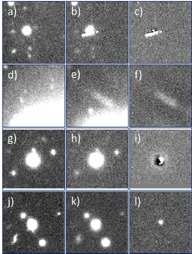
Figure 1: Examples of real and bogus objects obtained with Subaru-HSC. The left, middle, and right columns show the reference, new, and difference images, respectively. The first, second, and third rows show the cosmic ray (a–c), ghost near a bright star (d–f), and inaccurate image convolution or astrometric alignment (g–i), respectively. The bottom row shows a real transient located in a galaxy (j–l).

In an ideal situation, all the sources detected in difference images would be transient/variable astronomical sources, such as supernovae, variable stars, moving objects, and so on. In reality, however, they also include artifacts (see panels a–i in figure 1), such as cosmic-ray events, spikes around bright stars, and residuals related to inaccurate image convolution or astrometric alignment. These artifacts are present in every optical survey project (Bailey et al., 2007; Bloom et al., 2012; Brink et al., 2013). Hereafter, we call them “bogus” (Bloom et al., 2012).

In the HSC/SSP survey, not only a few hundred transients, including SNe, but also $\sim 10^{5}-10^{6}$ bogus objects are expected to be detected each night. After the scheduled 300 nights, the number of candidates of transients, real and bogus combined, will reach $\sim 10^{8}$, which is well qualified as Big Data. We need to filter out bogus objects to select SNe and other real transients. Processing of filtering must be performed swiftly in order to increase the chances of new findings in an early phase of transient phenomena.

The primary method to distinguish transient/bogus objects is, traditionally, visual inspection by human checkers, as many surveys have been adopting. However, the expected size of our data is so big that human checkers would not be able to go through all the data in a reasonable time. We have decided to introduce machine-learning (ML) techniques to select real transients.

In the filtering process, we should not miss real objects, while a vast number of bogus objects are filtered out. Throughout the development, we try to minimize the false positive rate (FPR), while we maintain the true positive rate (TPR) of 90 % or larger (namely the false negative rate, FNR $<10\%$).

We performed two HSC observations in 2015 May and August (Tominaga et al., 2015b, c), aiming to detect short transients with a time scale of a few hours to a few days (e.g. Tanaka et al. (2016); Morokuma et al. (2016)). An example of such short transients is an optical flash at the time of shock breakout of a supernova, of which the time-variance would be detectable during an observation for a single night. We use three kinds of ML methods, AUC Boosting, Random Forests (RF), and Deep Neural Network (DNN), both individually and in a combined way. We verify the performance of these machines by making the receiver operation characteristic (ROC) curves.

Conditions of observations (the noise and seeing) vary every night. Hence, the ML classifiers must be robust against the change of environment. We use normalized features to reduce the influence of the variation. To validate the performance of our method, we show the ROC curves of our machine trained with the data on one-night observation, applied to the data on the other night observation. The results show the proposed classifier is robust.

In optical surveys, ML techniques have been introduced by Bailey et al. (2007) for the data from the Nearby Supernova Factory. They applied Boosted Decision Trees, RF, and Support Vector Machines (SVM) and succeeded in reducing the number of bogus candidates by a factor of ten. The Palomar Transient Factory team (Bloom et al., 2012) used RF, and achieved the TPR of 92.3% at the FPR of 1% (Brink et al., 2013). The Pan-STARRS1 Medium Deep Survey used Artificial Neural Network, SVM and RF, and achieved TPR of 90% at FPR of 1% (Wright et al., 2015). Goldstein et al. (2015) applied the RF for Dark Energy Survey Supernova program (DES-SN), and reduced the number of transient candidates by a factor of 13.4, which were then fed to human scanning. du Buisson et al. (2015) applied the RF, $k$-nearest neighbor, and the SkyNet artificial neural net algorithm, using features trained from eigen-image analysis for the Sloan Digital Sky Survey supernova survey.

The rest of this paper is structured as follows. In section 2, we explain the HSC data reduction and feature extractions. In section 3, we introduce three machine learning methods we used. In section 4, the applications to the actual Subaru data are presented, and then we discuss the result of real vs bogus segregation in section 5.

Prior to the forthcoming HSC/SSP Transient survey, this paper will provide a ‘path finder’ to identify real astronomical objects and to demonstrate the power of machine learning.

2 Data Analysis and Feature Extraction

ll List of the features Feature variable Description
mag Magnitude
magerr Error of magnitude
elongation_norm Elongation normalized by nearby stars
fwhm_norm FWHM normalized by nearby stars
significance_abs Significance obtained with the PSF fit
residual Residual of PSF fit
psffit_sigma_ratio See text
psffit_peak_ratio See text
frac_det See text
density Number of objects around the target within a square with 120 $\times$ 120 pixels centered at the target
density_good “Density” after weak screening
bapsf Elongation of nearby stars
psf FWHM of nearby stars

We describe the flow of HSC data reduction and feature extraction for machine learning. The pipeline processing, using the on-site data analysis system (Furusawa et al., 2011), and then transient finding (Tominaga et al., 2015a), are performed immediately after the data acquisition.

The HSC data are reduced with the HSC pipeline (version 3.6.1), which has been developed based on the LSST pipeline (Ivezic et al., 2008; Axelrod et al., 2010). First, the pipeline performs the standard reduction, such as bias subtraction and flat fielding. Then, astrometric and photometric calibrations are made, using the Sloan Digital Sky Survey DR8 data (Aihara et al., 2011). Finally, mosaic solution is derived and images are warped to align astrometrically in preparation for co-adding (if needed) and image subtraction for difference-imaging at the next stage.

For image subtraction we use the HSC pipeline. The algorithm to match the PSFs of the two images is the same as that by Alard & Lupton (1998) and Alard (2000) , and adopts a position-dependent convolution kernel. The optimal convolution kernel is derived so that the difference between convoluted PSFs becomes the smallest. The algorithm has been implemented also in the HOTPANTS package .

Source detection is performed in difference images, using the HSC pipeline instead of the standard tool for it, SExtractor (Bertin & Arnouts, 1996), because the former outperforms the latter in reducing bogus detections.
For each source, the features listed in table 2 are computed as follows. We fit the image with the PSF of two-dimensional Gaussian and subtract the best-fit PSF from it. Then, we measure the residuals within 2 $\times$ FWHM radius ($\sigma_{\rm on}$) and in the surrounding region (3–4 $\times$ FWHM, $\sigma_{\rm off}$). We define “psffit$\_$sigma$\_$ratio” $=\sigma_{\rm on}/\sigma_{\rm off}$; it is expected to be much larger than unity when the shape of a source is very different from PSF. We also define “psffit$\_$peak$\_$ratio”, the ratio of the actual peak of the source to the peak of the best-fit Gaussian in order to quantify the degree of deviation of the source-image shape from the PSF.

To obtain features sensitive to mis-alignment, we count the number of positive pixels within $3\times$ FWHM, and define “frac$\_$posi” as their fraction. This feature frac$\_$posi should be close to unity for good detection with a high S/N ratio. Similarly, we count the number of negative pixels and define “frac$\_$nega” for its ratio to detect “sources” with negative counts. To use both the cases in a consistent manner, we define “frac$\_$det”, which is the same as “frac$\_$posi” for the positive detection but ($1-$ “frac$\_$nega”) for the negative detection. Following Bloom et al. (2012) and Brink et al. (2013), we also count the number of the detected sources inside a 120 $\times$ 120 pixel box centered at the source (“density”).

In the HSC pipeline, PSF fitting for the detected sources is performed with the position-dependent PSF. We also compute the significance of detection (significance$\_$abs) by comparing the fitted PSF with the noise level around a source.

In total, 13 features are used for machine learning (table 2).

3 Methods of Machine Learning for Real-Bogus Separation

3.1 AUC Boosting

Boosting is a method to classify the data by majority-voting of weak classifiers (Hastie, Tibshirani & Friedman, 2009). Among various boosting methods, we employed the AUC boosting developed by Komori (2011), which is trained to maximize the empirical area under the ROC curve (AUC). The AUC boosting classifies objects according to a score function, where the objects with larger scores are regarded as real. This method uses only one hyper-parameter $\lambda$ to control the smoothness of the score function, which is optimized through cross-validation.

Once the machine has been trained, classification for a new set of feature variables will be fast. Hence, when the trained machine is installed in the pipeline process of HSC, real and bogus are classified quickly. Note that the computation speed for the classification is fast for the following two methods, too.

3.2 Random Forest

Random Forest (RF; Breiman (2001)) is an ensemble-learning method using an ensemble of decision trees. Each decision tree is trained with a subset of training data. Classification is based on majority-voting of the decision trees. For a training data set $X=\{{\bf x}_{1},{\bf x}_{2},\ldots,{\bf x}_{n}\}$ with labels $Y=\{y_{1},y_{2},\ldots,y_{n}\}$, ($y=0$ or 1, corresponding to bogus or real, respectively), each of $B$ training sets $X_{b}$ ($b=1,...,B$) is selected by bootstrap sampling (i.e., randomly drawn with replacement from $X$). Then, the $b$-th decision tree $f_{b}$ is trained with $X_{b}$ with the corresponding label set $Y_{b}$. When each decision tree is trained, a subset of the features is also randomly selected.

RF is considered to be robust against outliers and noise because its majority-voting of low-correlated classifiers decreases the variance of the model. The meta parameters of RF are the number of trees, $B$, and the number of subsampled features, $m_{f}$. Following the standard practice, we use cross-validation to evaluate the performance and determine the appropriate $B$ for our observation data, and set $m_{f}$ $=$ $\sqrt{p}$, where $p$ is the number of all the features. We employ the RF implementation in scikit-learn. The standard setting for the classification task is used.

3.3 Deep Neural Network

Deep Neural Network (DNN) or Deep Learning (LeCun, 2015) is the current state-of-the-art technique, which achieves the best performance in speech and image recognitions. The network consists of multiple layers of neurons with directional connections. The neural network is trained to tune the connecting weights between neurons and parameters of emission functions, so that it approximates a mapping from the input observations (feature vector; ${\bf x}\in{\bf R}^{p}$) fed into the input layer to the output observations emitted from the output layer (bogus or real; $y=0,1$). Efficient stochastic optimization algorithms are used to tune millions of weights and parameters. In our case, we use a fully-connected feed-forward network.

We use the Chainer library. For the parameter estimation, we use the stochastic gradient descent (SGD) methods. The SGD computes the noisy gradient of the objective function based on the mini-batch, a subset with $M(\ll N)$, out of $N$ samples. DNNs have many meta parameters to be tuned. We choose them via preliminary cross-validations.

4 Experiment

We performed HSC observations on 2015 May 24 UT and August 19 UT with a high cadence (Tominaga et al., 2015b, c), aiming to detect short-timescale transients, of which the time-variance would be detectable during an observation for a single night. From the observational data of May, optical transients were detected and screened by conventional visual inspection, and 48 definitely real transient objects, most likely supernovae, were identified (see the next sub-section). Note that they were not used for training machines but for performance validation of the machines (section 4.7). We created data set for training based on the May data (section 4.3) and trained machines with them. The machines were applied to the August data and transients events were identified (sections 4.7 and 4.8).

To validate the robustness of the machines against variation of environment, we also did the reverse; i.e., we trained the machines with the August data and applied them to the May data and their 48 definite transients. In the training, we added artificial transient objects because the number of real transient objects in the data is much smaller than that of the bogus. We explain how we created the training data in section 4.3.

4.1 Dataset on 2015 May

In this observing run, eight HSC field-of-views (about 14.2 deg²) were repeatedly observed with roughly 1-hr interval in $g$-band (3–4 visits) and $r$-band (1 visit). One visit consisted of 3 frames of 2-min exposure (3 images are co-added for each epoch).

To detect short-timescale transients, image subtraction was performed by using the first-visit data as the references. Therefore, source detection in difference images was sensitive to intranight variability. From the difference images, 54,672 sources were detected in total. Features listed in table 2 were computed for these sources. The average 5-sigma detection limit was $24.7$ mag.

Furthermore, we performed independent image subtraction, using the reference data taken on 2014 July 2 and 3 UT. The difference images between the reference and this observing run revealed many transients. Among them, 48 definite transients were discovered with visual inspection and were reported as supernova candidates by Tominaga et al. (2015b). We used the 48 supernova candidates as real transient objects in section 4.7.

4.2 Dataset on 2015 Aug

In this observing run, the weather condition was poor and only 3-hr data were taken under poor seeing of 1.1–1.5 arcsec. Then, it was not possible to take sufficient baseline for the image subtraction within the same night. Hence, we made difference images for three HSC field-of-views (5.3 deg²) with the reference images taken in 2014 Jul. From the difference images, 45,019 sources were detected in total. Features listed in table 2 were computed for those sources. The average 5-sigma detection limit was $25.3$ mag.

4.3 Artificial real objects

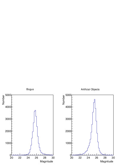
Figure 2: Distribution of magnitudes of bogus objects (left) and artificial “real” objects (right) in the training data made from the May observation.

The small number of real sources, as well as imbalance between the real and bogus, is a major obstacle in effective machine-learning. To improve the performance, we generated artificial transient objects to use as the real sample in training machines.

The procedure is as follows. We constructed spatially-varying PSFs based on the detected stars, using the HSC pipeline, and generated a number of artificial sources from them with different brightness at random positions. Magnitude ($m$) distribution of artificial sources were set to follow $N(m)=10^{0.6m}$, which is expected when the density of sources with the same luminosity is constant in the universe. The faintest magnitude was set at 27.0 mag, and 1,000 artificial sources were generated per CCD chip. These artificial sources were added to the observed images to mimic the actual observing conditions.

We made the training sample containing 33,742 real and 25,468 bogus sources. Figure 2 shows the distribution of magnitudes of bogus and artificial “real” objects. This has made up the number of “real” objects comparable to that of the bogus, and accordingly enabled training with a sufficient number of “real” objects. The data with artificial sources were reduced and features were also extracted in the same manner as for the real sources. Note that this strategy was taken also by Wright et al. (2015).

4.4 Training of Machines

4.4.1 AUC Boosting

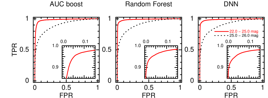
Figure 3: ROC curves of the three machines: AUC Boosting (left), Random Forest (middle), and Deep Neural Network (right), trained with the artificial data, based on the May observation. Horizontal and vertical axes are FPR and TPR, respectively. The red solid and black dotted lines show the curves for the optical magnitude ranges of 22.0–25.0, and 25.0–26.0 mag, respectively. Insets show the magnification of the lines for 22.0–25.0 mag.

In the training step, we first determined the optimal hyper-parameter $\lambda$ by performing cross-validation as follows. We made 30 partitions of randomly sampled data, each of which contained the training, validation and test data with the same size. For each partition of data, we searched for the optimal $\lambda$ parameter, evaluating the performance of the machine with the AUC value for the corresponding validation data. Next, fixing the $\lambda$ parameter to the derived optimal, we trained the machine using the training and validation data, and evaluated the performance with the test data.

Figure 3 (left panel) shows the result: the average of 30 ROC curves of two magnitude slices for the data of May. We obtained the average FPR of 3.0% at the point of the TPR of 90% in the magnitude range of 22.0–25.0 mag.

4.4.2 Random Forest

We determined the meta parameter $B=100$ by the cross-validation in the same way as in the case of AUC boosting (previous subsection). We chose $m_{f}=4$, based on the standard setting for classification task. The ROC curves in the magnitude slices are shown in figure 3 (middle panel). We obtained the average FPR of 0.95% at the point of the TPR of 90% for the same range as in AUC Boosting.

4.4.3 Deep Neural Network

We chose the meta-parameters by preliminary cross validations, as follows. The number of hidden layers was $3$, and thus our DNN was $5$-layered. All emission functions of the hidden units were ReLU (the rectified linear unit). The emission function of the output layer was the soft-max function. We used a classical momentum SGD method to optimize the network with the mini-batch size $M=4000$. The number of maximum iterations was $20000$, but the early stopping rule was employed, following the standard practice of DNNs.

For the cross-validation, we split the sample equally in data size into training, development, and test dataset, keeping the ratio between the real and bogus objects, and prepared $30$ partitions. For each partition, we performed $30$ repetitions of training and evaluation to search for the best combination of meta-parameters of the number of neural units in hidden layers and the step size of SGD, among exhaustive combinations of them. Then, we obtained the average test score of these repetitions.

We obtained the average FPR of 0.85% at the point of the TPR of 90% for the same range as in AUC Boosting. The ROC curves are shown in figure 3 (right panel).

4.5 Combined machine

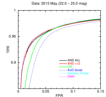
Figure 4: ROC curves of the three ML machines and the combinations of them for the data of 22.0 – 25.0 mag on 2015 May. Those of AUC boosting, RF, and DNN are shown in blue, cyan, and magenta dotted curves, respectively. Those of “unanimous voting”, “majority voting”, and “safeguard minority opinions” are shown in black, red, and green solid curves, respectively.

Finally, we combined the results of the three machines to have a single decision. There are logically three ways to combine three machines indiscriminately (A, B, and C): “unanimous voting”, “majority voting”, and “safeguard minority opinions”, which are basically “A & B & C”, “(A & B) $|$ (B & C) $|$ (C & A)”, and “A $|$ B $|$ C”, respectively, where “&” and “$|$” denote logical “AND” and “OR”, respectively. Figure 4 summarizes their ROC curves, together with the ones with individual machines. We found the FPR of the combined machines at the TPR of 90% to be 1.0%, 1.0%, and 2.1% for the above-mentioned three combinations, respectively. Among them, the performance of “safeguard minority opinions” is not good, whereas the performances of “unanimous voting” and “majority voting” are good. We have decided to use “majority voting”, because the “unanimous voting” would give too tight constraints.

4.6 Robustness for variation of environment

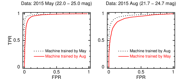
Figure 5: Combined ROC curves as “majority voting” of the three ML machines. Left: ROC curve made by evaluating the data of 22.0 – 25.0 mag on 2015 May, using the machine trained with the same data (black dot) and the data on 2015 Aug (red solid). Right: ROC curve made by evaluating the data of 21.7 – 24.7 mag on 2015 August, using the machine trained with the same data (black dot) and the data on 2015 May (red solid).

To validate that our machines are robust against variations of environment, we made the following ROC curves. Figure 5 (left) shows two ROC curves of the combined “majority voting” machine applied to the artificial data on May; the black dotted curve shows the result of the machine trained with the same data, while the red solid curve is the result of the machine trained with artificial data on August. Figure 5 (right) shows the ROC curves of the data for which May and August are swapped. In both the panels, the red solid curves are slightly worse than the black dotted curves, but the differences are small. We conclude that the machines trained with the adopted method are robust against changes of the conditions.

4.7 Results of selection of supernovae

lr Number of selected objects in the 2015 August data Selection # of objects
Total 45,019
AUC Boosting 21,487
Random Forest 16,307
Deep Neural Network 11,645
Two or three machines 16,888
All machines 8,514

Table 4.7 summarizes the numbers of selected objects obtained with the three individual machines and with the combined machines, where the thresholds are set at the points corresponding to the TPR of 90%. In order not to miss the real objects, we adopted the “majority voting” for the combined machines, and it reduced the number of objects to $16,888$.

Among 48 supernovae obtained with the May observation, 26 are in the magnitude range of 22.0 – 25.0 mag. We applied the combined machine of “majority voting” with the threshold of TPR of 90% at this magnitude range. Then, 22 sources, or 85% of them, were accepted.

4.8 Quick selection of supernovae

Before the August observation, we had installed the trained machines in order to run transient search immediately after the observation (see section 4.7). We then visually inspected every object detected, selected ten clean sources as definite candidates of supernovae, and reported the list to Astronomers’ Telegram (Tominaga et al., 2015c). This whole process was carried out within the same day as the observation.

5 Discussion and Conclusion

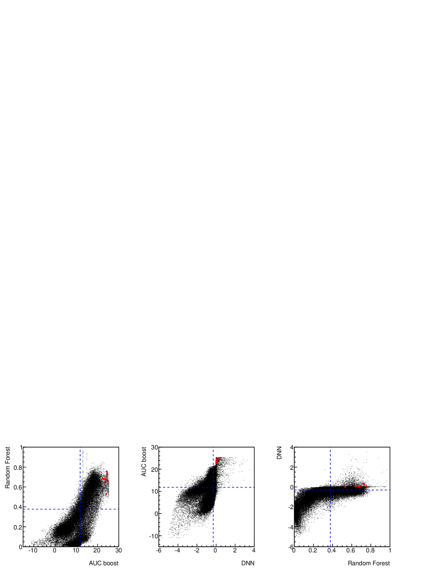
Figure 6: Cross-relations of scores obtained with the three machines for the entire sample (black) and the selected sample of ten candidates of supernovae reported to Astronomers’ Telegram (Tominaga et al., 2015c) (red) for the observation data on 2015 August 19. The left, middle, and right panels plot those of Random Forest v.s. AUC Boosting, AUC Boosting v.s. Deep Neural Network, and Deep Neural Network v.s. Random Forest, respectively. Horizontal and vertical dashed lines show the thresholds corresponding to the TPR of 90%.

We performed Subaru/HSC observations in 2015 May and August, made transient searches, and applied machine-learning techniques to the result to reduce the bogus transient objects. We have developed real-bogus classifiers as the core function for it, using the three machine-learning methods of AUC Boosting, Random Forests, and Deep Neural Network, and then made the combined classifier as their majority voting. We have installed our machines in the analysis pipeline of the HSC, and successfully found real supernovae within the same day as the observation, demonstrating the power of our method. Now, we have completed the preparation for the forthcoming HSC/SSP transient survey observation.

In training our machines, we used artificial objects, because the data are highly imbalanced between real/bogus objects, and it was found to be crucial to make good machines efficiently. Although the HSC survey data are technically more difficult to deal with than other survey data, given that the HSC survey is deeper than other surveys, we have achieved the results comparable to the similar studies in other surveys.

The cross-relations between three machines in figure 6 show that none of the three is significantly better than the other two. Therefore, combining the machines is beneficial. We used a moderate selection with all the combinations of multiple machines, “majority voting”, to avoid missing some real objects. For the machine, robustness against variation of environment was confirmed.

In this paper we have focused on real-bogus separation with machine-learning methods, and have demonstrated that they were indeed useful. Their use in extracting scientific results out of Big-data in astronomy is promising. As the next step, we will use machine-learning for classification of types of transients, by combining timing and color information, as well as the shape of objects.

We thank the Subaru Hyper Suprime-Cam team. This work is supported by Core Research for Evolutionary Science and Technology (CREST), Japan Science and Technology Agency (JST). It is also supported by the research grant program of Toyota foundation (D11-R-0830) and was in part supported by Grants-in-Aid for Scientific Research of JSPS (15H02075), MEXT (15H00788), and the World Premier International Research Center Initiative, MEXT, Japan. This paper makes use of software developed for the LSST. We thank the LSST Project for allowing their code available as free software at http://dm.lsstcorp.org.

References

- Aihara et al. (2011) Aihara, H., et al. 2011, ApJS, 193, 29
- Alard (2000) Alard, C. 2000, A&AS, 144, 363
- Alard & Lupton (1998) Alard, C., & Lupton, R. H. 1998, ApJ, 503, 325
- Axelrod et al. (2010) Axelrod, T. et al. 2010, in SPIE Conference Series, Vol. 7740, SPIE Conference Series, 15
- Bailey et al. (2007) Bailey, S. et al., 2007, ApJ, 665, 1246
- Bertin & Arnouts (1996) Bertin, E., & Arnouts, S. 1996, A&AS, 117, 393
- Bloom et al. (2012) Bloom, J. S. et al., 2012, PASP, 124, 1175
- Breiman (2001) Breiman, L., 2001, Machine Learning, 45, 5
- Brink et al. (2013) Brink, H., et al., 2013, MNRAS, 435, 1047
- Dahl (2012) Dahl, G. E., Yu, D., Deng, Li., & Acero, A., 2012, IEEE Transactions on Audio, Speech and Language Processing, 20, 30
- du Buisson et al. (2015) du Buisson, L., et al. 2015, MNRAS, 454, 2026
- Goldstein et al. (2015) Goldstein, D. A., et al., 2015, AJ, 150, 82
- Rosenblatt (1958) Frank, R., 1958, Psychological Review, 65, 386
- Furusawa et al. (2011) Furusawa, H., et al., 2011, PASJ, 63, 585
- Hastie, Tibshirani & Friedman (2009) Hastie, T., Tibshirani, R. & Friedman, J. 2009, “The Elements of Statistical Learning”, 2nd. Edition, Springer.
- Ivezic et al. (2008) Ivezic, Z., et al., 2008, arXiv:0805.2366
- Komori (2011) Komori, O. 2011, Ann. Inst. Stat. Math, 63, 961
- Krizhevsky (2012) Krizhevsky, A., Sutskever, I., & Hinton, G. E., 2012, Advances in Neural Information Processing Systems (Proceedings of NIPS), 25, 1
- LeCun (2015) LeCun, Y., Bengio, Y., & Hinton, G., 2015, Nature, 521, 436
- McCulloch & Pitts (1943) McCulloch, W. S. & Pitts, W., 1943, The Bulletin of Mathematical Biophysics, 5, 115
- Miyazaki et al. (2012) Miyazaki, S., et al., 2012, SPIE Proc., 8446, 84460Z
- Morokuma et al. (2016) Morokuma, T., et al., 2016, PASJ, 68, 40
- Tanaka et al. (2016) Tanaka, M., et al., 2016, ApJ, 819, 5
- Tominaga et al. (2015a) Tominaga, N., et al., 2015a, submitted to ApJ
- Tominaga et al. (2015b) Tominaga, N., et al., 2015b, The Astronomer’s Telegram, 7565
- Tominaga et al. (2015c) Tominaga, N., et al., 2015c, The Astronomer’s Telegram, 7927
- Wright et al. (2015) Wright, D. E. et al. 2015, MNRAS, 449, 451