Critical noise of majority-vote model on complex networks

Abstract

The majority-vote model with noise is one of the simplest nonequilibrium statistical model that has been extensively studied in the context of complex networks. However, the relationship between the critical noise where the order-disorder phase transition takes place and the topology of the underlying networks is still lacking. In the paper, we use the heterogeneous mean-field theory to derive the rate equation for governing the model’s dynamics that can analytically determine the critical noise $f_{c}$ in the limit of infinite network size $N\rightarrow\infty$. The result shows that $f_{c}$ depends on the ratio of ${\left\langle k\right\rangle}$ to ${\left\langle{{k^{{3\mathord{\left/{\vphantom{32}}\right.\kern-1.2pt}2}}}}\right\rangle}$, where ${\left\langle k\right\rangle}$ and ${\left\langle{{k^{{3\mathord{\left/{\vphantom{32}}\right.\kern-1.2pt}2}}}}\right\rangle}$ are the average degree and the ${{3\mathord{\left/{\vphantom{32}}\right.\kern-1.2pt}2}}$ order moment of degree distribution, respectively. Furthermore, we consider the finite size effect where the stochastic fluctuation should be involved. To the end, we derive the Langevin equation and obtain the potential of the corresponding Fokker-Planck equation. This allows us to calculate the effective critical noise $f_{c}(N)$ at which the susceptibility is maximal in finite size networks. We find that the $f_{c}-f_{c}(N)$ decays with $N$ in a power-law way and vanishes for $N\rightarrow\infty$. All the theoretical results are confirmed by performing the extensive Monte Carlo simulations in random $k$-regular networks, Erdös-Rényi random networks and scale-free networks.

I Introduction

Equilibrium and nonequilibrium phase transitions in ensembles of complex networked systems have been a subject of intense research in the field of statistical physics and many other disciplines Boccaletti et al. (2006); Arenas et al. (2008); Dorogovtsev et al. (2008); Boccaletti et al. (2014). Owing to the inherent randomness and heterogeneity in the interacting patterns, phase transitions on complex networks are drastically different from those on regular lattices in Euclidean space. Examples range from the anomalous behavior of Ising model Aleksiejuk et al. (2002); Bianconi (2002); Dorogovtsev et al. (2002); Leone et al. (2002); Bradde et al. (2010) to a vanishing percolation threshold Cohen et al. (2000); Callaway et al. (2000) and the absence of epidemic thresholds that separate healthy and endemic phases Pastor-Satorras and Vespignani (2001); Boguñá et al. (2003, 2013) as well as explosive emergence of phase transitions Achlioptas et al. (2009); Friedman and Landsberg (2009); Radicchi and Fortunato (2009); Cho et al. (2009); da Costa et al. (2010); Grassberger et al. (2011); Riordan and Warnke (2011); Buldyrev et al. (2010); Parshani et al. (2010); Gao et al. (2011); Gómez-Gardeñes et al. (2011); Leyva et al. (2012); Majdandzic et al. (2014). So far, unveiling the relationship between the onset of phase transitions and the topology of the underlying networks is still a topic of considerable attention.

The majority-voter (MV) model is a simple nonequilibrium Ising-like system with up-down symmetry that presents an order-disorder phase transition at a critical value of noise Castellano et al. (2009). Since Oliveira pointed out that the MV model on a square lattice belongs to the universality class of the equilibrium Ising model de Oliveira (1992), the model has been extensively studied in the context of complex networks, including random graphs Pereira and Moreira (2005); Lima et al. (2008), small world networks Campos et al. (2003); Luz and Lima (2007); Stone and McKay (2015), scale-free networks Lima (2006); Lima and Malarz (2006), and some others Kwak et al. (2007); Yang et al. (2008); Wu and Holme (2010); Santos et al. (2011); Acuña Lara and Sastre (2012); Acuña Lara et al. (2014). These results showed that the critical exponents are generally dependent on the underlying interacting substrates. However, the studies of pervious works are mainly based on numerical simulations. Especially, the analytical determination of the critical noise is still lacking at present.

For this purpose, in this paper we employ the heterogeneous mean-field theory to derive the rate equation for governing the MV model’s dynamics on undirected networks. According to linear stability analysis, we determine the critical point of noise $f_{c}$, the onset of an order-disorder phase transition in the limit of infinite size networks $N\rightarrow\infty$. The analytical result shows that $f_{c}$ is related to the ratio of the first moment to the ${3\mathord{\left/{\vphantom{32}}\right.\kern-1.2pt}2}$ order moment of degree distribution. Furthermore, we derive the Langevin equation to study the effect of stochastic fluctuation on finite size networks. By solving the potential of the corresponding Fokker-Planck equation, we calculate the susceptibility as a function of noise and determine the effective critical noise $f_{c}(N)$ on finite size networks at which the susceptibility is maximal. We find that the difference $f_{c}-f_{c}(N)$ decays in power-law ways with $N$. Extensive Monte Carlo (MC) simulations are performed on diverse network types to validate the theoretical results.

II Model

We consider the MV model with noise on complex networks defined by a set of spin variables $\{\sigma_{i}\}$ $(i=1,\ldots,N)$, where each spin is associated to one node of the underlying network and can take the values $\pm 1$. The system evolves as follows: for each spin $i$, we first determine the majority spin of $i^{\prime}$s neighborhood. With probability $f$ the node $i$ takes the opposite sign of the majority spin, otherwise it takes the same spin as the majority spin. The probability $f$ is called the noise parameter and plays a similar role of temperature in equilibrium spin systems. In this way, the single spin flip probability can be written as

$$w({\sigma_{i}})=\frac{1}{2}\left[{1-\left({1-2f}\right){\sigma_{i}}S\left({\sum\limits_{j}{{a_{ij}}{\sigma_{j}}}}\right)}\right],$$ (1)

where $S(x)=sgn(x)$ if $x\neq 0$ and $S(0)=0$. In the latter case the spin $\sigma_{i}$ is flipped to $\pm 1$ with probability equal to ${1\mathord{\left/{\vphantom{12}}\right.\kern-1.2pt}2}$. The elements of the adjacency matrix of the underlying network are defined as $a_{ij}=1$ if nodes $i$ and $j$ are connected and $a_{ij}=0$ otherwise. In the case $f=0$, the majority-vote model is identical to the zero temperature Ising model Zhou and Lipowsky (2005); Castellano and Pastor-Satorras (2006).

III Results

To proceed a mean-field treatment, we first define $q_{k}$ as the probability that a node of degree $k$ is in $+1$ state, and $Q$ as the probability that for any node in the network, a randomly chosen nearest neighbor node is in $+1$ state. Furthermore, for any node the probability that a randomly chosen nearest neighbor node has degree $k$ is ${{kP(k)}\mathord{\left/{\vphantom{{kP(k)}{\left\langle k\right\rangle}}}\right.\kern-1.2pt}{\left\langle k\right\rangle}}$, where $P(k)$ is degree distribution defined as the probability that a node chosen at random has degree $k$ and $\left\langle k\right\rangle$ is the average degree Dorogovtsev et al. (2008). It is supposed to be reasonable only in networks without degree correlation. The probabilities $q_{k}$ and $Q$ satisfy the relation

$$Q=\sum\limits_{k}{kP(k)}{{{q_{k}}}\mathord{\left/{\vphantom{{{q_{k}}}{\left\langle k\right\rangle}}}\right.\kern-1.2pt}{\left\langle k\right\rangle}}.$$ (2)

Thus, we can write rate equations for $q_{k}$ as

$${{\dot{q}}_{k}} = -{q_{k}}(1-{\psi_{k}})+(1-{q_{k}}){\psi_{k}}$$ (3)

$$= -{q_{k}}+{\psi_{k}},$$

where ${\psi_{k}}$ is is the probability that a node of degree $k$ takes the $+1$ value, which can be expressed as

$${\psi_{k}(Q)}=(1-f){\varphi_{k}}(Q)+f({1-\varphi_{k}}(Q)).$$ (4)

Here, ${\varphi_{k}}(Q)$ is the probability that a node of degree $k$ with $+1$ state takes the majority rule, which can be written by a binomial distribution,

$${\varphi_{k}}(Q)=\sum\limits_{n=\left\lceil{k/2}\right\rceil}^{k}{\left(1-\frac{1}{2}{\delta_{n,k/2}}\right)C_{k}^{n}}{Q^{n}}{(1-Q)^{k-n}},$$ (5)

where $\left\lceil\cdot\right\rceil$ is the ceiling function, $\delta$ is the Kronecker symbol, and $C_{k}^{n}={{k!}\mathord{\left/{\vphantom{{k!}{[n!(k-n)!])}}}\right.\kern-1.2pt}{[n!(k-n)!]}}$ are the binomial coefficients. By introducing Eq.(3) into Eq.(2) we obtain a closed rate equation for the quantity $Q$,

$$\dot{Q}=-Q+\Psi(Q),$$ (6)

where

$$\Psi(Q)=\sum\limits_{k}{kP(k)}{{{\psi_{k}}(Q)}\mathord{\left/{\vphantom{{{\psi_{k}}(Q)}{\left\langle k\right\rangle}}}\right.\kern-1.2pt}{\left\langle k\right\rangle}}.$$ (7)

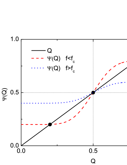
Figure 1: (color online). Graphic demonstration of steady state solutions of $Q$. When $f$ is less than a critical value $f_{c}$, there are three solutions. One is at $Q=\frac{1}{2}$ corresponding to a disordered phase and the other two correspond to two symmetric ordered phases. For $f>f_{c}$ , there is only one solution at $Q=\frac{1}{2}$.

In the steady state $\dot{Q}=0$, we have $Q_{s}=\Psi(Q_{s})$. Fig.1 shows that the two typical examples of graphic solutions of $Q_{s}$. One can easily find that a trivial stationary solution, $Q_{s}=\frac{1}{2}$, always exists irrespective of the value of $f$ (corresponding to a disordered phase $\left\langle{{\sigma_{i}}}\right\rangle=0$), as ${\varphi_{k}}(\frac{1}{2})=\frac{1}{2}$ and ${\Psi}(\frac{1}{2})=\frac{1}{2}$. However, the other two solutions are possible if $f$ is less than a critical value $f_{c}$, and they represent the existence of two ordered phases with up-down symmetry. Therefore, the critical noise $f_{c}$ is determined by the condition that the derivation of $\Psi(Q)$ with $Q$ equals to one at $f=f_{c}$, i.e.,

$${\left.{\frac{{d\Psi(Q)}}{{dQ}}}\right|_{Q=\frac{1}{2}}}=1.$$ (8)

To do this, we rewrite approximately Eq.(5) as

$${\varphi_{k}}(Q)={\varphi_{k}}(\frac{1}{2}+y)=\frac{1}{2}+\frac{1}{2}erf\left({y\sqrt{2k}}\right),$$ (9)

where $erf(x)$ is the error function. Note that this approximation is plausible for large values of $k$ as the binomial distribution can be approximated by a normal distribution and the sum over $n$ in Eq.(5) can be substituted by an integral Castellano and Pastor-Satorras (2006). The derivation of $\Psi(Q)$ with $Q$ can be expressed analytically by

$${\left.{\frac{{d\Psi(Q)}}{{dQ}}}\right|_{Q=\frac{1}{2}}} = {\left.{\sum\limits_{k}{\frac{{kP(k)}}{{\left\langle k\right\rangle}}(1-2f)}\frac{{d\varphi(\frac{1}{2}+y)}}{{dy}}}\right|_{y=0}}$$ (10)

$$= {\left.{\sum\limits_{k}{\frac{{kP(k)}}{{\left\langle k\right\rangle}}(1-2f)}\sqrt{\frac{{2k}}{\pi}}{e^{-2k{y^{2}}}}}\right|_{y=0}}$$

$$= (1-2f)\sqrt{\frac{2}{\pi}}\frac{{\left\langle{{k^{{3\mathord{\left/{\vphantom{32}}\right.\kern-1.2pt}2}}}}\right\rangle}}{{\left\langle k\right\rangle}},$$

where $\left\langle{{k^{n}}}\right\rangle=\sum\nolimits_{k}{{k^{n}}P(k)}$ is the $n$th moment of degree distribution. Inserting Eq.(10) into Eq.(8), we arrive at the analytical expression of $f_{c}$,

$${f_{c}}=\frac{1}{2}-\frac{1}{2}\sqrt{\frac{\pi}{2}}\frac{{\left\langle k\right\rangle}}{{\left\langle{{k^{{3\mathord{\left/{\vphantom{32}}\right.\kern-1.2pt}2}}}}\right\rangle}}.$$ (11)

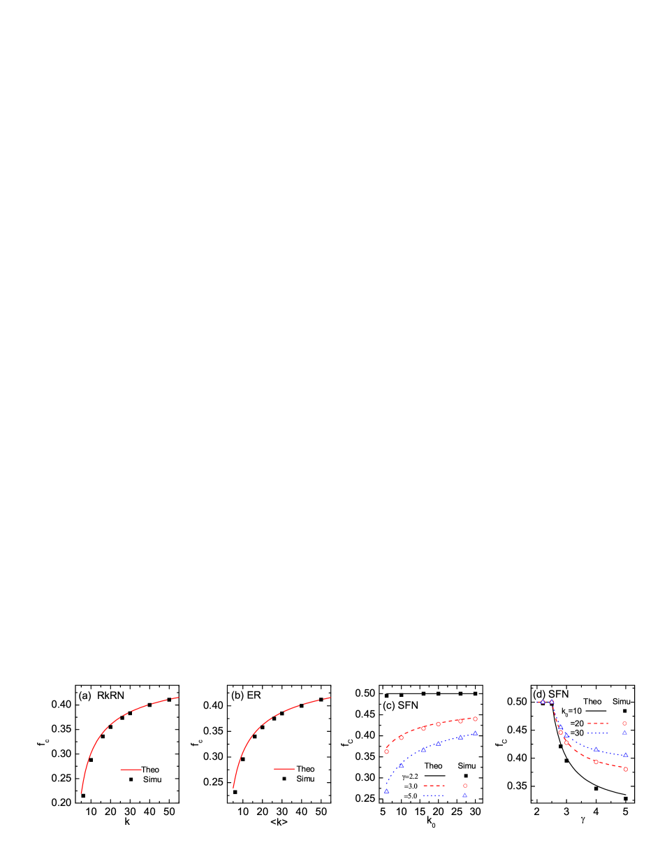
Figure 2: (color online). The critical noise $f_{c}$ obtained from the theory (lines) and MC simulation (symbols) on (a) RkRN, (b) ERRN, and (b-c) SFN.

To validate the theoretical results on $f_{c}$, we shall consider the three network types: the random $k$-regular networks (RkRN) and Erdös-Rényi random networks (ERRN), as the representations of degree homogeneous networks, and scale-free networks (SFN) as the representations of degree heterogeneous networks. For RkRN, each node has the same degree $k$ and degree distribution follows the delta-like function $P(k)=\delta(k)$, and thus Eq.(11) can be reduced to

$$f_{c}^{RkRN}=\frac{1}{2}-\frac{1}{2}\sqrt{\frac{\pi}{2}}\frac{1}{{\sqrt{k}}}.$$ (12)

From Eq.(12), we see that $f_{c}$ is a decreasing function of $k$. For $k=N-1\rightarrow\infty$, $f_{c}=\frac{1}{2}$ and RkRN thus become the globally connected networks. For ERRN, degree distribution follows Poisson $P(k)={\left\langle k\right\rangle^{k}}{{{e^{-\left\langle k\right\rangle}}}\mathord{\left/{\vphantom{{{e^{-\left\langle k\right\rangle}}}{k!}}}\right.\kern-1.2pt}{k!}}$ with the average degree $\left\langle k\right\rangle$, and the theoretical value of $f_{c}$ for ERRN can be numerically calculated according to Eq.(11).

For SFN, degree distribution follows a pow-law function $P(k)\sim{k^{-\gamma}}$, with degree exponent $\gamma>2$. In the thermodynamic limit $N\to\infty$, ${\left\langle{{k^{{3\mathord{\left/{\vphantom{32}}\right.\kern-1.2pt}2}}}}\right\rangle}$ diverges for $\gamma\leq{5\mathord{\left/{\vphantom{52}}\right.\kern-1.2pt}2}$, such that the critical noise becomes $f_{c}=\frac{1}{2}{\kern 1.0pt}{\kern 1.0pt}$ according to Eq.(11). For $\gamma>{5\mathord{\left/{\vphantom{52}}\right.\kern-1.2pt}2}$, both $\left\langle k\right\rangle$ and ${\left\langle{{k^{{3\mathord{\left/{\vphantom{32}}\right.\kern-1.2pt}2}}}}\right\rangle}$ are finite in the limit of $N\to\infty$, and they are $\gamma-$dependent given by $\left\langle k\right\rangle={{(\gamma-1){k_{0}}}\mathord{\left/{\vphantom{{(\gamma-1){k_{0}}}{(\gamma-2}}}\right.\kern-1.2pt}{(\gamma-2}}{\kern 1.0pt})$ and $\left\langle{{k^{{3\mathord{\left/{\vphantom{32}}\right.\kern-1.2pt}2}}}}\right\rangle={{(\gamma-1)k_{0}^{{3\mathord{\left/{\vphantom{32}}\right.\kern-1.2pt}2}}}\mathord{\left/{\vphantom{{(\gamma-1)k_{0}^{1.5}}{(\gamma-2.5}}}\right.\kern-1.2pt}{(\gamma-{5\mathord{\left/{\vphantom{32}}\right.\kern-1.2pt}2}}}{\kern 1.0pt})$ with $k_{0}$ being the minimal node degree. By the above analysis, we immediately obtain the critical noise $f_{c}$ for SFN

$$f_{c}^{SFN}=\left\{\begin{aligned} &\frac{1}{2}-\frac{1}{2}\sqrt{\frac{\pi}{2}}\frac{{\gamma-{5\mathord{\left/{\vphantom{52}}\right.\kern-1.2pt}2}}}{{\gamma-2}}\frac{{1{\kern 1.0pt}{\kern 1.0pt}{\kern 1.0pt}{\kern 1.0pt}}}{{\sqrt{{k_{0}}}}},&\gamma>{5\mathord{\left/{\vphantom{52}}\right.\kern-1.2pt}2}{\kern 1.0pt}{\kern 1.0pt}\\ &\frac{1}{2},&\gamma\leq{5\mathord{\left/{\vphantom{52}}\right.\kern-1.2pt}2}\end{aligned}\right.$$ (13)

We firstly generate the networks according to the Molloy-Reed model Molloy and Reed (1995): each node is assigned a random number of stubs $k$ that is drawn from a given degree distribution. Pairs of unlinked stubs are then randomly joined. We then run the standard MC simulation: at each MC step, each node is firstly randomly chosen once on average and then make an attempt to flip spin with the probability according to Eq.(1).

In order to numerically obtain the $f_{c}$, we need to calculate the Binder’s fourth-order cumulant $U$, defined as

$$U=1-\frac{{\left[{\left\langle{{m^{4}}}\right\rangle}\right]}}{{3{{\left[{\left\langle{{m^{2}}}\right\rangle}\right]}^{2}}}},$$ (14)

where $m={{\sum\nolimits_{i=1}^{N}{{\sigma_{i}}}}\mathord{\left/{\vphantom{{\sum\nolimits_{i=1}^{N}{{\sigma_{i}}}}N}}\right.\kern-1.2pt}N}$ is the average magnetization per node, $\left\langle\cdot\right\rangle$ denotes time averages taken in the stationary regime, and $\left[\cdot\right]$ stands for the averages over different network configurations. The critical noise $f_{c}$ is estimated as the point where the curves $U\sim f$ for different network sizes $N$ intercept each other. In our simulations, $f_{c}$ is determined by five different network sizes: $N=500$, $1000$, $2000$, $5000$ and $10000$.

For comparison, in Fig.2 we plot the $f_{c}$ obtained from the theoretical prediction (lines) and the MC simulation (symbols), respectively. In Fig.2(a) and Fig.2(b), we show the results on RkRN and on ERRN, respectively. In Fig.2(c-d), we show the results on SFN and plot the $f_{c}$ as a function of $k_{0}$ for some fixed $\gamma$ in Fig.2(c) and of $\gamma$ for some fixed $k_{0}$ in Fig.2(d). It is clearly observed that for large values $k$ there are an excellent agreements between the theory and simulation. However, for relatively small $k$ the used approximation in Eq.(9) is not very valid, such that the discrepancy between them exists.

So far, we have obtained the analytical expression of $f_{c}$ and confirmed its validity by performing MC simulations on different networks. The expression is only valid for infinite size networks $N\rightarrow\infty$ where the finite-size fluctuation is ignored. For finite size networks, the fluctuation is unavoidable and the actual phase transition never happens. However, one can define an effective critical noise $f_{c}(N)$ at which the susceptibility (the variance of an order parameter) is maximal. Obviously, $f_{c}(N)$ is size-dependent and recovers $f_{c}$ in the limit of $N\rightarrow\infty$. To get $f_{c}(N)$, we will derive the fluctuation-driven Langevin equation for $Q$ Boguñá et al. (2009); Caccioli and Dall’Asta (2009):

$$\dot{Q}=\mathbb{E}[\Delta Q]+\sqrt{\mathbb{V}[\Delta Q]}\xi(t)$$ (15)

where $\mathbb{E}[\Delta Q]$ and $\mathbb{V}[\Delta Q]$ are the mean value and the variance of the variation of $Q$, respectively, and $\xi(t)$ is a Gaussian white noise satisfying $\left\langle{\xi(t)}\right\rangle=0$ and $\left\langle{\xi(t)\xi(t^{\prime})}\right\rangle=\delta(t-t^{\prime})$. For the present model, $\mathbb{E}[\Delta Q]$ and $\mathbb{V}[\Delta Q]$ can be computed as

$$\mathbb{E}[\Delta Q] = N\sum\limits_{k}{P(k){q_{k}}[1-{\psi_{k}}(Q)]\left({-{k\over{N\left\langle k\right\rangle}}}\right)}$$ (16)

$$+N\sum\limits_{k}{P(k)(1-{q_{k}}){\psi_{k}}(Q)\left({{k\over{N\left\langle k\right\rangle}}}\right)}$$

$$= -Q+\Psi(Q),$$

and

$$\mathbb{V}[\Delta Q] = N\sum\limits_{k}{P(k){q_{k}}[1-{\psi_{k}}(Q)]}{\left({-{k\over{N\left\langle k\right\rangle}}}\right)^{2}}$$

$$+N\sum\limits_{k}{P(k)(1-{q_{k}}){\psi_{k}}(Q){{\left({{k\over{N\left\langle k\right\rangle}}}\right)}^{2}}}$$

$$= \sum\limits_{k}{{{{k^{2}}P(k)}\over{N{{\left\langle k\right\rangle}^{2}}}}}\left[{q{{}_{k}}(1-{\psi_{k}}(Q))+(1-{q_{k}}){\psi_{k}}(Q)}\right]$$

Equation (LABEL:eq17) is not yet a closed equation for $Q$ because the diffusion term $\mathbb{V}[\Delta Q]$ involve degree-dependent quantities $q_{k}$. To close it, we use the quasi-static approximation obtained from the rate equations (3) imposing $\dot{q}_{k}\simeq 0$, i.e., $q_{k}\simeq\psi_{k}(Q)$ Boguñá et al. (2009); Caccioli and Dall’Asta (2009). The approximation assumes that $Q(t)$ varies much slowly with respect to the dynamics of the microscopic degrees of freedom $q_{k}(t)$. By the approximation, Eq.(17) becomes

$$\mathbb{V}[\Delta Q]={2\over{N{{\left\langle k\right\rangle}^{2}}}}\sum\limits_{k}{{k^{2}}P(k)}{\psi_{k}}(Q)(1-{\psi_{k}}(Q))$$ (18)

Therefore, we obtain the fluctuation-driven Langevin equation with a closed form,

$$\dot{Q}=-Q+\Psi(Q)+\sqrt{2D(Q)}\xi(t)$$ (19)

with multiplicative noise $D(Q)={1\over{N{{\left\langle k\right\rangle}^{2}}}}\sum\nolimits_{k}{{k^{2}}P(k)}{\psi_{k}}(Q)(1-{\psi_{k}}(Q))$. Clearly, in the limit of $N\rightarrow\infty$, the fluctuation term $D(Q)\rightarrow 0$, and Eq.(19) thus recovers to the mean-field equation derived in Eq.(6).

Furthermore, let $P(Q,t)$ denote the probability density distribution of $Q$ at time $t$. Then, the Fokker-Planck equation of $P(Q,t)$ corresponding to Eq.(19) can be given by

$$\frac{{\partial P(Q,t)}}{{\partial t}}= - \frac{\partial}{{\partial Q}}\left[{-Q+\Psi(Q)+\sqrt{D(Q)D^{\prime}(Q)}}\right]P(Q,t)$$ (20)

$$+ \frac{{{\partial^{2}}}}{{{\partial^{2}}Q}}{D(Q)}P(Q,t)$$

The stationary distribution is $P(Q)=Ce^{U_{FP}(Q)}$ where $C$ is the normalized constant and

$${U_{FP}}(Q)=\frac{1}{2}\ln\left[{D(Q)}\right]-\int^{Q}{\frac{{-S+\Psi(S)}}{{D(S)}}}dS$$ (21)

is called the potential of the Fokker-Planck equation Risken (1992).

The critical noise $f_{c}(N)$ for finite size networks is determined using the modified susceptibility $\chi^{\prime}$ defined as

$$\chi^{\prime}=N\left[{\left\langle{{y^{2}}}\right\rangle-{{\left\langle|y|\right\rangle}^{2}}}\right],$$ (22)

where $y=Q-\frac{1}{2}$, $\left\langle{{|y|}}\right\rangle$ and $\left\langle{{y^{2}}}\right\rangle$ are calculated by the integrals

$$\left\langle{\left|y\right|}\right\rangle=\int_{0}^{1}{\left|{Q-\frac{1}{2}}\right|P(Q)dQ}$$ (23)

and

$$\left\langle{{y^{2}}}\right\rangle=\int_{0}^{1}{{{\left({Q-\frac{1}{2}}\right)}^{2}}P(Q)dQ},$$ (24)

respectively. We expect that $\chi^{\prime}$ have a peak at $f=f_{c}(N)$ that diverges and $f_{c}(N)$ converges to $f_{c}$ when the network size increases.

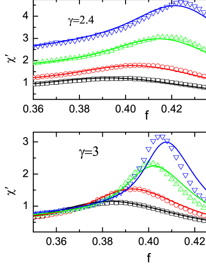
Figure 3: (color online). The susceptibility $\chi^{\prime}$ as a function of noise $f$ for some different network sizes: $N=1000,2000,5000,10000$. (a) RkRN: $k=20$, (b) ERRN: $\left\langle k\right\rangle=20$, (c) SFN: $\gamma=2.4$ and $k_{0}=20$, and (d) $\gamma=3$ and $k_{0}=20$. Lines and symbols indicate the results from theory and MC simulation, respectively.

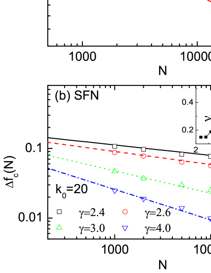
Figure 4: (color online). Log-log plot of the differences of the effective critical noise $f_{c}$ for finite size networks with $f_{c}$, $\Delta f(N)={f_{c}}-{f_{c}}(N)$, with $N$ on (a) RkRN: $k=20$, ERRN: $\left\langle k\right\rangle=20$, and (b) SFN: $k_{0}=20$. $\Delta f(N)$ power law decays with $N$: $\Delta f(N)\sim{N^{-\nu}}$. Lines and symbols indicate the results from theory and MC simulation, respectively. The inset of Fig.4(b) shows the exponent $\nu$ as a function of $\gamma$.

In Fig.3, we show that $\chi^{\prime}$ as a function of noise $f$ for some different network sizes $N$ on RkRN, ERRN, and SFN. For comparison, the values of $\chi^{\prime}$ obtained from the theoretical calculations for Eq.(22) and from MC simulations are indicated by the lines and symbols, respectively. The theoretical calculations can give a well prediction for simulation results. As mentioned above, the point corresponding to the maximal $\chi^{\prime}$ lies in the effective critical noise $f_{c}(N)$ for finite size networks. In addition, we should note that we find that from MC simulations the commonly used susceptibility $\chi=N\left[{\left\langle{{m^{2}}}\right\rangle-{{\left\langle|m|\right\rangle}^{2}}}\right]$ and our used susceptibility $\chi^{\prime}$ defined in Eq.(22) share the same locations where they are maximal (results not shown here).

In Fig.4, we plot the difference $\Delta f(N)={f_{c}}-{f_{c}}(N)$ as a function of $N$ in double logarithm coordinates. The lines and symbols also indicate the results of theoretical calculations from Eq.(22) and MC simulations, respectively. As pointed out by many previous studies, $\Delta f(N)$ scale with $N$ in a power-law way: $\Delta f(N)\sim{N^{-\nu}}$. With the increment of $N$, $\Delta f(N)$ decreases and tends to zero in the limit $N\rightarrow\infty$, recovering the result of Eq.(11). For RkRN and ERRN, we find that the exponents $\nu$ are independent of $k$ and $\left\langle k\right\rangle$. For SFN, $\nu$ is also almost independent of $k_{0}$ but is an increasing function of $\gamma$ (see the inset of Fig.4(b)).

IV Conclusions

In conclusion, we have used heterogeneous mean-field theory to derive the rate equation of an order parameter $Q$ for the MV model defined on complex networks. By the linear stability analysis, we have analytically obtained the critical noise $f_{c}$ at which the order-disorder phase transition takes place in the limit of infinite size networks. We find that that $f_{c}$ is determined by both the first and ${3\mathord{\left/{\vphantom{32}}\right.\kern-1.2pt}2}$ order moments of degree distribution of the underlying networks. Moreover, we have incorporated the effect of stochastic fluctuation on finite size networks via the derivation of the Langevin equation of $Q$. By solving the corresponding Fokker-Planck equation, we have obtained the effective critical noise $f_{c}(N)$ where the susceptibility is maximal. The results show that $f_{c}-f_{c}(N)$ power law decreases with $N$ and reduces to zero in the limit of $N\rightarrow\infty$. To validate the theoretical results, we have performed the extensive MC simulations on RkRN, ERRN, and SFN. There are excellent agreement between the theory and simulations. However, our theory does not perform well on very sparse networks. Therefore, in the future it will be desirable to develop high order theories (such as pair approximation Eames and Keeling (2002); Pugliese and Castellano (2009); Mata et al. (2014); Gleeson (2011)) to obtain more accurate estimation of the critical point of the networked MV model.