Postprocessing for Iterative Differentially Private Algorithms

Abstract

Iterative algorithms for differential privacy run for a fixed number of iterations, where each iteration learns some information from data and produces an intermediate output. However, the algorithm only releases the output of the last iteration, and from which the accuracy of algorithm is judged. In this paper, we propose a post-processing algorithm that seeks to improve the accuracy by incorporating the knowledge on the data contained in intermediate outputs.

1 Introduction

When designing an iterative algorithm for differential privacy, fully utilizing the information privately learned from data is crucial to the success. Suppose we have a simple algorithm $\mathcal{A}$ that calls the function $\mathcal{K}(D,\theta_{t-1})$ $T$ times in a loop and returns $\theta_{T}$ as the final output, where $D\in\mathcal{X}^{N}$ is the input dataset and $\theta_{t}=\mathcal{K}(D,\theta_{t-1})$ is an intermediate output at the $t$${}^{\textrm{th}}$ iteration. A large class of machine learning algorithms, including clustering, classification, and regression, can be written in this form, where $\mathcal{K}(D,\theta_{t})$ minimizes some objective function and returns $\theta_{t+1}$. By the composition theorem (Dwork & Roth, 2014), if the function $\mathcal{K}$ satisfies $\frac{\epsilon}{T}$-differential privacy, the algorithm $\mathcal{A}$ becomes $\epsilon$-differentially private. At each iteration $t$, the algorithm extracts some information $\theta_{t}$ from the given dataset $D$ using the privacy budget of ${}^{\epsilon}\!\!/\!_{T}$, but it only releases the final output $\theta_{T}$ (thus, the accuracy of the algorithm is largely dependent on the magnitude of noise at the final iteration).

In this paper, we ask the following question: “Can we improve the accuracy of the final output $\theta_{T}$ by incorporating the knowledge contained in the intermediate outputs $\theta_{1},\ldots,\theta_{T-1}$?” Recent studies have shown that post-processing algorithms that make inferences on the original data from noisy outputs can significantly improve the accuracy of the results (Lee et al., 2015; Hay et al., 2010; Lin & Kifer, 2013). The main source of improvements comes from enforcing consistency constraints, a set of (hard) syntactic conditions that hold true for the original data. Inspired by these post-processing algorithms, we view the intermediate outputs $\theta_{1},\ldots,\theta_{T-1}$ as soft constraints on our estimates (i.e., the original data). Note that the privacy guarantee of $\mathcal{A}$ is not degraded by this post-processing. as long as it doesn’t rely on the randomness of $\mathcal{A}$.

Consider a differentially private algorithm $\mathcal{A}$ that generates a sequence of noisy statistics $\{\tilde{\theta}_{1},\ldots,\tilde{\theta}_{T}\}$ such that $\tilde{\theta}_{t}=\mathcal{K}(D,\tilde{\theta}_{t-1})+Y$, where $Y$ is a random variable representing the noise added for privacy. Our goal is to estimate a dataset $\widehat{D}$ from which $\tilde{\theta}_{1},\ldots,\tilde{\theta}_{T}$ are most likely to be generated. Once we have estimated $\widehat{D}$, a new estimator $\hat{\theta}$ can be obtained by repeatedly running $\mathcal{K}$ on $\widehat{D}$ without noise (contrast this to $\tilde{\theta}_{T}$ produced with noise and using fixed number of iterations). Informally, we try to find $\widehat{D}$ such that $\mathcal{K}(D,\tilde{\theta}_{t})\approx\mathcal{K}(\widehat{D},\tilde{\theta}_{t})$ for $t=1,\ldots,T$. We note that the size of $\widehat{D}$ could be different from that of the original dataset, $N$; we only require intermediate outputs of $\mathcal{K}$ on both datasets are similar. However, it is still challenging to efficiently explore the space of all possible datasets. To this end, we propose to use MCMC method with carefully designed proposal distribution. The proposed algorithm builds a Markov chain over the space of all possible datasets and makes use of noisy statistics to efficiently propose the next state. Given a dataset $D_{t}$, the proposed algorithm samples a new dataset $D^{\prime}$ and determines whether to accept or reject the dataset by considering the ratio of $\mathbb{P}(\tilde{\theta}_{1}\ldots,\tilde{\theta}_{T}\mathrel{}\mid\mathrel{}D^{\prime})$ to $\mathbb{P}(\tilde{\theta}_{1},\ldots,\tilde{\theta}_{T}\mathrel{}\mid\mathrel{}D_{t})$, i.e., Metroplis-Hastings step. While doing so, it keeps track of the best scoring dataset.

In this paper, we instantiate this post-processing algorithm in the context of $K$-means clustering. The contributions of this paper are as follows:

• We propose a general framework for post-processing a sequence of noisy private outputs, which improves the accuracy by incorporating intermediate results into the process.

• We applied our framework to $K$-means clustering problem and introduce an efficient proposal distribution that yields low rejection rate.

• Extensive empirical evaluations on both synthetic and real datasets are provided to validate our proposed approach.

2 Related Works

We discuss differentially private algorithms that can be applied to the $K$-means problem. The first algorithm is DP-KMEANS introduced in (Blum et al., 2005; McSherry, 2009). Each step of the algorithm is descripbed in Algorithm 1.

Algorithm 1 DP-KMEANS algorithm

  Input: data $D$, # of clusters $K$, # of iterations $T$

  Initialize $\bm{\mathrm{c}}_{1}^{(0)},\cdots,\bm{\mathrm{c}}_{K}^{(0)}$

  for $t=1$ to $T$ do

     for $j=1$ to $K$ do

        $B_{j}^{(t)}=\left\{\bm{\mathrm{x}}_{i}:j=\operatorname*{arg\,min\,}_{k}\,\lVert\bm{\mathrm{x}}_{i}-\bm{\mathrm{c}}_{k}\rVert_{2}^{2}\right\}$

        $\tilde{n}_{j}^{(t)}\leftarrow|B_{j}^{(t)}|+\mathsf{Lap}\left(\frac{2T}{\epsilon}\right)$

        $\tilde{\bm{\mathrm{s}}}_{j}^{(t)}\leftarrow\left(\sum_{\bm{\mathrm{x}}_{i}\in B_{j}}\bm{\mathrm{x}}_{i}\right)+\mathsf{Lap}\left(\frac{2T}{\epsilon}\right)^{d}$

        $\bm{\mathrm{c}}_{j}^{(t)}\leftarrow\left.\tilde{\bm{\mathrm{s}}}_{j}^{(t)}\middle/\tilde{n}_{j}^{(t)}\right.$

The algorithm is almost identical to its non-private counterpart, Lloyd’s algorithm, with two differences. First, the algorithm takes a positive integer $T$ as input and is only run for $T$ iterations. This is to split the given privacy budget $\epsilon$ into each iteration. Second, the centroid update is done by using noisy sum and noisy count. The use of noisy statistics generated by the Laplace mechanism ensures that each update is differentially private.

It is easy to see that the sensitivity of $(n_{1}^{(t)},\ldots,n_{K}^{(t)})$ is 1 as adding or removing one data point can change the size of one cluster by 1. Assuming $\mathcal{X}$ is the unit $L_{1}$-ball (i.e., $\lVert\bm{\mathrm{x}}_{i}\rVert_{1}\leq 1$), the sensitivity of $(\bm{\mathrm{s}}_{1}^{(t)},\ldots,\bm{\mathrm{s}}_{K}^{(t)})$ is also 1. Therefore, together with the argument of composition theorem, adding $\mathsf{Lap}\left(\frac{2T}{\epsilon}\right)$ to sum and count ensures each iteration satisfies ${}^{\epsilon}\!\!/\!_{T}$-differential privacy.

GUPT (Mohan et al., 2012) is a general-purpose system that implements the “sample and aggregate” framework (Nissim et al., 2007). Let $f$ be a function on a database. In the context of this work, $f$ is the $K$-means clustering algorithm, which takes a database as input and returns $K$ centroids. Given a dataset $D$, GUPT first partitions $D$ into $\ell$ disjoint blocks, say $T_{1},\ldots,T_{\ell}$, and applies $f$ on each block $T_{i}$. The final output of GUPT is computed by averaging the outputs $f(T_{i})$ from each block and adding the Laplace noise to the average to ensure privacy.

PrivGene (Zhang et al., 2013) is a genetic algorithm based framework for differentially private model fitting. Starting from a set of randomly chosen solutions, it iteratively improves the quality of candidate solutions. To be specific, the algorithm starts with a candidate parameter set $\Omega$, initialized with random vectors. At each iteration, $\Omega$ is enriched by adding offsprings (new candidate parameters), generated using crossover and mutate operations on existing parameters. Then, the algorithm selects and maintains a fixed number of parameters with best fitting scores using exponential mechanism.

Recently, Su et al. proposed EUGkM (Su et al., 2015), a non-interactive grid based algorithm for $K$-means clustering. The main idea is to divide multi-dimensional space into $M$ rectangular grid cells. For each grid cell, it releases a pair $(c_{i},n_{i})$ using the Laplace mechanism, where $c_{i}$ and $n_{i}$ are the center and the noisy count of data points in the cell, respectively. Note that noise is only added to the count $n_{i}$ as releasing $c_{i}$ has no privacy implication. Given a set of pairs $\mathcal{S}=\{(c_{i},n_{i}):i=1,\ldots,M\}$, EUGkM considers there are $n_{i}$ data points at $c_{i}$, and it applies (non-private) $K$-means algorithm on $\mathcal{S}$. They also proposed hybrid method which combines EUGkM with DP-KMEANS.

3 Postprocessing for K-means

In this section, we describe the proposed post-processing framework in the context of $K$-means where the algorithm releases a sequence of noisy cluster sums and sizes.

3.1 Inference on Centroids

Given the $K$ initial centroids $\bm{\mathrm{c}}_{1}^{(0)},\ldots,\bm{\mathrm{c}}_{K}^{(0)}$ (chosen independent of $D$), let $\mathcal{S}=\langle\tilde{\theta}_{1},\ldots,\tilde{\theta}_{T}\rangle$ be the sequence of (noisy) outputs generated by running Algorithm 1 for $T$ iterations, where $\tilde{\theta}_{t}=(\tilde{\bm{\mathrm{s}}}_{1}^{(t)},\ldots,\tilde{\bm{\mathrm{s}}}_{K}^{(t)},\tilde{n}_{1}^{(t)},\ldots,\tilde{n}_{K}^{(t)})$ for $t=1,\cdots,T$. Notice that (noisy) cluster centroids $\bm{\mathrm{c}}_{1}^{(t)},\ldots,\bm{\mathrm{c}}_{K}^{(t)}$ are completely determined by $\tilde{\theta}_{t}$. We abuse notation and use $\tilde{\theta}_{t}$ to denote both noisy statistics and $K$ centroids at iteration $t$. Let $S(D,\theta)$ and $N(D,\theta)$ be the functions that return the sum and the number of data points in each partition determined by the given centroids $\theta$.

Our goal is to make an inference on the cluster centroids $\bm{\mathrm{c}}_{1},\ldots,\bm{\mathrm{c}}_{K}$ based on the information $\mathcal{S}$ we learned privately from $D$. We do this by simulating datasets and evaluating the likelihood of the observed noisy statistics $\mathcal{S}$ under each dataset. Once a dataset that maximizes the likelihood of $\mathcal{S}$ is found, new estimates for the cluster centroids can be derived by running a non-private $K$-means algorithm (possibly with multiple random restarts) on the dataset. The log-likelihood is defined by:

$$\ln\mathbb{P}[\mathcal{S}\mathrel{}\mid\mathrel{}D]=\ln\mathbb{P}[\tilde{\bm{\mathrm{s}}}_{1}^{(1)},\ldots,\tilde{\bm{\mathrm{s}}}_{K}^{(T)},\tilde{n}_{1}^{(1)},\ldots,\tilde{n}_{K}^{(T)}\mathrel{}\mid\mathrel{}D]$$

$$=\sum\nolimits_{t=1}^{T}\left(\ln\operatorname{\mathbb{P}}\nolimits\mathopen{}\mathclose{{}\left[\tilde{\bm{\mathrm{s}}}_{1}^{(t)},\ldots,\tilde{\bm{\mathrm{s}}}_{K}^{(t)}\mathrel{}\mid\mathrel{}S(D,\tilde{\theta}_{t-1})}\right]\right.$$

$$\qquad\qquad+\left.\ln\operatorname{\mathbb{P}}\nolimits\mathopen{}\mathclose{{}\left[\tilde{n}_{1}^{(t)},\ldots,\tilde{n}_{K}^{(t)}\mathrel{}\mid\mathrel{}N(D,\tilde{\theta}_{t-1})}\right]\right)$$

$$\propto\sum_{t=1}^{T}\sum_{k=1}^{K}\left\lVert\tilde{\bm{\mathrm{s}}}_{k}^{(t)}-S_{k}(D,\tilde{\theta}_{t-1})\right\rVert_{1}+\left\lVert\tilde{n}_{k}^{(t)}-N_{k}(D,\tilde{\theta}_{t-1})\right\rVert_{1}\,,$$

where the subscript $k$ in $S_{k}(D,\tilde{\theta}_{t-1})$ and $N_{k}(D,\tilde{\theta}_{t-1})$ represent the sum and number of data points in the $k$${}^{\textrm{th}}$ cluster, respectively.

3.2 Imposing Consistency

The accuracy of noisy output $\mathcal{S}$ can be improved by imposing consistency constraints, using the algorithm proposed in (Lee et al., 2015). Suppose $\hat{\bm{\mathrm{s}}}_{k}^{(t)}$ and $\hat{n}_{k}^{(t)}$ are new estimates for $\tilde{\bm{\mathrm{s}}}_{k}^{(t)}$ and $\tilde{n}_{k}^{(t)}$, respectively. It is clear that they should satisfy the following constraints:

$$\sum\nolimits_{k=1}^{K}\hat{\bm{\mathrm{s}}}_{k}^{(1)}=\sum\nolimits_{k=1}^{K}\hat{\bm{\mathrm{s}}}_{k}^{(2)}=\ldots=\sum\nolimits_{k=1}^{K}\hat{\bm{\mathrm{s}}}_{k}^{(T)}\,,$$

$$\sum\nolimits_{k=1}^{K}\hat{n}_{k}^{(1)}=\sum\nolimits_{k=1}^{K}\hat{n}_{k}^{(2)}=\ldots=\sum\nolimits_{k=1}^{K}\hat{n}_{k}^{(T)}\,,\text{ and}$$

$$\hat{n}_{k}^{(t)}\geq 0\text{ for all }k=1,\ldots,K\text{ and }t=1,\ldots,T\,.$$

For clear semantics and better readability, in the following we continue to use the notation $\tilde{\bm{\mathrm{s}}}_{k}^{(t)}$ and $\tilde{n}_{k}^{(t)}$, but they represent the post-processed values.

3.3 Simulation via MCMC

The proposed algorithm makes use of approximate sampling method to find a dataset under which the likelihood of $\mathcal{S}$ is maximized. Using MCMC, it samples datasets from the approximate posterior distribution $\operatorname{\mathbb{P}}\nolimits\mathopen{}\mathclose{{}\left(D\mathrel{}\mid\mathrel{}\mathcal{S}}\right)$ and evaluates the likelihood, while keeping track of the best solution. The target distribution is

$$\pi(D) =\exp\left(-\sum\nolimits_{t=1}^{T}\sum\nolimits_{k=1}^{K}\epsilon_{\!{}_{S}}\lVert\tilde{\bm{\mathrm{s}}}_{k}^{(t)}-S_{k}(D,\tilde{\theta}_{t-1})\rVert_{1}\right.$$

$$\qquad\qquad+\left.\epsilon_{\!{}_{N}}\lVert\tilde{n}_{k}^{(t)}-N_{k}(D,\tilde{\theta}_{t-1})\rVert_{1}\right)\,,$$

where $\epsilon_{\!{}_{S}}$ and $\epsilon_{\!{}_{N}}$ correspond to the privacy budgets for noisy cluster sums and sizes.

Proposal distribution

The Metropolis-Hastings (MH) algorithm requires choice of proposal distribution, and the convergence of Markov chain to its stationary distribution $\pi$ is greatly dependent on that choice. The use of a proposal distribution that is far from $\pi$ will have a high rejection rate and result in slow convergence.

It is shown that $K$-means algorithm can be thought as a special case of Gaussian Mixture Model (GMM), with means equal to centroids and a common covariance set to $\delta{\bm{\mathrm{I}}}$ for small $\delta>0$. Given $\theta_{t}=(\tilde{\bm{\mathrm{s}}}_{1}^{(t)},\ldots,\tilde{\bm{\mathrm{s}}}_{K}^{(t)},\tilde{n}_{1}^{(t)},\ldots,\tilde{n}_{K}^{(t)})$, our proposal distribution is defined to be a mixture of Gaussians:

$$q(\bm{\mathrm{x}})=\sum_{k=1}^{K}\omega_{k}\mathcal{N}\left(\bm{\mathrm{x}};\bm{\mathrm{c}}_{k}^{(t)},\delta{\bm{\mathrm{I}}}\right)\,,$$ (1)

where $\omega_{k}=\left.\tilde{n}_{k}^{(t)}\middle/\sum_{i=1}^{K}\tilde{n}_{i}^{(t)}\right.$ and $\bm{\mathrm{c}}_{k}^{(t)}=\tilde{\bm{\mathrm{s}}}_{k}^{(t)}/\tilde{n}_{k}^{(t)}$.

Given the current dataset $D^{(\tau)}$, a new dataset $D^{\prime}$ is proposed by randomly choosing a data point $\bm{\mathrm{x}}_{i}$ from $D$ and replacing it with a new point $\bm{\mathrm{x}}^{\prime}$ sampled from the proposal distribution $q$. The sampling of $\bm{\mathrm{x}}^{\prime}$ is done as follows:

1. choose an integer $t$ randomly from $\{1,2,\ldots,T\}$.

2. sample $z\mathrel{}\mid\mathrel{}t\sim\mathsf{Cat}\left(K,\omega_{1},\ldots,\omega_{K}\right)$.

3. sample $\bm{\mathrm{x}}^{\prime}\mathrel{}\mid\mathrel{}z,t\sim\prod_{k=1}^{K}\mathcal{N}\left(\bm{\mathrm{c}}_{k}^{(t)},\delta{\bm{\mathrm{I}}}\right)^{\mathbb{I}\!\left(z=k\right)}$.

In the above, $\mathsf{Cat}\left(K,\omega_{1},\ldots,\omega_{K}\right)$ represents the Categorical distribution having possible values in $\{1,\ldots,K\}$, each with probability mass $\omega_{k}$ for $k=1,\ldots,K$. $\mathbb{I}\!\left(z=k\right)$ is an indicator function whose value is 1 if $z=k$ and 0 otherwise.

MH Algorithm

Given $D^{(\tau)}$, the proposed dataset $D^{\prime}$ of next state $(\tau+1)$ is accepted with probability

$$A(D^{(\tau)},D^{\prime})=\min\left\{\frac{\pi(\mathcal{S}\mathrel{}\mid\mathrel{}D^{\prime})}{\pi(\mathcal{S}\mathrel{}\mid\mathrel{}D^{(\tau)})}\frac{q(\bm{\mathrm{x}}\mathrel{}\mid\mathrel{}\bm{\mathrm{x}}^{\prime})}{q(\bm{\mathrm{x}}^{\prime}\mathrel{}\mid\mathrel{}\bm{\mathrm{x}})},1\right\}\,.$$

Without loss of generality, suppose a data point $\bm{\mathrm{x}}$ is removed from the $i$${}^{\textrm{th}}$ cluster and a new data point $\bm{\mathrm{x}}^{\prime}$ is added to the $j$${}^{\textrm{th}}$ cluster at time $\tau$. Then we have

$$\ln\pi(\mathcal{S}\mathrel{}\mid\mathrel{}D^{\prime})-\ln\pi(\mathcal{S}\mathrel{}\mid\mathrel{}D^{(\tau)})$$

$$=-\sum_{t=1}^{T}\lVert\tilde{\bm{\mathrm{s}}}_{i}^{(t)}-S_{i}(D^{\prime},\tilde{\theta}_{t-1})\rVert_{1}-\lVert\tilde{\bm{\mathrm{s}}}_{i}^{(t)}-S_{i}(D^{(\tau)},\tilde{\theta}_{t-1})\rVert_{1}$$

$$\quad+\lVert\tilde{\bm{\mathrm{s}}}_{j}^{(t)}-S_{j}(D^{\prime},\tilde{\theta}_{t-1})\rVert_{1}-\lVert\tilde{\bm{\mathrm{s}}}_{j}^{(t)}-S_{j}(D^{(\tau)},\tilde{\theta}_{t-1})\rVert_{1}$$

$$\quad+\lvert\tilde{n}_{i}^{(t)}-N_{i}(D^{\prime},\tilde{\theta}_{t-1})\rvert-\lvert\tilde{n}_{i}^{(t)}-N_{i}(D^{(\tau)},\tilde{\theta}_{t-1})\rvert$$

$$\quad+\lvert\tilde{n}_{j}^{(t)}-N_{j}(D^{\prime},\tilde{\theta}_{t-1})\rvert-\lvert\tilde{n}_{j}^{(t)}-N_{j}(D^{(\tau)},\tilde{\theta}_{t-1})\rvert\,.$$

We note that $S(D^{\prime},\tilde{\theta}_{t-1})$ and $N(D^{\prime},\tilde{\theta}_{t-1})$ can be calculated from $S(D^{(\tau)},\tilde{\theta}_{t-1})$ and $N(D^{(\tau)},\tilde{\theta}_{t-1})$, respectively. The MH correction term is given by

$$\frac{q(\bm{\mathrm{x}})}{q(\bm{\mathrm{x}}^{\prime})} =\frac{q\mathopen{}\mathclose{{}\left(\bm{\mathrm{x}}\mathrel{}\mid\mathrel{}\bm{\mathrm{z}},t}\right)q\mathopen{}\mathclose{{}\left(\bm{\mathrm{z}}=i}\right)q\mathopen{}\mathclose{{}\left(t}\right)}{q\mathopen{}\mathclose{{}\left(\bm{\mathrm{x}}^{\prime}\mathrel{}\mid\mathrel{}\bm{\mathrm{z}}^{\prime},t^{\prime}}\right)q\mathopen{}\mathclose{{}\left(\bm{\mathrm{z}}^{\prime}=j}\right)q\mathopen{}\mathclose{{}\left(t^{\prime}}\right)}=\frac{\tilde{n}_{i}^{(t)}\mathcal{N}(\bm{\mathrm{x}};\bm{\mathrm{c}}_{i}^{(t)},\delta{\bm{\mathrm{I}}})}{\tilde{n}_{j}^{(t^{\prime})}\mathcal{N}(\bm{\mathrm{x}}^{\prime};\bm{\mathrm{c}}_{j}^{(t^{\prime})},\delta{\bm{\mathrm{I}}})}\,.$$

The initial state $D^{(0)}$ is initialized with $K$ centroids at the last iteration. It consists of $\tilde{n}_{k}^{(T)}$ data points at $\bm{\mathrm{c}}_{k}^{(T)}$ for $k=1,\ldots,K$.

4 Experiments

In this section, the performance of the proposed post-processing algorithm is evaluated over both synthetic and real datasets. We note that our goal is not to develop a better private algorithm for $K$-means; rather, we seek to improve the accuracy of iterative differentially private algorithms in general by taking intermediate results into account. Given $K$ partitions $\beta_{1},\ldots,\beta_{K}$ and their centroids $\bm{\mathrm{c}}_{1},\ldots,\bm{\mathrm{c}}_{K}$, the quality of clustering is measured by the sum of squared distance between data points and their nearest centroids, within cluster sum of squares (WCSS); it is the objective function of $K$-means problem.

$$WCSS=\sum_{k=1}^{K}\sum_{\bm{\mathrm{x}}\in\beta_{k}}\lVert\bm{\mathrm{x}}-\bm{\mathrm{c}}_{k}\rVert_{2}^{2}$$

For the experiments, we used 6 external datasets. For all datasets, the domain of each attribute is normalized to $[-1,1]$ and then projected onto $L_{1}$-ball. The characteristics of datasets used in our experiments are summarized in Table 1.

Table 1: Datasets

Datasets	size $N$	dimension $d$	$K$
S1	5,000	2	15
TIGER	16,281	2	2
Gowalla	107,021	2	5
Image	34,112	3	3
Adult (numeric)	48,842	6	5
Lifesci	27,733	10	3

For each dataset, we run DP-KMEANS (DPKM) and the proposed method (MCMC) 10 times and report the averaged WCSS. The performance of $K$-means algorithm is largely dependent on the choice of initial centroids, it is important to carefully select them. As in (Su et al., 2015), $K$ initial centroids are chosen independent of data such that pairwise distance between centroids are greater than some given constant.

Throughout the experiments, the number of iterations $T$ for DPKM is fixed to 5. For the proposed algorithm, the length of Markov chain is fixed to 30,000 and the value of $\delta$, the variance of Gaussian component in the proposal distribution, is set to 0.001.

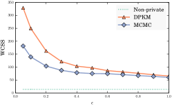
(a) S1

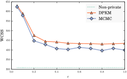
(b) Adult-num

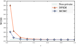
(c) Tiger

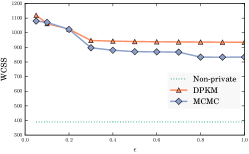
(d) Image

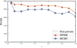
(e) Gowalla

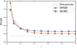
(f) Lifesci

Figure 1: WCSS by varying $\epsilon$

Figure 1 shows the performance of our post-processing algorithm for different values of $\epsilon$. The value of $\epsilon$ ranges from $0.05$ to $1.0$. The proposed algorithm improves the accuracy of the final clusterings on all datasets, except on the Lifesci dataset. On S1 and Tiger datasets, huge improvements in WCSS were observed when $\epsilon=0.05$.

References

• Blum etย al. (2005) Blum, Avrim, Dwork, Cynthia, McSherry, Frank, and Nissim, Kobbi. Practical privacy: The sulq framework. In PODS, 2005.
• Dwork & Roth (2014) Dwork, Cynthia and Roth, Aaron. The algorithmic foundations of differential privacy. Foundations and Trendsยฎ in Theoretical Computer Science, 9(3โ€“4), 2014.
• Hay etย al. (2010) Hay, Michael, Rastogi, Vibhor, Miklau, Gerome, and Suciu, Dan. Boosting the accuracy of differentially private histograms through consistency. Proc. VLDB Endow., 3(1-2):1021โ€“1032, September 2010. ISSN 2150-8097.
• Lee etย al. (2015) Lee, Jaewoo, Wang, Yue, and Kifer, Daniel. Maximum likelihood postprocessing for differential privacy under consistency constraints. In KDD, 2015.
• Lin & Kifer (2013) Lin, Bing-Rong and Kifer, Daniel. Information preservation in statistical privacy and bayesian estimation of unattributed histograms. In SIGMOD, 2013.
• McSherry (2009) McSherry, Frankย D. Privacy integrated queries: An extensible platform for privacy-preserving data analysis. In SIGMOD, 2009.
• Mohan etย al. (2012) Mohan, Prashanth, Thakurta, Abhradeep, Shi, Elaine, Song, Dawn, and Culler, David. Gupt: Privacy preserving data analysis made easy. In SIGMOD, 2012.
• Nissim etย al. (2007) Nissim, Kobbi, Raskhodnikova, Sofya, and Smith, Adam. Smooth sensitivity and sampling in private data analysis. In STOC, 2007.
• Su etย al. (2015) Su, D., Cao, J., Li, N., Bertino, E., and Jin, H. Differentially Private $k$-Means Clustering. ArXiv e-prints, April 2015.
• Zhang etย al. (2013) Zhang, Jun, Xiao, Xiaokui, Yang, Yin, Zhang, Zhenjie, and Winslett, Marianne. Privgene: Differentially private model fitting using genetic algorithms. In SIGMOD, 2013.