Thermal States and Wave Packets

Abstract

The classical and quantum representations of thermal equilibrium are strikingly different, even for free, non-interacting particles. While the first involves particles with well-defined positions and momenta, the second usually involves energy eigenstates that are delocalized over a confining volume. In this paper, we derive convex decompositions of the density operator for non-interacting, non-relativistic particles in thermal equilibrium that allow for a connection between these two descriptions. Associated with each element of the decomposition of the $N$-particle thermal state is an $N$-body wave function, described as a set of wave packets; the distribution of the average positions and momenta of the wave packets can be linked to the classical description of thermal equilibrium, while the different amplitudes in the wave function capture the statistics relevant for fermions or bosons.

Thermal states are ubiquitous in physics. In both classical and quantum statistical mechanics they play a central role in many calculations, either as an assumption of the initial state of a system of interest before a perturbation is applied, or as a description of the state of a reservoir interacting with a system of interest. In the simple textbook problem of the equilibrium state of non-interacting, non-relativistic particles confined to a box and at a given temperature, the classical results for thermodynamic quantities, such as the free energy, are easily recovered as the appropriate limits of the quantum results. But even under circumstances where a classical description should suffice, the classical and quantum descriptions of equilibrium are strikingly different. In classical statistical mechanics a distribution function is introduced, assigning well-defined momenta and positions to particles with appropriate probabilities. In quantum statistical mechanics, the usual representation of the thermal density operator is in terms of the energy eigenstates, states that are extended throughout the confining volume, with the position uncertainty in each single-particle state thus given by the size of the box itself. This is unchanging even as the temperature is increased, and the classical limit should be recovered.

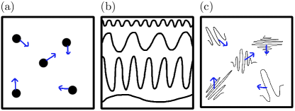
Figure 1: Illustration of various possible representations of thermal equilibrium for free, non-interacting $N$-particles. The classical picture (a) is strikingly different from the quantum picture (b). In the former, each particle has a well-defined position and momentum (blue arrows), while the latter is in terms of eigenstates that spread over the full confining volume. The sketch in (b) depicts a sample of eigenfunctions $\phi_{n}(\mathbf{r})$ (Eq. 4) describing the one-particle thermal state (Eq. 5). In the main text, we derive alternative decompositions involving wave packets with average positions and momenta. The sketch in (c) depicts the $N$-body wave function, involving a set of wave packets (Eqs. 12 and 21), and corresponding to a term in this alternative decomposition. The distribution of the average positions and momenta of the wave packets can be linked to the classical description of thermal equilibrium, such that (c) provides a connection between (a) and (b).

Since the early days of quantum mechanics, significant theoretical attention has been put into representing quantum mechanics using the language of classical physics (see, e.g., Schleich Schleich (2011)). Among the first developments is the formalism developed by Moyal Moyal (1949), which closely relates quantum operators and classical functions of phase space variables first suggested by Weyl Weyl (1927). This is based on the observation that the dynamical evolution of the Wigner function, given by the Liouville equation, takes a form identical to the evolution of the density matrix in the classical limit generalizing the Poisson brackets to Moyal brackets. Alternative approaches include phase space methods connected either to the corpuscular classical limit—coordinate-momentum phase space (see e.g. Hillery Hillery et al. (1984) et al. for a review)—or to the wave classical limit. These rely on the coherent state representation of bosonic systems Gardiner and Zoller (2004); Walls and Milburn (2007), which have largely influenced the concepts in quantum optics Fano (1983) and have since found many applications. It was recently shown how the coordinate-momentum and the bosonic coherent state phase-space representations can be identically mapped to each other under the change of variables Polkovnikov (2010).

The phase space representation of quantum systems is not unique. Focusing on the description of an ideal gas, we here present an alternative representation in coordinate-momentum space that involves a many-body wave function with classical-like variables, and connects the quantum and classical representations of thermal equilibrium. Such a microscopic description of the Gibbs ensemble can assist in deriving thermodynamical quantities from microscopic theory, a question that has attracted attention over the years Balian (2007) and has remained a subject of debate since the foundations were laid (see e.g. D’Alessio et al. (2016) for a review). In a broader context, and despite known analogies between quantum and classical systems Strocchi (1966); Frank and von Brentano (1994); Alzar et al. (2002); Novotny (2010); Elze (2012); Briggs and Eisfeld (2012), no general approach has been successful in establishing a classical representation for statistical mixtures.

Thermal states are statistical mixtures, and so are usually represented using the density matrix formalism Fano (1957). Yet a density matrix generally allows many representations, or ‘convex decompositions’. . In this paper we construct, for a canonical ensemble describing non-interacting, non-relativistic particles, convex decompositions of the density operator that involve sets of wave packets, each wave packet with a localized coordinate representation and an expectation value of momentum. The first decomposition we give is in terms of static wave-packets. While this is straightforward for the one-particle subspace, we generalize this decomposition to a many-body formalism using field theory. More importantly, we derive an alternative basis that involves dynamic wave-packets and provide a full class of new convex decompositions. We can then see explicitly how the classical particle picture arises as a limit of the quantum wavepackets; see Fig. (1) for a sketched illustration. The classical limit for the partition function that follows has been studied previously (see, e.g., Huang Huang (1987)). Our approach goes beyond these treatments in that we consider the quantum state itself rather than its thermodynamic properties.

Given the importance of thermal states in physics, the study of different convex decompositions of the canonical ensemble is an interesting problem in itself. There are also practical applications. Earlier Hornberger and Sipe (2003), a wave packet decomposition of the Maxwell-Boltzmann limit helped in the study of decoherence of a heavy quantum Brownian particle interacting with a background gas. By representing the ideal gas as an ensemble of quantum particles, its effect on the coherence of the Brownian particle could be obtained from calculating a single scattering event, and averaging over all events to account for the thermal mixture. This theory provided the framework for understanding quantum decoherence experiments with large particles such as $C_{70}$ fullerene Hornberger et al. (2004); Hackermüller et al. (2004). But in Hornberger and Sipe (2003); Hornberger et al. (2004); Hackermüller et al. (2004) the gas particles were explicitly treated as distinguishable; here we employ field theory to treat the equilibrium of non-interacting fermions or bosons, and construct convex decompositions of the density operator even at low temperatures where indistinguishability issues arise. Of course, in the classical limit the Maxwell-Boltzmann results arise naturally as a special case of the calculation we present in this paper, but the extensions to fermions and bosons presented here should allow for more general studies of decoherence.

The outline of the paper is as follows. In Sec. I we present a field theory form of the density operator describing the canonical ensemble for free particles, and indicate the standard quantum-mechanical representation. In Sec. II we present the general method used here to derive an alternative convex decomposition, which is applied for a one-particle ensemble in Sec. III and generalized for any number of particles in Sec. IV. We illustrate how our new decomposition brings insights in the calculation of thermodynamics quantities, specifically the partition function and correlation functions, in Sec. V. Conclusions and connections to previous work, and a generalization to the grand canonical ensemble, are presented in the final section.

I The canonical ensemble

We consider non-interacting, non-relativistic bosons or fermions of mass $m$ confined by a square potential energy $v(\mathbf{r})$ that vanishes everywhere expect on the edges, taken at a large distance $L$ away from the origin, thus defining a “nominal confining box.” Neglecting spin degrees of freedom, which could be easily included, the Hamiltonian is given by

$$H=\int\psi^{\dagger}(\mathbf{r})\left(-\frac{\hbar^{2}}{2m}\nabla^{2}+v(\mathbf{r})\right)\psi(\mathbf{r})d\mathbf{r},$$ (1)

where the operators $\psi^{\dagger}(\mathbf{r})$ and $\psi(\mathbf{r})$ respectively create and annihilate a particle at position $\mathbf{r}$ and fulfill the commutation relations $\left[\psi(\mathbf{r}),\psi^{\dagger}(\mathbf{r}^{\prime})\right]_{\pm}=\delta(\mathbf{r}-\mathbf{r}^{\prime})$ and $\left[\psi(\mathbf{r}),\psi(\mathbf{r}^{\prime})\right]_{\pm}=0$; here and below the upper of the two signs always refers to fermions and the lower to bosons, and $[A,B]_{\pm}\equiv AB\pm BA$. Most discussions of thermal equilibrium of such systems using field theory employ a grand canonical ensemble, where the number of particles can fluctuate. We turn to this later in the paper, but mainly consider the canonical ensemble, where the number of particles is fixed. The relevant subspace $\mathcal{H}^{(N)}$ of $N$ particles is identified by the identity operator acting over that subspace,

$$\begin{split}\mathbbm{1}^{(N)}\equiv{}&\frac{1}{N!}\int d\mathbf{r}_{1}\dots d\mathbf{r}_{N}\\ \times&\psi^{\dagger}(\mathbf{r}_{1})\dots\psi^{\dagger}(\mathbf{r}_{N})|\mathrm{vac}\rangle\langle\mathrm{vac}|\psi(\mathbf{r}_{N})\dots\psi(\mathbf{r}_{1}),\end{split}$$ (2)

where $|\mathrm{vac}\rangle$ indicates the vacuum state with no particles; this expression is valid for either fermions or bosons. The density operator for a canonical ensemble involving $N$ particles can then be constructed by replacing the Hamiltonian (1) in the usual Boltzmann factor $\exp(-\beta H)$ by its projection onto $\mathcal{H}^{(N)}$, i.e. $H\rightarrow\mathbbm{1}^{(N)}H\mathbbm{1}^{(N)}$. Since the full Hamiltonian (1) does not change the number of particles, it commutes with $\mathbbm{1}^{(N)}$, and we can write the density operator for a canonical ensemble of $N$ particles at temperature $T$ in a particular form that will prove convenient,

$$\rho{{}_{\mathrm{th}}^{(N)}}=\frac{1}{Z^{(N)}}\>e^{-\beta H/2}\mathbbm{1}^{(N)}\>e^{-\beta H/2},$$ (3)

where $Z^{(N)}$ is the partition function for $N$ particles, $\beta=1/k_{B}T$, and $k_{B}$ is Boltzmann’s constant; the expression $Z^{(N)}=\mathrm{Tr}[\mathbbm{1}^{(N)}e^{-\beta H}]$ follows from the normalization condition $\mathrm{Tr}[\rho_{\rm th}^{(N)}]=1.$

A starting point for our work below will be the density operator for a single particle, $\rho_{\rm th}^{(1)}$. The usual convex decomposition is obtained from the equations above by expanding the field operator in terms of the energy eigenstates, $\psi(\mathbf{r})=\sum_{n}a_{n}\phi_{n}(\mathbf{r})$, where $[a_{n},a_{n^{\prime}}^{\dagger}]_{\pm}=\delta_{nn^{\prime}}$ and

$$\left(-\frac{\hbar^{2}}{2m}\nabla^{2}+v(\mathbf{r})\right)\phi_{n}(\mathbf{r})=E_{n}\phi_{n}(\mathbf{r}).$$ (4)

Using the eigenstates in (2) for $\mathbbm{1}^{(1)}$ and putting that result in (3), we find the usual convex decomposition,

$$\rho{{}_{\mathrm{th}}^{(1)}}=\sum_{n=0}^{\infty}|n\rangle p_{n}\langle n|$$ (5)

with $\left|n\right\rangle=a_{n}^{\dagger}|\mathrm{vac}\rangle$, $p_{n}=\exp(-\beta E_{n})/Z^{(1)}$, and $Z^{(1)}=\sum_{n}\exp(-\beta E_{n})$. Instead of actually constructing the wave functions $\phi_{n}(\mathbf{r})$ and their energies $E_{n}$ for a particular potential $v(\mathbf{r})$, often one assumes that the square potential $v(\mathbf{r})$ vanishes within a very large cubical box of volume $V=L^{3}$ and is essentially infinite outside it, confining the particle to the box; further, instead of using the standing wave solutions of the resulting Hamiltonian, in place of $\phi_{n}(\mathbf{r})$ one simply takes plane waves, $L^{-3/2}\exp(i\mathbf{k\cdot\mathbf{r})}$, satisfying periodic boundary conditions by requiring $k_{i}=2\pi n_{i}/L$ for each Cartesian component of $\mathbf{k}$, where the $n_{i}$ are integers Combescot and Shiau (2016). Then $n=\left\{n_{x},n_{y},n_{z}\right\}$, $E_{n}=\hbar^{2}(k_{x}^{2}+k_{y}^{2}+k_{z}^{2})/(2m)$, and in the limit $V\rightarrow\infty$ the standard result is $Z^{(1)}\rightarrow V/\lambda^{3}$, where $\lambda\equiv\sqrt{2\pi\hbar^{2}\beta/m}$ is the thermal de Broglie wavelength. This is a good approximation for $\lambda^{3}/V\ll 1$; we present a new argument for this below, and show how corrections to this limit could be included if desired. But note that whether the $\phi_{n}(\mathbf{r})$ satisfying (4) are adopted, or plane waves used in their stead, the wave functions associated with the states appearing in the convex decomposition (5) are delocalized throughout the entire box confining the particles—as sketched in Fig. 1(b).

II Wave packets

In contrast, we now introduce a strategy for rewriting $\rho_{\rm th}^{(N)}$ that for $N=1$ will lead to a convex decomposition of $\rho_{\rm th}^{(1)}$ in terms of wave packets, rather than completely delocalized wave functions as in (5), and for arbitrary $N$ will lead to a convex decomposition of $\rho_{\rm th}^{(N)}$ in terms of sets of wave packets. The strategy is based on finding an operator $\mathcal{O^{\dagger}}(\mathbf{r})$ such that

$$e^{-\beta H/2}\psi^{\dagger}(\mathbf{r})=\mathcal{O^{\dagger}}(\mathbf{r})e^{-\beta H/2}.$$ (6)

Once this is identified, we can “pull through” the factors $e^{-\beta H/2}$ appearing in the expression (3) for the density operator of the canonical ensemble until they act on the vacuum, which then simply yields the vacuum state itself. The result is

$$\begin{split}\rho_{\rm th}^{(N)}={}&\frac{1}{N!}\frac{1}{Z^{(N)}}\int d\mathbf{r}_{1}d\mathbf{r}_{2}\cdots d\mathbf{r}_{N}\\ &\times\mathcal{O^{\dagger}}(\mathbf{r}_{1})\mathcal{O^{\dagger}}(\mathbf{r}_{2})\mathcal{\cdots O^{\dagger}}(\mathbf{r}_{N})|\mathrm{vac}\rangle\\ &\times\langle\mathrm{vac}|\mathcal{O}(\mathbf{r}_{N})\cdots\mathcal{O}(\mathbf{r}_{2})\mathcal{O}(\mathbf{r}_{1}),\end{split}$$ (7)

a convex decomposition involving states that we shall see are $N$-particle wave packets identified by $\mathcal{O^{\dagger}}(\mathbf{r}_{1})\mathcal{O^{\dagger}}(\mathbf{r}_{2})\mathcal{\cdots O^{\dagger}}(\mathbf{r}_{N})|\mathrm{vac}\rangle$.

To determine $\mathcal{O^{\dagger}}(\mathbf{r})$ we introduce $\Psi^{\dagger}(\mathbf{r},\nu)\equiv e^{-\nu H/2}\psi^{\dagger}(\mathbf{r})e^{\nu H/2}$; then $\Psi^{\dagger}(\mathbf{r},0)=\psi^{\dagger}(\mathbf{r})$ and $\Psi^{\dagger}(\mathbf{r},\beta)=\mathcal{O^{\dagger}}(\mathbf{r})$. We easily find

$$\begin{split}\frac{\partial\Psi^{\dagger}(\mathbf{r},\nu)}{\partial\nu}&=\frac{1}{2}e^{-\nu H/2}\left[\psi^{\dagger}(\mathbf{r}),H\right]_{-}e^{\nu H/2}\\ &=\frac{\hbar^{2}}{4m}\nabla^{2}\Psi^{\dagger}(\mathbf{r},\nu)-\frac{1}{2}v(\mathbf{r})\Psi^{\dagger}(\mathbf{r},\nu),\end{split}$$ (8)

where although only the commutator arises from the differentiation, the result holds whether we consider bosons or fermions. This is a typical diffusion equation, and with the initial condition at $\nu=0$, $\Psi^{\dagger}(\mathbf{r},0)=\psi^{\dagger}(\mathbf{r})$, there are two special cases of interest: (a) if $v(\mathbf{r})$ is neglected we find the solution

$$\Psi^{\dagger}(\mathbf{r},\beta)\underset{\underset{\rm everywhere}{v(\mathbf{r})\rightarrow 0}}{\longrightarrow}\int G(\mathbf{r}-\mathbf{r^{\prime}};\lambda)\psi^{\dagger}(\mathbf{r^{\prime}})d\mathbf{r^{\prime}},$$ (9)

with

$$G(\mathbf{r}-\mathbf{r^{\prime}};\lambda)=\frac{2\sqrt{2}}{\lambda^{3}}e^{-2\pi\frac{\left|\mathbf{r}-\mathbf{r^{\prime}}\right|^{2}}{\lambda^{2}}},$$ (10)

where again $\lambda$ is the thermal de Broglie wavelength associated with $\beta$, and $G(\mathbf{r}-\mathbf{r^{\prime}};0)=\delta(\mathbf{r}-\mathbf{r^{\prime}})$; (b) if $v(\mathbf{r})$ is large and positive we have $\Psi^{\dagger}(\mathbf{r},\beta)\rightarrow 0$ as $v(\mathbf{r})\rightarrow\infty$. Recalling from (7) that $\mathcal{O^{\dagger}}(\mathbf{r})=\Psi^{\dagger}(\mathbf{r},\beta)$, we see from (b) that if any of the $\mathbf{r}_{i}$ lie far outside the nominal confining box, where $v(\mathbf{r})$ is large and positive, the contribution from $\mathcal{O^{\dagger}}(\mathbf{r}_{i})$ can be neglected. And since from (10) we see that $G(\mathbf{r}-\mathbf{r^{\prime}};\lambda)$ is non-negligible for $\left|\mathbf{r}-\mathbf{r^{\prime}}\right|$ less than or on the order of $\lambda$, we can surmise from (9) that the effect of $\mathcal{O^{\dagger}}(\mathbf{r}_{i})=\Psi^{\dagger}(\mathbf{r}_{i},\beta)$ can be described by (9) as long as $\mathbf{r}_{i}$ is within a few $\lambda$ of any edge of the nominal box and inside it. Combining these two results, if the volume $V$ of the nominal box satisfies $V\gg\lambda^{3}$, we make a negligible error restricting the integrals in (7) to the volume of the nominal confining box, and for all such points $\mathbf{r}$ within that volume, we use

$$\mathcal{O^{\dagger}}(\mathbf{r})=\int G(\mathbf{r}-\mathbf{r^{\prime}};\lambda)\psi^{\dagger}(\mathbf{r^{\prime}})d\mathbf{r^{\prime}}.\\$$ (11)

Corrections will be important as the confining volume shrinks to a size on the order of the thermal de Broglie wavelength, and indeed the approach we are developing here would be an interesting way to explore such “finite size” effects. One would simply use the more correct (7), and instead of using (10) for the Green function use the exact solution of (8). But we defer such explorations to later communications, and here restrict ourselves to a large volume and use (11) in (7) with the volume restricted to $V$.

It is convenient to introduce the normalized function $\phi_{\mathbf{r},\lambda}(\mathbf{r^{\prime})}\equiv\lambda^{3/2}G(\mathbf{r}-\mathbf{r^{\prime}};\lambda),$

$$\phi_{\mathbf{r},{\lambda}}(\mathbf{r}^{\prime})=\frac{2\sqrt{2}}{\lambda^{3/2}}e^{-2\pi\frac{|\mathbf{r}^{\prime}-\mathbf{r}|^{2}}{\lambda^{2}}},$$ (12)

with $\int\left|\phi_{\mathbf{r},\lambda}(\mathbf{r}^{\prime})\right|^{2}d\mathbf{r^{\prime}}=1$. Then, considering a large volume, we can write (6) as

$$e^{-\beta H/2}\psi^{\dagger}(\mathbf{r})=\frac{1}{\lambda^{3/2}}\left(\int\phi_{\mathbf{r},{\lambda}}(\mathbf{r}^{\prime})\psi^{\dagger}(\mathbf{r}^{\prime})d\mathbf{r}^{\prime}\right)e^{-\beta H/2},$$ (13)

for any $\mathbf{r}$ within the volume $V$. Letting (13) act on any state $\left|\xi\right\rangle$, multiplying by the adjoint and integrating over all $\mathbf{r}$ within the volume $V$, we have

$$\int_{V}d\mathbf{r}\left(e^{-\frac{\beta}{2}H}\psi^{\dagger}(\mathbf{r})|\xi\rangle\langle\xi|\psi(\mathbf{r})e^{-\frac{\beta}{2}H}\right)=\frac{V}{\lambda^{3}}\int_{V}\frac{d\mathbf{r}}{V}\left(\int d\mathbf{r}^{\prime}\>\phi_{\mathbf{r},\lambda}(\mathbf{r}^{\prime})\psi^{\dagger}(\mathbf{r}^{\prime})\right)e^{-\frac{\beta}{2}H}|\xi\rangle\langle\xi|e^{-\frac{\beta}{2}H}\left(\int d\mathbf{r}^{\prime\prime}\>\phi^{*}_{\mathbf{r},\lambda}(\mathbf{r}^{\prime\prime})\psi(\mathbf{r}^{\prime\prime})\right),$$ (14)

which is the central result of this section.

III A single particle

We now return to the example of a single particle, and use (14) to write the expression for $\rho_{\rm th}^{(1)}$ that follows from (7) as

$$\rho_{\rm th}^{(1)}=\frac{1}{Z^{(1)}}\frac{V}{\lambda^{3}}\int_{V}\frac{d\mathbf{r}}{V}\left|\Phi_{\mathbf{r},\lambda}\right\rangle\left\langle\Phi_{\mathbf{r},\lambda}\right|,$$ (15)

where we have defined the single particle state

$$|\Phi_{\mathbf{r},\lambda}\rangle\equiv\int d\mathbf{r}^{\prime}\phi_{\mathbf{r},\lambda}(\mathbf{r}^{\prime})\psi^{\dagger}(\mathbf{r}^{\prime})|\mathrm{vac}\rangle.$$ (16)

Since the single particle states $\left|\Phi_{\mathbf{r},\lambda}\right\rangle$ are normalized, $\left\langle\Phi_{\mathbf{r},\lambda}|\Phi_{\mathbf{r},\lambda}\right\rangle=1$, the condition $\mathrm{Tr}[\rho_{\rm th}^{(1)}]=1$ implies that

$$\rho_{\rm th}^{(1)}=\int_{V}\frac{d\mathbf{r}}{V}\left|\Phi_{\mathbf{r},\lambda}\right\rangle\left\langle\Phi_{\mathbf{r},\lambda}\right|.$$ (17)

Comparison with (15) leads immediately to the result $Z^{(1)}=V/\lambda^{3}$, as would be expected.

Each single-particle state $\left|\Phi_{\mathbf{r},\lambda}\right\rangle$ has a coordinate representation $\langle\mathrm{vac}|\psi(\mathbf{r^{\prime}})\left|\Phi_{\mathbf{r},\lambda}\right\rangle=\phi_{\mathbf{r},\lambda}(\mathbf{r}^{\prime})$, which is a minimum uncertainty wave packet centered at $\mathbf{r}$ and extending about a distance $\lambda$ from $\mathbf{r}$ in all directions. In particular, for each of these states $\Delta x=\Delta y=\Delta z=\lambda/\sqrt{8\pi}$, and $\Delta p_{x}=\Delta p_{y}=\Delta p_{z}=\sqrt{2\pi}\hbar/\lambda$. Note that the expectation value of the momentum in each wave packet $\phi_{\mathbf{r},\lambda}(\mathbf{r^{\prime})}$ vanishes, but

$$\frac{\left(\Delta p_{x}\right)^{2}+\left(\Delta p_{y}\right)^{2}+\left(\Delta p_{z}\right)^{2}}{2m}=\frac{3}{2}k_{B}T.$$ (18)

That is, in (17) we have the density operator written as a mixture of localized wave packets, distributed in their mean positions over the box containing the particle, but the expectation value of the momentum of each wave packet vanishes, and the thermal energy is completely contained in the width of the wave packet. A convex decomposition more in line with the classical picture of thermal equilibrium would involve localized wave packets with expectation values of momentum (Fig. 1c), but averaged over all possible momenta with an appropriate probability distribution such that the average momentum of course vanishes.

Following a strategy introduced earlier Hornberger and Sipe (2003), we can move to such a convex decomposition by noting that when (16) is substituted into (17), terms such as $\phi_{\mathbf{r},\lambda}(\mathbf{r^{\prime}})\phi_{\mathbf{r},\lambda}^{*}(\mathbf{r}^{\prime\prime})$ appear, which are then to be integrated over $\mathbf{r}$. That integral extends over the volume $V$ of the box, but for the $\mathbf{r}^{\prime}$ and $\mathbf{r}^{\prime\prime}$ of importance, it can be extended over infinity without serious error, within our usual assumption of $V/\lambda^{3}\gg 1$. So for the $\mathbf{r}^{\prime}$ and $\mathbf{r}^{\prime\prime}$ of importance we can write

$$\begin{split}\int_{V}d\mathbf{r}&\phi_{\mathbf{r},\lambda}(\mathbf{r^{\prime}})\phi_{\mathbf{r},\lambda}^{*}(\mathbf{r}^{\prime\prime})\approx\int d\mathbf{r}\phi_{\mathbf{r},\lambda}(\mathbf{r^{\prime}})\phi_{\mathbf{r},\lambda}^{*}(\mathbf{r}^{\prime\prime})\\ &=e^{-\pi\frac{\left|\mathbf{r^{\prime}}-\mathbf{r^{\prime}}^{\prime}\right|^{2}}{\lambda^{2}}}\\ &=\int d\mathbf{r}\int d\mathbf{p}f_{\lambda_{m}}(\mathbf{p})\phi_{\mathbf{r}\mathbf{p},\lambda_{s}}(\mathbf{r^{\prime}})\phi_{\mathbf{r}\mathbf{p},\lambda_{s}}^{*}(\mathbf{r}^{\prime\prime})\\ &\approx\int_{V}d\mathbf{r}\int d\mathbf{p}f_{\lambda_{m}}(\mathbf{p})\phi_{\mathbf{r}\mathbf{p},\lambda_{s}}(\mathbf{r^{\prime}})\phi_{\mathbf{r}\mathbf{p},\lambda_{s}}^{*}(\mathbf{r}^{\prime\prime}).\end{split}$$ (19)

In the second strict equality we have introduced a normalized momentum distribution function,

$$\begin{split}f_{\lambda_{m}}(\mathbf{p})=\left(\frac{\lambda_{m}}{2\pi\hbar}\right)^{3}e^{-\lambda_{m}^{2}\mathbf{p}^{2}/(4\pi\hbar^{2})},\end{split}$$ (20)

with $\int f_{\lambda_{m}}(\mathbf{p})d\mathbf{p}=1$, and a set of normalized wave functions,

$$\begin{split}\phi_{\mathbf{r}\mathbf{p},\lambda_{s}}(\mathbf{r}^{\prime})&=\frac{2\sqrt{2}}{\lambda_{s}^{3/2}}e^{i\mathbf{p}\cdot(\mathbf{r}^{\prime}-\mathbf{r})/\hbar}e^{-2\pi|\mathbf{r}^{\prime}-\mathbf{r}|^{2}/\lambda_{s}^{2}},\end{split}$$ (21)

with $\int\left|\phi_{\mathbf{r}\mathbf{p},\lambda_{s}}(\mathbf{r}^{\prime})\right|^{2}d\mathbf{r^{\prime}}=1$. That strict equality holds as long as we choose $\lambda_{s}$ and $\lambda_{m}$ such that $\lambda^{-2}=\lambda_{s}^{-2}+\lambda_{m}^{-2}$. Associating $\lambda_{s}$ and $\lambda_{m}$ with temperatures $T_{s}$ and $T_{m}$ respectively, through the relation of a thermal de Broglie wavelength to temperature, this condition requires $T=T_{s}+T_{m}$. We comment on the physical significance of $\lambda_{s}$ and $\lambda_{m}$ below, but we note that for $\mathbf{r}^{\prime}$ and $\mathbf{r}^{\prime\prime}$ of importance the last approximate result of (19) follows if $\lambda_{s}$ is not too small, and that last result can then be applied for all $\mathbf{r}^{\prime}$ and $\mathbf{r}^{\prime\prime}$ within our usual assumption that $V\gg\lambda^{3}$. Finally, inserting (16) in (17) and using (19), we find an alternate convex decomposition of $\rho_{\rm th}^{(1)}$,

$$\rho_{\rm th}^{(1)}=\int_{V}\frac{d\mathbf{r}}{V}\int d\mathbf{p}f_{\lambda_{m}}(\mathbf{p})\left|\Phi_{\mathbf{r}\mathbf{p},\lambda_{s}}\right\rangle\left\langle\Phi_{\mathbf{r}\mathbf{p},\lambda_{s}}\right|$$ (22)

in terms of single particle states

$$|\Phi_{\mathbf{r}\mathbf{p},\lambda_{s}}\rangle\equiv\int d\mathbf{r}^{\prime}\phi_{\mathbf{r}\mathbf{p},\lambda_{s}}(\mathbf{r}^{\prime})\psi^{\dagger}(\mathbf{r}^{\prime})|\mathrm{vac}\rangle.$$ (23)

These are again minimum uncertainty states, but each has an expectation value $\mathbf{p}$ of momentum, and $\Delta x=\Delta y=\Delta z=\lambda_{s}/\sqrt{8\pi}$, and $\Delta p_{x}=\Delta p_{y}=\Delta p_{z}=\sqrt{2\pi}\hbar/\lambda_{s}$. That is, these wave packets are broader than those introduced in (17). So instead of (18), for these wave packets we have

$$\begin{split}\frac{\left(\Delta p_{x}\right)^{2}+\left(\Delta p_{y}\right)^{2}+\left(\Delta p_{z}\right)^{2}}{2m}&=\frac{3}{2}k_{B}T_{s},\\ \int\frac{p_{x}^{2}+p_{y}^{2}+p_{z}^{2}}{2m}f_{\lambda_{m}}(\mathbf{p})d\mathbf{p}&=\frac{3}{2}k_{B}T_{m}.\\ \end{split}$$ (24)

That is, part of the thermal energy resides in the motion of the wave packets, and part of it resides in their width.

For the purpose of illustration, consider argon atoms at room temperature ($\lambda=0.16$Å) Waber and Cromer (1965). In the convex decomposition (17) involving the most localized wave packets, the wave packet FWHM is $0.07\textrm{\AA}$. Even in a convex decomposition (22) that would involve wave packets with only $1\%$ of the kinetic energy residing in the width of the wave packets ($T_{s}=3K),$ and the remaining $99\%$ in the mean velocities of the wave packets, the wave packet FWHM would be only $0.75\textrm{\AA}$, which would be on the order of the diameter of the outermost orbital of the argon electrons ($1.3\textrm{\AA}).$ Thus the construction of a convex decomposition of the form (22) involving classical-like motion of wave packets is certainly possible in the classical regime, as one would expect physically.

IV Generalization to $N$ particles

The generalization to a canonical ensemble of $N$ particles follows immediately, applying (13) to (7) $N$ times, “pulling through” $\exp(-\beta H/2)$ until it acts on the vacuum state. We find

$$\begin{split}\rho{{}_{\mathrm{th}}^{(N)}}={}&\frac{1}{N!}\frac{1}{Z^{(N)}}\left(\frac{V}{\lambda^{3}}\right)^{N}\int_{V}\frac{d\mathbf{r}_{1}\dots d\mathbf{r}_{N}}{V^{N}}\\ &\times\int d\mathbf{p}_{1}\dots d\mathbf{p}_{N}f_{\lambda_{m}}(\mathbf{p}_{1})\dots f_{\lambda_{m}}(\mathbf{p}_{N})\\ &\times|\Phi_{\mathbf{r}_{1}\mathbf{p}_{1}\dots\mathbf{r}_{N}\mathbf{p}_{N},\lambda_{s}}\rangle\langle\Phi_{\mathbf{r}_{1}\mathbf{p}_{1}\dots\mathbf{r}_{N}\mathbf{p}_{N},\lambda_{s}}|,\end{split}$$ (25)

involving $N$-particle states with localized wave packets,

$$|\Phi_{\mathbf{r}_{1}\mathbf{p}_{1}\dots\mathbf{r}_{N}\mathbf{p}_{N},\lambda_{s}}\rangle \equiv{}\left(\int d\mathbf{r}^{\prime}\>\phi_{\mathbf{r}_{1}\mathbf{p}_{1},\lambda_{s}}(\mathbf{r}^{\prime})\psi^{\dagger}(\mathbf{r}^{\prime})\right)\times\dots$$

$$\dots\times\Big{(}\int d\mathbf{r}^{\prime\prime} \>\phi_{\mathbf{r}_{N}\mathbf{p}_{N},\lambda_{s}}(\mathbf{r}^{\prime\prime})\psi^{\dagger}(\mathbf{r}^{\prime\prime})\Big{)}|\mathrm{vac}\rangle,$$ (26)

where $(\mathbf{r}_{1},\dots,\mathbf{r}_{N})$ and $(\mathbf{p}_{1},\dots,\mathbf{p}_{N})$ label the expectation values of the positions and momenta of the wave packets, respectively.

While the thermal state density matrix has unit trace, $\mathrm{Tr}[\rho{{}_{\mathrm{th}}^{(N)}}]=1$, the individual states (IV) are not normalized, and their norm encompass all features distinguishing fermionic from bosonic statistics. This becomes obvious when we use the unit trace condition to identify the partition function,

$$\begin{split}Z^{(N)}={}&\frac{1}{N!}\left(\frac{V}{\lambda^{3}}\right)^{N}\int\frac{d\mathbf{r}_{1}\dots d\mathbf{r}_{N}}{V^{N}}\\ &\times\int d\mathbf{p}_{1}\dots d\mathbf{p}_{N}f_{\lambda_{m}}(\mathbf{p}_{1})\dots f_{\lambda_{m}}(\mathbf{p}_{N})\\ &\times\left\langle{\Phi_{\mathbf{r}_{1}\mathbf{p}_{1}\dots\mathbf{r}_{N}\mathbf{p}_{N},\lambda_{s}}}|{\Phi_{\mathbf{r}_{1}\mathbf{p}_{1}\dots\mathbf{r}_{N}\mathbf{p}_{N},\lambda_{s}}}\right\rangle.\end{split}$$ (27)

The factor $(1/N!)$ is the standard Gibbs factor Huang (1987) that corrects the naive classical expression $(V/\lambda^{3})^{N}$ for the indistinguishability of the particles, and their product is the usual result in the Maxwell-Boltzmann limit. The remaining integral encapsulates the differences in the sum over states between bosonic and fermionic systems.

V Illustrations

We now present some illustrations of our results. We begin with the partition function for a system of $N=2$ particles. Of course, we recover the usual expression for the partition function

$$\begin{split}Z^{(2)}=\frac{1}{2!}\left(\frac{V}{\lambda^{3}}\right)^{2}\left(1\mp\frac{\lambda^{3}}{V}\frac{1}{2\sqrt{2}}\right),\end{split}$$ (28)

which shows the quantum correction to the classical partition function (cf. second term on the r.h.s.). This recovers the result for the first quantum corrections examined by Huang Huang (1987): the symmetry properties of the 2-particle wave function can be effectively accounted for with an attractive (repulsive) ‘statistical potential’ for bosons (fermions), which depends on the temperature and therefore cannot be regarded as a true inter-particle potential. Note that this term vanishes in the Maxwell-Boltzmann limit ($\lambda\rightarrow 0$), and thus recovers the classical result. Importantly, our approach differs from that of Huang Huang (1987) and other approaches conventionally presented in text books in that we consider the quantum state itself rather than the thermodynamics properties (derived from the partition function) to describe the ensemble.

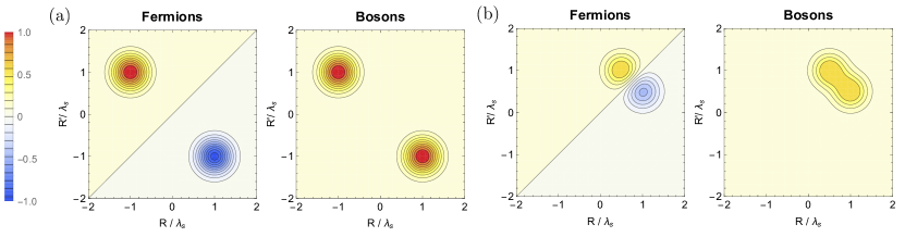
Figure 2: Coordinate representations of a 2-particle wave packet (30) for fermions and bosons with different relative centers. The average position of one wave-packet is fixed at $r_{1}/\lambda_{s}=1$. (a) When the average positions of the wave packets are separated by a few $\lambda_{s}$ ($r_{2}/\lambda_{s}=-1$) the wave packets describe distinguishable particles, and the description thereby recovers the Maxwell-Boltzmann limit. (b) When the distance between the two centres is small, e.g. (b) $r_{2}/\lambda_{s}=0.5$, the wave packets overlap, and we clearly see the anti-symmetry (symmetry) characterizing fermionic (bosonic) particles. Note that because the states (IV) are not normalized by construction the wave packets in (a) and (b) have different amplitudes. All vectors are taken to lie along a line (e.g. along the $\pm\hat{x}$ direction); all average momenta are zero here, i.e. $p_{1}=p_{2}=0$.

As mentioned below Eq. (IV), the states introduced there are not normalized, and their norm depends on the nature of the particles:

$$\left\langle\Phi_{\mathbf{r}_{1}\mathbf{r}_{2},\lambda}|\Phi_{\mathbf{r}_{1}\mathbf{r}_{2},\lambda}\right\rangle=1\mp\,e^{-\frac{2\pi}{\lambda^{2}}|\mathbf{r}_{1}-\mathbf{r}_{2}|^{2}}.$$ (29)

The norm encompasses the different permutation rules for bosons or fermions which gives rise to different quantum statistics. This can also be seen in Fig. (2), where we illustrate the coordinate representation of the 2-particle wave packet,

$$\frac{1}{\sqrt{2}}\langle\mathrm{vac}|\psi(\mathbf{R})\psi(\mathbf{R}^{\prime})|\Phi_{\mathbf{r}_{1}\mathbf{p}_{1}\mathbf{r}_{2}\mathbf{p}_{2},\lambda_{s}}\rangle=\frac{1}{\sqrt{2}}\Big{(}\phi_{\mathbf{r}_{1}\mathbf{p}_{1},\lambda_{s}}(\mathbf{R}^{\prime})\phi_{\mathbf{r}_{2}\mathbf{p}_{2},\lambda_{s}}(\mathbf{R})\mp\,\phi_{\mathbf{r}_{1}\mathbf{p}_{1},\lambda_{s}}(\mathbf{R})\phi_{\mathbf{r}_{2}\mathbf{p}_{2},\lambda_{s}}(\mathbf{R}^{\prime})\Big{)},$$ (30)

that is symmetric under exchange of coordinates for bosons, and anti-symmetric for fermions. If the density is low enough that for most $\mathbf{r}_{1}$ and $\mathbf{r}_{2}$ the wave packets appearing in the coordinate representation of the kets (and bras) in the convex decomposition (25) of $\rho{{}_{\mathrm{th}}^{(2)}}$ do not overlap, then to a good approximation the coordinate representations of the outer products of the kets and bras arising in (25) can be reorganized into terms involving simple products of two wave packets, as would be expected in the Maxwell-Boltzmann limit of distinguishable particles. This scenario generalizes to $\rho{{}_{\mathrm{th}}^{(N)}}$.

We now turn to correlations functions, which often enter in calculations involving thermal states. The $j^{\rm th}$ order correlation function for an $N$-particle thermal state is defined as

$$G^{(j)}_{\textrm{th}}(\mathbf{R}_{1}t_{1},\dots,\mathbf{R}_{j}t_{j};\mathbf{R}_{j+1}t_{j+1},\dots,\mathbf{R}_{2j}t_{2j})\equiv\mathrm{Tr}^{(N)}\Big{[}\rho{{}_{\mathrm{th}}^{(N)}}\psi^{\dagger}(\mathbf{R}_{1}t_{1})\dots\psi^{\dagger}(\mathbf{R}_{j}t_{j})\psi(\mathbf{R}_{j+1}t_{j+1})\dots\psi(\mathbf{R}_{2j}t_{2j})\Big{]},$$ (31)

where $\psi^{\dagger}(\mathbf{R}t)$ is the Heisenberg representation of the creation operator. Since our convex decomposition (22) involves localized wave packets, the correlation functions can be written as integrals over correlation functions associated with states consisting of sets of wave packets. Consider first a single-particle system. From (22), we find that the first-order correlation function can be written as

$$G^{(1)}_{\textrm{th}}(\mathbf{R}_{1}t_{1};\mathbf{R}_{2}t_{2})=\int\frac{d\mathbf{r}}{V}\int d\mathbf{p}f_{\lambda_{m}}(\mathbf{p})G^{(1)}_{\mathbf{r}\mathbf{p},\lambda_{s}}(\mathbf{R}_{1}t_{1};\mathbf{R}_{2}t_{2}),$$ (32)

where the correlation function associated with the state $\left|\Phi_{\mathbf{r}\mathbf{p},\lambda_{s}}\right\rangle$ is given by

$$G^{(1)}_{\mathbf{r}\mathbf{p},\lambda_{s}}(\mathbf{R}_{1}t_{1};\mathbf{R}_{2}t_{2})\equiv\langle\Phi_{\mathbf{r}\mathbf{p},\lambda_{s}}|\psi^{\dagger}(\mathbf{R}_{1}t_{1})\psi(\mathbf{R}_{2}t_{2})|\Phi_{\mathbf{r}\mathbf{p},\lambda_{s}}\rangle.$$ (33)

Each of these state correlation functions can be written as $G^{(1)}_{\mathbf{r}\mathbf{p},\lambda_{s}}(\mathbf{R}_{1}t_{1};\mathbf{R}_{2}t_{2})=\mathscr{F}_{\mathbf{r}\mathbf{p},\lambda_{s}}(\mathbf{R}_{1}t_{1})\mathscr{F}^{*}_{\mathbf{r}\mathbf{p},\lambda_{s}}(\mathbf{R}_{2}t_{2}),$ where we have introduced the function

$$\mathscr{F}_{\mathbf{r}\mathbf{p},\lambda_{s}}(\mathbf{R}t)\equiv{} \left(\frac{2}{\lambda(1+2ib)}\right)^{\frac{3}{2}}e^{-\frac{1}{8\pi}\left(\frac{\lambda_{s}\mathbf{p}}{\hbar}\right)^{2}}$$

$$\times e^{{-\frac{2\pi}{1+2ib}\left(\frac{\mathbf{r}-\mathbf{R}}{\lambda_{s}}-\frac{i}{4\pi}\frac{\lambda_{s}\mathbf{p}}{\hbar}\right)^{2}}},$$ (34)

with $b\equiv t/(\beta\hbar)$. Fig. 3 illustrates the first-order correlation function (33) for (a) static wave packets (zero average momentum), and (b) dynamic wave packets.

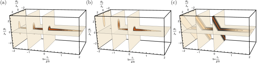
Figure 3: Absolute value of the first-order correlation function (a;b) Eq. (33) for the single-particle state (23) centred at $r=0$ with $t_{2}=0$ and an average momentum of (a) $p=0$, (b) $\lambda p/\hbar=5$; (c) Eq. (35) for a one-particle thermal state, as a function of the measurement time $t_{1}$ and space points $\mathbf{R}_{1},\mathbf{R}_{2}$. Comparing (a) with (b) shows how the wave-packet average momentum shifts the center of the correlation function in the plane $(\mathbf{R}_{1},\mathbf{R}_{2})$ as a function of time, exhibiting the motion of the wave-packet center. Averaging each of the single-state contributions of either type (a) or type (b) according to (32) recovers (c), the first-order correlation function of the complete one-particle thermal state (35), which only depends on the differences $\left|\mathbf{R}_{2}-\mathbf{R}_{1}\right|$ and $(t_{2}-t_{1})$. All vectors are taken to lie along a line.

Since the individual expectation values (33) involve a single wave packet, each of these wave packet contributions are products of functions of $(\mathbf{R}_{1},t_{1})$ and $(\mathbf{R}_{2},t_{2})$, but the integral over all these contributions (32) gives a correlation function

$$G^{(1)}_{\textrm{th}}(\mathbf{R}_{1}t_{1};\mathbf{R}_{2}t_{2})={} \frac{1}{V}\left(1+i\frac{t_{2}-t_{1}}{\beta\hbar}\right)^{-\frac{3}{2}}$$ (35)

$$\times e^{{-\frac{\pi}{1+i\frac{t_{2}-t_{1}}{\beta\hbar}}\left|\frac{\mathbf{R}_{2}-\mathbf{R}_{1}}{\lambda}\right|^{2}}}$$

that depends only on $\left|\mathbf{R}_{2}-\mathbf{R}_{1}\right|$ and $(t_{2}-t_{1})$, as illustrated in Fig. 3c.

We now turn to a system with $N=2$ particles. If we consider the first order correlation function we will find contributions from each state in (25), with each contribution arising from a first order correlation function of a state with two wave packets. Here the nature of the particles will appear explicitly. For example, if we consider a state involving two wave packets with no average momentum, $p_{1}=p_{2}=0$, we find

$$\begin{split}G^{(1)}_{\mathbf{r}_{1}0\mathbf{r}_{2}0,\lambda_{s}}(\mathbf{R}_{1}t_{1};\mathbf{R}_{2}t_{2})\equiv{}&\langle\Phi_{\mathbf{r}_{1}0\mathbf{r}_{2}0,\lambda_{s}}|\Psi^{\dagger}(\mathbf{R}_{1}t_{1})\ \Psi(\mathbf{R}_{2}t_{2})|\Phi_{\mathbf{r}_{1}0\mathbf{r}_{2}0,\lambda_{s}}\rangle\\ ={}&G^{(1)}_{\mathbf{r}_{1}0,\lambda_{s}}(\mathbf{R}_{1}t_{1};\mathbf{R}_{2}t_{2})+G^{(1)}_{\mathbf{r}_{2}0,\lambda_{s}}(\mathbf{R}_{1}t_{1};\mathbf{R}_{2}t_{2})\\ &\mp e^{-\pi\frac{|\mathbf{r}_{1}-\mathbf{r}_{2}|^{2}}{\lambda_{s}^{2}}}\Big{(}\mathscr{F}_{\mathbf{r}_{1}0,\lambda_{s}}(\mathbf{R}_{1}t_{1})\mathscr{F}_{\mathbf{r}_{2}0,\lambda_{s}}^{*}(\mathbf{R}_{2}t_{2})+\mathscr{F}_{\mathbf{r}_{2}0,\lambda_{s}}(\mathbf{R}_{1}t_{1})\mathscr{F}^{*}_{\mathbf{r}_{1}0,\lambda_{s}}(\mathbf{R}_{2}t_{2})\Big{)},\end{split}$$ (36)

where note that the contribution involves a single-particle term from each wave packet, plus quantum corrections that appear for overlapping wave-functions (see Fig. 4). In the Maxwell-Boltzmann limit the contribution from these correction terms will become negligible, as indeed they will be for an $N$ particle system, and the first order correlation function then reduces to the contributions from the individual wave packets,

$$G^{(1)}_{\mathbf{r}_{1}\dots\mathbf{r}_{N}0\dots 0,\lambda}(\mathbf{R}_{1}t_{1};\mathbf{R}_{2}t_{2})\longrightarrow\sum_{n=1}^{N}G^{(1)}_{\mathbf{r}_{n}0,\lambda}(\mathbf{R}_{1}t_{1};\mathbf{R}_{2}t_{2}).$$ (37)

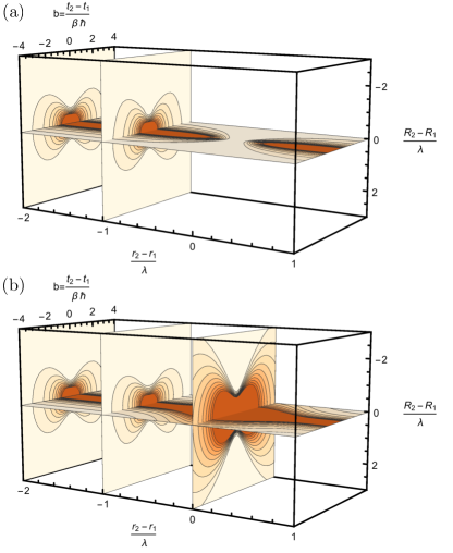
Figure 4: First-order correlation function (36) for the 2-particle states for (a) fermions and (b) bosons. We clearly see the consequence of Pauli exclusion principle and the anti-bunching character of fermions, leading to a zero correlation function for overlapping wave packets (${|\mathbf{r}_{2}-\mathbf{r}_{1}|}/{\lambda}=0$). In contrast, the bosons (b) present an enhanced correlation function due to their bunching character. For non-overlapping wave functions (${|\mathbf{r}_{2}-\mathbf{r}_{1}|}/{\lambda}\gg 1$), both fermionic and bosonic systems exhibit the same properties and we recover the Maxwell-Boltzmann limit, i.e. a profile similar to Fig. (3a) for individual particles. All vectors are taken to lie along a line (e.g. along the $\pm\hat{x}$ direction).

VI Outlook and Conclusions

We have shown that an $N$-particle thermal state can be represented by a mixture of $N$-particle localized wave-packets, and have given expressions for such decompositions. From these decompositions, one can see explicitly how the classical particle picture arises as a limit of the quantum wavepackets.

Previous work Chenu et al. (2015) on the density operator for light in thermal equilibrium showed that a convex decomposition in terms of single pulses is not sufficient, and hinted that perhaps decompositions involving sets of pulses would be appropriate. Here we have shown that an analogous situation arises for non relativistic particles in thermal equilibrium, where it is perhaps more obvious. A convex decomposition into states involving only a single particle obviously cannot describe higher order correlation functions correctly. To reproduce second-order functions in an $N$-particle system, one would need a (improperly normalized) mixture of at least two-particle states. More generally, reproducing the $n$-th order correlation function in an $N$-particle system with a normalized mixture would require $N$-particle states. With this extension, any order correlation function can be reproduced.

We point out that the convex decompositions of thermal equilibrium we have presented here can be used to generate even more decompositions. Since the density operator commutes with the Hamiltonian, we clearly have $\rho_{\rm th}^{(N)}=e^{-iHt/\hbar}\rho_{\rm th}^{(N)}e^{iHt/\hbar}$. Taking $H$ to be the free particle Hamiltonian, forming $e^{-iHt/\hbar}\rho_{\rm th}^{(N)}e^{iHt/\hbar}$ from (25) it is clear that the many-particle wave functions associated with the kets $e^{-iHt/\hbar}\left|\Phi_{\mathbf{r}_{1}\mathbf{p}_{1}\cdots\mathbf{r}_{N}\mathbf{p}_{N}}\right\rangle$ will involve superpositions of products of wave packets that have spread from their initial minimum uncertainty states to states with broader widths, for either $t$ positive or negative; for $\left|t\right|$ not too large the use of the free particle Hamiltonian will not introduce significant error in our limit $V\gg\lambda^{3}$ of interest. Thus the decompositions we have detailed up until this point, which have all involved minimum uncertainty wave packets, are only a small subset of those possible.

We also note that the approach developed here extends immediately to the grand canonical ensemble. The density operator for that ensemble is given by

$$\rho_{\rm th}^{\rm GC}=\frac{e^{-\beta H-\mu\mathcal{N}}}{\mathrm{Tr}\left[e^{-\beta H-\mu\mathcal{N}}\right]},$$ (38)

where $\mu$ is the chemical potential and $\mathcal{N}$ the number operator. In the usual way this can be written as

$$\rho_{\rm th}^{\rm GC}=\sum_{N}\frac{e^{-\mu{N}}Z^{(N)}}{\mathrm{Tr}\left[e^{-\beta H-\mu\mathcal{N}}\right]}\rho_{\rm th}^{(N)},$$ (39)

where we take $\rho_{\rm th}^{(N)}$ to be given in the form (2). Then convex decompositions for all the $\rho_{\rm th}^{(N)}$ can be constructed as we have discussed, and a convex decomposition for $\rho_{\rm th}^{\rm GC}$ involving sets of wave packets with different numbers in different subsets can be constructed.

In conclusion, we have constructed new convex decompositions of the density operator for nonrelativistic particles in thermal equilibrium. This manuscript focuses on presenting the method to develope the formalism, and is limited to non-interacting particles. We note that an alternative derivation has been recently proposed Chenu and Combescot (2017). The many-particle wave functions associated with the kets in the decompositions involve sets of wave packets, in general with a range of average positions and momenta. The combination of amplitudes in the many-particle wave functions capture the bosonic or fermionic character of the particles, and the distributions of positions and momenta of the wave packets allow for a connection with the usual classical picture of thermal equilibrium. This representation explicitly contains the two essential features proposed as a requirement for thermal states, namely stochasticity and spatial extension of the particle wave function Drossel (2017).

In the Maxwell-Boltzmann limit this kind of decomposition has already proven useful in decoherence calculations Hornberger and Sipe (2003), allowing the effect of an environment to be obtained from scattering calculations with single particles. Extensions to fermions and bosons presented here should allow for similar simplifications.
Acknowledgments.— We are grateful to M. Combescot for insightful discussions. AC and AMB thank the Kavli Institute for Theoretical Physics for hosting them during the Many-Body Physics with Light program. AC thanks P. Brumer and J. Cao for hosting her during the completion of this work. This research was supported in part by the Swiss National Science Foundation (AC), the Natural Sciences and Engineering Research Council of Canada (JES), the National Science Foundation under Grant No. NSF PHY11-25915 (KITP), and by Perimeter Institute for Theoretical Physics, which includes support from the Government of Canada through the Department of Innovation, Science and Economic Development Canada and by the Province of Ontario through the Ministry of Research, Innovation and Science.

References

- Schleich (2011) W. P. Schleich, Quantum optics in phase space (John Wiley & Sons, 2011).
- Moyal (1949) J. E. Moyal, in Math. Proc. Cambr. Phil. Soc., Vol. 45 (Cambridge University Press, 1949) pp. 99–124.
- Weyl (1927) H. Weyl, Z. Phys. A 46, 1 (1927).
- Hillery et al. (1984) M. Hillery, R. F. O’Connell, M. O. Scully, and E. P. Wigner, Phys. rep. 106, 121 (1984).
- Gardiner and Zoller (2004) C. Gardiner and P. Zoller, Quantum noise: a handbook of Markovian and non-Markovian quantum stochastic methods with applications to quantum optics, Vol. 56 (Springer Science & Business Media, 2004).
- Walls and Milburn (2007) D. F. Walls and G. J. Milburn, Quantum optics (Springer Science & Business Media, 2007).
- Fano (1983) U. Fano, Rev. Mod. Phys. 55, 855 (1983).
- Polkovnikov (2010) A. Polkovnikov, Ann. Phys. 325, 1790 (2010).
- Balian (2007) R. Balian, From microphysics to macrophysics: methods and applications of statistical physics, Vol. 2 (Springer Science & Business Media, 2007).
- D’Alessio et al. (2016) L. D’Alessio, Y. Kafri, A. Polkovnikov, and M. Rigol, Advances in Physics 65, 239 (2016).
- Strocchi (1966) F. Strocchi, Rev. Mod. Phys. 38, 36 (1966).
- Frank and von Brentano (1994) W. Frank and P. von Brentano, Am. J. Phys. 62, 706 (1994).
- Alzar et al. (2002) C. L. G. Alzar, M. A. G. Martinez, and P. Nussenzveig, Am. J. Phys. 70, 37 (2002).
- Novotny (2010) L. Novotny, Am. J. Phys. 78, 1199 (2010).
- Elze (2012) H.-T. Elze, Phys. Rev. A 85, 052109 (2012).
- Briggs and Eisfeld (2012) J. S. Briggs and A. Eisfeld, Phys. Rev. A 85, 052111 (2012).
- Fano (1957) U. Fano, Rev. Mod. Phys. 29, 74 (1957).
- Huang (1987) K. Huang, Statistical Mechanics (John Wiley & Sons, Inc., 1987) Ch. 9.
- Hornberger and Sipe (2003) K. Hornberger and J. E. Sipe, Phys. Rev. A 68, 012105 (2003).
- Hornberger et al. (2004) K. Hornberger, J. E. Sipe, and M. Arndt, Phys. Rev. A 70, 053608 (2004).
- Hackermüller et al. (2004) L. Hackermüller, K. Hornberger, B. Brezger, A. Zeilinger, and M. Arndt, Nature 427, 711 (2004).
- Combescot and Shiau (2016) M. Combescot and S.-Y. Shiau, Excitons and Cooper Pairs (Oxford University Press, 2016).
- Waber and Cromer (1965) J. T. Waber and D. T. Cromer, J. Chem. Phys. 42, 4116 (1965).
- Chenu et al. (2015) A. Chenu, A. M. Brańczyk, and J. E. Sipe, Phys. Rev. A 91, 063813 (2015).
- Chenu and Combescot (2017) A. Chenu and M. Combescot, Phys. Rev. A 95, 062124 (2017).
- Drossel (2017) B. Drossel, Stud. Hist. Philos. Sci. Part B 58, 12 (2017).