Jarzynski-like equality for the out-of-time-ordered correlator

Abstract

The out-of-time-ordered correlator (OTOC) diagnoses quantum chaos and the scrambling of quantum information via the spread of entanglement. The OTOC encodes forward and reverse evolutions and has deep connections with the flow of time. So do fluctuation relations such as Jarzynski’s Equality, derived in nonequilibrium statistical mechanics. I unite these two powerful, seemingly disparate tools by deriving a Jarzynski-like equality for the OTOC. The equality’s left-hand side equals the OTOC. The right-hand side suggests a protocol for measuring the OTOC indirectly. The protocol is platform-nonspecific and can be performed with weak measurement or with interference. Time evolution need not be reversed in any interference trial. The equality opens holography, condensed matter, and quantum information to new insights from fluctuation relations and vice versa.

The out-of-time-ordered correlator (OTOC) $F(t)$ diagnoses the scrambling of quantum information Shenker_Stanford_14_BHs_and_butterfly ; Shenker_Stanford_14_Multiple_shocks ; Shenker_Stanford_15_Stringy ; Roberts_15_Localized_shocks ; Roberts_Stanford_15_Diagnosing ; Maldacena_15_Bound : Entanglement can grow rapidly in a many-body quantum system, dispersing information throughout many degrees of freedom. $F(t)$ quantifies the hopelessness of attempting to recover the information via local operations.

Originally applied to superconductors LarkinO_69 , $F(t)$ has undergone a revival recently. $F(t)$ characterizes quantum chaos, holography, black holes, and condensed matter. The conjecture that black holes scramble quantum information at the greatest possible rate has been framed in terms of $F(t)$ Maldacena_15_Bound ; Sekino_Susskind_08_Fast_scramblers . The slowest scramblers include disordered systems Huang_16_MBL_OTOC ; Swingle_16_MBL_OTOC ; Fan_16_MBL_OTOC ; He_16_MBL_OTOC ; Chen_16_MBL_OTOC . In the context of quantum channels, $F(t)$ is related to the tripartite information HosurYoshida_16_Chaos . Experiments have been proposed Swingle_16_Measuring ; Yao_16_Interferometric ; Zhu_16_Measurement and performed Li_16_Measuring ; Garttner_16_Measuring to measure $F(t)$ with cold atoms and ions, with cavity quantum electrodynamics, and with nuclear-magnetic-resonance quantum simulators.

$F(t)$ quantifies sensitivity to initial conditions, a signature of chaos. Consider a quantum system $S$ governed by a Hamiltonian $H$. Suppose that $S$ is initialized to a pure state $\lvert\psi\rangle$ and perturbed with a local unitary operator $V$. $S$ then evolves forward in time under the unitary $U=e^{-iHt}$ for a duration $t$, is perturbed with a local unitary operator $\mathcal{W}$, and evolves backward under $U^{\dagger}$. The state $\lvert\psi^{\prime}\rangle:=U^{\dagger}\mathcal{W}UV\lvert\psi\rangle=\mathcal{W}(t)V\lvert\psi\rangle$ results. Suppose, instead, that $S$ is perturbed with $V$ not at the sequence’s beginning, but at the end: $\lvert\psi\rangle$ evolves forward under $U$, is perturbed with $\mathcal{W}$, evolves backward under $U^{\dagger}$, and is perturbed with $V$. The state $\lvert\psi^{\prime\prime}\rangle:=VU^{\dagger}\mathcal{W}U\lvert\psi\rangle=V\mathcal{W}(t)\lvert\psi\rangle$ results. The overlap between the two possible final states equals the correlator: $F(t):=\left\langle\mathcal{W}^{\dagger}(t)\,V^{\dagger}\,\mathcal{W}(t)\,V\right\rangle=\langle\psi^{\prime\prime}|\psi^{\prime}\rangle$. The decay of $F(t)$ reflects the growth of $[\mathcal{W}(t),\,V]$ Maldacena_16_Comments ; Polchinski_16_Spectrum .

Forward and reverse time evolutions, as well as information theory and diverse applications, characterize not only the OTOC, but also fluctuation relations. Fluctuation relations have been derived in quantum and classical nonequilibrium statistical mechanics Jarzynski97 ; Crooks99 ; Tasaki00 ; Kurchan00 . Consider a Hamiltonian $H(t)$ tuned from $H_{i}$ to $H_{f}$ at a finite speed. For example, electrons may be driven within a circuit Saira_12_Test . Let $\Delta F:=F(H_{f})-F(H_{i})$ denote the difference between the equilibrium free energies at the inverse temperature $\beta$: $F(H_{\ell})=-\frac{1}{\beta}\ln Z_{\beta,\ell}$, wherein the partition function is $Z_{\beta,\ell}:={\rm Tr}(e^{-\beta H_{\ell}})$ and $\ell=i,f$. The free-energy difference has applications in chemistry, biology, and pharmacology Chipot_07_Free . One could measure $\Delta F$, in principle, by measuring the work required to tune $H(t)$ from $H_{i}$ to $H_{f}$ while the system remains in equilibrium. But such quasistatic tuning would require an infinitely long time.

$\Delta F$ has been inferred in a finite amount of time from Jarzynski’s fluctuation relation, $\left\langle e^{-\beta W}\right\rangle=e^{-\beta\Delta F}$. The left-hand side can be inferred from data about experiments in which $H(t)$ is tuned from $H_{i}$ to $H_{f}$ arbitrarily quickly. The work required to tune $H(t)$ during some particular trial (e.g., to drive the electrons) is denoted by $W$. $W$ varies from trial to trial because the tuning can eject the system arbitrarily far from equilibrium. The expectation value $\langle\,.\,\rangle$ is with respect to the probability distribution $P(W)$ associated with any particular trial’s requiring an amount $W$ of work. Nonequilibrium experiments have been combined with fluctuation relations to estimate $\Delta F$ CollinRJSTB05 ; Douarche_05_Experimental ; Blickle_06_Thermo ; Harris_07_Experimental ; MossaMFHR09 ; ManosasMFHR09 ; Saira_12_Test ; Batalhao_14_Experimental ; An_15_Experimental :

$$\Delta F=-\frac{1}{\beta}\>\log\left\langle e^{-\beta W}\right\rangle\,.$$ (1)

Jarzynski’s Equality, with the exponential’s convexity, implies $\left\langle W\right\rangle\geq\Delta F$. The average work $\left\langle W\right\rangle$ required to tune $H(t)$ according to any fixed schedule equals at least the work $\Delta F$ required to tune $H(t)$ quasistatically. This inequality has been regarded as a manifestation of the Second Law of Thermodynamics. The Second Law governs information loss Maruyama_09_Colloquium , similarly to the OTOC’s evolution.

I derive a Jarzynski-like equality, analogous to Eq. (1), for $F(t)$ (Theorem 1). The equality unites two powerful tools that have diverse applications in quantum information, high-energy physics, statistical mechanics, and condensed matter. The union sheds new light on both fluctuation relations and the OTOC, similar to the light shed when fluctuation relations were introduced into “one-shot” statistical mechanics Aberg_13_Truly ; YungerHalpern_15_Introducing ; Salek_15_Fluctuations ; YungerHalpern_15_What ; Dahlsten_15_Equality ; Alhambra_16_Fluctuating_Work . The union also relates the OTOC, known to signal quantum behavior in high energy and condensed matter, to a quasiprobability, known to signal quantum behavior in optics. The Jarzynski-like equality suggests a platform-nonspecific protocol for measuring $F(t)$ indirectly. The protocol can be implemented with weak measurements or with interference. The time evolution need not be reversed in any interference trial. First, I present the set-up and definitions. I then introduce and prove the Jarzynski-like equality for $F(t)$.

I Set-up

Let $S$ denote a quantum system associated with a Hilbert space $\mathcal{H}$ of dimensionality $d$. The simple example of a spin chain Yao_16_Interferometric ; Zhu_16_Measurement ; Li_16_Measuring ; Garttner_16_Measuring informs this paper: Quantities will be summed over, as spin operators have discrete spectra. Integrals replace the sums if operators have continuous spectra.

Let $\mathcal{W}=\sum_{w_{\ell},\alpha_{w_{\ell}}}w_{\ell}\lvert w_{\ell},\alpha_{w_{\ell}}\rangle\!\langle w_{\ell},\alpha_{w_{\ell}}\rvert$ and $V=\sum_{v_{\ell},\lambda_{v_{\ell}}}v_{\ell}\lvert v_{\ell},\lambda_{v_{\ell}}\rangle\!\langle v_{\ell},\lambda_{v_{\ell}}\rvert$ denote local unitary operators. The eigenvalues are denoted by $w_{\ell}$ and $v_{\ell}$; the degeneracy parameters, by $\alpha_{w_{\ell}}$ and $\lambda_{v_{\ell}}$. $\mathcal{W}$ and $V$ may commute. They need not be Hermitian. Examples include single-qubit Pauli operators localized at opposite ends of a spin chain.

We will consider measurements of eigenvalue-and-degeneracy-parameter tuples $(w_{\ell},\alpha_{w_{\ell}})$ and $(v_{\ell},\lambda_{v_{\ell}})$. Such tuples can be measured as follows. A Hermitian operator $G_{\mathcal{W}}=\sum_{w_{\ell},\alpha_{w_{\ell}}}g(w_{\ell})\lvert w_{\ell},\alpha_{w_{\ell}}\rangle\!\langle w_{\ell},\alpha_{w_{\ell}}\rvert$ generates the unitary $\mathcal{W}$. The generator’s eigenvalues are labeled by the unitary’s eigenvalues: $w=e^{ig(w_{\ell})}$. Additionally, there exists a Hermitian operator that shares its eigenbasis with $\mathcal{W}$ but whose spectrum is nondegenerate: $\tilde{G}_{\mathcal{W}}=\sum_{w_{\ell},\alpha_{w_{\ell}}}\tilde{g}(\alpha_{w_{\ell}})\lvert w_{\ell},\alpha_{w_{\ell}}\rangle\!\langle w_{\ell},\alpha_{w_{\ell}}\rvert$, wherein $\tilde{g}(\alpha_{w_{\ell}})$ denotes a real one-to-one function. I refer to a collective measurement of $G_{\mathcal{W}}$ and $\tilde{G}_{\mathcal{W}}$ as a $\tilde{\mathcal{W}}$ measurement. Analogous statements concern $V$. If $d$ is large, measuring $\tilde{\mathcal{W}}$ and $\tilde{V}$ may be challenging but is possible in principle. Such measurements may be reasonable if $S$ is small. Schemes for avoiding measurements of the $\alpha_{w_{\ell}}$’s and $\lambda_{v_{\ell}}$’s are under investigation BrianDisc .

Let $H$ denote a time-independent Hamiltonian. The unitary $U=e^{-iHt}$ evolves $S$ forward in time for an interval $t$. Heisenberg-picture operators are defined as $\mathcal{W}(t):=U^{\dagger}\mathcal{W}U$ and $\mathcal{W}^{\dagger}(t)=[\mathcal{W}(t)]^{\dagger}=U^{\dagger}\mathcal{W}^{\dagger}U$.

The OTOC is conventionally evaluated on a Gibbs state $e^{-H/T}/Z$, wherein $T$ denotes a temperature: $F(t)={\rm Tr}\left(\frac{e^{-H/T}}{Z}\mathcal{W}^{\dagger}(t)V^{\dagger}\mathcal{W}(t)V\right)$. Theorem 1 generalizes beyond $e^{-H/T}/Z$ to arbitrary density operators $\rho=\sum_{j}p_{j}\lvert j\rangle\!\langle j\rvert\in\mathcal{D}(\mathcal{H})$. [$\mathcal{D}(\mathcal{H})$ denotes the set of density operators defined on $\mathcal{H}$.]

II Definitions

Jarzynski’s Equality concerns thermodynamic work, $W$. $W$ is a random variable calculated from measurement outcomes. The out-of-time-ordering in $F(t)$ requires two such random variables. I label these variables $W$ and $W^{\prime}$.

Two stepping stones connect $\mathcal{W}$ and $V$ to $W$ and $W^{\prime}$. First, I define a complex probability amplitude $A_{\rho}(w_{2},\alpha_{w_{2}};v_{1},\lambda_{v_{1}};w_{1},\alpha_{w_{1}};j)$ associated with a quantum protocol. I combine amplitudes $A_{\rho}$ into a $\tilde{A}_{\rho}$ inferable from weak measurements and from interference. $\tilde{A}_{\rho}$ resembles a quasiprobability, a quantum generalization of a probability. In terms of the $w_{\ell}$’s and $v_{\ell}$’s in $\tilde{A}_{\rho}$, I define the measurable random variables $W$ and $W^{\prime}$.

Jarzynski’s Equality involves a probability distribution $P(W)$ over possible values of the work. I define a complex analog $P(W,W^{\prime})$. These definitions are designed to parallel expressions in TLH_07_Work . Talkner, Lutz and Hänggi cast Jarzynski’s Equality in terms of a time-ordered correlation function. Modifying their derivation will lead to the OTOC Jarzynski-like equality.

II.A Quantum probability amplitude $A_{\rho}$

The probability amplitude $A_{\rho}$ is defined in terms of the following protocol, $\mathcal{P}$:

1. Prepare $\rho$.

2. Measure the eigenbasis of $\rho$, $\{\lvert j\rangle\!\langle j\rvert\}$.

3. Evolve $S$ forward in time under $U$.

4. Measure $\tilde{\mathcal{W}}$.

5. Evolve $S$ backward in time under $U^{\dagger}$.

6. Measure $\tilde{V}$.

7. Evolve $S$ forward under $U$.

8. Measure $\tilde{\mathcal{W}}$.

An illustration appears in Fig. 1(a). Consider implementing $\mathcal{P}$ in one trial. The complex probability amplitude associated with the measurements’ yielding $j$, then $(w_{1},\alpha_{w_{1}})$, then $(v_{1},\lambda_{v_{1}})$, then $(w_{2},\alpha_{w_{2}})$ is

$$A_{\rho}(w_{2},\alpha_{w_{2}};v_{1},\lambda_{v_{1}};w_{1},\alpha_{w_{1}};j):=\langle w_{2},\alpha_{w_{2}}|U|v_{1},\lambda_{v_{1}}\rangle$$

$$\qquad\times\langle v_{1},\lambda_{v_{1}}|U^{\dagger}|w_{1},\alpha_{w_{1}}\rangle\langle w_{1},\alpha_{w_{1}}|U|j\rangle\sqrt{p_{j}}\,.$$ (2)

The square modulus $|A_{\rho}(.)|^{2}$ equals the joint probability that these measurements yield these outcomes.

Suppose that $[\rho,\,H]=0$. For example, suppose that $S$ occupies the thermal state $\rho=e^{-H/T}/Z$. (I set Boltzmann’s constant to one: $k_{\mathrm{B}}=1$.) Protocol $\mathcal{P}$ and Eq. (II.A) simplify: The first $U$ can be eliminated, because $[\rho,\,U]=0$. Why $[\rho,\,U]=0$ obviates the unitary will become apparent when we combine $A_{\rho}$’s into $\tilde{A}_{\rho}$.

The protocol $\mathcal{P}$ defines $A_{\rho}$; $\mathcal{P}$ is not a prescription measuring $A_{\rho}$. Consider implementing $\mathcal{P}$ many times and gathering statistics about the measurements’ outcomes. From the statistics, one can infer the probability $|A_{\rho}|^{2}$, not the probability amplitude $A_{\rho}$. $\mathcal{P}$ merely is the process whose probability amplitude equals $A_{\rho}$. One must calculate combinations of $A_{\rho}$’s to calculate the correlator. These combinations, labeled $\tilde{A}_{\rho}$, can be inferred from weak measurements and interference.

(a)

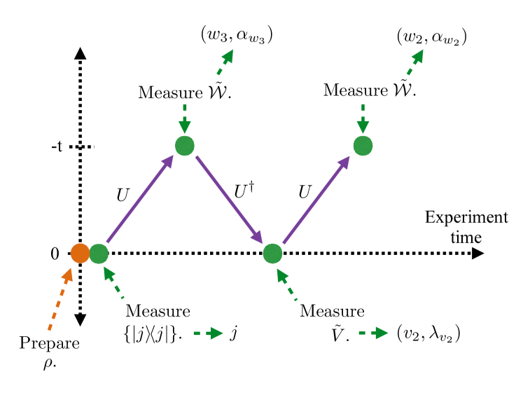
(b)

Figure 1: Quantum processes described by the complex amplitudes in the Jarzynski-like equality for the out-of-time-ordered correlator (OTOC): Theorem 1 shows that the OTOC depends on a complex distribution $P(W,W^{\prime})$. This $P(W,W^{\prime})$ parallels the probability distribution over possible values of thermodynamic work in Jarzynski’s Equality. $P(W,W^{\prime})$ results from summing products $A_{\rho}^{*}(.)A_{\rho}(.)$. Each $A_{\rho}(.)$ denotes a probability amplitude [Eq. (II.A)], so each product resembles a probability. But the amplitudes’ arguments differ, due to the OTOC’s out-of-time ordering: The amplitudes correspond to different quantum processes. Figure 1(a) illustrates the process associated with the $A_{\rho}^{*}(.)$; and Fig. 1(b), the process associated with the $A_{\rho}(.)$. Time runs from left to right. Each process begins with the preparation of the state $\rho=\sum_{j}p_{j}\lvert j\rangle\!\langle j\rvert$ and a measurement of the state’s eigenbasis. Three evolutions ($U$, $U^{\dagger}$, $U$) then alternate with three measurements of observables ($\tilde{\mathcal{W}}$, $\tilde{V}$, $\tilde{\mathcal{W}}$). If the initial state commutes with the Hamiltonian $H$ (e.g., if $\rho=e^{-H/T}/Z$), the first $U$ can be omitted. Figures 1(a) and 1(b) are used to define $P(W,W^{\prime})$, rather than illustrating protocols for measuring $P(W,W^{\prime})$. $P(W,W^{\prime})$ can be inferred from weak measurements and from interferometry.

II.B Combined quantum amplitude $\tilde{A}_{\rho}$

Combining quantum amplitudes $A_{\rho}$ yields a quantity $\tilde{A}_{\rho}$ that is nearly a probability but that differs due to the OTOC’s out-of-time ordering. I first define $\tilde{A}_{\rho}$, which resembles the Kirkwood-Dirac quasiprobability Kirkwood_33_Quantum ; Dirac_45_On ; Dressel_15_Weak ; BrianDisc . We gain insight into $\tilde{A}_{\rho}$ by supposing that $[\rho,\,\mathcal{W}]=0$, e.g., that $\rho$ is the infinite-temperature Gibbs state $\mathbbm{1}/d$. $\tilde{A}_{\rho}$ can reduce to a probability in this case, and protocols for measuring $\tilde{A}_{\rho}$ simplify. I introduce weak-measurement and interference schemes for inferring $\tilde{A}_{\rho}$ experimentally.

II.B.1 Definition of the combined quantum amplitude $\tilde{A}_{\rho}$

Consider measuring the probability amplitudes $A_{\rho}$ associated with all the possible measurement outcomes. Consider fixing an outcome septuple $(w_{2},\alpha_{w_{2}};v_{1},\lambda_{v_{1}};w_{1},\alpha_{w_{1}};j)$. The amplitude $A_{\rho}(w_{2},\alpha_{w_{2}};v_{1},\lambda_{v_{1}};w_{1},\alpha_{w_{1}};j)$ describes one realization, illustrated in Fig. 1(a), of the protocol $\mathcal{P}$. Call this realization $a$.

Consider the $\mathcal{P}$ realization, labeled $b$, illustrated in Fig. 1(b). The initial and final measurements yield the same outcomes as in $a$ [outcomes $j$ and $(w_{2},\alpha_{w_{2}})$]. Let $(w_{3},\alpha_{w_{3}})$ and $(v_{2},\lambda_{v_{2}})$ denote the outcomes of the second and third measurements in $b$. Realization $b$ corresponds to the probability amplitude $A_{\rho}(w_{2},\alpha_{w_{2}};v_{2},\lambda_{v_{2}};w_{3},\alpha_{w_{3}};j)$.

Let us complex-conjugate the $b$ amplitude and multiply by the $a$ amplitude. We marginalize over $j$ and over $(w_{1},\alpha_{w_{1}})$, forgetting about the corresponding measurement outcomes:

$$\tilde{A}_{\rho}(w,v,\alpha_{w},\lambda_{v}) :=\sum_{j,(w_{1},\alpha_{w_{1}})}A^{*}_{\rho}(w_{2},\alpha_{w_{2}};v_{2},\lambda_{v_{2}};w_{3},\alpha_{w_{3}};j)$$

$$\;\times A_{\rho}(w_{2},\alpha_{w_{2}};v_{1},\lambda_{v_{1}};w_{1},\alpha_{w_{1}};j)\,.$$ (3)

The shorthand $w$ encapsulates the list $(w_{1},w_{2})$. The shorthands $v$, $\alpha_{w}$ and $\lambda_{v}$ are defined analogously.

Let us substitute in from Eq. (II.A) and invoke $\langle A|B\rangle^{*}=\langle B|A\rangle$. The sum over $(w_{1},\alpha_{w_{1}})$ evaluates to a resolution of unity. The sum over $j$ evaluates to $\rho$:

$$\tilde{A}_{\rho}(w,v,\alpha_{w},\lambda_{v})=\langle w_{3},\alpha_{w_{3}}|U|v_{2},\lambda_{v_{2}}\rangle\langle v_{2},\lambda_{v_{2}}|U^{\dagger}|w_{2},\alpha_{w_{2}}\rangle$$

$$\qquad\times\langle w_{2},\alpha_{w_{2}}|U|v_{1},\lambda_{v_{1}}\rangle\langle v_{1},\lambda_{v_{1}}|\rho U^{\dagger}|w_{3},\alpha_{w_{3}}\rangle\,.$$ (4)

This $\tilde{A}_{\rho}$ resembles the Kirkwood-Dirac quasiprobability Dressel_15_Weak ; BrianDisc . Quasiprobabilities surface in quantum optics and quantum foundations Carmichael_02_Statistical ; Ferrie_11_Quasi . Quasiprobabilities generalize probabilities to quantum settings. Whereas probabilities remain between 0 and 1, quasiprobabilities can assume negative and nonreal values. Nonclassical values signal quantum phenomena such as entanglement. The best-known quasiprobabilities include the Wigner function, the Glauber-Sudarshan $P$ representation, and the Husimi $Q$ representation. Kirkwood and Dirac defined another quasiprobability in 1933 and in 1945 Kirkwood_33_Quantum ; Dirac_45_On . Interest in the Kirkwood-Dirac quasiprobability has revived recently. The distribution can assume nonreal values, obeys Bayesian updating, and has been measured experimentally Lundeen_11_Direct ; Lundeen_12_Procedure ; Bamber_14_Observing ; Mirhosseini_14_Compressive .

The Kirkwood-Dirac distribution for a state $\sigma\in\mathcal{D}(\mathcal{H})$ has the form $\langle f|a\rangle\langle a|\sigma|f\rangle$, wherein $\left\{\lvert f\rangle\!\langle f\rvert\right\}$ and $\left\{\lvert a\rangle\!\langle a\rvert\right\}$ denote bases for $\mathcal{H}$ Dressel_15_Weak . Equation (II.B.1) has the same form except contains more outer products. Marginalizing $\tilde{A}_{\rho}$ over every variable except one $w_{\ell}$ [or one $v_{\ell}$, one $(w_{\ell},\,\alpha_{w_{\ell}})$, or one $(v_{\ell},\,\lambda_{v_{\ell}})$] yields a probability, as does marginalizing the Kirkwood-Dirac distribution over every variable except one. The precise nature of the relationship between $\tilde{A}_{\rho}$ and the Kirkwood-Dirac quasiprobability is under investigation BrianDisc . For now, I harness the similarity to formulate a weak-measurement scheme for $\tilde{A}_{\rho}$ in Sec. II.B.3.

$\tilde{A}_{\rho}$ is nearly a probability: $\tilde{A}_{\rho}$ results from multiplying a complex-conjugated probability amplitude $A^{*}_{\rho}$ by a probability amplitude $A_{\rho}$. So does the quantum mechanical probability density $p(x)=\psi^{*}(x)\psi(x)$. Hence the quasiprobability resembles a probability. Yet the argument of the $\psi^{*}$ equals the argument of the $\psi$. The argument of the $A^{*}_{\rho}$ does not equal the argument of the $A_{\rho}$. This discrepancy stems from the OTOC’s out-of-time ordering. $\tilde{A}_{\rho}$ can be regarded as like a probability, differing due to the out-of-time ordering. $\tilde{A}_{\rho}$ reduces to a probability under conditions discussed in Sec. II.B.2. The reduction reinforces the parallel between Theorem 1 and the fluctuation-relation work TLH_07_Work , which involves a probability distribution that resembles $\tilde{A}_{\rho}$.

II.B.2 Simple case, reduction of $\tilde{A}_{\rho}$ to a probability

Suppose that $\rho$ shares the $\tilde{\mathcal{W}}(t)$ eigenbasis: $\rho=\rho_{\mathcal{W}(t)}:=\sum_{w_{\ell},\alpha_{w_{\ell}}}p_{w_{\ell},\alpha_{w_{\ell}}}U^{\dagger}\lvert w_{\ell},\alpha_{w_{\ell}}\rangle\!\langle w_{\ell},\alpha_{w_{\ell}}\rvert U$. For example, $\rho$ may be the infinite-temperature Gibbs state $\mathbbm{1}/d$. Equation (II.B.1) becomes

$$\tilde{A}_{\rho_{\mathcal{W}(t)}}(w,v,\alpha_{w},\lambda_{v})=\langle w_{3},\alpha_{w_{3}}|U|v_{2},\lambda_{v_{2}}\rangle$$

$$\qquad\times\langle v_{2},\lambda_{v_{2}}|U^{\dagger}|w_{2},\alpha_{w_{2}}\rangle\langle w_{2},\alpha_{w_{2}}|U|v_{1},\lambda_{v_{1}}\rangle$$

$$\qquad\times\langle v_{1},\lambda_{v_{1}}|U^{\dagger}|w_{3},\alpha_{w_{3}}\rangle\,p_{w_{3},\alpha_{w_{3}}}\,.$$ (5)

The weak-measurement protocol simplifies, as discussed in Sec. II.B.3.

Equation (II.B.2) reduces to a probability if $(w_{3},\alpha_{w_{3}})=(w_{2},\alpha_{w_{2}})$ or if $(v_{2},\lambda_{v_{2}})=(v_{1},\lambda_{v_{1}})$. For example, suppose that $(w_{3},\alpha_{w_{3}})=(w_{2},\alpha_{w_{2}})$:

$$\tilde{A}_{\rho_{\mathcal{W}(t)}}\bm{(}(w_{2},w_{2}),v,(\alpha_{w_{2}},\alpha_{w_{2}}),\lambda_{v}\bm{)}=|\langle v_{2},\lambda_{v_{2}}|U^{\dagger}|w_{2},\alpha_{w_{2}}\rangle|^{2}$$

$$\qquad\qquad\qquad\times|\langle v_{1},\lambda_{v_{1}}|U^{\dagger}|w_{2},\alpha_{w_{2}}\rangle|^{2}\,p_{w_{2},\alpha_{w_{2}}}$$ (6)

$$\qquad=p(v_{2},\lambda_{v_{2}}|w_{2},\alpha_{w_{2}})\,p(v_{1},\lambda_{v_{1}}|w_{2},\alpha_{w_{2}})\,p_{w_{2},\alpha_{w_{2}}}\,.$$ (7)

The $p_{w_{2},\alpha_{w_{2}}}$ denotes the probability that preparing $\rho$ and measuring $\tilde{\mathcal{W}}$ will yield $(w_{2},\alpha_{w_{2}})$. Each $p(v_{\ell},\lambda_{v_{\ell}}|w_{2},\alpha_{w_{2}})$ denotes the conditional probability that preparing $\lvert w_{2},\alpha_{w_{2}}\rangle$, backward-evolving under $U^{\dagger}$, and measuring $\tilde{V}$ will yield $(v_{\ell},\lambda_{v_{\ell}})$. Hence the combination $\tilde{A}_{\rho}$ of probability amplitudes is nearly a probability: $\tilde{A}_{\rho}$ reduces to a probability under simplifying conditions.

Equation (7) strengthens the analogy between Theorem 1 and the fluctuation relation in TLH_07_Work . Equation (10) in TLH_07_Work contains a conditional probability $p(m,t_{f}|n)$ multiplied by a probability $p_{n}$. These probabilities parallel the $p(v_{1},\lambda_{v_{1}}|w_{1},\alpha_{w_{1}})$ and $p_{w_{1},\alpha_{w_{1}}}$ in Eq. (7). Equation (7) contains another conditional probability, $p(v_{2},\lambda_{v_{2}}|w_{1},\alpha_{w_{1}})$, due to the OTOC’s out-of-time ordering.

II.B.3 Weak-measurement scheme for the combined quantum amplitude $\tilde{A}_{\rho}$

$\tilde{A}_{\rho}$ is related to the Kirkwood-Dirac quasiprobability, which has been inferred from weak measurements Dressel_14_Understanding ; Kofman_12_Nonperturbative ; Lundeen_11_Direct ; Lundeen_12_Procedure ; Bamber_14_Observing ; Mirhosseini_14_Compressive . I sketch a weak-measurement scheme for inferring $\tilde{A}_{\rho}$. Details appear in Appendix A.

Let $\mathcal{P}_{\rm weak}$ denote the following protocol:

1. Prepare $\rho$.

2. Couple the system’s $\tilde{V}$ weakly to an ancilla $\mathcal{A}_{a}$. Measure $\mathcal{A}_{a}$ strongly.

3. Evolve $S$ forward under $U$.

4. Couple the system’s $\tilde{\mathcal{W}}$ weakly to an ancilla $\mathcal{A}_{b}$. Measure $\mathcal{A}_{b}$ strongly.

5. Evolve $S$ backward under $U^{\dagger}$.

6. Couple the system’s $\tilde{V}$ weakly to an ancilla $\mathcal{A}_{c}$. Measure $\mathcal{A}_{c}$ strongly.

7. Evolve $S$ forward under $U$.

8. Measure $\tilde{\mathcal{W}}$ strongly (e.g., projectively).

Consider performing $\mathcal{P}_{\rm weak}$ many times. From the measurement statistics, one can infer the form of $\tilde{A}_{\rho}(w,v,\alpha_{w},\lambda_{v})$.

$\mathcal{P}_{\rm weak}$ offers an experimental challenge: Concatenating weak measurements raises the number of trials required to infer a quasiprobability. The challenge might be realizable with modifications to existing set-ups (e.g., White_16_Preserving ; Dressel_14_Implementing ). Additionally, $\mathcal{P}_{\rm weak}$ simplifies in the case discussed in Sec. II.B.2—if $\rho$ shares the $\tilde{\mathcal{W}}(t)$ eigenbasis, e.g., if $\rho=\mathbbm{1}/d$. The number of weak measurements reduces from three to two. Appendix A contains details.

II.B.4 Interference-based measurement of $\tilde{A}_{\rho}$

$\tilde{A}_{\rho}$ can be inferred not only from weak measurement, but also from interference. In certain cases—if $\rho$ shares neither the $\mathcal{W}$, the $\mathcal{W}(t)$, nor the $V$ eigenbasis—also quantum state tomography is needed. From interference, one infers the inner products $\langle a|\mathcal{U}|b\rangle$ in $\tilde{A}_{\rho}$. Eigenstates of $\tilde{\mathcal{W}}$ and $\tilde{V}$ are labeled by $a$ and $b$; and $\mathcal{U}=U,U^{\dagger}$. The matrix element $\langle v_{1},\lambda_{v_{1}}|\rho U^{\dagger}|w_{3},\alpha_{w_{3}}\rangle$ is inferred from quantum state tomography in certain cases.

The interference scheme proceeds as follows. An ancilla $\mathcal{A}$ is prepared in a superposition $\frac{1}{\sqrt{2}}\;(\lvert 0\rangle+\lvert 1\rangle)$. The system $S$ is prepared in a fiducial state $\lvert f\rangle$. The ancilla controls a conditional unitary on $S$: If $\mathcal{A}$ is in state $\lvert 0\rangle$, $S$ is rotated to $\mathcal{U}\lvert b\rangle$. If $\mathcal{A}$ is in $\lvert 1\rangle$, $S$ is rotated to $\lvert a\rangle$. The ancilla’s state is rotated about the $x$-axis [if the imaginary part $\Im(\langle a|\mathcal{U}|b\rangle)$ is being inferred] or about the $y$-axis [if the real part $\Re(\langle a|\mathcal{U}|b\rangle)$ is being inferred]. The ancilla’s $\sigma_{z}$ and the system’s $\left\{\lvert a\rangle\right\}$ are measured. The outcome probabilities imply the value of $\langle a|\mathcal{U}|b\rangle$. Details appear in Appendix B.

The time parameter $t$ need not be negated in any implementation of the protocol. The absence of time reversal has been regarded as beneficial in OTOC-measurement schemes Yao_16_Interferometric ; Zhu_16_Measurement , as time reversal can be difficult to implement.

Interference and weak measurement have been performed with cold atoms Smith_04_Continuous , which have been proposed as platforms for realizing scrambling and quantum chaos Swingle_16_Measuring ; Yao_16_Interferometric ; Danshita_16_Creating . Yet cold atoms are not necessary for measuring $\tilde{A}_{\rho}$. The measurement schemes in this paper are platform-nonspecific.

II.C Measurable random variables $W$ and $W^{\prime}$

The combined quantum amplitude $\tilde{A}_{\rho}$ is defined in terms of two realizations of the protocol $\mathcal{P}$. The realizations yield measurement outcomes $w_{2}$, $w_{3}$, $v_{1}$, and $v_{2}$. Consider complex-conjugating two outcomes: $w_{3}\mapsto w^{*}_{3}$, and $v_{2}\mapsto v^{*}_{2}$. The four values are combined into

$$W:=w_{3}^{*}v_{2}^{*}\quad\text{and}\quad W^{\prime}:=w_{2}v_{1}\,.$$ (8)

Suppose, for example, that $\mathcal{W}$ and $V$ denote single-qubit Paulis. $(W,W^{\prime})$ can equal $(1,1),(1,-1),(-1,1)$, or $(-1,-1)$. $W$ and $W^{\prime}$ function analogously to the thermodynamic work in Jarzynski’s Equality: $W$, $W^{\prime}$, and work are random variables calculable from measurement outcomes.

II.D Complex distribution function $P(W,W^{\prime})$

Jarzynski’s Equality depends on a probability distribution $P(W)$. I define an analog $P(W,W^{\prime})$ in terms of the combined quantum amplitude $\tilde{A}_{\rho}$.

Consider fixing $W$ and $W^{\prime}$. For example, let $(W,W^{\prime})=(1,-1)$. Consider the set of all possible outcome octuples $(w_{2},\alpha_{w_{2}};w_{3},\alpha_{w_{3}};v_{1},\lambda_{v_{1}};v_{2},\lambda_{v_{2}})$ that satisfy the constraints $W=w_{3}^{*}v_{2}^{*}$ and $W^{\prime}=w_{2}v_{1}$. Each octuple corresponds to a set of combined quantum amplitudes $\tilde{A}_{\rho}(w,v,\alpha_{w},\lambda_{v})$. These $\tilde{A}_{\rho}$’s are summed, subject to the constraints:

$$P(W,W^{\prime}) :=\sum_{w,v,\alpha_{w},\lambda_{v}}\tilde{A}_{\rho}(w,v,\alpha_{w},\lambda_{v})$$

$$\qquad\times\delta_{W(w_{3}^{*}v_{2}^{*})}\,\delta_{W^{\prime}(w_{2}v_{1})}\,.$$ (9)

The Kronecker delta is denoted by $\delta_{ab}$.

The form of Eq. (II.D) is analogous to the form of the $P(W)$ in TLH_07_Work [Eq. (10)], as $\tilde{A}_{\rho}$ is nearly a probability. Equation (II.D), however, encodes interference of quantum probability amplitudes.

$P(W,W^{\prime})$ resembles a joint probability distribution. Summing any function $f(W,W^{\prime})$ with weights $P(W,W^{\prime})$ yields the average-like quantity

$$\left\langle f(W,W^{\prime})\right\rangle:=\sum_{W,W^{\prime}}f(W,W^{\prime})\,P(W,W^{\prime})\,.$$ (10)

III Result

The above definitions feature in the Jarzynski-like equality for the OTOC.

Theorem 1.

The out-of-time-ordered correlator obeys the Jarzynski-like equality

$$F(t)=\frac{\partial^{2}}{\partial\beta\,\partial\beta^{\prime}}\>\left\langle e^{-(\beta W+\beta^{\prime}W^{\prime})}\right\rangle\Big{\lvert}_{\beta,\beta^{\prime}=0}\,,$$ (11)

wherein $\beta,\beta^{\prime}\in\mathbb{R}$.

Proof.

The derivation of Eq. (11) is inspired by TLH_07_Work . Talkner et al. cast Jarzynski’s Equality in terms of a time-ordered correlator of two exponentiated Hamiltonians. Those authors invoke the characteristic function

$$\mathcal{G}(s):=\int dW\;e^{isW}\,P(W)\,,$$ (12)

the Fourier transform of the probability distribution $P(W)$. The integration variable $s$ is regarded as an imaginary inverse temperature: $is=-\beta$. We analogously invoke the (discrete) Fourier transform of $P(W,W^{\prime})$:

$$\mathcal{G}(s,s^{\prime}):=\sum_{W}e^{isW}\sum_{W^{\prime}}e^{is^{\prime}W^{\prime}}P(W,W^{\prime})\,,$$ (13)

wherein $is=-\beta$ and $is^{\prime}=-\beta^{\prime}$.

$P(W,W^{\prime})$ is substituted in from Eqs. (II.D) and (II.B.1). The delta functions are summed over:

$$\mathcal{G}(s,s^{\prime})=\sum_{w,v,\alpha_{w},\lambda_{v}}e^{isw_{3}^{*}v_{2}^{*}}\>e^{is^{\prime}w_{2}v_{1}}\>\langle w_{3},\alpha_{w_{3}}|U|v_{2},\lambda_{v_{2}}\rangle$$

$$\qquad\times\langle v_{2},\lambda_{v_{2}}|U^{\dagger}|w_{2},\alpha_{w_{2}}\rangle\langle w_{2},\alpha_{w_{2}}|U|v_{1},\lambda_{v_{1}}\rangle$$

$$\qquad\times\langle v_{1},\lambda_{v_{1}}|U^{\dagger}\rho(t)|w_{3},\alpha_{w_{3}}\rangle\,.$$ (14)

The $\rho U^{\dagger}$ in Eq. (II.B.1) has been replaced with $U^{\dagger}\rho(t)$, wherein $\rho(t):=U\rho U^{\dagger}$.

The sum over $(w_{3},\alpha_{w_{3}})$ is recast as a trace. Under the trace’s protection, $\rho(t)$ is shifted to the argument’s left-hand side. The other sums and the exponentials are distributed across the product:

$$\mathcal{G} (s,s^{\prime})={\rm Tr}\Bigg{(}\rho(t)\Bigg{[}\sum_{w_{3},\alpha_{w_{3}}}\lvert w_{3},\alpha_{w_{3}}\rangle\!\langle w_{3},\alpha_{w_{3}}\rvert$$

$$\qquad\times U\sum_{v_{2},\lambda_{v_{2}}}e^{is{{w_{3}}^{*}}v_{2}^{*}}\lvert v_{2},\lambda_{v_{2}}\rangle\!\langle v_{2},\lambda_{v_{2}}\rvert U^{\dagger}\Bigg{]}$$

$$\times\Bigg{[}\sum_{w_{2},\alpha_{w_{2}}}\lvert w_{2},\alpha_{w_{2}}\rangle\!\langle w_{2},\alpha_{w_{2}}\rvert$$

$$\qquad\times U\sum_{v_{1},\lambda_{v_{1}}}e^{is^{\prime}w_{2}v_{1}}\lvert v_{1},\lambda_{v_{1}}\rangle\!\langle v_{1},\lambda_{v_{1}}\rvert\,U^{\dagger}\Bigg{]}\Bigg{)}\,.$$ (15)

The $v_{\ell}$ and $\lambda_{v_{\ell}}$ sums are eigendecompositions of exponentials of unitaries:

$$\mathcal{G} (s,s^{\prime})={\rm Tr}\Bigg{(}\rho(t)\Bigg{[}\sum_{w_{3},\alpha_{w_{3}}}\lvert w_{3},\alpha_{w_{3}}\rangle\!\langle w_{3},\alpha_{w_{3}}\rvert U\,e^{isw_{3}^{*}V^{\dagger}}\,U^{\dagger}\Bigg{]}$$

$$\qquad\times\Bigg{[}\sum_{w_{2},\alpha_{w_{2}}}\lvert w_{2},\alpha_{w_{2}}\rangle\!\langle w_{2},\alpha_{w_{2}}\rvert U\,e^{is^{\prime}w_{2}V}\,U^{\dagger}\Bigg{]}\Bigg{)}\,.$$ (16)

The unitaries time-evolve the $V$’s:

$$\mathcal{G} (s,s^{\prime})={\rm Tr}\Bigg{(}\rho(t)\Bigg{[}\sum_{w_{3},\alpha_{w_{3}}}\lvert w_{3},\alpha_{w_{3}}\rangle\!\langle w_{3},\alpha_{w_{3}}\rvert e^{isw_{2}^{*}V^{\dagger}(-t)}\Bigg{]}$$

$$\qquad\times\Bigg{[}\sum_{w_{2},\alpha_{w_{2}}}\lvert w_{2},\alpha_{w_{2}}\rangle\!\langle w_{2},\alpha_{w_{2}}\rvert e^{is^{\prime}w_{2}V(-t)}\Bigg{]}\Bigg{)}\,.$$ (17)

We differentiate with respect to $is^{\prime}=-\beta^{\prime}$ and with respect to $is=-\beta$. Then, we take the limit as $\beta,\beta^{\prime}\to 0$:

$$\frac{\partial^{2}}{\partial\beta\,\partial\beta^{\prime}}\mathcal{G}\left(i\beta,i\beta^{\prime}\right)\Big{\lvert}_{\beta,\beta^{\prime}=0}$$ (18)

$$={\rm Tr}\Bigg{(}\rho(t)\Bigg{[}\sum_{w_{3},\alpha_{w_{3}}}w_{3}^{*}\lvert w_{3},\alpha_{w_{3}}\rangle\!\langle w_{3},\alpha_{w_{3}}\rvert V^{\dagger}(-t)\Bigg{]}$$ (19)

$$\qquad\qquad\times\Bigg{[}\sum_{w_{2},\alpha_{w_{2}}}w_{2}\lvert w_{2},\alpha_{w_{2}}\rangle\!\langle w_{2},\alpha_{w_{2}}\rvert V(-t)\Bigg{]}\Bigg{)}$$

$$={\rm Tr}\bm{(}\rho(t)\,\mathcal{W}^{\dagger}\,V^{\dagger}(-t)\,\mathcal{W}\,V(-t)\bm{)}\,.$$ (20)

Recall that $\rho(t):=U\rho U^{\dagger}$. Time dependence is transferred from $\rho(t)$, $V(-t)=UV^{\dagger}U^{\dagger}$, and $V^{\dagger}(t)=UVU^{\dagger}$ to $\mathcal{W}^{\dagger}$ and $\mathcal{W}$, under the trace’s cyclicality:

$$\frac{\partial^{2}}{\partial\beta\,\partial\beta^{\prime}}\mathcal{G}(i\beta,i\beta^{\prime})\Big{\lvert}_{\beta,\beta^{\prime}=0}={\rm Tr}\left(\rho\,\mathcal{W}^{\dagger}(t)\,V^{\dagger}\,\mathcal{W}(t)\,V\right)$$ (21)

$$\qquad\qquad\qquad\qquad=\left\langle\mathcal{W}^{\dagger}(t)\,V^{\dagger}\,\mathcal{W}(t)\,V\right\rangle=F(t)\,.$$ (22)

By Eqs. (10) and (13), the left-hand side equals

$$\frac{\partial^{2}}{\partial\beta\,\partial\beta^{\prime}}\left\langle e^{-(\beta W+\beta^{\prime}W^{\prime})}\right\rangle\Big{\lvert}_{\beta,\beta^{\prime}=0}\,.$$ (23)

∎

Theorem 1 resembles Jarzynski’s fluctuation relation in several ways. Jarzynski’s Equality encodes a scheme for measuring the difficult-to-calculate $\Delta F$ from realizable nonequilibrium trials. Theorem 1 encodes a scheme for measuring the difficult-to-calculate $F(t)$ from realizable nonequilibrium trials. $\Delta F$ depends on just a temperature and two Hamiltonians. Similarly, the conventional $F(t)$ (defined with respect to $\rho=e^{-H/T}/Z$) depends on just a temperature, a Hamiltonian, and two unitaries. Jarzynski relates $\Delta F$ to the characteristic function of a probability distribution. Theorem 1 relates $F(t)$ to (a moment of) the characteristic function of a (complex) distribution.

The complex distribution, $P(W,W^{\prime})$, is a combination of probability amplitudes $\tilde{A}_{\rho}$ related to quasiprobabilities. The distribution in Jarzynski’s Equality is a combination of probabilities. The quasiprobability-vs.-probability contrast fittingly arises from the OTOC’s out-of-time ordering. $F(t)$ signals quantum behavior (noncommutation), as quasiprobabilities signal quantum behaviors (e.g., entanglement). Time-ordered correlators similar to $F(t)$ track only classical behaviors and are moments of (summed) classical probabilities BrianDisc . OTOCs that encode more time reversals than $F(t)$ are moments of combined quasiprobability-like distributions lengthier than $\tilde{A}_{\rho}$ BrianDisc .

IV Conclusions

The Jarzynski-like equality for the out-of-time correlator combines an important tool from nonequilibrium statistical mechanics with an important tool from quantum information, high-energy theory, and condensed matter. The union opens all these fields to new modes of analysis.

For example, Theorem 1 relates the OTOC to a combined quantum amplitude $\tilde{A}_{\rho}$. This $\tilde{A}_{\rho}$ is closely related to a quasiprobability. The OTOC and quasiprobabilities have signaled nonclassical behaviors in distinct settings—in high-energy theory and condensed matter and in quantum optics, respectively. The relationship between OTOCs and quasiprobabilities merits study: What is the relationship’s precise nature? How does $\tilde{A}_{\rho}$ behave over time scales during which $F(t)$ exhibits known behaviors (e.g., until the dissipation time or from the dissipation time to the scrambling time Swingle_16_Measuring )? Under what conditions does $\tilde{A}_{\rho}$ behave nonclassically (assume negative or nonreal values)? How does a chaotic system’s $\tilde{A}_{\rho}$ look? These questions are under investigation BrianDisc .

As another example, fluctuation relations have been used to estimate the free-energy difference $\Delta F$ from experimental data. Experimental measurements of $F(t)$ are possible for certain platforms, in certain regimes Swingle_16_Measuring ; Yao_16_Interferometric ; Zhu_16_Measurement ; Li_16_Measuring ; Garttner_16_Measuring . Theorem 1 expands the set of platforms and regimes. Measuring quantum amplitudes, as via weak measurements Lundeen_11_Direct ; Lundeen_12_Procedure ; Bamber_14_Observing ; Mirhosseini_14_Compressive , now offers access to $F(t)$. Inferring small systems’ $\tilde{A}_{\rho}$’s with existing platforms White_16_Preserving might offer a challenge for the near future.

Finally, Theorem 1 can provide a new route to bounding $F(t)$. A Lyapunov exponent $\lambda_{\rm L}$ governs the chaotic decay of $F(t)$. The exponent has been bounded, including with Lieb-Robinson bounds and complex analysis Maldacena_15_Bound ; Lashkari_13_Towards ; Kitaev_15_Simple . The right-hand side of Eq. (11) can provide an independent bounding method that offers new insights.

Appendix A Weak measurement of the combined quantum amplitude $\tilde{A}_{\rho}$

$\tilde{A}_{\rho}$ [Eq. (II.B.1)] resembles the Kirkwood-Dirac quasiprobability for a quantum state Kirkwood_33_Quantum ; Dirac_45_On ; Dressel_15_Weak . This quasiprobability has been inferred from weak-measurement experiments Lundeen_11_Direct ; Lundeen_12_Procedure ; Bamber_14_Observing ; Mirhosseini_14_Compressive ; Dressel_14_Understanding . Weak measurements have been performed on cold atoms Smith_04_Continuous , which have been proposed as platforms for realizing scrambling and quantum chaos Swingle_16_Measuring ; Yao_16_Interferometric ; Danshita_16_Creating .

$\tilde{A}_{\rho}$ can be inferred from many instances of a protocol $\mathcal{P}_{\rm weak}$. $\mathcal{P}_{\rm weak}$ consists of a state preparation, three evolutions interleaved with three weak measurements, and a strong measurement. The steps appear in Sec. II.B.3.

I here flesh out the protocol, assuming that the system, $S$, begins in the infinite-temperature Gibbs state: $\rho=\mathbbm{1}/d$. $\tilde{A}_{\rho}$ simplifies as in Eq. (II.B.2). The final factor becomes $p_{w_{3},\alpha_{w_{3}}}=1/d$. The number of weak measurements in $\mathcal{P}_{\rm weak}$ reduces to two. Generalizing to arbitrary $\rho$’s is straightforward but requires lengthier calculations and more “background” terms.

Each trial in the simplified $\mathcal{P}_{\rm weak}$ consists of a state preparation, three evolutions interleaved with two weak measurements, and a strong measurement. Loosely, one performs the following protocol: Prepare $\lvert w_{3},\alpha_{w_{3}}\rangle$. Evolve $S$ backward under $U^{\dagger}$. Measure $\lvert v_{1},\lambda_{v_{1}}\rangle\!\langle v_{1},\lambda_{v_{1}}\rvert$ weakly. Evolve $S$ forward under $U$. Measure $\lvert w_{2},\alpha_{w_{2}}\rangle\!\langle w_{2},\alpha_{w_{2}}\rvert$ weakly. Evolve $S$ backward under $U^{\dagger}$. Measure $\lvert v_{2},\lambda_{v_{2}}\rangle\!\langle v_{2},\lambda_{v_{2}}\rvert$ strongly.

Let us analyze the protocol in greater detail. The $\lvert w_{3},\alpha_{w_{3}}\rangle$ preparation and backward evolution yield $\lvert\psi\rangle=U^{\dagger}\lvert w_{3},\alpha_{w_{3}}\rangle$. The weak measurement of $\lvert v_{1},\lambda_{v_{1}}\rangle\!\langle v_{1},\lambda_{v_{1}}\rvert$ is implemented as follows: $S$ is coupled weakly to an ancilla $\mathcal{A}_{a}$. The observable $\tilde{V}$ of $S$ comes to be correlated with an observable of $\mathcal{A}_{a}$. Example $\mathcal{A}_{a}$ observables include a pointer’s position on a dial and a component $\sigma_{\ell}$ of a qubit’s spin (wherein $\ell=x,y,z$). The $\mathcal{A}_{a}$ observable is measured projectively. Let $x$ denote the measurement’s outcome. $x$ encodes partial information about the system’s state. We label by $(v_{1},\lambda_{v_{1}})$ the $\tilde{V}$ eigenvalue most reasonably attributable to $S$ if the $\mathcal{A}_{a}$ measurement yields $x$.

The coupling and the $\mathcal{A}_{a}$ measurement evolve $\lvert\psi\rangle$ under the Kraus operator NielsenC10

$$M_{x}=\sqrt{p_{a}(x)}\>\mathbbm{1}+g_{a}(x)\,\lvert v_{1},\lambda_{v_{1}}\rangle\!\langle v_{1},\lambda_{v_{1}}\rvert\,.$$ (A1)

Equation (A1) can be derived, e.g., from the Gaussian-meter model Dressel_15_Weak ; Aharonov_88_How or the qubit-meter model White_16_Preserving . The projector can be generalized to a projector $\Pi_{v_{1}}$ onto a degenerate eigensubspace. The generalization may decrease exponentially the number of trials required BrianDisc . By the probabilistic interpretation of quantum channels, the baseline probability $p_{a}(x)$ denotes the likelihood that, in any given trial, $S$ fails to couple to $\mathcal{A}_{a}$ but the $\mathcal{A}_{a}$ measurement yields $x$ nonetheless. The detector is assumed, for convenience, to be calibrated such that

$$\int dx\cdot x\>p_{a}(x)=0\,.$$ (A2)

The small tunable parameter $g_{a}(x)$ quantifies the coupling strength.

The system’s state becomes $\lvert\psi^{\prime}\rangle=M_{x}U^{\dagger}\lvert w_{3},\alpha_{w_{3}}\rangle$, to within a normalization factor. $S$ evolves under $U$ as

$$\lvert\psi^{\prime}\rangle\mapsto\lvert\psi^{\prime\prime}\rangle=UM_{x}U^{\dagger}\lvert w_{3},\alpha_{w_{3}}\rangle\,,$$ (A3)

to within normalization. $\lvert w_{2},\alpha_{w_{2}}\rangle\!\langle w_{2},\alpha_{w_{2}}\rvert$ is measured weakly: $S$ is coupled weakly to an ancilla $\mathcal{A}_{b}$. $\tilde{\mathcal{W}}$ comes to be correlated with a pointer-like variable of $\mathcal{A}_{b}$. The pointer-like variable is measured projectively. Let $y$ denote the outcome. The coupling and measurement evolve $\lvert\psi^{\prime\prime}\rangle$ under the Kraus operator

$$M_{y}=\sqrt{p_{b}(y)}\>\mathbbm{1}+g_{b}(y)\,\lvert w_{2},\alpha_{w_{2}}\rangle\!\langle w_{2},\alpha_{w_{2}}\rvert\,.$$ (A4)

The system’s state becomes $\lvert\psi^{\prime\prime\prime}\rangle=M_{y}UM_{x}U^{\dagger}\lvert w_{3},\alpha_{w_{3}}\rangle$, to within normalization. The state evolves backward under $U^{\dagger}$. Finally, $\tilde{V}$ is measured projectively.

Each trial involves two weak measurements and one strong measurement. The probability that the measurements yield the outcomes $x$, $y$, and $(v_{2},\lambda_{v_{2}})$ is

$$\mathscr{P}_{\rm weak}\bm{(}x,y,(v_{2},\lambda_{v_{2}})\bm{)}=|\langle v_{2},\lambda_{v_{2}}|U^{\dagger}M_{y}UM_{x}U^{\dagger}|w_{3},\alpha_{w_{3}}\rangle|^{2}\,.$$ (A5)

Integrating over $x$ and $y$ yields

$$\mathcal{I}:=\int dx\;dy\cdot x\,y\;\mathscr{P}_{\rm weak}\bm{(}x,y,(v_{2},\lambda_{v_{2}})\bm{)}\,.$$ (A6)

We substitute in for $M_{x}$ and $M_{y}$ from Eqs. (A1) and (A4), then multiply out. We approximate to second order in the weak-coupling parameters. The calibration condition (A2) causes terms to vanish:

$$\mathcal{I} =\int dx\;dy\cdot x\>y\;\sqrt{p_{a}(x)\>p_{b}(y)}\Big{[}g_{a}(x)\,g_{b}(y)\cdot d$$

$$\times\tilde{A}_{\mathbbm{1}/d}(w,v,\alpha_{w},\lambda_{v})+{\rm c.c.}\Big{]}+\int dx\;dy\cdot x\>y\;\sqrt{p_{a}(x)\>p_{b}(y)}$$

$$\times\Big{[}g_{a}^{*}(x)\,g_{b}(y)\,\langle v_{2},\lambda_{v_{2}}|U^{\dagger}|w_{2},\alpha_{w_{2}}\rangle\langle w_{2},\alpha_{w_{2}}|w_{3},\alpha_{w_{3}}\rangle$$

$$\times\bm{(}\langle v_{2},\lambda_{v_{2}}|v_{1},\lambda_{v_{1}}\rangle\langle v_{1},\lambda_{v_{1}}|U^{\dagger}|w_{3},\alpha_{w_{3}}\rangle\bm{)}^{*}+{\rm c.c.}\Big{]}$$

$$+O\bm{(}g_{a}(x)^{2}\,g_{b}(y)\bm{)}+O\bm{(}g_{a}(x)\,g_{b}(y)^{2}\bm{)}\,.$$ (A7)

The baseline probabilities $p_{a}(x)$ and $p_{b}(x)$ are measured during calibration. Let us focus on the second integral. By orthonormality, $\langle w_{2},\alpha_{w_{2}}|w_{3},\alpha_{w_{3}}\rangle=\delta_{w_{2}w_{3}}\,\delta_{\alpha_{w_{2}}\alpha_{w_{3}}}$, and $\langle v_{2},\lambda_{v_{2}}|v_{1},\lambda_{v_{1}}\rangle=\delta_{v_{2}v_{1}}\,\delta_{\lambda_{v_{2}}\lambda_{v_{1}}}$. The integral vanishes if $(w_{3},\alpha_{w_{3}})\neq(w_{2},\alpha_{w_{2}})$ or if $(v_{2},\lambda_{v_{2}})\neq(v_{1},\lambda_{v_{1}})$. Suppose that $(w_{3},\alpha_{w_{3}})=(w_{2},\alpha_{w_{2}})$ and $(v_{2},\lambda_{v_{2}})=(v_{1},\lambda_{v_{1}})$. The second integral becomes

$$\int dx\;dy\cdot x\>y\;\sqrt{p_{a}(x)\,p_{b}(y)}\>\Big{[}g_{a}^{*}(x)\,g_{b}(y)\,$$

$$\qquad\times|\langle v_{2},\lambda_{v_{2}}|U^{\dagger}|w_{3},\alpha_{w_{3}}\rangle|^{2}+{\rm c.c.}\Big{]}.$$ (A8)

The square modulus, a probability, can be measured via Born’s rule. The experimenter controls $g_{a}(x)$ and $g_{b}(y)$. The second integral in Eq. (A) is therefore known.

From the first integral, we infer about $\tilde{A}_{\mathbbm{1}/d}$. Consider trials in which the couplings are chosen such that

$$\alpha:=\int dx\;dy\cdot x\>y\;\sqrt{p_{a}(x)\,p_{b}(y)}\>g_{a}(x)\,g_{b}(y)\in\mathbb{R}\,.$$ (A9)

The first integral becomes $2\alpha\,d\,\Re\bm{(}\tilde{A}_{\mathbbm{1}/d}(w,v,\alpha_{w},\lambda_{v})\bm{)}$. From these trials, one infers the real part of $\tilde{A}_{\mathbbm{1}/d}$. Now, consider trials in which $i\,\alpha\in\mathbb{R}$. The first bracketed term becomes $2|\alpha|\,d\,\Im\bm{(}\tilde{A}_{\mathbbm{1}/d}(w,v,\alpha_{w},\lambda_{v})\bm{)}\,.$ From these trials, one infers the imaginary part of $\tilde{A}_{\mathbbm{1}/d}$.

$\alpha$ can be tuned between real and imaginary in practice Lundeen_11_Direct . Consider a weak measurement in which the ancillas are qubits. An ancilla’s $\sigma_{y}$ can be coupled to a system observable. Whether the ancilla’s $\sigma_{x}$ or $\sigma_{y}$ is measured dictates whether $\alpha$ is real or imaginary.

The combined quantum amplitude $\tilde{A}_{\rho}$ can therefore be inferred from weak measurements. $\tilde{A}_{\rho}$ can be measured alternatively via interference.

Appendix B Interference-based measurement of the combined quantum amplitude $\tilde{A}_{\rho}$

I detail an interference-based scheme for measuring $\tilde{A}_{\rho}(w,v,\alpha_{w},\lambda_{v})$ [Eq. (II.B.1)]. The scheme requires no reversal of the time evolution in any trial. As implementing time reversal can be difficult, the absence of time reversal can benefit OTOC-measurement schemes Yao_16_Interferometric ; Zhu_16_Measurement .

I specify how to measure an inner product $z:=\langle a|\mathcal{U}|b\rangle$, wherein $a,b\in\{(w_{\ell},\alpha_{w_{\ell}}),(v_{m},\lambda_{v_{m}})\}$ and $\mathcal{U}\in\{U,U^{\dagger}\}$. Then, I discuss measurements of the state-dependent factor in Eq. (II.B.1).

The inner product $z$ is measured as follows. The system $S$ is initialized to some fiducial state $\lvert f\rangle$. An ancilla qubit $\mathcal{A}$ is prepared in the state $\frac{1}{\sqrt{2}}(\lvert 0\rangle+\lvert 1\rangle)$. The $+1$ and $-1$ eigenstates of $\sigma_{z}$ are denoted by $\lvert 0\rangle$ and $\lvert 1\rangle$. The composite system $\mathcal{A}S$ begins in the state $\lvert\psi\rangle=\frac{1}{\sqrt{2}}(\lvert 0\rangle\lvert f\rangle+\lvert 1\rangle\lvert f\rangle)$.

A unitary is performed on $S$, conditioned on $\mathcal{A}$: If $\mathcal{A}$ is in state $\lvert 0\rangle$, then $S$ is brought to state $\lvert b\rangle$, and $\mathcal{U}$ is applied to $S$. If $\mathcal{A}$ is in state $\lvert 1\rangle$, $S$ is brought to state $\lvert a\rangle$. The global state becomes $\lvert\psi^{\prime}\rangle=\frac{1}{\sqrt{2}}[\lvert 0\rangle(\mathcal{U}\lvert b\rangle)+\lvert 1\rangle\lvert a\rangle)]\,.$ A unitary $e^{-i\theta\sigma_{x}}$ rotates the ancilla’s state through an angle $\theta$ about the $x$-axis. The global state becomes

$$\lvert\psi^{\prime\prime}\rangle =\frac{1}{\sqrt{2}}\Bigg{[}\left(\cos\frac{\theta}{2}\lvert 0\rangle-i\sin\frac{\theta}{2}\lvert 1\rangle\right)(\mathcal{U}\lvert b\rangle)$$

$$\qquad+\left(-i\sin\frac{\theta}{2}\lvert 0\rangle+\cos\frac{\theta}{2}\lvert 1\rangle\right)\lvert a\rangle\Bigg{]}\,.$$ (B1)

The ancilla’s $\sigma_{z}$ is measured, and the system’s $\{\lvert a\rangle\}$ is measured. The probability that the measurements yield $+1$ and $a$ is

$$\mathscr{P}(+1,a) =\frac{1}{4}(1-\sin\theta)\Bigg{(}\cos^{2}\frac{\theta}{2}\>|z|^{2}-\sin\theta\>\Im(z)+\sin^{2}\frac{\theta}{2}\Bigg{)}\,.$$ (B2)

The imaginary part of $z$ is denoted by $\Im(z)$. $\mathscr{P}(+1,a)$ can be inferred from the outcomes of multiple trials. The $|z|^{2}$, representing a probability, can be measured independently. From the $|z|^{2}$ and $\mathscr{P}(+1,a)$ measurements, $\Im(z)$ can be inferred.

$\Re(z)$ can be inferred from another set of interference experiments. The rotation about $\hat{x}$ is replaced with a rotation about $\hat{y}$. The unitary $e^{-i\phi\sigma_{y}}$ implements this rotation, through an angle $\phi$. Equation (B) becomes

$$\lvert\tilde{\psi}^{\prime\prime}\rangle =\frac{1}{\sqrt{2}}\Big{[}\left(\cos\frac{\phi}{2}\,\lvert 0\rangle+\sin\frac{\phi}{2}\,\lvert 1\rangle\right)(\mathcal{U}\,\lvert b\rangle)$$

$$\qquad\qquad+\left(-\sin\frac{\phi}{2}\,\lvert 0\rangle+\cos\frac{\phi}{2}\,\lvert 1\rangle\right)\lvert a\rangle\Big{]}\,.$$ (B3)

The ancilla’s $\sigma_{z}$ and the system’s $\{\lvert a\rangle\}$ are measured. The probability that the measurements yield $+1$ and $a$ is

$$\tilde{\mathscr{P}}(+1,a) =\frac{1}{4}(1-\sin\phi)\Bigg{(}\cos^{2}\frac{\phi}{2}\,|z|^{2}$$

$$\qquad-\sin\phi\;\Re(z)+\sin^{2}\frac{\phi}{2}\Bigg{)}\,.$$ (B4)

One measures $\tilde{\mathscr{P}}(+1,a)$ and $|z|^{2}$, then infers $\Re(z)$. The real and imaginary parts of $z$ are thereby gleaned from interferometry.

Equation (II.B.1) contains the state-dependent factor $M:=\langle v_{1},\lambda_{v_{1}}|\rho U^{\dagger}|w_{3},\alpha_{w_{3}}\rangle$. This factor is measured easily if $\rho$ shares its eigenbasis with $\tilde{\mathcal{W}}(t)$ or with $\tilde{V}$. In these cases, $M$ assumes the form $\langle a|U^{\dagger}|b\rangle\,p$. The inner product is measured as above. The probability $p$ is measured via Born’s rule. In an important subcase, $\rho$ is the infinite-temperature Gibbs state $\mathbbm{1}/d$. The system’s size sets $p=1/d$. Outside of these cases, $M$ can be inferred from quantum tomography Paris_04_Q_State_Estimation . Tomography requires many trials but is possible in principle and can be realized with small systems.

References

• (1) S. H. Shenker and D. Stanford, Journal of High Energy Physics 3, 67 (2014).
• (2) S. H. Shenker and D. Stanford, Journal of High Energy Physics 12, 46 (2014).
• (3) S. H. Shenker and D. Stanford, Journal of High Energy Physics 5, 132 (2015).
• (4) D. A. Roberts, D. Stanford, and L. Susskind, Journal of High Energy Physics 3, 51 (2015).
• (5) D. A. Roberts and D. Stanford, Physical Review Letters 115, 131603 (2015).
• (6) J. Maldacena, S. H. Shenker, and D. Stanford, ArXiv e-prints (2015), 1503.01409.
• (7) A. Larkin and Y. N. Ovchinnikov, Soviet Journal of Experimental and Theoretical Physics 28 (1969).
• (8) Y. Sekino and L. Susskind, Journal of High Energy Physics 2008, 065 (2008).
• (9) Y. Huang, Y.-L. Zhang, and X. Chen, ArXiv e-prints (2016), 1608.01091.
• (10) B. Swingle and D. Chowdhury, ArXiv e-prints (2016), 1608.03280.
• (11) R. Fan, P. Zhang, H. Shen, and H. Zhai, ArXiv e-prints (2016), 1608.01914.
• (12) R.-Q. He and Z.-Y. Lu, ArXiv e-prints (2016), 1608.03586.
• (13) Y. Chen, ArXiv e-prints (2016), 1608.02765.
• (14) P. Hosur, X.-L. Qi, D. A. Roberts, and B. Yoshida, Journal of High Energy Physics 2, 4 (2016), 1511.04021.
• (15) B. Swingle, G. Bentsen, M. Schleier-Smith, and P. Hayden, ArXiv e-prints (2016), 1602.06271.
• (16) N. Y. Yao et al., ArXiv e-prints (2016), 1607.01801.
• (17) G. Zhu, M. Hafezi, and T. Grover, ArXiv e-prints (2016), 1607.00079.
• (18) J. Li et al., ArXiv e-prints (2016), 1609.01246.
• (19) M. Gärttner et al., ArXiv e-prints (2016), 1608.08938.
• (20) J. Maldacena and D. Stanford, ArXiv e-prints (2016), 1604.07818.
• (21) J. Polchinski and V. Rosenhaus, Journal of High Energy Physics 4, 1 (2016), 1601.06768.
• (22) C. Jarzynski, Physical Review Letters 78, 2690 (1997).
• (23) G. E. Crooks, Physical Review E 60, 2721 (1999).
• (24) H. Tasaki, arXiv e-print (2000), cond-mat/0009244.
• (25) J. Kurchan, eprint arXiv:cond-mat/0007360 (2000), cond-mat/0007360.
• (26) O.-P. Saira et al., Phys. Rev. Lett. 109, 180601 (2012).
• (27) C. Chipot and A. Pohorille, editors, Free Energy Calculations: Theory and Applications in Chemistry and Biology, Springer Series in Chemical Physics Vol. 86 (Springer-Verlag, 2007).
• (28) D. Collin et al., Nature 437, 231 (2005).
• (29) F. Douarche, S. Ciliberto, A. Petrosyan, and I. Rabbiosi, EPL (Europhysics Letters) 70, 593 (2005).
• (30) V. Blickle, T. Speck, L. Helden, U. Seifert, and C. Bechinger, Phys. Rev. Lett. 96, 070603 (2006).
• (31) N. C. Harris, Y. Song, and C.-H. Kiang, Phys. Rev. Lett. 99, 068101 (2007).
• (32) A. Mossa, M. Manosas, N. Forns, J. M. Huguet, and F. Ritort, Journal of Statistical Mechanics: Theory and Experiment 2009, P02060 (2009).
• (33) M. Manosas, A. Mossa, N. Forns, J. M. Huguet, and F. Ritort, Journal of Statistical Mechanics: Theory and Experiment 2009, P02061 (2009).
• (34) T. B. Batalhão et al., Physical Review Letters 113, 140601 (2014), 1308.3241.
• (35) S. An et al., Nature Physics 11, 193 (2015).
• (36) K. Maruyama, F. Nori, and V. Vedral, Rev. Mod. Phys. 81, 1 (2009).
• (37) J. Åberg, Nature Communications 4, 1925 (2013), 1110.6121.
• (38) N. Yunger Halpern, A. J. P. Garner, O. C. O. Dahlsten, and V. Vedral, New Journal of Physics 17, 095003 (2015).
• (39) S. Salek and K. Wiesner, ArXiv e-prints (2015), 1504.05111.
• (40) N. Yunger Halpern, A. J. P. Garner, O. C. O. Dahlsten, and V. Vedral, ArXiv e-prints (2015), 1505.06217.
• (41) O. Dahlsten et al., ArXiv e-prints (2015), 1504.05152.
• (42) A. M. Alhambra, L. Masanes, J. Oppenheim, and C. Perry, Phys. Rev. X 6, 041017 (2016).
• (43) J. Dressel, B. Swingle, and N. Yunger Halpern, (in prep).
• (44) P. Talkner, E. Lutz, and P. Hänggi, Phys. Rev. E 75, 050102 (2007).
• (45) J. G. Kirkwood, Physical Review 44, 31 (1933).
• (46) P. A. M. Dirac, Reviews of Modern Physics 17, 195 (1945).
• (47) J. Dressel, Phys. Rev. A 91, 032116 (2015).
• (48) H. J. Carmichael, Statistical Methods in Quantum Optics I: Master Equations and Fokker-Planck Equations (Springer-Verlag, 2002).
• (49) C. Ferrie, Reports on Progress in Physics 74, 116001 (2011).
• (50) J. S. Lundeen, B. Sutherland, A. Patel, C. Stewart, and C. Bamber, Nature 474, 188 (2011).
• (51) J. S. Lundeen and C. Bamber, Phys. Rev. Lett. 108, 070402 (2012).
• (52) C. Bamber and J. S. Lundeen, Phys. Rev. Lett. 112, 070405 (2014).
• (53) M. Mirhosseini, O. S. Magaña Loaiza, S. M. Hashemi Rafsanjani, and R. W. Boyd, Phys. Rev. Lett. 113, 090402 (2014).
• (54) J. Dressel, M. Malik, F. M. Miatto, A. N. Jordan, and R. W. Boyd, Rev. Mod. Phys. 86, 307 (2014).
• (55) A. G. Kofman, S. Ashhab, and F. Nori, Physics Reports 520, 43 (2012), Nonperturbative theory of weak pre- and post-selected measurements.
• (56) T. C. White et al., npj Quantum Information 2 (2016).
• (57) J. Dressel, T. A. Brun, and A. N. Korotkov, Phys. Rev. A 90, 032302 (2014).
• (58) G. A. Smith, S. Chaudhury, A. Silberfarb, I. H. Deutsch, and P. S. Jessen, Phys. Rev. Lett. 93, 163602 (2004).
• (59) I. Danshita, M. Hanada, and M. Tezuka, ArXiv e-prints (2016), 1606.02454.
• (60) N. Lashkari, D. Stanford, M. Hastings, T. Osborne, and P. Hayden, Journal of High Energy Physics 2013, 22 (2013).
• (61) A. Kitaev, A simple model of quantum holography, 2015.
• (62) M. A. Nielsen and I. L. Chuang, Quantum Computation and Quantum Information (Cambridge University Press, 2010).
• (63) Y. Aharonov, D. Z. Albert, and L. Vaidman, Phys. Rev. Lett. 60, 1351 (1988).
• (64) M. Paris and J. Rehacek, editors, Quantum State Estimation, Lecture Notes in Physics Vol. 649 (Springer, Berlin, Heidelberg, 2004).