Modeling of photon and pair production due to quantum electrodynamics effects in particle-in-cell simulation

Abstract

We develop the particle-in-cell (PIC) code KLAPS to include the photon generation via the Compton scattering and electron-positron creation via the Breit-Wheeler process due to quantum electrodynamics (QED) effects. We compare two sets of existing formulas for the photon generation and different Monte Carlo algorithms. Then we benchmark the PIC simulation results.

With the development of ultraintense laser technology, 10-PW-class laser pulses will be available soon worldwide. A few of 100-PW-class laser systems are also under construction, e.g., the ELI system in Europ ELI , the OMEGA EP-OPAL laser system in USA OMEGA_EP_OPAL , etc. The focused laser intensity will exceed $10^{23}\rm Wcm^{-2}$ and even reach $10^{25}\rm Wcm^{-2}$. Under irradiation of so high intensity laser pulses, electrons will be quickly accelerated to have energy at the GeV scale. Interaction of the high-energy electrons with the laser pulse, a large number of $\gamma-$photons will be generated via the Compton scattering since the QED parameter Erber ; Kirk ; Elkina of $\chi_{e}\simeq\gamma F_{\perp}/(eE_{S})$ can exceed 1, where $\gamma$ is the electron lorentz factor, $E_{S}=1.32\times 10^{18}V/m$ is the Schwinger field Schwinger1 ; Schwinger2 and $F_{\perp}$ is the transverse component of the Lorentz force. If the generated photons have high enough energy to make the QED parameter of photons $\chi_{ph}\simeq(\hbar\omega/m_{e}c^{2})F_{\perp}/(eE_{S})$ approaching 1, electron-positron pairs will be created via a Breit-Wheeler process Erber ; Kirk ; Elkina . Therefore, it is necessary to include such pair creation and photon generation in the simulation for the newly developed laser pulse interaction. In this paper, we develop our PIC code KLAPS KLAPS to include such QED processes.

Under quasi-stationarity and weak-field approximations Erber ; Kirk ; Elkina , two different sets of formulas are taken respectively to calculate the photon and pair generation rate. Considering that a positron with the same velocity as an electron has the same photon generation rate with the electron, we just give the expression with respect to electrons in the following. One formula is given by Elkina ; Nerush :

$$\frac{dW_{rad}}{d\xi}=\frac{\alpha m_{e}c^{2}}{\sqrt{3}\pi\hbar\gamma_{e}}[(1-\xi+\frac{1}{1-\xi})K_{2/3}(\delta)-\int_{\delta}^{\infty}K_{1/3}(s)ds],$$ (1)

where $\xi=\varepsilon_{ph}/\varepsilon_{e}$, $\varepsilon_{ph}=m_{e}c^{2}\gamma_{ph}$ is the generated photon energy, $\varepsilon_{e}=m_{e}c^{2}\gamma_{e}$ is the electron energy, $\delta=2\xi/[3(1-\xi)\chi_{e}]$, $\alpha\simeq 1/137$, $K_{\nu}$ is a modified Bessel function. The QED parameters $\chi_{e}$, $\chi_{ph}$ with respect to the electron and photon are defined as:

$$\chi_{e}=\frac{\gamma_{e}}{E_{S}}\sqrt{(\mathbf{E}+\mathbf{v_{e}}\times\mathbf{B})^{2}-(\mathbf{v_{e}}\cdot\mathbf{E})^{2}},$$ (2)

and

$$\chi_{ph}=\frac{\gamma_{ph}}{E_{S}}\sqrt{(\mathbf{E}+\mathbf{v_{ph}}\times\mathbf{B})^{2}-(\mathbf{v_{ph}}\cdot\mathbf{E})^{2}},$$ (3)

where $E_{S}=1.32\times 10^{18}V/m$ is the Schwinger field Schwinger1 ; Schwinger2 , $\mathbf{v_{e}}$ and $\mathbf{v_{ph}}$ normalized by $c$ are velocities of the electron and photon, $\mathbf{E}$ and $\mathbf{B}$ normalized by $m_{e}c\omega_{0}/e$ are the electric and magnetic fields experienced by the electron and photon.

The other formula for the photon generation rate is given by Erber ; Kirk :

$$\frac{dW_{rad}}{d\xi}=\frac{\alpha m_{e}c^{2}\xi}{3\pi^{2}\hbar\gamma_{e}\chi_{e}}[\sum_{i=1}^{3}F_{i}(\xi)J_{i}(\sigma)],$$ (4)

where $\sigma=\frac{\xi}{3\chi_{e}(1-\xi)}$, $F_{1}(\xi)=1+(1-\xi)^{-2}$, $F_{2}(\xi)=2(1-\xi)^{-1}$, $F_{3}(\xi)=\xi^{2}(1-\xi)^{-2}$,

$J_{1}(\sigma)=\frac{1}{3\sigma^{2}}\int_{\sigma}^{\infty}du\frac{u}{\sqrt{(u/\sigma)^{2/3}-1}}K_{2/3}^{2}(u)$,

$J_{2}(\sigma)=\frac{1}{3\sigma}\int_{\sigma}^{\infty}du(u/\sigma)^{1/3}\sqrt{(u/\sigma)^{2/3}-1}K_{1/3}^{2}(u)$,

$J_{3}(\sigma)=\frac{1}{3\sigma^{2}}\int_{\sigma}^{\infty}du\frac{u}{\sqrt{(u/\sigma)^{2/3}-1}}K_{1/3}^{2}(u)$.

In the classic limit with $\hbar\rightarrow 0$, the photon generation rate is reduced to

$$\frac{dW_{rad}}{d\xi}=\frac{\sqrt{3}\alpha m_{e}c^{2}\chi_{e}}{2\pi\hbar\gamma_{e}\xi}\zeta\int_{\zeta}^{\infty}duK_{5/3}(u),$$ (5)

where $\zeta=2\xi/(3\chi_{e}^{2})$.

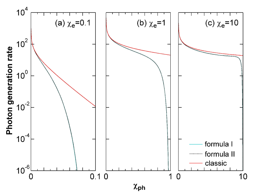
Figure 1: Photon generation rates calculated by formula I [Eq. (1)], formula II [Eq. (4)], and the classic formula [Eq. (5)], respectively. Plots (a), (b), and (c) correspond to different $\chi_{e}$.

We numerically calculate Eqs. (1), (4), and (5), which are denoted by “formula I”, “formula II”, and “classic”, respectively, in Fig. 1. We take a B field with the strength of $b_{0}$ transverse to the electron motion plane. In Fig. 1(a), $b_{0}=200m_{e}c\omega_{0}/e$, $\gamma_{e}=206$ and $\chi_{e}=0.1$; in Fig. 1(b) $b_{0}=2000m_{e}c\omega_{0}/e$, $\gamma_{e}=206$ and $\chi_{e}=1$; and in Fig. 1(c) $b_{0}=2000m_{e}c\omega_{0}/e$, $\gamma_{e}=2060$ and $\chi_{e}=10$. One can see that the formula I and II are nearly the same with different $\chi_{e}$. The classic formula overestimates the rate at the high-energy photon range, as expected. Therefore, one can use either the formula I or the formula II. In the following part and in our simulation we adopt the formula I [Eq. (1)]. Then, we take the pair generation rate Elkina ; Nerush , which have the similar form with Eq. (1). It is given by:

$$\frac{dW_{pair}}{d\xi}=\frac{\alpha m_{e}c^{2}}{\sqrt{3}\pi\hbar\gamma_{ph}}[(\frac{1}{\xi}+\frac{1}{1-\xi}-2)K_{2/3}(\delta)-\int_{\delta}^{\infty}K_{1/3}(s)ds],$$ (6)

where $\delta=2/[3\xi(1-\xi)\chi_{ph}]$, $\xi=\varepsilon_{e}/\varepsilon_{ph}=\gamma_{e}/\gamma_{ph}$, and the energy of the created positron is $\varepsilon_{p}=\varepsilon_{ph}-\varepsilon_{e}$.

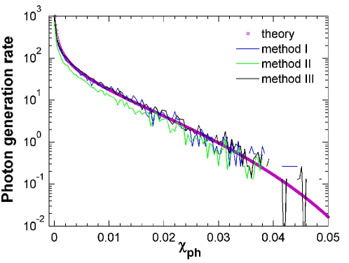
Figure 2: Average rate of photon generation obtained from PIC simulations, where the theoretic values are given by Eq. (1). Three different event generator for photon generation are adopted.

In Figs. 2-4, we benchmark the Monte Carlo simulations by our QED-PIC code against the numerical calculations of Eqs. (1) and (6), respectively. In the simulations, we take $128\times 192$ cells (in $x\times y$) and 1 electron with $\gamma_{e}=206$ per cell. The simulation is run 480 time steps. The obtained average rate of photon generation is shown in Fig. 2. Three methods are respectively adopted for the event generator. Method I: firstly the total generation rate $W_{rad}$ is computed; if $W_{rad}Dt>r_{1}$, a photon will be generated, where $r_{1}$ ($0<r_{1}<1$) is a uniformly-distributed random number; the photon energy with $\varepsilon_{ph}=\xi^{0}\times\varepsilon_{e}$ is obtained through

$$\int_{\xi_{min}}^{\xi^{0}}\frac{dW_{rad}}{d\xi}=r_{2}W_{rad},$$ (7)

where $r_{2}$ ($0<r_{2}<1$) is another uniformly-distributed random number, independent of $r_{1}$. Here, the lower limit of integration $\xi_{min}$ is set to avoid the infrared singularity, where $\xi_{min}\times\varepsilon_{e}=2m_{e}c^{2}$. Method II: firstly a uniformly-distributed random number $r_{3}$ is taken; then a cumulative probability $P_{cum}$ is calculated by $P_{cum}=P_{cum}+W_{rad}Dt$; if $1-\exp(-P_{cum})>r_{3}$, a photon will be generated and the photon has an energy of $\varepsilon_{ph}=\xi^{0}\times\varepsilon_{e}$, where $\xi^{0}$ is obtained through Eq. (7). Method III is similar to the method II, except that the condition of a photon generation is changed to $P_{cum}>r_{3}$. One can see the three methods shows equivalent, as seen in Fig. 2.

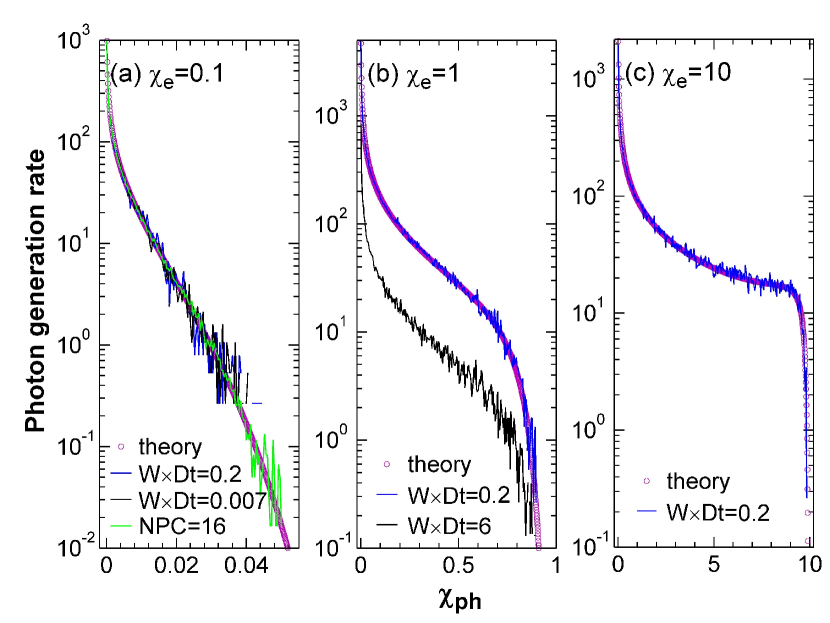
Figure 3: Photon generation rates are obtained from the theory given by Eq. (1), and simulations with different time resolution Dt and different number of particles per cell. In (a)-(c), different $\chi_{e}$ is taken, respectively.

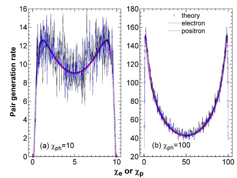
Figure 4: Electron-positron pair generation rates are obtained from the theory given by Eq. (1), and simulations with Dt=$0.2/W$, where different $\chi_{ph}$ is taken in (a) and (b).

In the following simulations, we just take first even generator for both the photons and pairs. Figures 3 and 4 shows the comparison of the photon and pair generation rates given by our PIC simulations against the numerical calculations of Eqs. (1) and (6), respectively. One can see that the two results are in good agreement with different $\chi_{ph}$. We have taken the time step as $Dt=0.2/W$, $W$ is the total rate of photon or pair generation. When the time step is increased to $Dt=6/W$ in Fig. 3(b), the simulation is very different from the theoretical values. When a small enough time step $Dt=0.007/W$ is also taken in Fig. 3(a), the simulation result is nearly the same with the one with $Dt=0.2/W$.

Then, we take an adjustable time step such as when the $W\times Dt>0.2$, the particle generator is automatically separated $N$ steps/circles to meet $W\times Dt/N\leq 0.2$.

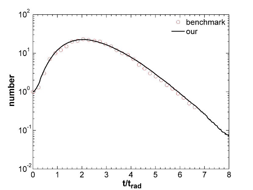
Figure 5: Number of pairs with energy above 100 MeV are created from a cascade. The benchmark data are obtained from the QED-PIC result in Ref. Elkina .

Finally, we benchmark our code against the QED-PIC simulation result Elkina on a cascade development from a single electron with $\gamma=2\times 10^{5}$ initially under a static external magnetic field of $0.2E_{S}$ perpendicularly to the electron motion plane. We counter the created pairs with energy above 100 MeV, as shown in Fig. 5. It is shown that our results agree with the result in Ref. Elkina . Here, $t_{rad}=1.16\times 10^{-16}$ is taken as a characteristic radiation time. Our results are averaged over 4000 simulation runs.

In summary, we have developed our code KLAPS to include QED processes via Monte Carlo methods. This QED-PIC allow us to investigate QED-dominant laser plasma interaction.