Anopheles number prediction on environmental and climate variables using Lasso and stratified two levels cross validation

Abstract

This paper deals with prediction of anopheles number using environmental and climate variables. The variables selection is performed by an automatic machine learning method based on Lasso and stratified two levels cross validation. Selected variables are debiased while the prediction is generated by simple GLM (Generalized linear model). Finally, the results reveal to be qualitatively better, at selection, the prediction, and the CPU time point of view than those obtained by B-GLM method.
Keywords : Malaria, variables selection, Lasso, cross validation, prediction

Introduction

Malaria is endemic in developing countries, mainly in sub-Saharan Africa. Among parasitic diseases , malaria is the main cause of mortality especially for children under five years of age in Africa [1]. Generally, cohort studies take place in endemic areas. some of them are for characterizing the malaria risk (the number of anopheles caught). These cohorts studies are on newborn babies and pregnant women. They are introduced to know about the immunity of newborn face to malaria and the setting of this immunity. They also help to know the determinants implicated in the appearance of first malaria infections on the newborn, the infant exposure to malaria and the malaria risk. It is important to know the interaction between the host and the parasite, the repartition of malaria risk at small scale. This repartition and the malaria risk exposure present simultaneously spatial and temporal dependencies and non-homogeneous at small scale (house level) [2]. Recent studies highlight in the repartition of the malaria risk and transmission, vector profile, ecology, seasonality, characteristics of habitats and the inhabitants practices [2, 3, 4, 5]. It is necessary to understand the relation among the malaria risk and the environmental and climate factors.
In this study, we propose an automatic machine learning method for variables selection combining Lasso, GLM and two levels cross validation in epidemiology context. One of the aim of such approach is to overcome the pre-treatments of experts in medicine and epidemiology on collected data. The proposed approach uses every available explanatory variables without treatment and generates automatically all the interactions among them. This leads to high dimension of variable selection. The Lasso method proposed by Tibshirani [6] is a regularized estimation approach for regression model using an $L_{1}$-norm and constraining the regression coefficients. The results of this method is that all coefficients are shrunken toward zero and some are set exactly to zero. This method simultaneously performs selection and estimation, and it is robust for variables selection in high dimension. In some cohort studies, the number of observations is lower. The classical re-sampling method used is cross validation. It is also well known that cross validation may lead to over fitting and one alternative solution is $percentile-cv$ [7]. To avoid that in learning stage, we propose a stratified cross validation with two levels. According to the nature of the target variable, family of models used for features selection, estimation and prediction are generally linear models, generalized models, mixed models, generalized mixed models, multilevel modeling [2]. The target variable is the number of Anopheles, the main characteristic of malaria risk, it is an account variable. It is well known that the Lasso coefficients are biased. A combination of GLM and Lasso (GLM-Lasso) is performed based on a cross validation with two levels, and a simple GLM is used to debiased Lasso coefficients because of the family of the target variable. For malaria risk prediction, four strategies of variables selection based on GLM-Lasso and cross validation : LDLM, LDLS, FVM, FVS are implemented. These strategies use some criteria : the mean, the quadratic risk, the absolute risk of the predictions, and the deviance of the model. Each strategy is applied on four groups of covariables (original, original with village, recoded, recoded with village). Most of the algorithms implemented in our work are based on [8, 9, 10]. The results are compared to those obtained by reference method (B-GLM) which uses a backward procedure combine with a GLM [2].

The results obtained by such procedure are clearly better improved compared to those obtained by the B-GLM method taken as the reference method. The improvement is about all properties such as the quality of the selection and prediction. Moreover, the CPU time used to display our program is smaller than the one required by the reference method and only few climate and environmental variables are the main factors associated to the malaria risk exposure with an improved accuracy.

Materials and Methods

Materials

In this section, we briefly recall the description of the study area, the mosquito collection and identification as well as the data, and related variables. For more details, see [2].

Study area

The study was conducted in the district of Tori-Bossito (Republic of Benin), from July 2007 to July 2009. Tori-Bossito is on the coastal plain of Southern Benin, 40 kilometers north-east of Cotonou. This area has a subtropical climate and during the study, the rainy season lasted from May to October. Average monthly temperatures varied between 27^∘C and 31^∘C. The original equatorial forest has been cleared and the vegetation is characterized by bushes with sparse trees, a few oil palm plantations, and farms. The study area contained nine villages (Avamé centre, Gbédjougo, Houngo, Anavié, Dohinoko, Gbétaga, Tori Cada Centre, Zébè, and Zoungoudo). Tori Bossito was recently classified as mesoendemic with a clinical malaria incidence of about 1.5 episodes per child per year [11]. Pyrethroid-resistant malaria vectors are present [12].

Mosquito collection and identfication

Entomological surveys based on human landing catches (HLC) were performed in the nine villages every six weeks for two years (July 2007 to July 2009). Mosquitoes were collected at four catch houses in each village over three successive nights (four indoors and four outdoors, i.e. a total of 216 nights every six weeks in the nine villages). Five catch sites had to be changed in the course of the study (2 in Gbedjougo, 1 in Avamè, 1 in Cada, 1 in Dohinoko) and a total of 19 data collections were performed in the field from July 2007 to July 2009. In total, data from 41 catch sites are available. Each collector caught of predictional mosquitoes landing on the lower legs and feet between 10 pm and 6 am. All mosquitoes were held in bags labeled with the time of collection. The following morning, mosquitoes were identified on the basis of morphological criteria [13, 14]. All An. gambiae complex and An. funestus mosquitoes were stored in individual tube with silica gel and preserved at 220^∘C. P. falciparum infection rates were then determined on the head and thorax of individual anopheline specimens by CSP-ELISA [15].

Environnement and behavioral data

Rainfall was recorded twice a day with a pluviometer in each village. In and around each catch site, the following information was systematically collected: (1) type of soil (dry lateritic or humid hydromorphic)—assessed using a soil map of the area (map IGN Benin at 1/200 000 e , sheets NB-31-XIV and NB-31-XV, 1968) that was georeferenced and input into a GIS; (2) presence of areas where building constructions are ongoing with tools or holes representing potential breeding habitats for anopheles; (3) presence of abandoned objects (or ustensils) susceptible to be used as oviposition sites for female mosquitoes; (4) a watercourse nearby; (5) number of windows and doors; (6) type of roof (straw or metal); (7) number of inhabitants; (8) ownership of a bed-net or (9) insect repellent; and (10) normalized difference vegetation index (NDVI) which was estimated for 100 meters around the catch site with a SPOT 5 High Resolution (10 m colors) satellite image (Image Spot5, CNES, 2003, distribution SpotImage S.A) with assessment of the chlorophyll density of each pixel of the image. Due to logistical problems, rainfall measurements are only available after the second entomological survey. Consequently, we excluded the first and second survey (performed in July and August 2007 respectively) from the statistical analyses.

Variables

The dependent variable was the number of Anopheles collected in a house over the three nights of each catch and the explanatory variables were the environmental factors, i.e. the mean rainfall between two catches (classified according to quartile), the number of rainy days in the ten days before the catch (3 classes [0–1], [2–4], $>$4 days), the season during which the catch was carried out (4 classes: end of the dry season from February to April; beginning of the rainy season from May to July; end of the rainy season from August to October; beginning of the dry season from November to January), the type of soil 100 meters around the house (dry or humid), the presence of constructions within 100 meters of the house (yes/no), the presence of abandoned tools within 100 meters of the house (yes/no), the presence of a watercourse within 500 meters of the house (yes/no), NDVI 100 meters around the house (classified according to quartile), the type of roof (straw or Sheet metal), the number of windows (classified according to quartile), the ownership of bed nets (yes/no), the use of insect repellent (yes/no), and the number of inhabitants in the house (classified according to quartile). These pre-treatments based on the knowledge of experts in entomology and medicine operated on some original variables generate a second type of covariables called recoded variables. The Original and recoded variables are described in Tables 3 and 4. Two types of covariables set are used : the first set, the original covariables with all covariables obtained by interactions, the second set, the recoded covariables with all covariables obtained by interactions. For knowing the effect of the village on the selection method and prediction, four groups of covariables are considered : Group 1 (original variables), Group 2 (original variables with village as fixed effect), Group 3 (recoded variables) and Gropu 4 (recoded variables with village as fixed effect)

Interactions between variables

Generally, experts in epidemiology and medicine choose some interactions according to their knowledge and experience. To avoid this way of making, we generate automatically all interactions in the full set of explanatory variables used in the model. This implies that the number of variables exponentially grows and the classical method of variable selection fails. The algorithm developed automatically learns with all variables and all interactions and provides the optimal set of variables for prediction. Assume that $p$ is the number of original covariables, the number of covariables including interactions is $N_{cov}$, $\mathcal{V_{O}}=(V_{1},\ldots,V_{p})$ is a vector of original covariables. The set of interactions covariables is defined as $\mathcal{I}_{\mathcal{V_{O}}}=\{V_{i}:V_{j},1\leq i,j\leq p,\;\;i\neq j\}$, interactions available for : numerical crossed with numerical, numerical crossed with non-numerical and non-numerical crossed with non-numerical covariables. Therefore, the number of covariables of interaction is $p(p-1)/2$ and the total number of variables is $N_{cov}=p+p(p-1)/2$. Assume that the number of observations is $N_{obs}$.

1. Numerical variable crossed with numerical variable :
   $V_{k}$ and $V_{l}$ are two numerical variables. The variable of interaction obtained from $V_{k}$ and $V_{l}$ is noted $V_{k}:V_{l}$ and defined as :

   $$(V_{k}:V_{l})_{i}=(V_{k})_{i}\times(V_{l})_{i},\;1\leq i\leq N_{obs}$$

2. Numerical variable crossed with non-numerical variable :
   $V_{k}$ is a numerical variable and $V_{l}$ a non-numerical variable with $d_{l}$ modalities. $V_{l}$ is considered as a numerical variable with $d_{l}$-dimension. It can be replaced by the indicators of its modalities. Suppose that the modalities are $V_{lq},\;\;1\leq q\leq d_{l}$. The indicator $I_{lq}$ associated to $V_{lq}$ is defined as :

   $$(I_{lq})_{i}=\left\{\begin{array}[]{l}1\;\;\;\mbox{if}\;\;(V_{l})_{i}=V_{lq}\cr 0\;\;\;\mbox{elsewhere}\end{array}\right.$$

   $V_{l}$ can be replaced by $\{I_{lq},\;\;1\leq q\leq d_{l}\}$. The variable of interaction obtained from them is $V_{k}:V_{l}$ with $d_{l}$-dimension and can be replaced by $\{V_{k}:I_{lq},\;\;1\leq q\leq d_{l}\}$. Each $V_{k}:I_{lq}$ is defined as :

   $$(V_{k}:I_{lq})_{i}=\left\{\begin{array}[]{l}(V_{k})_{i}\;\;\;\mbox{if}\;\;(I_{lq})_{i}=1\cr 0\;\;\;\;\;\;\;\;\;\mbox{elsewhere}\end{array}\right.$$

3. Non-numerical variable crossed with non-numerical variable :
   $V_{k}$ and $V_{l}$ are two non-numerical variables with $d_{k}$ and $d_{l}$ modalities respectively. The variable of interaction obtained from $V_{k}$ and $V_{l}$ is $V_{k}:V_{l}$. $V_{k}:V_{l}$ is $d_{k}\times d_{l}$-dimension, can be replaced by $\{I_{kp}:I_{lq},\;\;1\leq p\leq d_{k}\;\;\mbox{and}\;\;1\leq q\leq d_{l}\}$. Each $I_{kp}:I_{lq}$ is defined as :

   $$(I_{kp}:I_{lq})_{i}=\left\{\begin{array}[]{l}1\;\;\;\;\;\;\mbox{if}\;\;(I_{kp})_{i}=(I_{lq})_{i}=1\cr 0\;\;\;\;\;\;\mbox{elsewhere}\end{array}\right.$$

4. Identifiability of variables :
   For the identifiability of variables including those of interactions, a vector $\mathcal{H}$ of integer is automatically generated, $\mathcal{H}=\{h_{1},h_{2},\ldots,h_{N_{cov}}\}$. If $\mathcal{V}$ is the set of all covariables including interactions then $\mathcal{V}=\{V_{1},V_{2},\ldots,V_{N_{cov}}\}$. $\mathcal{H}$ and $\mathcal{V}$ are two vectors with the same length $N_{cov}$. The component $h_{s}$ of $\mathcal{H}$ is the dimension of the covariable $V_{s}$, $1\leq s\leq N_{cov}$. In the process of variables selection, even if a non-numerical variable $V_{s}$ is replaced by the indicators of its modalities, the indicators are automatically identified and grouped according to the component $h_{s}$ of $\mathcal{H}$ corresponding to this covariable.

Methods

The cohort studies generally generate a high data base containing dozens of variables. In the process of analysis of this data, the experts in medicine and epidemiology, use their empirical knowledge on phenomenon to perform pre-treatments which consists in recoding some variables and in choosing some interactions based on expertise. They use classical variables selection methods like wrapper (forward, backward, stepwise, etc.), embedded, filter and ranking to perform variable selection [16]. The goal of wrapper method is to select subset of variables with a lower prediction error. The wrapper algorithm is improved by structural wrapper to obtain a sequence of nested subset of features for optimality [17]. In practice, classical methods of features selection are practically impossible in high dimension because the number of features subsets given by ($2^{p}$), where $p$ is the number of features, increases.
The statistical analysis was conducted in three steps. First, the variables selection is performed using GLM-lasso method through a cross validation with two levels. At the second step, the selected variables are debiased by a GLM and used to predict the number of anopheles. At the last step, the results are compared to those of reference method to clarify which of both methods of variables selection and prediction is better.

Model

The statistical analysis is based on GLM and data are processed using the Lasso method. Such approach is called. GLM-Lasso [18, 19]. The target variable, the number of anopheles conditionally follows a Poisson law. The Poisson laws constitute an exponential family of dispersion and the function density of probability is :

$$\mathcal{P}(y|\mu) = e^{-\mu}\frac{\mu^{y}}{y!}$$ (1)

$$\mathcal{P}(y|\mu) = \frac{1}{y!}\exp\{y\theta-e^{\theta}\}$$ (2)

with $\theta=\log(\mu)$. Its unity variance function is $\mu$ and the deviance associated is defined as :

$$d(y|\mu) = -2\int_{y}^{\mu}\frac{y-u}{u}du$$ (3)

$$d(y|\mu) = -2\left\{(y-y\log(y))-(\mu-y\log(\mu))\right\}$$ (4)

This function is convex, its minimum is null and obtained at $\mu=y$. This implies that $d(y|\mu)$ is positive. The function density of probability can be defined using the deviance as :

$$\mathcal{P}(y|\mu)=\frac{y^{y}e^{-y}}{y!}\exp\left\{-\frac{1}{2}d(y|\mu)\right\}$$ (5)

According to the Equation 5, minimizing the deviance is equivalent to maximizing the likelihood. For each observation $i$, the Equation 5 is defined as:

$$\mathcal{P}(y_{i}|\mu(x_{i},\beta))=\frac{y_{i}^{y_{i}}e^{-y_{i}}}{y_{i}!}\exp\left\{-\frac{1}{2}d(y_{i}|\mu(x_{i},\beta)\right\}$$ (6)

A simple GLM model under matrix shape is :

$$g[E(Y|X,\beta)]=X\beta$$ (7)

where the distribution of $Y$ conditional to $(X=x)$ is the Poisson distribution of parameter $E(Y|X=x,\beta)$, $X$ is the $n\times\,(p+1)$-dimension matrix of covariables (environmental variables), $n$  is the number of observations, $p$ is the number of covariables, $\beta$ is a $(p+1)$-vector of fixed parameters including the intercept, $Y$ is the vector of the target variable.

$$(Y=y_{i}|X=x_{i})\sim\mathbb{P}(\mu_{i});\;\;$$ (8)

where    $x_{i}\beta=\log(\mu_{i})$ and $\mathbb{P}(\mu_{i})$ is a Poisson distribution of parameter $\mu_{i}$. Then

$$\mathbb{P}(Y=y_{i}|X=x_{i})=\frac{e^{(x_{i}\beta)^{y_{i}}}}{(y_{i})!}\times e^{-e^{x_{i}\beta}}$$ (9)

where $y_{i}$ is an integer, $x_{i}$ a vector $(x_{i1},\ldots,x_{ip})$ of real numbers. If $\mathcal{D}=\{(Y=y_{i},X=x_{i}),1\leq i\leq n\}$, the likelihood on $n$ observations can be defined as

$$L_{GLM}(\beta|\;\mathcal{D})=\prod_{i=1}^{n}\frac{e^{(x_{i}\beta)^{y_{i}}}}{(y_{i})!}\times e^{-e^{x_{i}\beta}}$$ (10)

and the log-likelihood is

$$\mathcal{L}_{GLM}(\beta|\;\mathcal{D}) = \log\left(\prod_{i=1}^{n}\frac{e^{(x_{i}\beta)^{y_{i}}}}{(y_{i})!}\times e^{-e^{x_{i}\beta}}\right)$$ (11)

$$\mathcal{L}_{GLM}(\beta|\;\mathcal{D}) = -\sum^{n}_{i=1}\log((y_{i})!)+\sum^{n}_{i=1}y_{i}(x_{i}\beta)-e^{(x_{i}\beta)}$$ (12)

Minimizing the deviance under the constraint $\sum_{i}|\beta_{j}|<t$ which is equivalent to $\lambda\sum_{j}|\beta_{j}|<1$ is reduced to minimizing without constraint on the vector $\beta$ of parameters of the regression function $\sum_{i}d(y_{i}|\mu(x_{i},\beta)+\lambda\sum_{j}|\beta_{j}|$

$$\sum_{i}d(y_{i}|\mu(x_{i},\beta)+\lambda\sum_{j}|\beta_{j}| = -2\sum_{j}(y_{i}-y_{i}\log(y_{i}))-(\mu(x_{i},\beta)-y\log(\mu(x_{i},\beta))$$ (14)

$$+\lambda\sum_{j}|\beta_{j}|$$

$$= +2(\sum_{j}(\mu(x_{i},\beta)-y\log(\mu(x_{i},\beta))+\frac{1}{2}\lambda\sum_{j}|\beta_{j}|)$$ (16)

$$-2\sum_{j}(y_{i}-y_{i}\log(y_{i}))$$

The quantity $\sum_{j}(y_{i}-y_{i}\log(y_{i}))$ does not depend on the parameter $\mu$ of the model then minimizing $\sum_{i}d(y_{i}|\mu(x_{i},\beta)+\lambda\sum_{j}|\beta_{j}|$ is reduced to minimizing $(\sum_{j}(\mu(x_{i},\beta)-y\log(\mu(x_{i},\beta))+\frac{1}{2}\lambda\sum_{j}|\beta_{j}|)$. Using $\lambda$ at the place of $\frac{1}{2}\lambda$, we can minimize $(\sum_{j}(\mu(x_{i},\beta)-y\log(\mu(x_{i},\beta))+\lambda\sum_{j}|\beta_{j}|)$. If

$$Q=\sum_{j}(\mu(x_{i},\beta)-y\log(\mu(x_{i},\beta))+\lambda\sum_{j}|\beta_{j}|$$ (17)

then

$$Q = -\left(\sum_{j}(-\mu(x_{i},\beta)+y\log(\mu(x_{i},\beta))-\lambda\sum_{j}|\beta_{j}|\right)$$ (18)

$$= -\left(\sum_{j}y\log(\mu(x_{i},\beta))-\mu(x_{i},\beta)+\log((y_{i})!)-\lambda\sum_{j}|\beta_{j}|)\right)+\sum_{j}\log((y_{i})!)$$ (19)

$$Q = -(L_{GLM}(\beta|\;\mathcal{D})-\lambda\sum_{j}|\beta_{j}|)+\sum_{j}\log((y_{i})!$$ (21)

Minimizing the quantity Q is the same thing to maximize $L_{GLM}(\beta|\;\mathcal{D})-\lambda\sum_{j}|\beta_{j}|$. Then

$$\mathcal{L}_{pen}(\beta(\lambda)|\;\mathcal{D}) = L_{GLM}(\beta|\;\mathcal{D})-\lambda\sum_{j}|\beta_{j}|$$ (22)

$$\mathcal{L}_{pen}(\beta(\lambda)|\;\mathcal{D}) = -\sum^{n}_{i=1}\log((y_{i})!)+\sum^{n}_{i=1}y_{i}(x_{i}\beta)-e^{(x_{i}\beta)}-\lambda\sum_{j}|\beta_{j}|$$ (23)

According to Equation 22, GLM-Lasso is a regularizing method consisting in penalizing the likelihood of the GLM by adding a penalty term

$$\mathcal{P}(\lambda)=\lambda\sum_{i=1}^{p}{\lvert\beta_{i}\lvert},\;\;\;\mbox{with}\;\;\lambda\geq 0$$ (24)

$$\mathcal{L}_{pen}(\beta(\lambda)|\;\mathcal{D}) = -\sum^{n}_{i=1}\log((y_{i})!)+\sum^{n}_{i=1}y_{i}(x_{i}\beta)-e^{(x_{i}\beta)}-\mathcal{P}(\lambda)$$ (25)

$$\mathcal{L}_{pen}(\beta(\lambda)|\;\mathcal{D}) = L_{GLM}(\beta|\;\mathcal{D})-\mathcal{P}(\lambda)$$ (26)

The coefficients of GLM-Lasso are given by :

$$\hat{\beta}(\lambda)=Arg\max_{\beta}{\left[L_{GLM}(\beta|\;\mathcal{D})-\mathcal{P}(\lambda)\right]}$$ (27)

The choice of the regularizing parameter lambda is done by minimizing a score function. In practice, this equation doesn’t have a good numerical solution. We can use the combination of Laplace approximation, the Newton-Raphson method or Fisher scoring to solve this problem. Such procedure is used at each learning step. The deviance can be defined as :

$$Deviance(\beta|\mathcal{D})=\sum_{i=1}^{n}d(y_{i}|\mu(x_{i},\beta))$$ (28)

where

$$\frac{1}{2}d(y_{i}|\mu(x_{i},\beta)=(y_{i}\log(y_{i})-y_{i})-(y_{i}\log(\mu(x_{i}|\beta))-\mu(x_{i}|\beta))$$ (29)

and $d(y_{i}|\mu(x_{i},\beta)$ is the contribution of the observation $(y_{i},x_{i})$ to the deviance. Then

$$\frac{1}{2}\sum_{i}d(y_{i}|\mu(x_{i},\beta) = \sum_{i}(y_{i}\log(y_{i})-y_{i})-(y_{i}\log(\mu(x_{i}|\beta))-\mu(x_{i}|\beta))$$ (30)

$$= \sum_{i}(y_{i}\log(y_{i})-y_{i}-\log(y_{i}!))$$ (32)

$$-\sum_{i}(y_{i}\log(\mu(x_{i}|\beta))-\mu(x_{i}|\beta)-\log(y_{i}!))$$

$$\frac{1}{2}\sum_{i}d(y_{i}|\mu(x_{i},\beta) = \mathcal{L}(\mathcal{M}{(sat)})-\mathcal{L}(\mathcal{M}{(\beta)})$$ (33)

$$Deviance(\mathcal{M}(\beta)) = 2\left(\mathcal{L}(\mathcal{M}{(sat)})-\mathcal{L}(\mathcal{M}{(\beta)})\right)$$ (34)

where $\mathcal{M}{(sat)}$ is the ”saturated” model and $\mathcal{M}{(\beta)}$ is the model of Poisson regression. It is clear that $Deviance(\mathcal{M}(Sat))=0$.

The deviance of the ’Null’ model noted $\mathcal{M}{(Null)}$ (the model with only the intercept) is defined as :

$$\sum_{i=1}^{n}(y_{i}\log(y_{i})-y_{i})-(y_{i}\log(\bar{y})-\bar{y})$$ (35)

then

$$Deviance(\mathcal{M}(\beta)) = 2\left(\mathcal{L}(\mathcal{M}{(sat)})-\mathcal{L}(\mathcal{M}{(Null)})+\mathcal{L}(\mathcal{M}{(Null)})-\mathcal{L}(\mathcal{M}{(\beta)})\right)$$ (36)

$$Deviance(\mathcal{M}{(\beta)}) = Deviance(\mathcal{M}{(Null)})-2(L(\mathcal{M}{(\beta)})-L(\mathcal{M}{(Null)}))$$ (37)

$$Deviance(\mathcal{M}(\beta)) = Deviance(\mathcal{M}{(Null)})-ResidDev(\mathcal{M}{(\beta)})$$ (38)

$$Deviance(\mathcal{M}{(\beta)}) = Deviance(\mathcal{M}{(Null)})\left(1-\frac{ResidDev(\mathcal{M}{(\beta)})}{Deviance(\mathcal{M}{(Null)})}\right)$$ (39)

Then we have:

$$\frac{Deviance(\mathcal{M}{(\beta)})}{Deviance(\mathcal{M}{(Null)})}=1-\frac{Deviance\;Residual(\mathcal{M}{(\beta)})}{Deviance(\mathcal{M}{(Null)})}$$ (40)

where $ResidDev(\mathcal{M}{(\beta)})=2(L(\mathcal{M}{(\beta)})-L(\mathcal{M}{(Null)}))$ is the residual deviance and $\frac{Deviance(\mathcal{M}{(\beta)})}{Deviance(\mathcal{M}{(Null)})}$ is the ratio of deviances. It is the proportion of the deviance of the Null model explained by the model $\mathcal{M}{(\beta)})$. The residual deviance is positive if

$$\hat{\beta}(\lambda)=Arg\max_{\beta}{\left[L(\mathcal{M}{(\beta)})-\lambda\sum_{j=1}^{p}|\beta_{j}|\right]}$$ (41)

suppose that :

$$R=\frac{Deviance(\mathcal{M}{(\beta)})}{Deviance(\mathcal{M}{(Null)})}\;\mbox{and}\;r=\frac{ResidDev(\mathcal{M}{(\beta)})}{Deviance(\mathcal{M}{(Null)})}$$

The Equation 40 becomes :

$$R=1-r$$ (42)

Minimizing the deviance according to each value of the parameter $\lambda$ of penalty, leads to one model of parameters $\hat{\beta}(\lambda)$ noted $\mathcal{M}{(\hat{\beta}(\lambda))}$.

The aim of GLM-Lasso is to provide a model minimizing the ratio $R$ or maximizing the ratio $r$. Equation 42 gives

$$R=\frac{Deviance(\mathcal{M}{(\hat{\beta}(\lambda_{k}))})}{Deviance((\hat{\beta}(\lambda_{max}))}=1-r$$ (43)

then

$$Deviance(\mathcal{M}{((\hat{\beta}(\lambda_{k}))})=(1-r)\times Deviance(\mathcal{M}{((\hat{\beta}(\lambda_{max}))})$$ (44)

The optimal value $\lambda.min$ of $\lambda$ which minimizes the $Deviance$ function is:

$$\lambda.min=Arg\min_{\lambda_{k}}[Deviance(\mathcal{M}((\hat{\beta}(\lambda_{k})))]$$ (45)

The value $\lambda.1se$ of $\lambda$ defined by T. Hastie et $al$ minimizes the deviance plus its standard deviation [8, 20, 21]:

$$\lambda.1se=Arg\min_{\lambda_{k}}[Deviance(\mathcal{M}(\hat{\beta}(\lambda_{k})))+Std(Deviance(\mathcal{M}(\hat{\beta}(\lambda_{k}))))].$$ (46)

Algorithm (LOLO-DCV)

The algorithm Leave One Level Out Double Cross-Validation (LOLO-DCV) developed in this work is a stratified cross validation with two levels [18, 19]. The second level allows to avoid over-fitting in learning stage in the process of variable selection because the number of observations is lower. Its aim is to compute a second cross validation ($CV_{2}$) for prediction at each step of learning of a first cross validation ($CV_{1}$). The predictors obtained with ($CV_{2}$) are consistent for prediction on the test set for ($CV_{1}$). This algorithm runs as described in Algorithm  1.

Algorithme 1 LOLO-DCV

1. The data are separated in $N_{f}$-folds

2. At each first level $k$

   1. The folds are regrouped in two parts : $A_{k}$ and $E_{k}$, $A_{k}$ : the learning set containing the observations of $(N_{f}-1)$-folds, $E_{k}$ : the test set, containing the observations of the last fold.

   2. Holding-out $E_{k}$

   3. The second level of cross validation

      1. A full cross validation is computed on $A_{k}$

      2. The two regularizing parameters $\lambda.min_{k}$ and $\lambda.1se_{k}$ are obtained.

      3. The coefficients of active variables i.e variables with non-zero coefficients associated to these two parameters are debiased

      4. Predictions are performed using a GLM model on $E_{k}$

      5. The presence $\mathcal{P}(X_{i})$ of each variable is determined using $\lambda.min_{k}$ and $\lambda.1se_{k}$ on $A_{k}$

3. The step  2c is repeated until predictions are performed for all observations.

Quality criteria

The comparison criteria used in this study are :

1. The mean of predictions

2. The quadratic risk of predictions

3. The absolute risk of predictions

4. The deviance of the model

Frequent variables

Let $\mathcal{V}=\{V_{1},V_{2},\ldots,V_{N_{cov}}\}$ be the set of all variables including interactions. According to the algorithm LOLO-DCV 1, at each first level $k,1\leq k\leq N_{f}$, the second level of cross validation provides two values of lambda : $\lambda.min_{k}$ and $\lambda.1se_{k}$ Equation. 45 and 46. $\lambda.min_{k}$ and $\lambda.1se_{k}$ generate two vectors $\beta(\lambda.min_{k})$ and $\beta(\lambda.1se_{k})$ of coefficients of covariables. Based on this, one can determine the presence or the absence of each covariable. For any $\lambda$, let define the function ”Presence” of variable like:

$$\left\{\begin{array}[]{l}\mathcal{P}_{k}(V_{s})=1\;\;\;\mbox{if}\;\;\;\beta_{s}(\lambda)\neq\Theta\cr\mathcal{P}_{k}(V_{s})=0\;\;\;\mbox{elsewhere}\end{array}\right.$$

where $\beta_{s}(\lambda),\;1\leq s\leq N_{cov}$ is a vector of coefficients of covariables $V_{s}$ and $\Theta$ the null vector. The length of $\beta_{s}(\lambda)$ is function of the component $h_{s}$ of $\mathcal{H}$. For a threshold $w,\;\;1\leq w\leq 100$, the set of frequent variables (FV) is

$$\mbox{FV}(\lambda)=\left\{V_{s},\frac{100}{N_{f}}\times\sum_{k=1}^{N_{f}}\mathcal{P}_{k}(V_{s})\geq w\right\}$$ (47)

Variables selection strategies

Four strategies of variables selection are implemented and compared to the reference method. The first strategy, LDLM is based on LOLO-DCV using $\lambda.min$ of Equation. 45. The second strategy, LDLS is based on LOLO-DCV using $\lambda.1se$ of Equation. 46. The third strategy FVM is based on LDLM, and the last FVS is based on LDLS. At the end of the process, LDLM and LDLS select a best subset of covariables and these variables are used to make prediction. The difference between these two strategies is the value of the parameter lambda in Equations. 45 and 46. For the third and the last strategies, at the end of each of the first level of the double cross validation in LDLM and LDLS, the presence of each covariable is computed; at the end of the process, a percentage of presence is evaluated. In these strategies, the minimum $s$ in Equation. 47 is fixed at 100. If the presence percentage is equal or greater than the fixed minimum, this covariable is considered as present and can belong to the subset of frequent variables. The corresponding subset obtained by FVM and FVS is used to predict.

Results

Optimal subset of variables for prediction

In Figure. 1, each vertical band represents a variable and the height of the band is the frequency of the presence of the variable in the strategies FVM and FVS. This figure shows the results in the Group 1. Among 136 variables, FVM selects 13 variables and FVS, 2 variables. The selection in the Group 2 shows that among 153 variables, FVM selects 9 variables and FVS, 2 variables. In the Group 3, based on 136 covariables, FVM selects 11 covariables and FVS, 1 covariable. The selection in the Group 4, shows that among 153 covariables, FVM selects 2 and FVS selects only 1 covariable.
Figure 1. Frequent variables among original variables. At the x-axis, are the variables including interactions and at the y-axis, the percentage of the presence of variables.

Summary of results on prediction accuracy and quality criteria

The Table. 1 contains the results of the reference method B-GLM. The quality of prediction obtained with the subset of variables by FVM and FVS and the predictions of LDLM and LDLS on each Group are described in Table. 2. For these tables, each line represents the results of selection criteria for each strategy.

Table 1: Summary of B-GLM prediction

	Mean	Quadratic risk	Absolute risk	Deviance
B-GLM	3.75	62.29	3.88	3173.9

Table 2: LOLO-DCV on original variables

	Mean	Quadratic risk	Absolute risk	Deviance
LDLM	3.75	72.04	4.48	5573.98
LDLS	3.75	72.04	4.48	5573.98
FVM	3.75	44.35	3.33	3263.03
FVS	3.74	54.54	3.66	3698.18

For the Group 1, Table. 2, FVS has the best mean of prediction, FVM is the best in deviance. The results in the Group 2 shows that FVM has the best mean; it is also the best in deviance. About the Group 3, FVS has the best mean; it is the best in deviance and for the Group 4, FVM has the best mean; it is the best in deviance.

Optimal subset variables of prediction

The best subset of variables selected for each group of covariables is:

1. B-GLM
   According to the results of B-GLM [2], the best subset of covariables is Season (season), the number of rainy days during the three days of one survey (RainyDN), mean rainfall between 2 survey (Rainfall), number of rainy days in the 10 days before the survey (RainyDN102), the use of repellent (Repellent), The index of vegetation (NDVI), the interaction between season and NDVI (season:NDVI).

2. LOLO-DCV (LDLM, LDLS, FVM, and FVS)

   1. Based on the results of Figure. 1 and the Table. 2, the best covariables for the Group 1 (original variables) is Season (season) and interaction between mean rainfall between 2 survey and the number of rainy days during the three days of one survey (Rainfall:RainyDN), results obtained by FVS.

   2. For the Group 2 (original variables with village as fixed effect), the best subset of variables for optimal prediction is Season (season) and interaction between number of rainy days in the 10 days before the survey and village (RainyDN10:village), results obtained by FVS.

   3. The calculations on Group 3 (recoded variables) show that the best subset of covariables is : Season (season) and mean rainfall between 2 survey (RainyDN10), results obtained by FVS.

   4. For the Group 4 (recoded variables with village as fixed effect),

      the best subset of covariables for optimal prediction is: Season (season) and interaction between the number of rainy days during the three days of one survey and presence of work around the site (RainyDN:Works) These results are obtained by FVM.

Discussion

For each group of covariables, the best subset is selected by the trade-off between the application of the criteria and the sparsity of the covariables subset. Globally, the mean in prediction for the four strategies applied on the four groups of covariables is closer to the mean of observations (3.74). LDLM and LDLS achieve exactly the same performance in prediction: mean, quadratic risk, absolute risk and deviance. These two strategies are approximatively the same even if the subset of covariables for the optimal prediction is not the same for the different group of variables. The mean of predictions of both methods are approximatively the same with the mean of observations (3.74) which is achieved exactly by FVS. In prediction, FVM and FVS are better than LDLM and LDLS. The algorithm LOLO-DCV shows the influence of interactions on the target variables. The variability of the score in prediction at village level (high in one the village), detects some problems in the data. The Figure. 1, shows two class of variables, the most frequent and the least frequent. The lowest quadratic risk, absolute risk and deviance are obtained with FVM and FVS. FVS has the same mean in prediction with observations. For Group 1 and Group 2, FVS is the best in prediction but for Group 3 and Group 4, FVM is the best in prediction. The subset of covariables selected by FVS is smaller than the one of FVM for all group of variables. The strategy FVS selects at most 2 variables. It is more sparse than FVM. FVS and FVM achieve the same performance at the absence of village Figures. 1. The presence of village as variable of fixed effect strongly reduces the number of selected variables for optimal prediction. The number of covariables selected in Group 3 and Group 4 is lower than the one of Group 1 and Group 2. The number of covariables with interactions is 136 for Group 1 and Group 3 and 153 for Group 2 and Group 4. The classical methods will compute $2^{136}$ or $2^{153}$ different model before selecting the best subset. Combined with double cross validation, calculation will be unrealizable because of the complexity of the algorithm. The strength of LOLO-DCV is the usage of lasso and the two level cross validation. In a relative short time LOLO-DCV detects all covariables selected by the B-GLM and some interpretable interactions among them. The Tables. 1 and 2, show that LOLO-DCV is the best method in selection and prediction. The distribution of the prediction error according to the classes of anopheles shows a high variability for B-GLM and low for the LOLO-DCV. The optimal subset of features obtained by LOLO-DCV algorithm is approximatively the same at each step. This proves its stability. Finally, the best subset of variables for prediction is composed of variables selected in Group 2, original variables with village as fixed effect, season and interaction between the number of rainy days in the 10 days before the survey and village (RainyDN10 : village) 2b. Its mean in prediction is 3.74.

Conclusion

In this work, we implemented an algorithm for the prediction of malaria risk using environmental and climate variables. We performed the variables selection using an automatic machine learning by a method combining Lasso and stratified two levels cross validation. The selected variables were debiased and the prediction was achieved by simple GLM. The results obtained by such procedure are clearly better improved compared to those obtained by the B-GLM method taken as the reference method. The improvement concerns all properties such as the quality of the selection and prediction. Moreover, the pre-treatments of experts were overcome and the CPU time used to display our program is smaller than the one required by the reference method.

Apendix

Description of original variables

Table 3: Original variables.

	Nature	Number of modalities	Modalities
Repellent	Non-numeric	2	Yes/ No
Bed-net	Non-numeric	2	Yes/ No
Type of roof	Non-numeric	2	Sheet metal/ Straw
Ustensils	Non-numeric	2	Yes/ No
Presence of constructions	Non-numeric	2	Yes/ No
Type of soil	Non-numeric	2	Humid/ Dry
Water course	Non-numeric	2	Yes/ No
Majority Class	Non-numeric	3	1/4/7
Season	Non-numeric	4	1/2/3/4
Village	Non-numeric	9
House	Non-numeric	41
Rainy days before mission	Numeric	Discrete	0/2/$\cdots$/9
Rainy days during mission	Numeric	Discrete	0/1/$\cdots$/3
Fragmentation Index	Numeric	Discrete	26/$\cdots$/71
Openings	Numeric	Discrete	1/$\cdots$/5
Number of inhabitants	Numeric	Discrete	1/$\cdots$/8
Mean rainfall	Numeric	Continue	0/$\cdots$/82
Vegetation	Numeric	Continue	115.2/$\cdots$/ 159.5
Total Mosquitoes	Numeric	Discrete	0/$\cdots$/481
Total Anopheles	Numeric	Discrete	0/$\cdots$/87
Anopheles infected	Numeric	Discrete	0/$\cdots$/9

Description of recoded variables

Table 4: Recoded variables. Variables with star are recoded.

	Nature	Number of modalities	Modalities
Repellent	Non-numeric	2	Yes/ No
Bed-net	Non-numeric	2	Yes/ No
Type of roof	Non-numeric	2	Sheet metal/ Straw
Utensils	Non-numeric	2	Yes/ No
Presence of constructions	Non-numeric	2	Yes/ No
Type of soil	Non-numeric	2	Humid/ Dry
Water course	Non-numeric	2	Yes/ No
Majority class ∗	Non-numeric	3	1/2/3
Season	Non-numeric	4	1/2/3/4
Village∗	Non-numeric	9
House ∗	Non-numeric	41
Rainy days before mission ∗	Non-numeric	3	Quartile
Rainy days during mission	Numeric	Discrete	0/1/$\cdots$/3
Fragmentation index ∗	Non-numeric	4	Quartile
Openings∗	Non-numeric	4	Quartile
Nber of inhabitants ∗	Non-numeric	3	Quartile
Mean rainfall ∗	Non-numeric	4	Quartile
Vegetation∗	Non-numeric	4	Quartile
Total Mosquitoes	Numeric	Discrete	0/$\cdots$/481
Total Anopheles	Numeric	Discrete	0/$\cdots$/87
Anopheles infected	Numeric	Discrete	0/$\cdots$/9

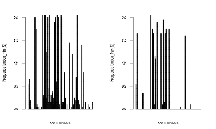
Figure 1: Frequent variables among original variables. At the x-axis, are the variables include interactions and at the y-axis, the percentage of the presence of variables. The sub-figure on left is about $\lambda.min$ and the one on right is about $\lambda.1se.$

References

- [1] WHO (2013) World Health Organisation, World malaria report 2013, World global malaria programme. WHO Library Cataloguing-in-Publication Data : 248.
- [2] Cottrell G, Kouwayè B, Pierrat C, le Port A, Bouraïma A, et al. (2012) Modeling the Influence of Local Environmental Factors on Malaria Transmission in Benin and Its Implications for Cohort Study. PlosOne 7: 8.
- [3] Dery DB, Brown C, Asante KP, Adams M, Dosoo D, et al. (2010) Patterns and seasonality of malaria transmission in the forest-savannah transitional zones of ghana. Malar J 9: 314.
- [4] Craig M, Snow R, Le Sueur D (1999) A climate-based distribution model of malaria transmission in sub-saharan africa. Parasitology today 15: 105–111.
- [5] Gu W, Novak RJ (2005) Habitat-based modeling of impacts of mosquito larval interventions on entomological inoculation rates, incidence, and prevalence of malaria. The American journal of tropical medicine and hygiene 73: 546–552.
- [6] Tibshirani R (1996) Regression shrinkage and selection via the lasso. Journal of the Royal Statistical Society Series B (Methodological) : 267–288.
- [7] Andrew NY (1997) Preventing ”overfitting” of cross-validation data. In: Proceedings of the Fourteenth International Conference on Machine Learning. San Francisco, CA, USA: Morgan Kaufmann Publishers Inc., ICML ’97, pp. 245–253. URL http://dl.acm.org/citation.cfm?id=645526.657119.
- [8] Friedman J, Hastie T, Simon N, Tibshirani R (2015) Lasso and elastic-net regularized generalized linear models. http://www.jstatsoft.org/v33/i01/ R CRAN.
- [9] Goeman JJ (2010) Penalized Estimation in Cox Proportional Hazards Model. Biometrical Journal 52: 70-84.
- [10] Zou H, Hastie T (2005) Regularization and variable selection via the elastic net. Journal of the Royal Statistical Society: Series B (Statistical Methodology) 67: 301–320.
- [11] Damien GB, Djènontin A, Rogier C, Corbel V, Bangana SB, et al. (2010) Malaria infection and disease in an area with pyrethroid-resistant vectors in southern benin. Malaria journal 9: 380.
- [12] Damien GB, Djenontin A, Corbel V, Rogier C, Bangana SB, et al. (2010) Malaria and infection disease in an erea with pyrethroid-resitant vectors in southern Benin. Malaria Journal 9:380.
- [13] Gillies D, Meillon BD (1968) The Anophelinae of Africa south of the Sahara). Pub South Afr Inst Med Res Johannesburg .
- [14] Gillies D, Meillon BD (1987) A supplement to the Anophelinae of Africa south of the Sahara (Afrotropical region). Pub South Afr Inst Med Res .
- [15] Wirtz RA, Zavala F, Charoenvit Y, Campbell GH, Burkot TR, et al. (1987) Comparative testing of monoclonal antibodies against Plasmodium falciparum sporozoites for ELISA development. Bull World Health Organ 65: 39-45.
- [16] Guyon I (2003) An introduction to variable and feature selection. Journal of Machine Learning Research 3: 1157–1182.
- [17] Bontempi G (2005) Structural feature selection for wrapper methods. In: ESANN 2005, 13th European Symposium on Artificial Neural Networks, Bruges, Belgium, April 27-29, 2005, Proceedings. pp. 405–410. URL https://www.elen.ucl.ac.be/Proceedings/esann/esannpdf/es2005-97.pdf.
- [18] Kouwaye B, Fonton N, Rossi F (2015) Sélection de variables par le glm-lasso pour la prédiction du risque palustre. In: 47èmes Journees de Statistique de la SFdS, Lille, France. hal-01196450, Hal.
- [19] Kouwaye B, Fonton N, Rossi F (2015) Lasso based feature selection for malaria risk exposure prediction. In: 11th International Conference, MLDM 2015 Hamburg, Germany, July 2015 Poster Proceedings, ibai publishing. Petra Perner (Ed.), Machine Learning and Data Mining in Pattern Recognition.
- [20] Friedman J, Hastie T, Tibshirani R (2010) Regularization paths for generalized linear models via coordinate descent. Journal of Statistical Software 33: 1–22.
- [21] Hastie TJ, Tibshirani RJ, Friedman JH (2009) The elements of statistical learning : data mining, inference, and prediction. Springer series in statistics. New York: Springer. URL http://opac.inria.fr/record=b1127878. Autres impressions : 2011 (corr.), 2013 (7e corr.).