Three friendly walkers

Abstract

More than 15 years ago Guttmann and Vöge [J. Statist. Plann. Inference, 101, 107 (2002)], introduced a model of friendly walkers. Since then it has remained unsolved. In this paper we provide the exact solution to a closely allied model, originally introduced by Tsuchiya and Katori [J. Phys. Soc. Japan 67, 1655 (1988)], which essentially only differs in the boundary conditions. The exact solution is expressed in terms of the reciprocal of the generating function for vicious walkers which is a D-finite function. However, ratios of D-finite functions are inherently not D-finite and in this case we prove that the friendly walkers generating function is the solution to a non-linear differential equation with polynomial coefficients, it is in other words D-algebraic. We then show via numerically exact calculations that the generating function of the original model can also be expressed as a D-finite function times the reciprocal of the generating function for vicious walkers. We obtain an expression for this D-finite function in terms of a ${}_{2}F_{1}$ hypergeometric function with a rational pullback and its first and second derivatives.

Keywords: Directed walk models, exactly solvable models, D-finite and D-algebraic functions, power-series expansions, asymptotic series analysis

1 Introduction

Consider $p$ directed walkers on the square lattice rotated through $45^{\circ}$ such that each walk take steps in the North-East direction $(1,1)$ or South-East direction $(1,-1)$. The walkers are labelled $k=1,2,\cdots,p$. The positions of the walkers are given by the values of the ordinates $y$ after $t$ steps such that $y^{k}_{t}$ is the ordinate of the $k^{\prime}$th walker after $t$ steps. The walkers are never allowed to cross but they may be allowed to share vertices so $y^{k}_{t}\leq y^{k+1}_{t}$. We consider three versions of the walk problem:

1. Vicious walkers: Walkers are not allowed to share a vertex and hence $y^{k}_{t}<y^{k+1}_{t}$.

2. Friendly walkers: Two walkers may share vertices and edges for any number of steps.

3. Super friendly walkers: Any number of walkers may share vertices and edges for any number of steps.

Figure 1: Examples of a vicious 3-watermelon, a friendly 3-watermelon and a super friendly 3-watermelon. Black edges are singly occupied, red edges are shared by 2 walkers while blue edges are shared by all 3 walkers.

In the most general setting one can study walkers which start at a set of initial points $y^{k}_{0}$ and end at a set of end-points after $n$ steps $y^{k}_{n}$. However, in most cases one places some restrictions on these. Typically one starts the walks at consecutive points such that $y^{k}_{0}=2(k-1)$. With no constraint on the end-points one looks at so-called $p$-stars. If we force the walkers to terminate at consecutive points we are looking at so-called $p$-watermelons. In this paper we study only watermelon configurations. In the super friendly walker case it is perhaps more natural to start all walkers from the origin $y^{k}_{0}=0,\,\forall k$ and also force them to end at the same vertex. Examples of the various models are given in figure 1.

Vicious walkers were introduced into the physics literature by Fisher [1] and the model has been extensively studied since. Despite their simplicity directed walker models have intimate connections to many profound and important physical and mathematical problems. In physics they are often used as simple lattice models of vesicles and polymer networks [1, 2, 3, 4] and deep connections exist to lattice Green functions [5, 6]. The configurations of $p$ vicious walkers can be related to combinatorial objects such as plane partitions [7, 8], Young tableaux [9, 10, 11] and symmetric functions [12]. Exact expressions for the number of configurations of $p$ vicious walkers of length $n$ have been obtained as simple product formulae in particular for the cases of stars and watermelons [4, 9] and in some cases exact closed form expressions have been obtained for the generating functions [4]. Friendly walkers were introduced by Guttmann and Vöge [13] who named them $\infty$-friendly walkers. The super friendly walker model was originally introduced by Tsuchiya and Katori in their studies of directed percolation [14] and a version with interactions used to model polymer fusion or zipping transitions was solved exactly by Tabbara, Owczarek and Rechnitzer [15]. If two walkers are allowed to share a vertex but not an edge one arrives at so-called osculating walkers which can be related to alternating sign matrices [16]. An exact solution for the generating functions of stars and watermelons have been found for $p=3$ [17] and for general $p$ a constant term expression [18] has been proved for the number of osculating configurations of length $n$ with given starting and ending points.

In section 2 we briefly review the results for vicious 3-watermelons and show that the exact generating function obtained by Essam and Guttmann [4] in terms of a Heun function can in fact be expressed in terms of an ${}_{2}F_{1}$ hypergeometric function with a rational pullback and its derivative. In section 3 we prove that the generating functions for a version of friendly 3-watermelons can be expressed in terms of the reciprocal of the generating function of vicious 3-watermelons. We show that the friendly 3-watermelon generating function is not D-finite but is in fact D-algebraic. In section 4 we provide results from a numerical analysis of the singular behaviour of friendly 3-watermelons demonstrating that their generating function have singularities of infinite order. Finally, in section 5 we report on numerically exact computations which show that the generating function of the Guttmann-Vöge model is the ratio of a D-finite function (the solution of a fifth order inhomogenous ODE) and the vicious 3-watermelon generating function. We show that the numerator can be expressed in terms of the ${}_{2}F_{1}$ hypergeometric function appearing in the solution of vicious 3-watermelons and its first and second derivatives.

2 Vicious 3-watermelons

Essam and Guttmann [4, Eq. (63)] proved that the generating function $\mathcal{V}_{3}(x)$ for vicious 3-watermelons is a solution to

$$x^{2}(1+x)(1-8x)G^{\prime\prime}\;+\;x(8-42x-32x^{2})G^{\prime}\;+\;(12-40x-16x^{2})G\;=\;12.$$ (1)

which can be expressed in terms of a Heun function [19]

$$\mathcal{V}_{3}(x) \;=\; \frac{1}{3x^{3}}\left[-1+x-3x^{2}+{\rm HeunG}\left(-\frac{1}{8},-\frac{1}{4};-1,-2,2,-2;-x\right)\right]$$

$$\;=\; \frac{1}{3x^{3}}\left[-1+x-3x^{2}+{\rm HeunG}\left(-8,2;-1,-2,2,-2;8x\right)\right]$$

$$\;=\; 1+2\,x+6\,{x}^{2}+22\,{x}^{3}+92\,{x}^{4}+422\,{x}^{5}+2074\,{x}^{6}+10754\,{x}^{7}+\cdots,$$

where we use the notation adopted in Maple. $\mathcal{V}_{3}(x)$ has singularities at $x=x_{c}=1/8$ and $x=x_{c}=-1$ and at both singularities the critical behaviour is of the form $(1-x/x_{c})^{3}\log(1-x/x_{c})$. Assis et al[20] found that a ${\rm HeunG}$ function with integer coefficients could be recast in terms of an ${}_{2}F_{1}$ hypergeometric function with an algebraic pullback. One of the authors has since told us that generically ${\rm HeunG}$ functions even with rational parameters do not correspond to series with integer coefficients nor can they be recast as series with integer coefficients. Therefore if one sees a ${\rm HeunG}$ function whose series has integer coefficients it probably means that the ${\rm HeunG}$ function is not a generic ${\rm HeunG}$ with four singularities, it is in fact a ${\rm HeunG}$ which can be rewritten as a ${}_{2}F_{1}$ with a pullback that wraps the four singularities of the ${\rm HeunG}$ into the three singularities of the ${}_{2}F_{1}$. So we take a fresh look at the differential operator from (1) giving rise to the ${\rm HeunG}$ solution

$$\qquad L_{\rm H}\;=\;x^{2}(1+x)(1-8x)D_{x}^{2}\;+\;x(8-42x-32x^{2})D_{x}\;+\;(12-40x-16x^{2}).$$ (3)

To check for hypergeometric solutions we turn to the newly developed Maple procedure hypergeometricsols [21, 22] which almost instantaneously finds that the solutions of $L_{\rm H}$ can indeed be expressed in terms of ${}_{2}F_{1}$ hypergeometric functions. The solution corresponding to (2) is

$$\qquad{\rm HeunG}\left(-8,2;-1,-2,2,-2;8x\right)\quad=$$

$$\frac{\left(1-8\,x\right)\left(1+x\right)^{2}}{\left(1-2\,x\right)^{2}}\;{}_{2}F_{1}\left(\left[\frac{1}{3},\frac{2}{3}\right],\,[1],\,{\frac{27\,{x}^{2}}{\left(1-2\,x\right)^{3}}}\right)+$$

$${\frac{x\left(1-8\,x\right)\left(1+x\right)^{2}\left(1+20\,x-8\,{x}^{2}\right)}{\left(1-2\,x\right)^{5}}\;{}_{2}F_{1}\left(\left[\frac{4}{3},\frac{5}{3}\right],\,[2],\,{\frac{27\,{x}^{2}}{\left(1-2\,x\right)^{3}}}\right)}$$ (4)

Now the second ${}_{2}F_{1}$ above is essentially the derivative of the first ${}_{2}F_{1}$. In fact if we let

$$\mathcal{H}(x)\;=\;{}_{2}F_{1}\left(\left[\frac{1}{3},\frac{2}{3}\right],\,[1],\,{\frac{27\,{x}^{2}}{\left(1-2\,x\right)^{3}}}\right)$$ (5)

and

$$\mathcal{R}(x)\;=\;\frac{\left(1-8\,x\right)\left(1+x\right)^{2}}{\left(1-2\,x\right)^{2}}$$ (6)

then

$$\quad{\rm HeunG}\left(-8,2;-1,-2,2,-2;8x\right)=\mathcal{R}(x)\mathcal{H}(x)-\frac{1}{24}(1-8x)(1-2x)^{2}\mathcal{R}^{\prime}(x)\mathcal{H}^{\prime}(x).$$ (7)

We shall see in section 5 that the particular ${}_{2}F_{1}$ hypergeometric function $\mathcal{H}(x)$ appears repeatedly in 3-watermelon problems and hence we shall often make use of the associated differential operator $L_{\mathcal{H}}$ which annihilates $\mathcal{H}(x)$

$$L_{\mathcal{H}} \;=\; x\left(1+x\right)\left(1-8\,x\right)\left(1-2\,x\right)^{2}D_{x}^{2}\;+$$ (8)

$$\left(1-2\,x\right)\left(1-12\,x-24\,{x}^{2}+16\,{x}^{3}\right)D_{x}\;-\;24\,x\left(1+x\right)$$

It may be of some interest to note that the second term in (2) can be re-written (simplified) using Gauss’s contiguous relations so that we get

$$\qquad{\rm HeunG}\left(-8,2;-1,-2,2,-2;8x\right)\quad=$$

$$\frac{\left(1-8\,x\right)\left(1+x\right)^{2}}{\left(1-2\,x\right)^{2}}\;{}_{2}F_{1}\left(\left[\frac{1}{3},\frac{2}{3}\right],\,[1],\,{\frac{27\,{x}^{2}}{\left(1-2\,x\right)^{3}}}\right)+$$

$${\frac{x\left(1+20\,x-8\,{x}^{2}\right)}{\left(1-2\,x\right)^{2}}\;{}_{2}F_{1}\left(\left[\frac{1}{3},\frac{2}{3}\right],\,[2],\,{\frac{27\,{x}^{2}}{\left(1-2\,x\right)^{3}}}\right).}$$ (9)

It is also worth noting that $\mathcal{H}(x)$ can be replaced by the same ${}_{2}F_{1}$ hypergeometric function but with a different rational pullback as a consequence of the identity

$$\quad\frac{1}{1-2x}\cdot{}_{2}F_{1}\left(\left[\frac{1}{3},\frac{2}{3}\right],[1],\frac{27x^{2}}{(1-2x)^{3}}\right)\;=\;\frac{1}{1+4x}\cdot{}_{2}F_{1}\left(\left[\frac{1}{3},\frac{2}{3}\right],[1],\frac{27x}{(1+4x)^{3}}\right)$$ (10)

where the two pullbacks $A(x)=27x^{2}/(1-2x)^{3}$ and $B(x)=27x/(1+4x)^{3}$ are related by a modular curve $\mathcal{C}=0$ with

$$\mathcal{C}\;=\;8A^{3}B^{3}-12A^{2}B^{2}(A+B)+3A\cdot B(2A^{2}+13A\cdot B+2B^{2})-(A+B)(A^{2}+29A\cdot B+B^{2})+27A\cdot B$$

As usual $z=0,1,$ and $\infty$ are singularities of the hypergeometric function ${}_{2}F_{1}([a,b],[c],z)$, and we recall that the hypergeometric differential equation has corresponding exponent pairs $\{0,1-c\}$, $\{0,c-a-b\}$, and $\{a,b\}$, respectively. The condition that the two pullbacks equal 1, yield the singularities $x=1/8$ and $x=-1$. One may think that $x=1/2$ and $x=-1/4$ (such that the pullbacks $A(x)$ and $B(x)$ are $\infty$) are also singularities. This is not the case since $A(-1/4)=1/2$ while $B(1/2)=1/2$, i.e., where one ${}_{2}F_{1}$ appears to be singular the other clearly is not, and one also sees that the singular pre-factors must be cancelled by the ${}_{2}F_{1}$. Likewise, in (2) the singular pre-factors are cancelled when $x=1/2$ which isn’t surprising since obviously $x=1/2$ is not a singularity of $\mathcal{V}_{3}(x)$.

With this in mind one may ask if there is some way of re-writing $\mathcal{H}(x)$ and its companion in (2) so the singular behaviour becomes more transparent. One possibility is to use the Kummer relation

$${}_{2}F_{1}([a,b],[c],z)=(1-z)^{-b}{}_{2}F_{1}([c-a,b],[c],z/(z-1))$$

from which we get

$$\qquad{\rm HeunG}\left(-8,2;-1,-2,2,-2;8x\right)\quad=$$

$$(1-8x)^{1/3}(1+x)^{2/3}{}_{2}F_{1}\left(\left[\frac{2}{3},\frac{2}{3}\right],[1],\frac{-27x^{2}}{(1-8x)(1+x)^{2}}\right)+$$

$${\frac{x\left(1+20\,x-8\,{x}^{2}\right)}{(1-8x)^{2/3}(1+x)^{4/3}}\;{}_{2}F_{1}\left(\left[\frac{2}{3},\frac{5}{3}\right],\,[2],\,\frac{-27x^{2}}{(1-8x)(1+x)^{2}}\right)}$$ (11)

Here at least we can clearly see that $x=1/8$ and $x=-1$ are singular. The integer values of the $c$ parameter means that the singularity at $\infty$ gives rise to an analytic solution and a solution with $\log z$.

3 Vicious and friendly walkers

In this section we consider a variation of friendly 3-watermelons where the walkers start from the origin and end at the same vertex, but other than at the terminals there are never 3 walkers on the same vertex and never do 3 walkers share an edge. We start by proving the following simple result.

Theorem 1.

Vicious and super friendly $p$-watermelons are equinumerous.

Proof.

Let $S_{V}^{n}$ denote the (finite) set of vicious $p$-watermelons and $S_{F}^{n}$ the (finite) set of super friendly $p$-watermelons of length $n$. Let $\phi$ be the function that acting on a vicious $p$-watermelon shifts the $k^{\prime}$th walk downwards by $2(k-1)$ units., i.e, it maps the ordinates of a vicious walker $y^{k}_{t}\to y^{k}_{t}-2(k-1)$ (see figure 2). Since for vicious walkers $y^{k+1}_{t}-y^{k}_{t}\geq 2$ the new configuration is non-crossing and the walkers start at the origin and end at the same point. Hence it is a super friendly $p$-watermelon configuration. This shows that $\phi:S_{V}^{n}\to S_{F}^{n}$ and it is clearly injective. Conversely with the mapping $\phi^{-1}$ we take a friendly $p$-watermelon and shift the $k^{\prime}$th walk upwards by $2(k-1)$ units ($y^{k}_{t}\to y^{k}_{t}+2(k-1)$) resulting in a vicious $p$-watermelon and again this is an injective function. According to the Schröder-Bernstein Theorem we have thus established a bijection between $S_{V}^{n}$ and $S_{F}^{n}$ proving that the two sets have the same cardinality. ∎

Figure 2: The mapping of a vicious 3-watermelon to a super friendly 3-watermelon and back.

We can now proceed to derive an exact expression for the generating function $\mathcal{F}_{3}(x)$ for friendly 3-watermelons.

Theorem 2.

The generating function $\mathcal{F}_{3}(x)$ for friendly 3-watermelons starting from the origin and ending at the same vertex is

$$\mathcal{F}_{3}(x)\;=\;\frac{2(1-x)\mathcal{V}_{3}(x)-1}{\mathcal{V}_{3}(x)}\;=\;2-2x-\frac{1}{\mathcal{V}_{3}(x)}$$

where $\mathcal{V}_{3}(x)$ is the generating function for vicious $3$-watermelons.

Proof.

By Theorem 1 the generating function for super friendly 3-watermelons is $\mathcal{V}_{3}(x)$. Any configuration of super friendly 3-watermelons can be decomposed into a sequence of irreducible components $\omega_{i}$ such that in each component the 3 walkers start at the origin and end on the same vertex but never do the 3 walkers otherwise share the same vertex (see figure 3). Let $G(x)$ denote the generating function for the the set of irreducible components $\omega_{i}$. Since the walkers can take no steps we have

$$\mathcal{V}_{3}(x)=1+G(x)+G(x)^{2}+\cdots=\frac{1}{1-G(x)},$$

which we invert to get

$$G(x) = \frac{\mathcal{V}_{3}(x)-1}{\mathcal{V}_{3}(x)}\;\>=\;\>2\,x+2\,{x}^{2}+6\,{x}^{3}+24\,{x}^{4}+110\,{x}^{5}+550\,{x}^{6}+\cdots.$$

The term $2x$ comes from three walkers simultaneously taking either North-East or South-East steps. These are not permitted friendly configurations so we remove these contributions. The remaining terms all arise from permitted configurations. Then adding in the possibility of taking no steps we finally get

$$\mathcal{F}_{3}(x)\;=\;1-2x+G(x)\;=\;\frac{2(1-x)\mathcal{V}_{3}(x)-1}{\mathcal{V}_{3}(x)}.$$

∎

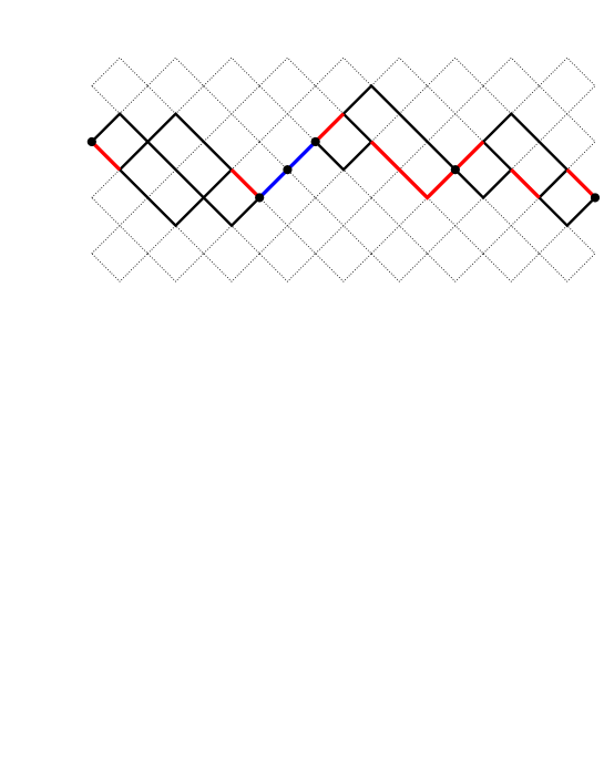
Figure 3: Decomposition of a super friendly 3-watermelon into 5 irreducible components $\omega_{i}$.

We can naturally also express $\mathcal{F}_{3}(x)$ in terms of a Heun function

$$\qquad\mathcal{F}_{3}(x)\;=\;\frac{2-4x+8x^{2}-3x^{3}-2(1-x){\rm HeunG}(-8,2,-1,-2,2,-2,8x)}{1-x+3x^{2}-{\rm HeunG}(-8,2,-1,-2,2,-2,8x)}.$$ (12)

Theorem 2 immediately generalises to friendly $p$-watermelons where up to $p-1$ walkers may share vertices and edges for any number of steps.

Theorem 3.

The generating function $\mathcal{F}_{p}(x)$ for friendly $p$-watermelons starting from the origin and ending at the same vertex with up to $p-1$ walkers allowed to share vertices and edges for any number of steps is

$$\mathcal{F}_{p}(x)\;=\;\frac{2(1-x)\mathcal{V}_{p}(x)-1}{\mathcal{V}_{p}(x)}\;=\;2-2x-\frac{1}{\mathcal{V}_{p}(x)},$$

where $\mathcal{V}_{p}(x)$ is the generating function for vicious $p$-watermelons.

Proof.

Repeat mutatis mutandis the arguments of Theorem 2. ∎

$\mathcal{V}_{3}(x)$ is a D-finite function. So $\mathcal{F}_{3}(x)$ is just a sum of a polynomial and the reciprocal of a D-finite function, but $\mathcal{F}_{3}(x)$ is itself not D-finite. This is not unexpected since generically ratios of D-finite functions are not D-finite, in fact in a quite remarkable paper Harris and Sibuya [23] proved that if both $f$ and $1/f$ are D-finite then $f$ is algebraic. Now clearly given its logarithmic singular behaviour $\mathcal{V}_{3}(x)$ is not algebraic and hence $\mathcal{F}_{3}(x)$ is not D-finite. $\mathcal{F}_{3}(x)$ is however a solution of an algebraic differential equation, i.e., it is D-algebraic. Let $\overline{\mathcal{V}}_{3}(x)=-1/\mathcal{V}_{3}(x)$ then using the Maple package GuessFunc [24] developed by Jay Pantone one quickly finds that $\overline{\mathcal{V}}_{3}(x)$ is a solution to the non-linear D-algebraic equation

$$x^{2}(1+x)(1-8x)\left[R\cdot R^{\prime\prime}-2\left(R^{\prime}\right)^{2}\right]\;+\;2x(4-21x-16x^{2})R\cdot R^{\prime}$$

$$\;-\;\left(12-40x-16{x}^{2}\right)R^{2}\;+\;12\,R^{3}\;=\;0.$$ (13)

This result can be proven by making the substitution $G(x)=-1/R(x)$ in the ODE (1) and expanding. Because of the second derivative there are terms $1/R(x)^{3}$. Hence multiply the resulting equation (after the substitution) by $R(x)^{3}$, collect terms and the result is (3). Then, we find the expression for $\mathcal{F}_{3}(x)=2(1-x)+G(x)$ by substituting $R(x)=G(x)-2(1-x)$ in (3) and evaluating derivatives. We thus prove that

Theorem 4.

The generating function $\mathcal{F}_{3}(x)$ for friendly $3$-watermelons starting from the origin and ending at the same vertex is a solution to the D-algebraic equation

$$x^{2}\left(1+x\right)\left(1-8x\right)F^{\prime\prime}\cdot F\,-\,2\,x^{2}\left(1-x^{2}\right)\left(1-8x\right)F^{\prime\prime}\,-\,2\,x^{2}\left(1+x\right)\left(1-8\,x\right)\left(F^{\prime}\right)^{2}$$

$$+\,2\,x\left(4-21\,x-16\,{x}^{2}\right)F^{\prime}\cdot F\,-\,4\,x\left(4-23\,x-9\,{x}^{2}\right)F^{\prime}\,-\,12\,F^{3}$$ (14)

$$+\,\left(60-32x+16{x}^{2}\right)F^{2}\,-\,\left(96-96x+132{x}^{2}\right)F\,+\,\left(48-64x+176{x}^{2}-48{x}^{3}\right)\;=\;0.$$

4 Singular behaviour of $\mathcal{F}_{3}(x)$

One can easily expand $\mathcal{F}_{3}(x)$ to thousands of terms and perform an asymptotic analysis of the resulting power-series. Using biased differential approximants [25] we find compelling evidence that $\mathcal{F}_{3}(x)$ has a singularity at $x=x_{c}=1/8$ of infinite order with exponents that equal $3k,k\geq 1$, so that the singular behaviour is

$$\sum_{k=1}^{\infty}(1-8x)^{3k}\left[\log(1-8x)\right]^{n_{k}},$$

where possibly $n_{k}=k$. This is exactly the type of behaviour one would expect from the expression (12) where barring some magic cancellations or other simplifications one gets an infinite sum of powers of the ${\rm HeunG}$ function of (2) which has the singular behaviour $(1-8x)^{3}\log(1-8x)$. In table 1 we list as an example the exponent estimates obtained from a single biased differential approximant of order 16 with degrees of polynomials equal to 60 and biasing of order 8 at both $1/8$ and $-1$. These results are quite remarkable in that differential approximants (which essentially approximate a given function by a D-finite one) seems very well-suited to extracting the critical behaviour of $\mathcal{F}_{3}(x)$ which, as we showed above, is in fact not itself D-finite.

Table 1: Biased estimates for the leading critical exponents at the singularities $x_{c}=1/8$ and $x_{c}=-1$ as obtained from a single differential approximant of order 16 and degree 60 for friendly and $\infty$-friendly 3-watermelons.

$\mathcal{F}_{3}(x)$		$\mathcal{F}_{3}^{\infty}(x)$
$\quad x_{c}=1/8$	$\quad x_{c}=-1$	$\quad x_{c}=1/8$	$\quad x_{c}=-1$
$3+1.9\cdot 10^{-127}$	$3+1.8\cdot 10^{-85}$	$3-3.8\cdot 10^{-116}$	$3-4.3\cdot 10^{-56}$
$6-1.3\cdot 10^{-126}$	$4+9.4\cdot 10^{-20}$	$6+2.8\cdot 10^{-92}$	$4-1.8\cdot 10^{-9}$
$9+2.7\cdot 10^{-109}$	$6+1.2\cdot 10^{-66}$	$9+4.2\cdot 10^{-69}$	$6+6.9\cdot 10^{-38}$
$12-5.0\cdot 10^{-83}$	$7-2.0\cdot 10^{-12}$	$12-2.4\cdot 10^{-47}$	$6.99856$
$15+1.4\cdot 10^{-58}$	$9-1.6\cdot 10^{-45}$	$15-6.3\cdot 10^{-28}$	$9-3.8\cdot 10^{-22}$
$18-1.6\cdot 10^{-36}$	$10+3.0\cdot 10^{-4}$	$18+3.8\cdot 10^{-12}$	$12+4.8\cdot 10^{-9}$
$21-4.0\cdot 10^{-17}$	$12-4.9\cdot 10^{-27}$	$21.012$	$15.56563$
$24+9.0\cdot 10^{-5}$	$15-1.9\cdot 10^{-11}$	$58.275$	$-0.75391$

5 Towards a solution for the Guttmann-Vöge model

The model of $\infty$-friendly walkers introduced by Guttmann and Vöge [13] is essentially identical to the model considered above except in boundary conditions. In the $\infty$-friendly walker model the walkers start and finish in a vicious configuration, that is $y^{k}_{0}=2(k-1)$ and if $y^{k}_{t}-y^{k+1}_{t}=2\;(k=1,\cdots,p-1)$ then this is a valid $\infty$-friendly watermelon configuration of length $t$.

The enumeration of these configurations is very fast since one has a polynomial time algorithm. One just keeps track of the ordinates $y^{k}_{t}$. Clearly there is translational invariance in the ordinates so one can always shift the ordinates so $y^{0}_{t}=0$ (alternatively it is the distances between consecutive walkers one needs not their actual positions). So with $p$ walkers and requiring a series to order $n$ one needs on the order of $\left(\!{n/2\atop p-1}\!\right)$ configurations and hence for $p=3$ one has a polynomial time algorithm of complexity $O(n^{2})$. As one moves forward each ordinate can change by $\pm 1$, i.e., $y^{k}_{t+1}=y^{k}_{t}\pm 1$ so that each configuration of ordinates at $t$ produces $2^{p}$ possible new configurations at $t+1$. Any new configuration with $y^{k+1}_{t+1}<y^{k}_{t+1}$ is discarded since this would correspond to walkers crossing. Since only two walkers may share a vertex we also discard configurations if $y^{k+2}_{t+1}=y^{k}_{t+1}$. We start in the ‘vicious’ initial state $y^{k}_{0}=2(k-1)$ and if $y^{k}_{t}-y^{k+1}_{t}=2\;(k=1,\cdots,p-1)$ we add the count of this configuration to the coefficient of $x^{t}$ in the generating function $\mathcal{F}_{p}^{\infty}(x)$.

So one readily calculates long series for the generating function $\mathcal{F}_{3}^{\infty}(x)$ for $\infty$-friendly 3-watermelons. A series analysis shows singularities at $x_{c}=1/8$ and $x_{c}=-1$ and biased differential approximants yields a set of exponents equal to those for $\mathcal{F}_{3}(x)$ (see table 1). So one may hope that $\mathcal{F}_{3}^{\infty}(x)$ is also the ratio of a D-finite function and $\mathcal{V}_{3}(x)$. Hence we form the function $H(x)=\mathcal{F}_{3}^{\infty}(x)\cdot\mathcal{V}_{3}(x)$ and lo and behold amazingly $H(x)$ is indeed D-finite being the solution of an inhomogeneous linear ODE of order 5:

$$\sum_{k=0}^{5}P_{k}(x)\frac{{\rm d}^{k}}{{\rm d}x^{k}}F(x)=P_{\rm I}(x),$$ (15)

where $P_{5}(x)=x^{5}\left(1-8x\right)^{3}\left(1+x\right)^{3}Q_{11}(x)$ with $Q_{11}(x)$ a polynomial of degree 11 whose roots are apparent singularities. The polynomials are listed in A.

The differential operator $L_{5}$ for the homogenous part has a direct sum decomposition into an order two and an order three operator $L_{5}=L_{2}\oplus L_{3}$ as found using the Maple routine DFactorLCLM from the DETools package (the operators are listed in B). The dsolve routine finds that the operator $L_{3}$ has an exact solution in terms of a ${}_{3}F_{2}$ hypergeometric function and two MeijerG functions. It turns out that the MeijerG functions are not relevant solutions so we only list the hypergeometric solution

$$S_{1}(x) \;=\; \frac{\left(1+x\right)^{9}}{x^{9}\left(1-8\,x\right)^{3/2}}\cdot{}_{3}F_{2}\left(\left[\frac{1}{2},\frac{3}{2},\frac{9}{2}\right]\!,\,\left[3,4\right],\,-64\,{\frac{x\left(1+x\right)^{3}}{\left(1-8\,x\right)^{3}}}\right)$$ (16)

dsolve does not find a solution of $L_{2}$. The operator has singularities at $x_{c}=1/8$ and $-1$ with exponents 0 and 3 as did $L_{\rm H}$. So we again turn to hypergeometricsols which immediately finds that the relevant solution of $L_{2}$ can be expressed in terms of $\mathcal{H}(x)$

$$\qquad S_{2}(x)\;=\;\frac{\left(1-8\,x\right)\left(1+x\right)}{{x}^{10}\left(1-2\,x\right)^{2}}\left[x(1+x)P_{1}(x)\mathcal{H}(x)+\frac{1}{12}(1-2\,x)P_{2}(x)\mathcal{H}^{\prime}(x)\right]$$ (17)

with

$$P_{1}(x) \;=\; 137+595\,x-867\,{x}^{2}+1646\,{x}^{3}+298\,{x}^{4}-768\,{x}^{5}$$

$$P_{2}(x) \;=\; 3+87\,x+3701\,{x}^{2}+7198\,{x}^{3}-5956\,{x}^{4}+$$

$$18962\,{x}^{5}-13544\,{x}^{6}+3248\,{x}^{7}-6144\,{x}^{8}$$

The particular solution to the inhomogenous ODE is

$$S_{\rm P}(x)=\frac{1}{9x^{9}}(1+3x-6x^{2}+19x^{3}+6x^{4}+27x^{5}-27x^{6})$$

We then have

$$\mathcal{F}_{3}^{\infty}(x)\cdot\mathcal{V}_{3}(x)\;=\;\frac{1}{9}S_{1}(x)\;-\;\frac{1}{630}S_{2}(x)\;+\;S_{\rm P}(x).$$ (18)

Next we take a closer look at the ${}_{3}F_{2}$ solution to $L_{3}$. We first note that $L_{3}$ has singularities at $x_{c}=1/8$ (and $-1$) with exponents 0, 3 and 12 (9). So there we have that 0 and 3 combination again. This could be a clue that the ${}_{3}F_{2}$ is in fact expressible as a square of $\mathcal{H}(x)$ and its derivatives. To test this we turn to the DETools package. The two routines we need are symmetric power and Homomorphisms. The call symmetric power($L_{\mathcal{H}},2$) calculates a linear differential operator $M$ of minimal order which annihilates any product of solutions of $L_{\mathcal{H}}$, i.e., in particular $\mathcal{H}(x)^{2}$ will be a solution of $M$. Homomorphisms$(M_{1},M_{2})$ calculates (if one exists) a map $R$ (in general this will be a differential operator) such that $R$ maps the solutions of $M_{1}$ to those of $M_{2}$. Concretely this means that if $G(x)$ is a solution of $M_{1}$, i.e., $M_{1}(G)=0$, then $R(G)$ is a solution of $M_{2}$, i.e., $M_{2}(R(G))=0$. The map $R$ is an intertwiner between the two vector spaces of solutions of $M_{1}$ and $M_{2}$. Indeed we find that the call Homomorphisms(symmetric power$(L_{\mathcal{H}},2),L_{3})$ calculates a second order differential operator or intertwiner $I_{3}$, which shows that the solutions of $L_{3}$ can be expressed in terms of the solutions of symmetric power$(L_{\mathcal{H}},2)$. In particular we then get that the relevant solution of $L_{3}$ can be expressed in terms of $\mathcal{H}(x)^{2}$ and derivatives of $\mathcal{H}(x)$. Concretely we can calculate the solution with the call subs($y(x)=\mathcal{H}(x)$, diffop2de($I_{3},y(x))$). We thus find with a bit of straightforward but tedious calculation that

$$6300\,S_{1}(x)=R_{1}(x)\mathcal{H}(x)^{2}+R_{2}(x)\mathcal{H}(x)\mathcal{H}^{\prime}(x)+R_{3}(x)\left(\mathcal{H}(x)\mathcal{H}^{\prime}(x)\right)^{\prime}$$ (19)

where the $R_{k}(x)$ are rational functions listed in C.

So at the end of all this we obtain an expression for $\mathcal{F}_{3}^{\infty}(x)\cdot\mathcal{V}_{3}(x)$ entirely in terms of the simple hypergeometric function

$$\mathcal{H}(x)={}_{2}F_{1}\left(\left[\frac{1}{3},\frac{2}{3}\right],\,[1],\,{\frac{27\,{x}^{2}}{\left(1-2\,x\right)^{3}}}\right)$$

and its first and second derivatives.

6 Conclusion, final remarks and outlook

In this paper we have found the exact solution to a friendly 3-watermelon problem. We proved that the generating function $\mathcal{F}_{3}(x)$ can be expressed as the reciprocal of the vicious 3-watermelon generating function $\mathcal{V}_{3}(x)$ and showed that this result generalise to $p$ walkers. We then showed that the generating function $\mathcal{F}_{3}^{\infty}(x)$ for the Guttmann-Vöge model of infinitely friendly 3-watermelons can be expressed as the ratio of a D-finite function and $\mathcal{V}_{3}(x)$ and we obtained an exact expression for the numerator in terms of a simple ${}_{2}F_{1}$ hypergeometric function and its first and second derivatives.

We also had a look at the Guttmann-Vöge model of 2 friendly walkers [13] in which two walkers may share an edge for a single step after which they have to separate (similar to osculating walkers but on edges rather than vertices). In this case our numerical analysis shows a critical behaviour very similar to that of $\mathcal{F}_{3}(x)$ and $\mathcal{F}_{3}^{\infty}(x)$, but as of yet we have not been able to find an expression for the generating function in terms of $\mathcal{V}_{3}(x)$. We hope to be able to do so in the future.

In future work we plan to study in some detail the friendly $p$-watermelon problem and the problem of $p$-stars as well. We hope that such studies can cast some light on the role of D-algebraic functions in combinatorics and statistical physics.

Jay Pantone has pointed out that it is possible to use the guessed D-finite equation for $H(x)=\mathcal{F}_{3}(x)\mathcal{V}_{3}(x)$ and the known D-finite equation for $\mathcal{V}_{3}(x)$ to recover a conjectured D-algebraic equation for $\mathcal{F}_{3}(x)$ by using the process of differential elimination. The discouraging thing is that the resulting equation is somewhat monstrous. It contains a total of 133 different terms (involving products of powers of $\mathcal{F}_{3}(x)$ and its derivatives) each with a polynomial coefficient of degree up to 51 or so. So it would take between 7000 and 8000 series terms to guess the equation. The highest order derivative occurring in the D-algebraic equation is of order 7 and triple products occur. There are terms such as $\mathcal{F}_{3}^{(5)}\mathcal{F}_{3}^{(7)}$ or $\mathcal{F}_{3}^{(4)}\mathcal{F}_{3}^{(5)}\mathcal{F}_{3}^{(6)}$, where $\mathcal{F}_{3}^{(k)}$ is the $k$’th derivative of $\mathcal{F}_{3}(x)$. Naturally, one would hope that a simpler D-algebraic equation can be found but we have not been successful as yet.

Appendix A The differential operator $L_{5}$

The polynomials $P_{k}(x)\;(k=0,\ldots,5)$ of the differential operator $L_{5}$ and the inhomogenous polynomial $P_{\rm I}(x)$ of (15):

$$P_{5}(x) = x^{5}\left(1-8x\right)^{3}\left(1+x\right)^{3}\Big{(}135+3090\,x-629150\,{x}^{2}+6460390\,{x}^{3}-12243595\,{x}^{4}$$ (20)

$$\;-23887460\,{x}^{5}+80746754\,{x}^{6}-237602788\,{x}^{7}+126388752\,{x}^{8}$$

$$\;-37648256\,{x}^{9}+49950720\,{x}^{10}-3932160\,{x}^{11}\Big{)}$$

$$P_{4}(x) = 5x^{4}\left(1-8x\right)^{2}\left(1+x\right)^{2}\Big{(}1512+25377\,x-6996060\,{x}^{2}+106670412\,{x}^{3}$$

$$-475126952\,{x}^{4}+96806673\,{x}^{5}+2849916588\,{x}^{6}-5502399670\,{x}^{7}$$

$$+9780453960\,{x}^{8}+5163320784\,{x}^{9}-3881744768\,{x}^{10}-715819008\,{x}^{11}$$

$$-2127396864\,{x}^{12}+176160768\,{x}^{13}\Big{)}$$

$$P_{3}(x) = 60x^{3}\left(1-8x\right)\left(1+x\right)\Big{(}2556+26826\,x-11567683\,{x}^{2}+233974966\,{x}^{3}$$

$$-1637367768\,{x}^{4}+3360935670\,{x}^{5}+7477700913\,{x}^{6}-32228461430\,{x}^{7}$$

$$+34977529870\,{x}^{8}-25080039056\,{x}^{9}-116505203984\,{x}^{10}-8874755584\,{x}^{11}$$

$$+28975368704\,{x}^{12}+19194212352\,{x}^{13}+12468813824\,{x}^{14}-1082130432\,{x}^{15}\Big{)}$$

$$P_{2}(x) = 60x^{2}\Big{(}23202+90978\,x-100800276\,{x}^{2}+2549503575\,{x}^{3}-24306318922\,{x}^{4}$$

$$+92736064438\,{x}^{5}-17068101752\,{x}^{6}-721796620433\,{x}^{7}+1283420436692\,{x}^{8}$$

$$-234713753182\,{x}^{9}-1300729277808\,{x}^{10}+5133789454480\,{x}^{11}$$

$$+4644548941696\,{x}^{12}-650017517056\,{x}^{13}-1489831145472\,{x}^{14}$$

$$-997241585664\,{x}^{15}-347227553792\,{x}^{16}+31406948352\,{x}^{17}\Big{)}$$

$$P_{1}(x) = 120x\Big{(}46413+179592\,x-187096284\,{x}^{2}+4466152164\,{x}^{3}-39943265629\,{x}^{4}$$

$$+141983346692\,{x}^{5}-22051491630\,{x}^{6}-971304694080\,{x}^{7}+1699523699010\,{x}^{8}$$

$$-484362312312\,{x}^{9}-1466116591440\,{x}^{10}+5048804828832\,{x}^{11}$$

$$+3936877957248\,{x}^{12}-755770852864\,{x}^{13}-1163160506368\,{x}^{14}$$

$$-758766698496\,{x}^{15}-242406653952\,{x}^{16}+20937965568\,{x}^{17}\Big{)}$$

$$P_{0}(x) = 7698240+22725360\,x-28148670720\,{x}^{2}+634241959920\,{x}^{3}$$

$$-5287126603680\,{x}^{4}+17277689362320\,{x}^{5}-2119806466560\,{x}^{6}$$

$$-100097290614960\,{x}^{7}+170295740442720\,{x}^{8}-54843096571200\,{x}^{9}$$

$$-96884451388800\,{x}^{10}+336731369667840\,{x}^{11}+207092810926080\,{x}^{12}$$

$$-60618583019520\,{x}^{13}-56969296773120\,{x}^{14}-36179450265600\,{x}^{15}$$

$$-10663262945280\,{x}^{16}+869730877440\,{x}^{17}$$

$$P_{\rm I}(x) = 7698240+75796560\,x-27539133120\,{x}^{2}+437080734720\,{x}^{3}$$ (21)

$$-2263546745280\,{x}^{4}+2634702988560\,{x}^{5}+9929567400000\,{x}^{6}$$

$$-19831186297440\,{x}^{7}+17858393541120\,{x}^{8}+2280869253120\,{x}^{9}$$

$$-8302341242880\,x^{10}+1735690813440\,x^{11}+669914234880\,x^{12}.$$

Appendix B The differential operators $L_{3}$ and $L_{2}$ such that $L_{5}=L_{2}\oplus L_{3}$

$$L_{3} \;\;=\;\; x^{3}\left(1+x\right)^{2}\left(1-8\,x\right)^{2}D_{x}^{\,3}\;+$$ (22)

$$x^{2}\left(1+x\right)\left(1-8\,x\right)\left(35-158\,x-112\,{x}^{2}\right)D_{x}^{\,2}\;+$$

$$6\,x\left(62-571\,x+687\,{x}^{2}+1616\,{x}^{3}+512\,{x}^{4}\right)D_{x}\;+$$

$$1188-8460\,x+5712\,{x}^{2}+10752\,{x}^{3}+2304\,{x}^{4}.$$

$$\quad\;\;L_{2} \;=\; x^{2}\left(1+x\right)\left(1-8x\right)Q_{2}(x)D_{x}^{\,2}\;+\;2x\,Q_{1}(x)D_{x}\;+\;Q_{0}(x).$$ (23)

$$Q_{2}(x) \;=\; 4+128\,x+816\,{x}^{2}+3455\,{x}^{3}+3386\,{x}^{4}+10331\,{x}^{5}-$$

$$19058\,{x}^{6}+36333\,{x}^{7}-30148\,{x}^{8}+23970\,{x}^{9}-4608\,{x}^{10},$$

$$Q_{1}(x) \;=\; 42+1014\,x-584\,{x}^{2}-25649\,{x}^{3}-213659\,{x}^{4}-$$

$$288597\,{x}^{5}-825226\,{x}^{6}+625582\,{x}^{7}-883396\,{x}^{8}-$$

$$148802\,{x}^{9}+221034\,{x}^{10}-621888\,{x}^{11}+129024\,{x}^{12},$$

$$Q_{0}(x) \;=\; 396+9216\,x-816\,{x}^{2}-165294\,{x}^{3}-1435806\,{x}^{4}-$$

$$1616220\,{x}^{5}-4745172\,{x}^{6}+3588030\,{x}^{7}-4730706\,{x}^{8}+$$

$$200916\,{x}^{9}+457740\,{x}^{10}-1540800\,{x}^{11}+294912\,{x}^{12}.$$

Appendix C The rational functions of (19)

$$R_{1}(x) = -3\frac{(1-8\,x)(1+x)^{2}\,Q_{1}(x)}{x^{10}(1-2\,x)^{4}}$$

$$Q_{1}(x) = 1-1106\,x+6228\,{x}^{2}+360782\,{x}^{3}+574808\,{x}^{4}$$ (24)

$$750144\,{x}^{5}-909056\,{x}^{6}-444416\,{x}^{7}+24576\,{x}^{8}$$

$$R_{2}(x) = \frac{1}{8}\frac{(1-8\,x)(1+x)\,Q_{2}(x)}{x^{11}(1-2\,x)^{3}}$$

$$Q_{2}(x) = 1+1072\,x-852\,{x}^{2}+345228\,{x}^{3}-3348324\,{x}^{4}-20398920\,{x}^{5}-$$ (25)

$$8922816\,{x}^{6}+40454016\,{x}^{7}+31497216\,{x}^{8}+8126464\,{x}^{9}-$$

$$4653056\,{x}^{10}+393216\,{x}^{11}$$

$$R_{3}(x) = \frac{1}{8}\frac{(1-8\,x)^{2}(1+x)^{2}\,Q_{3}(x)}{x^{10}(1-2\,x)^{2}}$$

$$Q_{3}(x) = 1+904\,x+5544\,{x}^{2}+254312\,{x}^{3}+423416\,{x}^{4}-$$ (26)

$$641856\,{x}^{5}-648704\,{x}^{6}-339968\,{x}^{7}+24576\,{x}^{8}$$

References

References

- [1] Fisher M E 1984 Walks, walls, wetting, and melting J. Stat. Phys. 34 667–729
- [2] Fisher M E, Guttmann A J and Whittington S G 1991 Two-dimensional lattice vesicles and polygons J. Phys. A: Math. Gen. 24 3095–3106
- [3] Brak R, Guttmann A J and Whittington S G 1992 A collapse transition in a directed walk model J. Phys. A: Math. Gen. 25 2437–46
- [4] Essam J W and Guttmann A J 1995 Vicious walkers and directed polymer networks in general dimension Phys. Rev. E 52 5849–5862
- [5] Guttmann A J and Prellberg T 1993 Staircase polygons, elliptic integrals, Heun functions, and lattice Green functions Phys. Rev. E 47 R2233–R2236
- [6] Essam J W 1993 Exact enumeration of parallel walks on directed lattices J. Phys. A: Math. Gen. 26 L863–L869
- [7] Gessel I and Viennot X G 1989 Determinants, paths and plane partitions Preprint
- [8] Stembridge J R 1990 Nonintersecting paths, Pfaffians, and plane partitions Adv. Math. 83 96–131
- [9] Guttmann A J, Owczarek A L and Viennot X G 1998 Vicious walkers and Young tableaux I: Without walls J. Phys. A: Math. Gen. 31 8123–8135
- [10] Krattenthaler C, Guttmann A J and Viennot X G 2000 Vicious walkers, friendly walkers and Young tableaux: II. With a wall J. Phys. A: Math. Gen. 33 8835–8866
- [11] Krattenthaler C, Guttmann A J and Viennot X G 2003 Vicious walkers, friendly walkers, and Young tableaux. III. Between two walls J. Stat. Phys. 110 1069–1086
- [12] Brenti F 1993 Determinants of super-schur functions, lattice paths, and dotted plane partitions Adv. Math. 98 27 – 64
- [13] Guttmann A J and Vöge M 2002 Lattice paths: vicious walkers and friendly walkers J. Statist. Plann. Inference 101 107–131
- [14] Tsuchiya T and Katori M 1998 Chiral Potts models, friendly walkers and directed percolation problem J. Phys. Soc. Japan 67 1655–1666
- [15] Tabbara R, Owczarek A L and Rechnitzer A 2016 An exact solution of three interacting friendly walks in the bulk J. Phys. A: Math. Th. 49 154004
- [16] Brak R 1997 Osculating lattice paths and alternating sign matrices in Proceedings of 9th Formal Power Series and Algebraic Combinatorics Conference (Vienna, Austria)
- [17] Bousquet-Mélou M 2006 Three osculating walkers J. Phys.: Conf. Ser. 42 35–46
- [18] Brak R and Galleas W 2013 Constant term solution for an arbitrary number of osculating lattice paths Lett. Math. Phys. 103 1261–1272
- [19] Ronveaux A, ed. 1995 Heun’s differential equation (Oxford: Oxford University Press)
- [20] Assis M, van Hoeij M and Maillard J M 2016 The perimeter generating functions of three-choice, imperfect, and one-punctured staircase polygons J. Phys. A: Math. Th. 49 214002
- [21] Imamoglu E and van Hoeij M 2015 Maple package hypergeometricsols. Available at http://math.fsu.edu/~eimamogl/hypergeometricsols/
- [22] Imamoglu E and van Hoeij M 2016 Computing hypergeometric solutions of second order linear differential equations using quotients of formal solutions and integral bases Preprint submitted to Journal of Symbolic Computation, arXiv:1606.01576
- [23] Harris W A and Sibuya Y 1985 The reciprocals of solutions of linear ordinary differential equations Adv. Math. 58 119–132
- [24] Pantone J 2016 GuessFunc: Automatically forming conjectures about differentially algebraic power series. In preparation
- [25] Jensen I 2016 Square lattice self-avoiding walks and biased differential approximants Submitted to J. Phys. A. Preprint arXiv: 1607.01109