August, 2016

Non-geometric Five-branes in Heterotic Supergravity

Shin Sasaki and Masaya Yata

Department of Physics
Kitasato University
Sagamihara 252-0373, Japan
Department of Physics,
National University of Singapore
2, Science Drive 3, Singapore 117542, Singapore

We study T-duality chains of five-branes in heterotic supergravity where the first order $\alpha^{\prime}$-corrections are present. By performing the $\alpha^{\prime}$-corrected T-duality transformations of the heterotic NS5-brane solutions, we obtain the KK5-brane and the exotic $5^{2}_{2}$-brane solutions associated with the symmetric, the neutral and the gauge NS5-branes. We find that the Yang-Mills gauge field in these solutions satisfies the self-duality condition in the three- and two-dimensional transverse spaces to the brane world-volumes. The $O(2,2)$ monodromy structures of the $5^{2}_{2}$-brane solutions are investigated by the $\alpha^{\prime}$-corrected generalized metric. Our analysis shows that the symmetric $5^{2}_{2}$-brane solution, which satisfies the standard embedding condition, is a T-fold and it exhibits the non-geometric nature. We also find that the neutral $5^{2}_{2}$-brane solution is a T-fold at least at $\mathcal{O}(\alpha^{\prime})$. On the other hand, the gauge $5^{2}_{2}$-brane solution is not a T-fold but show unusual structures of space-time.

1 Introduction

Extended objects such as branes play an important role in superstring theories. The U-duality [1], which makes non-trivial connections among consistent superstring theories, relates various branes in each theory. It was shown that M-theory compactified on $T^{d}$ has the U-duality symmetry group $E_{d(d)}(\mathbb{R})$ in lower dimensions [2, 3, 4]. BPS branes in superstring theories form lower-dimensional multiplets under the U-duality group. For example, when we consider M-theory compactified on $T^{8}$, we have the $E_{8(8)}(\mathbb{R})$ BPS point particle multiplet. The higher dimensional origin of parts of these point particles is the ordinary branes wrapped/unwrapped on cycles in $T^{8}$. Here, the ordinary branes are waves, F-strings, D-branes, NS5-branes, Kaluza-Klein (KK) branes. However, there are states whose higher dimensional origin does not trace back to the ordinary branes. These states are called exotic states and their higher dimensional origin is known as exotic branes [5, 6].

Among other things, an exotic brane in type II string theories known as the $5^{2}_{2}$-brane, has been studied intensively [7, 8, 9, 10]. The most tractable duality in string theory is the T-duality. Type II string theories compactified on $T^{d}$ has T-duality symmetry group $O(d,d,\mathbb{Z})$. The exotic $5^{2}_{2}$-brane is obtained by performing the T-duality transformations along the transverse directions to the NS5-brane world-volume. As its notation suggests, the $5^{2}_{2}$-brane has two isometries in the transverse directions to the brane world-volume [3]. Its tension is proportional to $g_{s}^{-2}$ where $g_{s}$ is the string coupling constant. Therefore the $5^{2}_{2}$-brane is a solitonic object of co-dimension two. These co-dimension two objects in string theory, sometimes called defect branes [11], exhibit specific properties [12, 13]. When one goes around the center of the co-dimension two branes in the transverse two directions and come back to the original point, the background geometry of the branes changes according to the non-trivial monodromy. Therefore the metric and other background fields are generically governed by multi-valued functions. In this sense, they are called non-geometric [14]. However when the monodromy is given by the symmetry group of the theory, which is generically the U-duality group in string theory, then the non-geometry becomes healthy candidate of solutions to string theory. This kind of solution is called U-fold. An important nature of the exotic branes is that they are non-geometric objects [15]. Therefore they are called non-geometric branes or Q-branes [16]. In particular, the $5^{2}_{2}$-brane in type II string theories is a T-fold, whose monodromy is given by the T-duality group $O(2,2)$.

The purpose of this paper is to study exotic branes in heterotic string theories. Compared with type II string theories, exotic branes in type I and heterotic string theories have been poorly understood. This is due to the non-Abelian gauge field living in the space-time in these theories. Notably, the Yang-Mills gauge field enters into the space-time action as the first order $\alpha^{\prime}$-corrections. Due to the $\alpha^{\prime}$-corrections, the Buscher rule [17] of the T-duality transformation for heterotic supergravity is modified [18, 19, 20]. The most famous extended objects in heterotic supergravity theories are the heterotic NS5-brane solutions. There are three distinct NS5-brane solutions in heterotic supergravity [21, 22, 23]. We will perform the T-duality transformations to these heterotic NS5-branes by the $\alpha^{\prime}$-corrected Buscher rule and obtain new five-brane solutions. We will then study the monodromy structures of these solutions.

The organization of this paper is as follows. In the next section, we introduce the heterotic NS5-brane solutions known as the symmetric, neutral and gauge types [21, 22]. In section 3, we introduce the isometries along the transverse directions to the NS5-brane world-volumes and perform the T-duality transformation by the $\alpha^{\prime}$-corrected Buscher rule. We obtain the heterotic Kaluza-Klein five-brane (KK5-brane) solutions associated with the three types of solutions. We then perform the second T-duality transformations on the KK5-branes and write down the exotic $5^{2}_{2}$-brane solutions. In section 4, we examine the monodromy structure of the heterotic $5^{2}_{2}$-brane solutions by the $\alpha^{\prime}$-corrected generalized metric. We show that the monodromy is given by the $O(2,2)$ T-duality group for the symmetric and the neutral solutions while the gauge solution remains geometric. Section 5 is devoted to conclusion and discussions. The explicit form of the smeared gauge KK5-brane solution is found in appendix.

2 Heterotic NS5-brane solutions

In this section, we introduce the NS5-brane solutions in ten-dimensional heterotic supergravity which is the low-energy effective theory of heterotic superstring theory. Heterotic supergravity consists of the ten-dimensional $\mathcal{N}=1$ gravity multiplet coupled with the $\mathcal{N}=1$ vector multiplet. The relevant bosonic fields in heterotic supergravity are the vielbein $e_{M}{}^{A}$, the dilaton $\phi$, the NS-NS $B$-field $B_{MN}$ and the Yang-Mills gauge field $A_{M}$. Here $M,N,=0,\ldots,9$ are the curved space indices while $A,B,\ldots=0,1,\ldots,9$ are the local Lorentz indices. The Yang-Mills gauge field $A_{M}$ is in the adjoint representation of the gauge group $G$ which is $SO(32)$ or $E_{8}\times E_{8}$. We employ the convention such that the gauge field is represented by anti-hermitian matrices and the trace is taken over the matrices of the fundamental representation.

A remarkable property of heterotic supergravity is that the Yang-Mills gauge field contributes to the action as the first order $\alpha^{\prime}$-correction. The famous anomaly cancellation mechanism and the supersymmetry completion result in the Riemann curvature square term which involves higher derivative corrections in the same order in $\alpha^{\prime}$ [24]. The ten-dimensional heterotic supergravity action for the bosonic fields at the first order in $\alpha^{\prime}$ is given by

$$S= \ \frac{1}{2\kappa^{2}_{10}}\int\!d^{10}x\sqrt{-g}e^{-2\phi}\Bigl{[}R(\omega)-\frac{1}{3}\hat{H}_{MNP}^{(3)}\hat{H}^{(3)MNP}+4\partial_{M}\phi\partial^{M}\phi$$

$$\qquad\qquad\qquad\qquad\qquad\frac{}{}+\alpha^{\prime}\left(\text{Tr}F_{MN}F^{MN}+R_{MNAB}(\omega_{+})R^{MNAB}(\omega_{+})\right)\Bigr{]}.$$ (1)

Here we employ the convention such that $\frac{\kappa^{2}_{10}}{2g^{2}_{10}}=\alpha^{\prime}$ where $\kappa_{10}$ and $g_{10}$ are the gravitational and the gauge coupling constants in ten dimensions. The ten-dimensional metric $g_{MN}$ in the string frame is defined through the vielbein as $g_{MN}=\eta_{AB}e_{M}{}^{A}e_{N}{}^{B}$ where the metric in the local Lorentz frame is $\eta_{AB}=\text{diag}(-1,1,\ldots,1)$. The Ricci scalar $R(\omega)$ is constructed from the spin connection $\omega_{M}{}^{AB}$:

$$R(\omega)= \ e^{M}{}_{A}e^{N}{}_{B}R^{AB}{}_{MN}(\omega),$$

$$R^{AB}{}_{MN}(\omega)= \ \partial_{M}\omega_{N}{}^{AB}-\partial_{N}\omega_{M}{}^{AB}+\omega_{M}{}^{AD}\eta_{CD}\omega_{N}{}^{CB}-\omega_{N}{}^{AD}\eta_{CD}\omega_{M}{}^{CB}.$$ (2)

The spin connection is expressed by the vielbein $e_{M}{}^{A}$ and its inverse:

$$\omega_{M}^{~{}AB}={1\over 2}\Bigl{[}e^{AN}(\partial_{M}e_{N}^{~{}B}-\partial_{N}e_{M}^{~{}B})-e^{BN}(\partial_{M}e_{N}^{~{}A}-\partial_{N}e_{M}^{~{}A})-e^{AP}e^{BQ}(\partial_{P}e_{QC}-\partial_{Q}e_{PC})e_{M}^{~{}C}\Bigr{]}.$$ (3)

The modified spin connection $\omega_{\pm M}{}^{AB}$ which enters into the action in the $\mathcal{O}(\alpha^{\prime})$ terms is defined as

$$\omega_{\pm M}{}^{AB}=\omega_{M}{}^{AB}\pm\hat{H}_{M}^{(3)}{}^{AB},$$ (4)

where $\hat{H}_{M}^{(3)}{}^{AB}=e^{NA}e^{PB}\hat{H}_{MNP}^{(3)}$ and the modified $H$-flux $\hat{H}_{MNP}^{(3)}$ is defined by

$$\hat{H}^{(3)}_{MNP}= \ H_{MNP}^{(3)}+\alpha^{\prime}\left(\Omega_{MNP}^{\text{YM}}-\Omega_{MNP}^{\text{L}+}\right).$$ (5)

Here the field strength $H_{MNP}^{(3)}$ of the $B$-field is defined by

$$H_{MNP}^{(3)}= \ \frac{1}{2}(\partial_{M}B_{NP}+\partial_{N}B_{PM}+\partial_{P}B_{MN}).$$ (6)

The Yang-Mills and the Lorentz Chern-Simons terms which appear in (5) are defined as follows:

$$\Omega^{\text{YM}}_{MNP}= \ 3!\text{Tr}\left(A_{[M}\partial_{N}A_{P]}+\frac{2}{3}A_{[M}A_{N}A_{P]}\right),$$

$$\Omega^{\text{L}+}_{MNP}= \ 3!\left(\eta_{BC}\eta_{AD}\omega_{+[M}{}^{AB}\partial_{N}\omega_{+P]}{}^{CD}+\frac{2}{3}\eta_{AG}\eta_{BC}\eta_{DF}\omega_{+[M}^{AB}\omega_{+N}{}^{CD}\omega_{+P]}{}^{FG}\right).$$ (7)

Here the symbol $[M_{1}M_{2}\cdots M_{n}]$ stands for the anti-symmetrization of indices with weight $\frac{1}{n!}$. Note that the modified $H$-flux is iteratively defined through the relations (4) and (5) order by order in $\alpha^{\prime}$. The modified $H$-flux $\hat{H}^{(3)}$ obeys the following Bianchi identity:

$$d\hat{H}^{(3)}=\alpha^{\prime}\left(\text{Tr}F\wedge F-\text{Tr}R\wedge R\right)+\mathcal{O}(\alpha^{\prime 2}),$$ (8)

where $R^{AB}=\frac{1}{2!}R^{AB}{}_{MN}dx^{M}\wedge dx^{N}$ is the $SO(1,9)$-valued curvature 2-form. The component of the Yang-Mills gauge field strength 2-form $F=\frac{1}{2!}F_{MN}dx^{M}\wedge dx^{N}$ is

$$F_{MN}{}^{I}=\partial_{M}A_{N}^{I}-\partial_{N}A_{M}^{I}+f^{I}{}_{JK}A^{J}{}_{M}A^{K}{}_{N}.$$ (9)

Here $I,J,K=1,\ldots,\text{dim}\mathcal{G}$ are the gauge indices and $f^{I}{}_{JK}$ is the structure constant for the Lie algebra $\mathcal{G}$ associated with $G$. Note that the terms $R_{ABMN}(\omega_{+})R^{ABMN}(\omega_{+})$ and $\Omega^{\text{L}+}_{MNP}$ in the action (1) are higher derivative corrections to the ordinary second order derivative terms.

The heterotic NS5-brane solutions satisfy the equation of motion derived from the action (1) at $\mathcal{O}(\alpha^{\prime})$. There are three distinct NS5-brane solutions known as the symmetric, the neutral and the gauge types in heterotic supergravity [21, 22]. They are 1/2 BPS configurations and preserve a half of the sixteen supercharges. They satisfy the following ansatz:

$$\ ds^{2}=\eta_{ij}dx^{i}dx^{j}+H(r)\delta_{mn}dx^{m}dx^{n},$$

$$\ \hat{H}^{(3)}_{mnp}=-\frac{1}{2}\varepsilon_{mnpq}\partial_{q}H(r),\qquad\phi=\frac{1}{2}\log H(r),$$

$$\ r^{2}=(x^{1})^{2}+(x^{2})^{2}+(x^{3})^{2}+(x^{4})^{2},$$ (10)

where the indices $i,j=0,5,6,7,8,9$, $m,n=1,2,3,4$ represent the world-volume and the transverse directions to the NS5-branes and $\varepsilon_{mnpq}$ is the Levi-Civita symbol. The 1/2 BPS condition leads to the self-duality condition for the Yang-Mills gauge field:

$$F_{mn}=\tilde{F}_{mn},$$ (11)

and other components $A_{i}$ vanish. Here the Hodge dual field strength in the transverse four-dimensions is defined by $\tilde{F}_{mn}=\frac{1}{2}\varepsilon_{mnpq}F^{pq}$. The harmonic function $H(r)$ is determined by the Yang-Mills gauge field configurations of the solutions. These heterotic NS5-branes are characterized by two charges. One is the topological charge $k$ associated with the gauge instantons:

$$k=-\frac{1}{32\pi^{2}}\int\mathrm{Tr}[F\wedge F],$$ (12)

where the integral is defined in the transverse four-space. The other is the charge $Q$ associated with the modified $H$-flux:

$$Q=-\frac{1}{2\pi^{2}\alpha^{\prime}}\int_{S^{3}}\!\hat{H}^{(3)}.$$ (13)

Here $S^{3}$ is the asymptotic three-sphere surrounding the NS5-brane. In the following we briefly introduce the three distinct NS5-brane solutions.

Symmetric solution

The most tractable NS5-brane solution in heterotic theory may be the so-called symmetric solution. The Yang-Mills gauge field which satisfies the self-duality condition (11) is given by an instanton solution in four-dimensions. The gauge field takes value in the $SU(2)$ subgroup of the gauge group $G$ and the explicit solution is given by [22],

$$A_{m}= \ -\frac{\sigma_{mn}x^{n}}{r^{2}+n\alpha^{\prime}e^{-2\phi_{0}}},\quad n\in\mathbb{Z},$$

$$H(r)= \ e^{2\phi_{0}}+\frac{n\alpha^{\prime}}{r^{2}},$$ (14)

where $\sigma_{mn}$ is the self-dual part of the $SO(4)$ Lorentz generator. This is written in the following form,

$$\sigma_{mn}=\eta^{I}_{mn}T^{I},~{}~{}~{}\eta^{I}_{mn}=\varepsilon^{I}_{~{}mn4}+\delta^{I}_{~{}m}\delta_{n4}-\delta^{I}_{~{}n}\delta_{m4},$$ (15)

where $\eta^{I}_{mn}$ is the ’t Hooft symbol which satisfies the self-duality condition in terms of the indices $m,n$:

$$\eta^{I}_{mn}={1\over 2}\varepsilon_{mnpq}\eta^{I}_{pq}.$$ (16)

The anti-hermitian matrices $T^{I}$ are defined as

$$T^{1}=\left[\begin{array}[]{cccc}0&0&0&-1\\ 0&0&1&0\\ 0&-1&0&0\\ 1&0&0&0\end{array}\right],\quad T^{2}=\left[\begin{array}[]{cccc}0&0&-1&0\\ 0&0&0&-1\\ 1&0&0&0\\ 0&1&0&0\end{array}\right],\quad T^{3}=\left[\begin{array}[]{cccc}0&1&0&0\\ -1&0&0&0\\ 0&0&0&-1\\ 0&0&1&0\end{array}\right].$$ (29)

They satisfy the $su(2)$ algebra

$$[T^{I},T^{J}]=-2\varepsilon^{IJK}T^{K},\quad(I,J,K=1,2,3).$$ (30)

The solution (14) is nothing but the BPST one-instanton in the non-singular gauge [25]. The constant $\phi_{0}$ is the asymptotic value of the dilaton. Compared with the general BPST instanton solution, the symmetric solution has a fixed finite instanton size $\rho=e^{-\phi_{0}}\sqrt{n\alpha^{\prime}}$. This solution has charges $(k,Q)=(1,n)$. A remarkable fact about the symmetric solution is that the dilaton configuration, hence the harmonic function $H(r)$, is obtained through the standard embedding ansatz:

$$(A_{m})^{ab}=\omega_{+m}{}^{ab}.$$ (31)

Here the $SU(2)\subset G$ indices $a,b$ of the gauge field are identified with the indices of the $SU(2)$ subgroup of the local Lorentz group $SO(4)$ in the transverse directions. If the relation (31) holds, the Chern-Simons terms in the modified $H$-flux (5) cancel out. Therefore the $H$-flux only comes from the $B$-field and the Bianchi identity (8) becomes $d\hat{H}^{(3)}=0$. From the Bianchi identity and the relation between $H(r)$ and $\hat{H}_{mnp}^{(3)}$ in (10), the $B$-field is determined through the following condition:

$$\partial_{m}H={1\over 2}\varepsilon_{mnpq}\partial_{n}B_{pq}.$$ (32)

Although the symmetric NS5-brane solution (10) with (14) is a solution to the equation of motion derived from the action (1) at $\mathcal{O}(\alpha^{\prime})$, the string sigma-model analysis indicates that the symmetric solution is an exact solution valid at all orders in $\alpha^{\prime}$ [22]. Indeed, the symmetric solution has the $\mathcal{N}=(4,4)$ sigma model description and it is protected against $\alpha^{\prime}$-corrections.

Neutral solution

The neutral solution is the one with charges $(k,Q)=(0,n)$ [22]. For this solution, the Yang-Mills gauge field becomes trivial and the harmonic function is given by

$$A_{M}= \ 0,$$

$$H(r)= \ e^{2\phi_{0}}+\frac{n\alpha^{\prime}}{r^{2}}.$$ (33)

Since the gauge field does not appear in the neutral solution, this is a solution to type II supergravities. Indeed, this is the type II NS5-brane solution. It is remarkable that the neutral solution (10) with (33) for heterotic supergravity is valid at the first order in $\alpha^{\prime}$. For this solution, we find the curvature $R_{MNAB}$ is order $\mathcal{O}(\alpha^{\prime})$. Therefore the Lorentz Chern-Simons term in the modified $H$-flux (5) becomes a higher order correction in $\alpha^{\prime}$ and negligible. Then the Bianchi identity again becomes $d\hat{H}^{(3)}=0$. With the solution (33) at hand, the $B$-field is given by that of the type II NS5-brane and its components, which are determined by (32), are the same as the ones of the symmetric solution in the linear order in $\alpha^{\prime}$. We note that the neutral solution has the $\mathcal{N}=(4,0)$ worldsheet sigma model description and receives higher order $\alpha^{\prime}$-corrections in heterotic theories [22].

Gauge solution

The last is the so called gauge solution which has been originally found in [21]. The Yang-Mills gauge field is again given by the BPST instanton. As in the case of the neutral solution, the curvature term in the modified $H$-flux is neglected as it is a higher order in $\alpha^{\prime}$. However, the Yang-Mills gauge field still contributes to the $H$-flux in the gauge solution and the Bianchi identity becomes $d\hat{H}^{(3)}=\alpha^{\prime}\text{Tr}F\wedge F$. From the Bianchi identity, the harmonic function is determined to be

$$A_{m}= \ -\frac{\sigma_{mn}x^{n}}{r^{2}+\rho^{2}},$$

$$H(r)= \ e^{2\phi_{0}}+8\alpha^{\prime}\frac{r^{2}+2\rho^{2}}{(r^{2}+\rho^{2})^{2}}.$$ (34)

Compared with the symmetric solution (14), the size modulus $\rho$ is not fixed for the gauge solution and it has charges $(k,Q)=(1,8)$. Similar to the neutral solution, the gauge solution is obtained by a perturbative series of $\alpha^{\prime}$ and the functional forms (10), (34) are valid at the first order in $\alpha^{\prime}$. Indeed, the gauge solution has the $\mathcal{N}=(4,0)$ worldsheet sigma model description and is expected to receive higher order $\alpha^{\prime}$-corrections [22]. The position of the instanton corresponds to that of the NS5-brane. Therefore the instanton with finite size $\rho\not=0$ resides in the core of the NS5-brane. It has been discussed in [26], when the instanton shrink to zero size $\rho\to 0$, a gauge multiplet on the brane world-volume becomes massless and the $SU(2)$ gauge symmetry is enhanced. The gauge NS5-brane in the $SO(32)$ heterotic theory in the zero size limit $\rho\to 0$ is related to the D5-brane in type I theory by the S-duality.

We make a comment on the $B$-field for the gauge NS5-brane solution. A careful analysis reveals that only the Yang-Mills Chern-Simons term contributes to the modified $H$-flux and we find $H^{(3)}_{MNP}=0$ at least at $\mathcal{O}(\alpha^{\prime})$. Therefore the $B$-field is not excited in the gauge NS5-brane solution. Then, the components of the $B$-field take a constant value:

$$B_{mn}=\Theta_{mn},~{}~{}~{}(\mbox{constant}).$$ (35)

3 T-duality chains of five-branes and $\alpha^{\prime}$-corrected Buscher rule

In this section, we derive new five-brane solutions in heterotic supergravity in the family of the T-duality chains. Since the gauge field enters into the action (1) as the first order $\alpha^{\prime}$-correction, the T-duality transformation in the heterotic supergravity should be modified from the standard Buscher rule [17]. The first order $\alpha^{\prime}$-corrections to the Buscher rule in heterotic supergravity have been written down in [19]. This is given by

$$g_{\hat{M}\hat{N}}\ \longrightarrow \ g_{\hat{M}\hat{N}}+\frac{1}{G^{\prime}_{yy}}\left(g_{yy}G^{\prime}_{y\hat{M}}G^{\prime}_{y\hat{N}}-G^{\prime}_{yy}g_{y\hat{M}}G^{\prime}_{y\hat{N}}-G^{\prime}_{yy}G^{\prime}_{y\hat{M}}g_{y\hat{N}}\right),$$

$$g_{y\hat{M}}\ \longrightarrow \ -\frac{g_{y\hat{M}}}{G^{\prime}_{yy}}+\frac{g_{yy}G^{\prime}_{y\hat{M}}}{G^{\prime 2}_{yy}},\qquad g_{yy}\ \longrightarrow\ \frac{g_{yy}}{G^{\prime 2}_{yy}},$$

$$B_{\hat{M}\hat{N}}\ \longrightarrow \ B_{\hat{M}\hat{N}}+\frac{1}{G^{\prime}_{yy}}(G^{\prime}_{y\hat{M}}B_{\hat{N}y}-G^{\prime}_{y\hat{N}}B_{\hat{M}y}),\qquad B_{y\hat{M}}\ \longrightarrow\ -\frac{B_{y\hat{M}}}{G^{\prime}_{yy}}-\frac{G^{\prime}_{y\hat{M}}}{G^{\prime}_{yy}},$$

$$\phi\ \longrightarrow \ \phi-\frac{1}{2}\log|G^{\prime}_{yy}|,\qquad A_{\hat{M}}^{I}\ \longrightarrow\ A_{\hat{M}}^{I}-\frac{G^{\prime}_{y\hat{M}}}{G^{\prime}_{yy}}A_{y}^{I},\qquad A_{y}^{I}\ \longrightarrow\ -\frac{A_{y}^{I}}{G^{\prime}_{yy}},$$ (36)

where we have decomposed the indices $M=(\hat{M},y)$. The indices $y$ and $\hat{M},\hat{N}\ldots$ specify an isometry and non-isometry directions respectively. In (36), we have defined the following quantity,

$$G^{\prime}_{MN}=g_{MN}-B_{MN}+2\alpha^{\prime}\bigl{[}\mbox{Tr}(\omega_{+M}\omega_{+N})-\mbox{Tr}(A_{M}A_{N})\bigr{]},$$ (37)

where we have defined $\mbox{Tr}\omega_{+M}\omega_{+N}=\omega_{+M}{}^{AB}\omega_{+NBA}$. We call (36) with (37) the heterotic Buscher rule. Note that when the Yang-Mills gauge field $A_{M}{}^{I}$ and the higher derivative corrections coming from $\omega_{+M}{}^{AB}$ are turned off, the relation (36) reduces to the ordinary Buscher rule for the NS-NS backgrounds in type II supergravities.

3.1 Heterotic KK5-branes

Before going to the exotic $5^{2}_{2}$-branes, we first write down the heterotic KK5-brane solutions. In order to perform the T-duality transformation for the heterotic NS5-brane solutions, we introduce a $U(1)$ isometry along the transverse direction to the brane world-volumes . To this end, we first compactify the $x^{4}$-direction with the radius $R_{4}$ and consider the periodic array of the NS5-branes. Then by taking the small radius limit $R_{4}\to 0$, we introduce the $U(1)$ isometry to the heterotic NS5-brane solutions. The self-duality condition (11) reduces to the monopole equation $\frac{1}{2}\varepsilon_{m^{\prime}n^{\prime}p^{\prime}}F_{n^{\prime}p^{\prime}}=\partial_{m^{\prime}}A_{4}+[A_{m^{\prime}},A_{4}]$ where $m^{\prime},n^{\prime},p^{\prime}=1,2,3$. Therefore the resulting solutions are called the heterotic monopoles or smeared NS5-branes. The explicit forms of the smeared NS5-brane solutions which originate from the periodic arrays of the symmetric, the neutral and the gauge solutions have been written down in [27, 29]. By performing the T-duality transformation of the solutions along the isometry direction, we obtain the KK5-brane solutions associated with the three types of the NS5-branes. In the following, we calculate the T-duality transformations of the NS5-brane solutions and derive the KK5-brane solutions.

Symmetric KK5-brane

For the symmetric solution where the standard embedding condition is satisfied, the ansatz and the Bianchi identity leads to the condition $\Box e^{2\phi}=\Box H=0$. The periodic array of the symmetric NS5-brane solution is governed by the following harmonic function $H(r)$ on $\mathbb{R}^{3}\times S^{1}$ [29]:

$$H(r)=e^{2\phi_{0}}+\sum_{s}\frac{n\alpha^{\prime}}{r^{2}+(x^{4}-2\pi R_{4}s)^{2}},\quad r^{2}=(x^{1})^{2}+(x^{2})^{2}+(x^{3})^{2}.$$ (38)

Taking the compactification radius small $R_{4}\to 0$, the sum in (38) is approximated by the integral over $s$. We call this procedure as smearing. The result is

$$H(r)=e^{2\phi_{0}}+\frac{C}{2r},$$ (39)

The corresponding solution is the smeared symmetric NS5-brane of co-dimension three discussed in [27]. We note that the smeared symmetric NS5-brane is an H-monopole whose quantized charge $Q$ is well-defined. On the other hand, the Yang-Mills monopole charge for the smeared solution is not defined anymore [29]. We now perform the T-duality transformation on the smeared symmetric NS5-brane solution. For a solution where the standard embedding (31) is satisfied, the heterotic Buscher rule (36) is quite simplified. This is because the relation Tr( $\omega_{+M}\omega_{+N})=\mbox{Tr}(A_{M}A_{N})$ holds and the last term in (37) vanishes.

We perform the T-duality transformation by utilizing the heterotic Buscher rule (36). Then we obtain the symmetric KK5-brane solution:

$$ds^{2}= \ \eta_{ij}dx^{i}dx^{j}+H\left[(dx^{1})^{2}+(dx^{2})^{2}+(dx^{3})^{2}\right]+H^{-1}\left[dx^{4}+\beta_{m^{\prime}}dx^{m^{\prime}}\right]^{2},$$

$$\phi= \ 0,\qquad B_{MN}=0,\qquad(m^{\prime}=1,2,3),$$ (40)

where the harmonic function $H$ is given in (39) and $\beta_{m^{\prime}}$ is determined by the following relation:

$$\partial_{m^{\prime}}H=\varepsilon_{m^{\prime}n^{\prime}p^{\prime}}\partial_{n^{\prime}}\beta_{p^{\prime}}.$$ (41)

The dilaton and the NS-NS $B$-field vanish but the Yang-Mills gauge field remains non-trivial. The symmetric KK5-brane solution is not a purely geometric solution but the geometry is dressed up with the Yang-Mills gauge fields. The gauge field $A_{M}{}^{I}$ is obtained as

$$A_{1} ={1\over 2H^{2}}\bigl{[}-\beta_{1}\partial_{1}HT^{1}-(H\partial_{3}H+\beta_{1}\partial_{2}H)T^{2}+(H\partial_{2}H-\beta_{1}\partial_{3}H)T^{3}\bigr{]},$$

$$A_{2} ={1\over 2H^{2}}\bigl{[}(H\partial_{3}H-\beta_{2}\partial_{1}H)T^{1}-\beta_{2}\partial_{2}HT^{2}-(H\partial_{1}H+\beta_{2}\partial_{3}H)T^{3}\bigr{]},$$

$$A_{3} ={1\over 2H^{2}}\bigl{[}-(H\partial_{2}H+\beta_{3}\partial_{1}H)T^{1}+(H\partial_{1}H-\beta_{3}\partial_{2}H)T^{2}-\beta_{3}\partial_{3}HT^{3}\bigr{]},$$

$$A_{4} ={1\over 2H^{2}}\bigl{[}-\partial_{1}HT^{1}-\partial_{2}HT^{2}-\partial_{3}HT^{3}\bigr{]},~{}~{}~{}~{}~{}A_{i}=0.$$ (42)

We find that the Yang-Mills gauge field configuration (42) satisfies the anti-monopole (Bogomol’nyi) equation

$$B_{i}=-D_{i}\phi.$$ (43)

This equation is nothing but the anti-self-duality condition $F_{mn}=-\tilde{F}^{mn}$ in disguise. Since the field configuration (42) satisfies the equation $F_{mn}=-\tilde{F}_{mn}$, this belongs to the general class of spherically symmetric solutions discussed in [28].

Meanwhile, by using the relation (41), the modified spin connection $\omega_{+}$ associated with the geometry (40) is calculated to be

$$\omega_{+1} ={1\over 2H^{2}}\bigl{[}-\beta_{1}\partial_{1}HT^{1}-(H\partial_{3}H+\beta_{1}\partial_{2}H)T^{2}+(H\partial_{2}H-\beta_{1}\partial_{3}H)T^{3}\bigr{]},$$

$$\omega_{+2} ={1\over 2H^{2}}\bigl{[}(H\partial_{3}H-\beta_{2}\partial_{1}H)T^{1}-\beta_{2}\partial_{2}HT^{2}-(H\partial_{1}H+\beta_{2}\partial_{3}H)T^{3}\bigr{]},$$

$$\omega_{+3} ={1\over 2H^{2}}\bigl{[}-(H\partial_{2}H+\beta_{3}\partial_{1}H)T^{1}+(H\partial_{1}H-\beta_{3}\partial_{2}H)T^{2}-\beta_{3}\partial_{3}HT^{3}\bigr{]},$$

$$\omega_{+4} ={1\over 2H^{2}}\bigl{[}-\partial_{1}HT^{1}-\partial_{2}HT^{2}-\partial_{3}HT^{3}\bigr{]},~{}~{}~{}~{}~{}\omega_{+i}=0.$$ (44)

From the results (42) and (44), we find that the standard embedding condition (31) still holds for the symmetric KK5-brane solution.

Neutral KK5-brane

We next study the neutral KK5-brane solution. For the neutral NS5-brane solution, we have the trivial Yang-Mills gauge field $A_{M}{}^{I}=0$. Again, the smearing procedure is applicable to the neutral solution. The smeared neutral NS5-brane solution is governed by the harmonic function (39). As we have claimed in the previous section, the modified spin connection $\omega_{+}$ is in the $\mathcal{O}(\alpha^{\prime})$ for the neutral solution. Therefore it is negligible in $G^{\prime}_{MN}$ in the heterotic Buscher rule (37). Applying the heterotic Buscher rule, we find that the metric, the $B$-field and the dilaton for the neutral KK5-brane solution are given by (40) and the gauge field remains vanishing $A_{M}{}^{I}=0$. Therefore the neutral KK5-brane is a purely geometric Taub-NUT solution at least at the leading order in $\alpha^{\prime}$. Indeed, this is nothing but the KK5-brane solution in type II theories.

Gauge KK5-brane

For the gauge NS5-brane solution, the periodic harmonic function (39) does not work as a solution since $\Box e^{2\phi}=0$ is not satisfied for the gauge solution. The ansatz (10) and the Bianchi identity indicates $\Box H(r)=\frac{\alpha^{\prime}}{2}\mathrm{Tr}[\varepsilon^{mnpq}F_{mn}F_{pq}]$. In order to find a solution of co-dimension three associated with the gauge solution, we perform the singular gauge transformation of the solution (34). Then the gauge field becomes

$$A_{m}=\frac{-2\rho^{2}\bar{\sigma}_{mn}x^{n}}{r^{2}(r^{2}+\rho^{2})},\qquad r^{2}=(x^{1})^{2}+(x^{2})^{2}+(x^{3})^{2}+(x^{4})^{2},$$ (45)

where $\bar{\sigma}_{mn}$ is the antisymmetric and anti-self-dual matrix and is written as

$$\bar{\sigma}_{mn}=\overline{\eta}^{I}_{mn}T^{I},~{}~{}~{}\bar{\eta}^{I}_{mn}=\varepsilon^{I}_{~{}mn4}-\delta^{I}_{~{}m}\delta_{n4}+\delta^{I}_{~{}n}\delta_{m4}.$$ (46)

This is the BPST instanton in the singular gauge. The solution is obtained by the famous ’t Hooft ansatz:

$$A_{m}=\bar{\sigma}_{mn}\partial_{n}\log f.$$ (47)

The function $f$ satisfies $\frac{1}{f}\Box f=0$ and given by $f(r)=1+\sum_{i=1}^{k}\frac{\rho^{2}}{(x-x_{i})^{2}}$ for the $k$-instanton solution. Here $x_{i}$ are the positions of the instantons. Note that the solution (45) corresponds to $k=1$. Using this fact, we can perform the smearing procedure for $f$ along the line of obtaining (39). This periodic array of the instantons is just the calorons of the Harrington-Shepard type [30]. The harmonic function $H$ for the smeared gauge NS5-brane is determined by the Laplace equation whose source is given by the $R_{4}\to 0$ limit of the calorons, namely, the smeared instantons. After the smearing, we find $f=1+\frac{\tilde{\rho}}{r}$ where $r^{2}=(x^{1})^{2}+(x^{2})^{2}+(x^{3})^{2}$ and $\tilde{\rho}=\frac{\rho^{2}}{2R_{4}}$ is a rescaled size modulus. Then the smeared gauge NS5-brane solution is found to be

$$ds^{2} =\eta_{ij}dx^{i}dx^{j}+e^{2\phi}\delta_{mn}dx^{m}dx^{n},$$

$$A_{m} =\bar{\sigma}_{mn}{-\tilde{\rho}x^{\nu}\over r^{2}(r+\tilde{\rho})},~{}~{}~{}~{}~{}e^{2\phi}=e^{2\phi_{0}}-2\alpha^{\prime}{\tilde{\rho}^{2}\over r^{2}(r+\tilde{\rho})^{2}},~{}~{}~{}~{}~{}\hat{H}_{mnp}^{(3)}=-{1\over 2}\varepsilon_{mnpq}\partial_{q}e^{2\phi}.$$ (48)

As in the case of the gauge NS5-brane solution, we find that the $B$-fields in the smeared gauge NS5-brane solution becomes trivial. This property is also found in the heterotic monopole solution [29]. We also note that the smeared gauge NS5-brane does not exhibit the H-monopole property. Indeed, we find the modified $H$-flux behaves like $\hat{H}^{(3)}_{mn4}\sim 4\alpha^{\prime}\tilde{\rho}\epsilon_{mnq4}\frac{x^{q}}{r^{6}}\ (r\to\infty)$ and the charge $Q$ vanishes. This is in contrast to the symmetric and the neutral solutions. We also comment that the solution (48) based on the smeared instanton does not have a finite monopole charge. This is again in contrast to the monopole solution in [29].

Since the $B$-field is trivial in the gauge solution, we can set these components as

$$B_{14}=\Theta_{1},~{}~{}~{}B_{24}=\Theta_{2},~{}~{}~{}B_{34}=\Theta_{3},$$ (49)

where $\Theta_{i}$ are constants. The other components do not appear in the solution and they can be set to zero. Now we perform the T-duality transformation of the smeared gauge NS5-brane solution along the $x^{4}$-direction. After calculations, we find the following gauge KK5-brane solution:

$$ds^{2} =\eta_{ij}dx^{i}dx^{j}+{\cal H}\delta_{m^{\prime}n^{\prime}}dx^{m^{\prime}}dx^{n^{\prime}}+e^{-4\phi_{0}}{\cal H}(dx^{4}+\Theta_{m^{\prime}}dx^{m^{\prime}})^{2},$$

$$\phi ={1\over 2}\log e^{-4\phi_{0}}{\cal H},~{}~{}~{}~{}~{}{\cal H}=e^{2\phi_{0}}-2\alpha^{\prime}{\tilde{\rho}^{2}\over r^{2}(r+\tilde{\rho})^{2}},$$

$$A_{1} ={\tilde{\rho}\over 2r^{2}(r+\tilde{\rho})}\Bigl{(}(x^{3}T^{2}-x^{2}T^{3})+e^{-2\phi_{0}}\Theta_{1}(x^{1}T^{1}+x^{2}T^{2}+x^{3}T^{3})\Bigr{)},$$

$$A_{2} ={\tilde{\rho}\over 2r^{2}(r+\tilde{\rho})}\Bigl{(}(x^{1}T^{3}-x^{3}T^{1})+e^{-2\phi_{0}}\Theta_{2}(x^{1}T^{1}+x^{2}T^{2}+x^{3}T^{3})\Bigr{)},$$

$$A_{3} ={\tilde{\rho}\over 2r^{2}(r+\tilde{\rho})}\Bigl{(}(x^{2}T^{1}-x^{1}T^{2})+e^{-2\phi_{0}}\Theta_{3}(x^{1}T^{1}+x^{2}T^{2}+x^{3}T^{3})\Bigr{)},$$

$$A_{4} =e^{-2\phi_{0}}{\rho^{2}\over 2r^{2}(\rho^{2}+r)}(x^{1}T^{1}+x^{2}T^{2}+x^{3}T^{3}),\quad A_{i}=0.$$ (50)

The solution seems complicated but one finds that the Yang-Mills gauge field satisfies the anti-monopole equation (43). Notably, the function $\mathcal{H}$ becomes negative at a finite value of $r$. The solution is ill-defined near the center of the brane. This property is similar to the symmetric and neutral NS5-brane solutions with $n<0$ whose physical interpretation is unclear [29].

3.2 Heterotic $5^{2}_{2}$-branes

Now we are in a position where the second T-duality transformation is performed on the KK5-brane solutions. We introduce another isometry along the transverse direction $x^{3}$ to the KK5-brane world-volumes. By performing the second T-duality transformation along the $x^{3}$-direction, we obtain the exotic $5^{2}_{2}$-brane solutions associated with the symmetric, the neutral and the gauge solutions.

Symmetric $5^{2}_{2}$-brane

The harmonic function $H(r)$ in $\mathbb{R}^{2}\times T^{2}$ is obtained by the periodic array of the KK5-brane. This is given by

$$H(r)= \ e^{2\phi_{0}}+\frac{1}{2}\sum_{s}\frac{n\alpha^{\prime}R_{3}^{-1}}{\sqrt{r^{2}+(x^{3}-2\pi R_{3}s)^{2}}},$$

$$r^{2}= \ (x^{1})^{2}+(x^{2})^{2}.$$ (51)

Taking the compactification radius small $R_{3}\to 0$, the sum in (51) is approximated by the integral over $s$ with the cutoff scale $\Lambda$. The result is [15]

$$H(r)=h_{0}-\frac{\sigma}{2}\log\frac{r}{\mu},$$ (52)

where $\sigma=\frac{R_{3}R_{4}}{2\pi\alpha^{\prime}}$ and $\mu$ is a constant which specifies the region where the solution is valid [31]. The constant $h_{0}$ diverges in the large cutoff scale limit $\Lambda\to\infty$. Since the harmonic function only depends on $x^{1},x^{2}$, the NS-NS $B$-field does so. The only non-zero component of the $B$-field $B_{34}=\omega$ is determined by the following relations:

$$\partial_{1}H=\partial_{2}\omega,\qquad\partial_{2}H=-\partial_{1}\omega,$$ (53)

The explicit form of $\omega$ is found to be

$$\omega=-\sigma\tan^{-1}\left(\frac{x^{2}}{x^{1}}\right).$$ (54)

If we employ the coordinate system $x^{1}=r\cos\theta,x^{2}=r\sin\theta$ where $\theta$ is the angular coordinate in the $x^{1}x^{2}$-plane, then $\omega$ is proportional to $\theta$. This result leads to the fact that the space-time metric, the dilaton and the NS-NS $B$-field in the solution are not single-valued anymore. The logarithmic behaviour of the harmonic function is characteristic to co-dimension two objects. We call the solution (40) on which the harmonic function is replaced by (52) the smeared symmetric KK5-brane solution. Indeed, the heterotic vortex and the domain wall are discussed in [32, 33] where the harmonic function behaves as logarithmic and linear functions.

Since the heterotic KK5-brane solution satisfies the standard embedding condition, this again simplify the heterotic Buscher rule (36). By performing the second T-duality transformation along the $x^{3}$-direction, we obtain the following symmetric $5^{2}_{2}$-brane solution:

$$ds^{2}= \ \eta_{ij}dx^{i}dx^{j}+H\left[(dx^{1})^{2}+(dx^{2})^{2}\right]+\frac{H}{K}\left[(dx^{3})^{2}+(dx^{4})^{2}\right],$$

$$\phi= \ \frac{1}{2}\log\frac{H}{K},\quad B_{34}=-\frac{\omega}{K},\quad K=H^{2}+\omega^{2}.$$ (55)

The metric, the dilaton and the NS-NS $B$-field in (55) are the same with the ones in type II theory. However, in heterotic theory, the Yang-Mills gauge field remains non-trivial. The gauge field $A_{M}{}^{I}$ is calculated as

$$A_{1} ={1\over 2H}(\partial_{2}H)T^{3},~{}~{}~{}~{}~{}A_{2}=-{1\over 2H}(\partial_{1}H)T^{3},$$

$$A_{3} ={1\over 2HK}\Bigl{(}(H\partial_{2}H+\omega\partial_{1}H)T^{1}-(H\partial_{1}H-\omega\partial_{2}H)T^{2}\Bigr{)},$$

$$A_{4} =-{1\over 2HK}\Bigl{(}(H\partial_{1}H-\omega\partial_{2}H)T^{1}+(H\partial_{2}H+\omega\partial_{1}H)T^{2}\Bigr{)},$$

$$A_{i} =0.$$ (56)

We find that (56) satisfies the vortex-like equation in two dimensions:

$$D_{1}\varphi-iD_{2}\varphi=0,\qquad[\varphi,\bar{\varphi}]=B_{3},$$ (57)

where $\varphi=\frac{1}{\sqrt{2}}(A_{3}+iA_{4})$ is a complexified adjoint scalar field. The vortex-like equation (57) is obtained by dimensionally reducing the self-duality condition (11) to two dimensions. We note that since the Yang-Mills gauge field contains the explicit angular coordinate in $\omega$, $A_{m}$ is not a single-valued function also in the symmetric $5^{2}_{2}$-brane solution.

The modified spin connection $\omega_{+}$ associated with the solution (55) is calculated as

$$\omega_{+1}=\frac{1}{2H}(\partial_{2}H)T^{3}+K^{-1}\left(H\partial_{2}H+\omega\partial_{1}H\right)N^{34},\quad\omega_{+2}=-\frac{1}{2H}(\partial_{1}H)T^{3}-K^{-1}\left(H\partial_{1}H-\omega\partial_{2}H\right)N^{34},$$

$$\omega_{+3}=-\frac{1}{2H}K^{-\frac{3}{2}}\left(\omega^{2}\partial_{2}H-H^{2}\partial_{2}H-2\omega H\partial_{1}H\right)T^{1}+\frac{1}{2H}K^{-\frac{3}{2}}\left(\omega^{2}\partial_{1}H-H^{2}\partial_{1}H+2\omega H\partial_{2}H\right)T^{2},$$

$$\omega_{+4}=\ \frac{1}{2H}K^{-\frac{3}{2}}\left(\omega^{2}\partial_{1}H-H^{2}\partial_{1}H+2\omega H\partial_{2}H\right)T^{1}+\frac{1}{2H}K^{-\frac{3}{2}}\left(\omega^{2}\partial_{2}H-H^{2}\partial_{2}H-2\omega H\partial_{1}H\right)T^{2}.$$ (58)

Here $(N^{ab})^{AB}=\delta^{aA}\delta^{bB}-\delta^{bA}\delta^{aB}$ is the generator of the $SO(4)$ Lorentz group. More explicitly, they are given by

$$(N^{12})=\left[\begin{array}[]{cccc}0&1&0&0\\ -1&0&0&0\\ 0&0&0&0\\ 0&0&0&0\end{array}\right],\quad(N^{13})=\left[\begin{array}[]{cccc}0&0&1&0\\ 0&0&0&0\\ -1&0&0&0\\ 0&0&0&0\end{array}\right],\quad(N^{14})=\left[\begin{array}[]{cccc}0&0&0&1\\ 0&0&0&0\\ 0&0&0&0\\ -1&0&0&0\end{array}\right],$$ (71)

$$(N^{23})=\left[\begin{array}[]{cccc}0&0&0&0\\ 0&0&1&0\\ 0&0&0&0\\ -1&0&0&0\end{array}\right],\quad(N^{24})=\left[\begin{array}[]{cccc}0&0&0&0\\ 0&0&0&1\\ 0&0&0&0\\ 0&-1&0&0\end{array}\right],\quad(N^{34})=\left[\begin{array}[]{cccc}0&0&0&0\\ 0&0&0&0\\ 0&0&0&1\\ 0&0&-1&0\end{array}\right].$$ (84)

At first sight, the standard embedding condition (31) does not hold for the symmetric $5^{2}_{2}$-brane solution. However we find that the condition (31) is satisfied up to the gauge transformation. To see this, we calculate the gauge (and the $SO(4)$) invariant quantity $\text{Tr}F_{MN}F^{MN}$ and $R_{MNAB}(\omega_{+})R^{MNBA}(\omega_{+})$ and find

$$\text{Tr}F_{MN}F^{MN}=R_{MNAB}(\omega_{+})R^{MNBA}(\omega_{+}).$$ (85)

This result indicates that $A_{m}$ and $\omega_{+}$ are identified up to a gauge transformation.

When the standard embedding condition is satisfied, all the $\alpha^{\prime}$-corrections are expected to be canceled in the T-duality transformations [34]. We therefore conclude that the heterotic Buscher rule (36) is exact for solutions of the symmetric type. The family of solutions related by the T-duality transformations seem not to suffer from the $\alpha^{\prime}$-corrections. We note that the multi-valuedness which appears in the gauge invariant quantity $\text{Tr}F_{MN}F^{MN}$ in the action is canceled by the standard embedding condition. This is similar to the situation discussed in the multi-monopole solutions [27] where divergences in $\mathrm{Tr}F_{MN}F^{MN}$ are canceled in the term $R_{MNAB}R^{MNBA}$.

Neutral $5^{2}_{2}$-brane

For the neutral KK5-brane, we again find that the heterotic Buscher rule is simplified due to the same reason discussed in the previous subsection. After some calculations, the metric, the dilaton and the NS-NS $B$-field are given by (55). This is a conceivable result since the neutral solution does not involve gauge field anymore and it is a solution in type II theory. We stress that although the symmetric solution (55) is an exact solution, the neutral solution is a perturbative solution in the $\alpha^{\prime}$ expansion.

Gauge $5^{2}_{2}$-brane

We introduce another isometry along the same way of obtaining the Harrington-Shepard calorons for the smeared gauge NS5-brane. The calculation is the same with the harmonic function (52) in $\mathbb{R}^{2}\times T^{2}$. One obtains the function $f=\tilde{h}_{0}-\frac{\tilde{\sigma}}{2}\log\left(\frac{r}{\mu}\right)+\mathcal{O}(r/\Lambda)$ in the ’t Hooft ansatz (47). Here $r^{2}=(x^{1})^{2}+(x^{2})^{2}$ and $\tilde{h}_{0}=1+\frac{\tilde{\rho}}{\pi R_{3}}\log[4\pi R_{3}\Lambda/\mu]$, $\tilde{\sigma}=\frac{2\tilde{\rho}}{\pi R_{3}}$ are constants. For the smeared gauge KK5-brane of co-dimension two, only the one component of the $B$-field is non-trivial. As discussed before, this is just a constant and we choose this $B_{34}=\Theta$. The explicit form of the smeared gauge KK5-brane solution is found in appendix. Now we perform the second T-duality transformation of the gauge solution. For the gauge KK5-brane, again the $\omega_{+}^{2}$ term in $G^{\prime}_{MN}$ in the heterotic Buscher rule is negligible as it is a higher order in $\alpha^{\prime}$. However, the Yang-Mills gauge field remains non-trivial and contributes to the Buscher rule. After calculations, we find the following gauge $5^{2}_{2}$-brane solution:

$$ds^{2} =\eta_{ij}dx^{i}dx^{j}+{\cal I}[(dx^{1})^{2}+(dx^{2})^{2}]+{{\cal I}\over e^{4\phi_{0}}+\Theta^{2}}[(dx^{3})^{2}+(dx^{4})^{2}],$$

$$B_{34} =-{\Theta\over e^{4\phi_{0}}+\Theta^{2}},~{}~{}~{}~{}~{}\phi_{=}{1\over 2}\log({{\cal I}\over e^{4\phi_{0}}+\Theta^{2}}),~{}~{}~{}~{}~{}{\cal I}=e^{2\phi_{0}}-{\alpha^{\prime}\tilde{\sigma}^{2}\over 2r^{2}\bigl{(}\tilde{h}_{0}-{\tilde{\sigma}\over 2}\log(r/\mu)\bigr{)}^{2}},$$

$$A_{1} ={-\tilde{\sigma}x^{2}\over 4r^{2}\bigl{(}\tilde{h}_{0}-{\tilde{\sigma}\over 2}\log(r/\mu)\bigr{)}}T^{3},~{}~{}~{}~{}~{}A_{2}={\tilde{\sigma}x^{1}\over 4r^{2}\bigl{(}\tilde{h}_{0}-{\tilde{\sigma}\over 2}\log(r/\mu)\bigr{)}}T^{3},$$

$$A_{3} ={\tilde{\sigma}\over 4r^{2}\bigl{(}\tilde{h}_{0}-{\tilde{\sigma}\over 2}\log(r/\mu)\bigr{)}(e^{4\phi_{0}}+\Theta^{2})}\Bigl{(}e^{2\phi_{0}}(x^{1}T^{2}-x^{2}T^{1})+\Theta(x^{1}T^{1}+x^{2}T^{2})\Bigr{)},$$

$$A_{4} ={\tilde{\sigma}\over 4r^{2}\bigl{(}\tilde{h}_{0}-{\tilde{\sigma}\over 2}\log(r/\mu)\bigr{)}(e^{4\phi_{0}}+\Theta^{2})}\Bigl{(}e^{2\phi_{0}}(x^{1}T^{1}+x^{2}T^{2})+\Theta(x^{1}T^{2}-x^{2}T^{1})\Bigr{)},$$

$$A_{i} =0.$$ (86)

The gauge field satisfies the vortex-like equation (57) which is a reminiscent of the self-duality equation (11). In the symmetric and the neutral $5^{2}_{2}$-brane solutions, there was the function $\omega$ which contains explicit angular coordinate on the $x^{1}x^{2}$-plane. In the gauge $5^{2}_{2}$-brane solution, the $B$-field is governed by a parameter $\Theta$ instead of $\omega$. However, since $\Theta$ is a constant parameter, the gauge $5^{2}_{2}$-brane solution is completely determined by single-valued functions and it is a geometric solution. The function $\mathcal{I}$ becomes negative at a finite value of $r$. This is the same situation in the case of the gauge KK5-brane and, unfortunately, its physical meaning is still obscure. We will make a comment on this property in section 5. A summary of the smearing and the T-duality relations for the heterotic five-branes is found in Figure 1 .

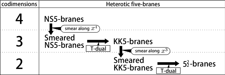
Figure 1: The smearing and the T-duality relations for the heterotic five-branes of various co-dimensions.

4 Monodromy and T-fold

In this section, we study the monodromy of the heterotic $5^{2}_{2}$-brane solutions. The T-duality symmetry in heterotic string theories compactified on $T^{d}$ with Wilson lines have been studied in detail [35, 36]. The Wilson line fields break the $SO(32)$ or $E_{8}\times E_{8}$ gauge group down to a Cartan subgroup of the gauge group. The off-diagonal parts of the Yang-Mills gauge field are Higgsed and becomes massive. In the lower-dimensions, there are $U(1)$ gauge fields which originate from the Kaluza-Klein reduction of the metric, the NS-NS $B$-field and the Yang-Mills gauge field that correspond to the Cartan subgroup. In this case, the T-duality group has been determined to be $O(d,d+\text{dim}G,\mathbb{R})$ where $\text{dim}G$ is the number of the $U(1)$ sector associated with the Cartan subgroup [37].

On the other hand, when the Wilson line fields are absent, the non-Abelian gauge group is not broken and the T-duality group $O(d,d+\text{dim}G,\mathbb{R})$ reduces to $O(d,d,\mathbb{R})$ [38]. Their study relies on the S-matrix analysis of strings and the result is true in all orders in $\alpha^{\prime}$. In order to clarify the $O(d,d)$ covariance of field configurations, it is convenient to consider the generalized metric $\mathcal{H}$. The generalized metric $\mathcal{H}$ in type II supergravity is a $2d\times 2d$ matrix and defined through the metric and the $B$-field. Although, the T-duality group $O(d,d)$ itself does not change for all orders in $\alpha^{\prime}$, the generalized metric receives $\alpha^{\prime}$-corrections. This is analogous to the $\alpha^{\prime}$-corrected Buscher rule of the T-duality transformation. Remarkably, in addition to the metric and the $B$-field, the Yang-Mills gauge field plays an important role in heterotic theories. The generalized metric in heterotic theories is determined by utilizing the heterotic supergravity action (1) compactified on $T^{d}$ [38]. This is given by

$$\mathcal{H}=\left[\begin{array}[]{cc}G^{-1}&-G^{-1}B\\ BG^{-1}&G-BG^{-1}B\end{array}\right],$$ (89)

where $G$ is defined by

$$G_{\mu\nu}=g_{\mu\nu}+2\alpha^{\prime}\bigl{[}\mbox{Tr}(\omega_{+\mu}\omega_{+\nu})-\mbox{Tr}(A_{\mu}A_{\nu})\bigr{]},$$ (90)

Here $\mu,\nu$ are the isometry directions. The generalized metric (89) takes the same form in type II supergravities but the second term in (90) is characteristic to heterotic theories. The spin connection term in (90) has been introduced as it enters into the action (1) in the same way as the Yang-Mills gauge field [38]. In the following, we investigate the monodromy structures of the heterotic $5^{2}_{2}$-branes by using the generalized metric (90).

Symmetric $5^{2}_{2}$-brane

For the symmetric $5^{2}_{2}$-brane, since the standard embedding condition is satisfied, we can choose a gauge where the second term in (90) is canceled. We find that the generalized metric is the same with the one in type II theory. For the solution (55), this is given by

$$\mathcal{H}(\theta)=\left[\begin{array}[]{cccc}H^{-1}K&0&0&H^{-1}\omega\\ 0&H^{-1}K&-H^{-1}\omega&0\\ 0&-H^{-1}\omega&HK^{-1}+(HK)^{-1}\omega^{2}&0\\ H^{-1}\omega&0&0&HK^{-1}+(HK)^{-1}\omega^{2}\end{array}\right].$$ (95)

When we go around the center of the $5^{2}_{2}$-brane and come back to the original point, namely if the angular position changes as $\theta=0\to 2\pi$, then the generalized metric is evaluated as

$$\mathcal{H}(2\pi)=O^{t}\mathcal{H}(0)O,$$ (96)

where

$$O=\left[\begin{array}[]{cc}-i\tau_{2}&0\\ 2\pi\sigma\mathbf{1}_{2}&-i\tau_{2}\end{array}\right]\in O(2,2).$$ (99)

This implies that the monodromy is given by the $O(2,2)$ T-duality transformation. Therefore, although the symmetric $5^{2}_{2}$-brane solution is non-geometric, it is a T-fold and a consistent solution to heterotic string theories.

Neutral $5^{2}_{2}$-brane

For the neutral $5^{2}_{2}$-brane, the bulk gauge field is trivial and we can always choose the gauge where $A_{M}=0$. Again, the modified spin connection is $\mathcal{O}(\alpha^{\prime})$ and it does not contribute to (90) and to the generalized metric. Then the generalized metric is given by (95) and its monodromy structure is the same with the symmetric case. Therefore we find that the neutral $5^{2}_{2}$-brane is a T-fold at least at $\mathcal{O}(\alpha^{\prime})$ in heterotic theories.

Gauge $5^{2}_{2}$-brane

For the gauge $5^{2}_{2}$-brane, the situation is different. The gauge field contributes to the generalized metric through (90) at $\mathcal{O}(\alpha^{\prime})$. However, since all the fields in the gauge solution do not depend on the angle $\theta$ in the two-dimensional base space, they do not inherit multi-valuedness of the geometry. Therefore the monodromy becomes trivial. This can be seen by evaluating the generalized metric for example in $\Theta=0$ gauge. In this gauge, we have

$$\mathcal{H}=\left[\begin{array}[]{cc}G^{-1}&0\\ 0&G\end{array}\right],\qquad G=e^{-2\phi_{0}}\mathbf{1}_{2}.$$ (102)

This implies $\mathcal{H}(2\pi)=\mathcal{H}(0)$. Therefore we concludes that the gauge $5^{2}_{2}$-brane does not exhibit non-geometric nature.

5 Conclusion and discussions

In this paper we studied the T-duality chains of five-branes in heterotic supergravity. A specific feature of heterotic supergravity is the Yang-Mills gauge sector which appears in the linear order in the $\alpha^{\prime}$-corrections. There are also higher derivative corrections of the curvature square term in the same order in $\alpha^{\prime}$. The three different half BPS five-brane solutions in this $\alpha^{\prime}$ order are known. They are the symmetric, the neutral and the gauge NS5-brane solutions. These are distinguished by the topological charge of instantons of Yang-Mills gauge field and the charge associated with the modified $H$-flux.

We introduced the $U(1)$ isometry along a transverse direction to the NS5-brane world-volume and explicitly performed the T-duality transformation of these solutions. Due to the $\alpha^{\prime}$-corrections in heterotic supergravity, the Buscher rule is modified by the corrections. For the symmetric solution, where the standard embedding condition is satisfied, the $\alpha^{\prime}$-corrections in the modified Buscher rule cancel out. The resulting metric, the $B$-field and the dilaton are nothing but the ones for the KK5-brane solution in type II theory. We demonstrated that the Yang-Mills gauge field satisfies the standard embedding condition again and it is given by the solution to the monopole equation in three dimensions. For the neutral solution, we find that the T-dualized solution is given by the KK5-brane in type II theory at least at $\mathcal{O}(\alpha^{\prime})$. The solution is given by the purely geometric Taub-NUT metric. For the gauge solution, the geometry is ill-defined near the brane core after the smearing procedure. This property is carried over to the T-dualized solution. For the gauge KK5-brane solution, the $B$-field is not excited which is the same with the KK5-brane in type II theory. However, the geometry is well-defined only at the asymptotic region.

We then introduce another $U(1)$ isometry to the KK5-brane solutions and perform the second T-duality transformation. The resulting solutions are the exotic $5^{2}_{2}$-branes in heterotic theory. For the symmetric solution, the metric, $B$-field and the dilation are given by that of the $5^{2}_{2}$-brane in type II theory. The gauge field satisfies the vortex-like equation in two dimensions. We found that the standard embedding condition is satisfied up to a gauge transformation. For the neutral solution, we found that the neutral $5^{2}_{2}$-brane is the same with the one in type II theory. They exhibit a non-geometric nature due to the multi-valuedness of the $B$-field. For the gauge $5^{2}_{2}$-brane solution, we found that the fields do not show the multi-valuedness and they remain geometric.

We next studied the monodromies of the three different $5^{2}_{2}$-branes. We calculated the generalized metric for these solutions. We found that the symmetric and the neutral $5^{2}_{2}$-branes have a monodromy given by the $O(2,2)$ T-duality transformation. Therefore they are T-folds. On the other hand, the gauge solution does not show the nature of a T-fold.

Following the general discussion in [34], the symmetric solution seems to be exact in terms of $\alpha^{\prime}$. On the other hand, for the neutral and the gauge $5^{2}_{2}$-brane solutions, they generically receive $\alpha^{\prime}$-corrections. The result is summarized in Table 1.

Type	Geometry	Valid order in $\alpha^{\prime}$	Notes
Symmetric	T-fold	$\alpha^{\prime}$-exact	standard embedding
Neutral	T-fold	$\mathcal{O}(\alpha^{\prime})$	Type II solution
Gauge	geometric	$\mathcal{O}(\alpha^{\prime})$	ill-defined near the center

Table 1: Properties of the heterotic $5^{2}_{2}$-branes.

A few comments are in order about the solutions. We introduced the $U(1)$ isometry to the gauge NS5-brane by the smearing procedure of the instantons. The resulting gauge field is just the Harrington-Shepard calorons in the small radius limit. The dilaton and the metric at $\mathcal{O}(\alpha^{\prime})$ are determined through the Bianchi identity $d\hat{H}^{(3)}=\alpha^{\prime}\mathrm{Tr}F\wedge F$ where the right-hand side is given by the topological charge density for the smeared caloron. The resulting geometry is ill-defined near the center of the brane. We stress that there is another co-dimension three solution based on the BPS monopole of ’t Hooft-Polyakov type instead of the smeared caloron [27, 29]. In the gauge NS5-brane solution of co-dimension three based on the BPS monopole type, the metric and the $B$-field behave well-defined near the core of the five-brane. The gauge KK5-and $5^{2}_{2}$-branes of BPS monopole type would show better physical interpretation of T-dualized solutions. A related property of the solutions is the logarithmic behaviour of the $5^{2}_{2}$-branes of all types. This is characteristic to the co-dimension two objects and found also in the solution in type II theory [15]. Similar to the gauge solutions of the smeared caloron type, the $5^{2}_{2}$-branes discussed in section 3.2 seem to be ill-defined at asymptotic region. However this does not indicate any inconsistency of the solutions but the general property of co-dimension two objects. Analogous to the D7-brane in type IIB string theory, the exotic $5^{2}_{2}$-brane is not well-defined as the stand-alone object. We need other co-existing branes in order to write down asymptotically flat globally well-defined solutions . Indeed, the scale $\mu$ in (52) specifies the “cutoff” point where the effect of the next duality branes is not negligible [31]. We believe that globally well-defined $5^{2}_{2}$-brane solutions exist even in heterotic theories.

We note that the most tractable way to study the non-geometric nature of string theory solutions is the double field theory construction of supergravity [40, 41]. There are several studies about double field theory formulation of heterotic supergravity [42] and the inclusion of $\alpha^{\prime}$-corrections [43]. Although the spin connection term in the generalized metric (90) is a conjectural one, the supersymmetry transformation law of the heterotic supergravity and the double field theory analysis strongly suggest that this is true [38]. Comprehensive studies are presented in the generalized geometry with $\alpha^{\prime}$-corrections [45]. The heterotic $5^{2}_{2}$-brane is expected to be a source of the non-geometric flux or mixed-symmetric tensor and they are in the T-duality multiplets in lower-dimensions [46]. It is also interesting to study the world-volume effective action for the non-geometric branes [47, 48] in heterotic theory. We will come back to these issues in future studies.

Acknowledgments

The authors would like to thank T. Kimura and S. Mizoguchi for useful discussions and comments. The work of S. S. is supported in part by Kitasato University Research Grant for Young Researchers. The work of M. Y. is supported by NUS Tier 1 FRC Grant R-144-000-316-112.

Appendix A Smeared solutions for gauge type

In this appendix, we introduce the explicit solutions of the smeared gauge KK5-brane. It is convenient first to introduce the defect gauge NS5-brane solution before we write down the smeared KK5-brane solution. The defect gauge NS5-brane solution is obtained by the smearing procedure along the $x^{4}$-direction to the $x^{3}$-smeared gauge NS5-brane. The resulting solution is a brane of co-dimension two. By performing the T-duality transformation along the $x^{3}$-direction, we obtain the $x^{4}$-smeared gauge KK5-brane.

A.1 Defect gauge NS5-brane solution

The defect gauge NS5-brane is the co-dimension two gauge NS5-brane and it is obtained by smearing the two directions of the gauge NS5-brane solution (34) along the same way to obtain the smeared gauge NS5-brane solution (48). The result is

$$ds^{2} =\eta_{ij}dx^{i}dx^{j}+{\cal I}\delta_{mn}dx^{m}dx^{n},~{}~{}~{}~{}~{}{\cal I}=e^{2\phi_{0}}-{\alpha^{\prime}\tilde{\sigma}^{2}\over 2r^{2}\bigl{(}\tilde{h}_{0}-{\tilde{\sigma}\over 2}\log(r/\mu)\bigr{)}^{2}},$$

$$A_{m} =-\bar{\sigma}_{mn}{\tilde{\sigma}x^{n}\over 4r^{2}\bigl{(}\tilde{h}_{0}-{\tilde{\sigma}\over 2}\log(r/\mu)\bigr{)}},~{}~{}~{}~{}\phi={1\over 2}\log{\cal I},~{}~{}~{}\hat{H}^{(3)}_{mnp}=-{1\over 2}\varepsilon_{mnpq}\partial_{q}{\cal I},$$ (103)

where $r^{2}=(x^{1})^{2}+(x^{2})^{2}$. In the gauge solution, since the non-zero components of the modified $H$-flux $\hat{H}_{mnp}$ come from the Yang-Mills Chern-Simons term, the $B$-field is taken to be a constant. For the defect NS5-brane solution, the relevant non-zero component of the $B$-field is $B_{34}=\Theta$. When we perform the heterotic T-duality transformation along the $x^{4}$-direction for the defect NS5-brane solution, we can obtain the smeared gauge KK5-brane solution shown below.

A.2 Smeared gauge KK5-brane solution

The smeared gauge KK5-brane solution is obtained by smearing $x^{3}$-direction in the gauge KK5-brane solution (86). The explicit form is as follows:

$$ds^{2} =\eta_{ij}dx^{i}dx^{j}+{\cal I}\delta_{m^{\prime}n^{\prime}}dx^{m^{\prime}}dx^{n^{\prime}}+{\cal I}e^{-4\phi_{0}}[dx^{4}+\Theta dx^{3}]^{2},$$

$$B_{MN} =0,~{}~{}~{}~{}~{}\phi={1\over 2}\log(e^{-2\phi_{0}}{\cal I}),~{}~{}~{}~{}~{}{\cal I}=e^{2\phi_{0}}-{\alpha^{\prime}\tilde{\sigma}^{2}\over 2r^{2}\bigl{(}\tilde{h}_{0}-{\tilde{\sigma}\over 2}\log(r/\mu)\bigr{)}^{2}},$$

$$A_{1} ={-\tilde{\sigma}x^{2}\over 4r^{2}\bigl{(}\tilde{h}_{0}-{\tilde{\sigma}\over 2}\log(r/\mu)\bigr{)}^{2}}T^{3},~{}~{}~{}~{}~{}A_{2}={\tilde{\sigma}x^{1}\over 4r^{2}\bigl{(}\tilde{h}_{0}-{\tilde{\sigma}\over 2}\log(r/\mu)\bigr{)}^{2}}T^{3},$$

$$A_{3} ={\tilde{\sigma}\over 4r^{2}\bigl{(}\tilde{h}_{0}-{\tilde{\sigma}\over 2}\log(r/\mu)\bigr{)}^{2}}\Bigl{(}(x^{2}T^{1}-x^{1}T^{2})+e^{-2\phi_{0}}\Theta(x^{1}T^{1}+x^{2}T^{2})\Bigr{)},$$

$$A_{4} =e^{-2\phi_{0}}{\tilde{\sigma}\over 4r^{2}\bigl{(}\tilde{h}_{0}-{\tilde{\sigma}\over 2}\log(r/\mu)\bigr{)}^{2}}(x^{1}T^{1}+x^{2}T^{2}).$$ (104)

As we mentioned above, the solution is obtained by taking the heterotic T-duality transformation along the $x^{4}$-direction on the defect gauge NS5-brane solution (103). When we take the heterotic T-duality transformation with the $x^{3}$-direction instead of the $x^{4}$-direction on (103), we find the other type of smeared gauge KK5-brane solution. The solution is different with the sign in front of $\Theta$ in (104), but the physical meanings are the same for both of the solutions. On the other hands, if we take the heterotic T-duality along the $x^{3}$-direction for the smeared gauge KK5-brane, we obtain the gauge $5^{2}_{2}$-brane solution as we see in (86).

References

- [1] C. M. Hull and P. K. Townsend, Nucl. Phys. B 438 (1995) 109 [hep-th/9410167].
- [2] S. Elitzur, A. Giveon, D. Kutasov and E. Rabinovici, Nucl. Phys. B 509 (1998) 122 [hep-th/9707217].
- [3] N. A. Obers and B. Pioline, Phys. Rept. 318 (1999) 113 [hep-th/9809039].
- [4] M. Blau and M. O’Loughlin, Nucl. Phys. B 525 (1998) 182 [hep-th/9712047].
- [5] E. Eyras and Y. Lozano, Nucl. Phys. B 573 (2000) 735 [hep-th/9908094].
- [6] E. Lozano-Tellechea and T. Ortin, Nucl. Phys. B 607 (2001) 213 [hep-th/0012051].
- [7] T. Kimura and S. Sasaki, Nucl. Phys. B 876 (2013) 493 [arXiv:1304.4061 [hep-th]], JHEP 1308 (2013) 126 [arXiv:1305.4439 [hep-th]], JHEP 1403 (2014) 128 [arXiv:1310.6163 [hep-th]].
- [8] T. Kimura, Nucl. Phys. B 893 (2015) 1 [arXiv:1410.8403 [hep-th]], arXiv:1503.08635 [hep-th], PTEP 2016 (2016) no.2, 023B04 [arXiv:1506.05005 [hep-th]], JHEP 1602 (2016) 013 [arXiv:1512.05548 [hep-th]], PTEP 2016 (2016) no.5, 053B05 [arXiv:1601.02175 [hep-th]], JHEP 1605 (2016) 060 [arXiv:1602.08606 [hep-th]].
- [9] D. Andriot and A. Betz, JHEP 1407 (2014) 059 [arXiv:1402.5972 [hep-th]].
- [10] T. Kimura, S. Sasaki and M. Yata, JHEP 1503 (2015) 076 [arXiv:1411.3457 [hep-th]],
- [11] E. A. Bergshoeff, T. Ortin and F. Riccioni, Nucl. Phys. B 856 (2012) 210 [arXiv:1109.4484 [hep-th]].
- [12] M. Park and M. Shigemori, JHEP 1510 (2015) 011 [arXiv:1505.05169 [hep-th]].
- [13] T. Okada and Y. Sakatani, JHEP 1503 (2015) 131 [arXiv:1411.1043 [hep-th]].
- [14] C. M. Hull, JHEP 0510 (2005) 065 [hep-th/0406102].
- [15] J. de Boer and M. Shigemori, Phys. Rev. Lett. 104 (2010) 251603 [arXiv:1004.2521 [hep-th]], Phys. Rept. 532 (2013) 65 [arXiv:1209.6056 [hep-th]].
- [16] F. Haßler and D. Lüst, JHEP 1307 (2013) 048 [arXiv:1303.1413 [hep-th]].
- [17] T. H. Buscher, Phys. Lett. B 194 (1987) 59, Phys. Lett. B 201 (1988) 466.
- [18] A. A. Tseytlin, Mod. Phys. Lett. A 6, 1721 (1991).
- [19] E. Bergshoeff, B. Janssen and T. Ortin, Class. Quant. Grav. 13 (1996) 321 [hep-th/9506156].
- [20] M. Serone and M. Trapletti, Phys. Lett. B 637 (2006) 331 [hep-th/0512272].
- [21] A. Strominger, Nucl. Phys. B 343 (1990) 167 Erratum: [Nucl. Phys. B 353 (1991) 565]
- [22] C. G. Callan, Jr., J. A. Harvey and A. Strominger, Nucl. Phys. B 359 (1991) 611, Nucl. Phys. B 367 (1991) 60.
- [23] M. J. Duff and J. X. Lu, Nucl. Phys. B 354 (1991) 141.
- [24] E. Bergshoeff and M. de Roo, Phys. Lett. B 218, 210 (1989), Nucl. Phys. B 328 (1989) 439.
- [25] A. A. Belavin, A. M. Polyakov, A. S. Schwartz and Y. S. Tyupkin, Phys. Lett. B 59 (1975) 85.
- [26] E. Witten, Nucl. Phys. B 460 (1996) 541 [hep-th/9511030].
- [27] R. R. Khuri, Nucl. Phys. B 387 (1992) 315 [hep-th/9205081].
- [28] A. P. Protogenov, Phys. Lett. 67B (1977) 62.
- [29] J. P. Gauntlett, J. A. Harvey and J. T. Liu, Nucl. Phys. B 409 (1993) 363 [hep-th/9211056].
- [30] B. J. Harrington and H. K. Shepard, Phys. Rev. D 17 (1978) 2122.
- [31] T. Kikuchi, T. Okada and Y. Sakatani, Phys. Rev. D 86 (2012) 046001 [arXiv:1205.5549 [hep-th]].
- [32] M. J. Duff and R. R. Khuri, Nucl. Phys. B 411 (1994) 473 [hep-th/9305142].
- [33] V. K. Onemli and B. Tekin, JHEP 0101 (2001) 034 [hep-th/0011287].
- [34] E. Bergshoeff, I. Entrop and R. Kallosh, Phys. Rev. D 49 (1994) 6663 [hep-th/9401025].
- [35] K. S. Narain, Phys. Lett. B 169 (1986) 41.
- [36] K. S. Narain, M. H. Sarmadi and E. Witten, Nucl. Phys. B 279 (1987) 369.
- [37] J. Maharana and J. H. Schwarz, Nucl. Phys. B 390 (1993) 3 [hep-th/9207016].
- [38] O. Hohm, A. Sen and B. Zwiebach, JHEP 1502 (2015) 079 [arXiv:1411.5696 [hep-th]].
- [39] B. R. Greene, A. D. Shapere, C. Vafa and S. T. Yau, Nucl. Phys. B 337 (1990) 1.
- [40] D. S. Berman and F. J. Rudolph, JHEP 1505 (2015) 015 [arXiv:1409.6314 [hep-th]].
- [41] I. Bakhmatov, A. Kleinschmidt and E. T. Musaev, arXiv:1607.05450 [hep-th].
- [42] O. Hohm and S. K. Kwak, JHEP 1106 (2011) 096 [arXiv:1103.2136 [hep-th]].
- [43] K. Lee, Nucl. Phys. B 899 (2015) 594 [arXiv:1504.00149 [hep-th]], O. Hohm, W. Siegel and B. Zwiebach, JHEP 1402 (2014) 065 [arXiv:1306.2970 [hep-th]], O. Hohm and B. Zwiebach, JHEP 1604 (2016) 101 [arXiv:1510.00005 [hep-th]], Phys. Rev. D 93 (2016) no.6, 064035 [arXiv:1509.02930 [hep-th]],
- [44] O. Hohm and B. Zwiebach, JHEP 1411 (2014) 075 [arXiv:1407.3803 [hep-th]], JHEP 1501 (2015) 012 [arXiv:1407.0708 [hep-th]], O. A. Bedoya, D. Marques and C. Nunez, JHEP 1412 (2014) 074 [arXiv:1407.0365 [hep-th]], D. Marques and C. A. Nunez, JHEP 1510 (2015) 084 [arXiv:1507.00652 [hep-th]], R. Blumenhagen and R. Sun, JHEP 1502 (2015) 097 [arXiv:1411.3167 [hep-th]].
- [45] A. Coimbra, R. Minasian, H. Triendl and D. Waldram, JHEP 1411 (2014) 160 [arXiv:1407.7542 [hep-th]].
- [46] E. A. Bergshoeff and F. Riccioni, JHEP 1301 (2013) 005 [arXiv:1210.1422 [hep-th]].
- [47] A. Chatzistavrakidis, F. F. Gautason, G. Moutsopoulos and M. Zagermann, Phys. Rev. D 89 (2014) 066004 [arXiv:1309.2653 [hep-th]].
- [48] T. Kimura, S. Sasaki and M. Yata, JHEP 1407 (2014) 127 [arXiv:1404.5442 [hep-th]], JHEP 1602 (2016) 168 [arXiv:1601.05589 [hep-th]].