33institutetext: School of Computer Science and Engineering, NTU, Singapore. 33email: ASJFCai@ntu.edu.sg
Improving Multi-label Learning with Missing Labels by
Structured Semantic Correlations
Abstract
Multi-label learning has attracted significant interests in computer vision recently, finding applications in many vision tasks such as multiple object recognition and automatic image annotation. Associating multiple labels to a complex image is very difficult, not only due to the intricacy of describing the image, but also because of the incompleteness nature of the observed labels. Existing works on the problem either ignore the label-label and instance-instance correlations or just assume these correlations are linear and unstructured. Considering that semantic correlations between images are actually structured, in this paper we propose to incorporate structured semantic correlations to solve the missing label problem of multi-label learning. Specifically, we project images to the semantic space with an effective semantic descriptor. A semantic graph is then constructed on these images to capture the structured correlations between them. We utilize the semantic graph Laplacian as a smooth term in the multi-label learning formulation to incorporate the structured semantic correlations. Experimental results demonstrate the effectiveness of the proposed semantic descriptor and the usefulness of incorporating the structured semantic correlations. We achieve better results than state-of-the-art multi-label learning methods on four benchmark datasets.
1 Introduction
Multi-label learning has been an important research topic in machine learning [1, 2, 3] and data mining [4, 5]. Unlike conventional classification problems, in multi-label learning each instance can be associated with multiple labels simultaneously. During recent years, multi-label learning has been applied on many computer vision tasks, especially on visual object recognition [6, 7, 8] and automatic image annotation [9, 10, 11]. In addition to the difficulty of assigning multiple labels/tags to complex images, multi-label learning often encounters the problem of incomplete labels. In real world scenarios, since the number of possible labels/tags is often very large (could be as large as the whole vocabulary set) and there often exist ambiguities among labels (e.g, “car” vs “SUV”), it is very difficult to obtain a perfectly labeled training set. Fig. 1 shows some examples of annotations from Flickr25K dataset. We can see that many possible labels are missing as it is impossible for labelers to go through the entire vocabulary set to extract all proper tags.


Due to the incompleteness nature of multi-label learning, many methods have been proposed to solve the problem of multi-label learning with missing labels. Most existing works focus on exploiting the correlations between features and labels (feature-label correlations) [12], the correlations between labels (label-label correlations) and the correlations between instances (instance-instance correlations) [1, 3, 13, 9]. Binary relevance (BR) [12] is a popular baseline for multi-label classification, which simply treats each class as a separate binary classification and makes use of feature-label correlations to solve the problem. However, its performance can be subpar as it ignores the correlations between labels and between instances. Several matrix completion based methods [14, 5, 3] handle the missing labels problem by implicitly exploiting label label correlations and instance-instance correlations with low-rank regularization on the label matrix. FastTag [13] also implicitly utilizes label-label correlations by learning an extra linear transformation on the label matrix to recover possible missing labels. On the other hand, LCML [1] explicitly handles missing labels with a probabilistic model.
Although these existing works exploit the correlations for learning classifiers and recovering missing labels, they generally (implicitly) assume that those correlations are linear and unstructured. However, in real world applications, especially image recognition, the label-label correlations and instance-instance correlations are actually structured. For example, label “landscape” is likely to co-exist with labels like “sky”, “mountain”, “river”, etc, but it is not likely to co-exist with “desk”, “computer”, “office”, etc. Deng et al. [15] already shows that the structured label correlations can benefit multi-class classification. In this work, we focus on exploiting the structured correlations between instances to improve multi-label learning. Given proper prior knowledge, our framework can also incorporate structured label correlations easily.
The key to utilize structured instance-instance correlations is to make use of semantic correlations between images, as semantically similar images should share similar labels. If we can effectively extract good semantic representations from images, we should be able to capture the structured correlations between instances.
A semantic representation of an image is a high level description of the image. One popular semantic representation is based on the score vectors of the classifier outputs. Many works have discussed the potential of such representations [16, 17, 18, 19, 20]. For example, Su and Jurie [20] proposed to use bag of semantics (BoS) to improve the image classification accuracy. Lampert et al. [19] employed semantics representations to describe objects by their attributes. Dixit et al. [17] combined CNN (convolutional neural networks) activations, semantic representations and Fisher vectors to improve scene classification. Kwitt et a. [18] also proposed to apply semantic representations on manifold for scene classification.
In this paper, we propose a new semantic representation, which is the concatenation of a global semantic descriptor and a local semantic descriptor. The global part of our semantic representation is similar to [17], which is the object-class posterior probability vector extracted from CNN trained with ILSVRC 2012 dataset. The global semantic descriptor describes “what is the image in general” according to a large number of concepts developed in the general large-scale dataset. We also introduce a local semantic descriptor extracted by averagely pooling the labels/tags of visual neighbors of each image in the specific target domain. The local semantic descriptor describes “what does the image specifically look like”. By combining the global and the local semantic descriptors, we achieve more accurate semantic representation.
With the accurate semantic descriptions of images, we propose to incorporate semantic instance-instance correlations to the multi-label learning problem by adding structures via graph. To be specific, after projecting the images into semantic space, we consider each semantic representation as a node and the whole image set as an undirected graph. Each edge of the graph connects two semantic image representations, and its weight represents the similarity between the node pair. We introduce the semantic graph Laplacian as a smooth term in the multi-label learning formulation to incorporate structured instance-instance correlations captured by the semantic graph. Experiments on four benchmark datasets demonstrate that by incorporating structured instance-instance semantic correlations, our proposed method significantly outperforms the state-of-the-art multi-label learning methods, especially at low observed rates of training labels (e.g. only observing of the given training labels). The major contributions of this paper lie in the proposed semantic representation and the proposed method to incorporate structured semantic correlations into multi-label learning.
2 Related Works on Multi-label Learning
Binary Relevance (BR) [12] is a standard baseline for multi-label learning, which treats each label as an independent binary classification. Linear or kernel classification tools such as LIBLINEAR [21] can then be applied to solve each binary classification subproblem. Although in general BR can achieve certain accuracy for multi-label learning tasks, it has two drawbacks. First of all, BR ignores the correlations between labels and between instances, which could be helpful for recognition. Secondly, as the label set size grows, the computational cost for BR in both training and testing becomes infeasible. To solve the first problem, some researchers proposed to estimate the label correlations from the training data. In particular, Hariharan et al. [22] and Petterson and Caetano [23] represent label dependencies by pairwise correlations computed from the training set, but such representations could be crude and inaccurate if the distribution of the training data is biased. LCML [1] uses a probability model to explicitly handle the label correlations. In multi-class classification, [15] exploits external label relation graph to model the correlations between labels. There also exist some works [4, 5, 14] that use the idea of matrix completion to implicitly deal with label correlations by imposing a nuclear norm to the formulation. To solve the second problem of BR, PLST [24] and CPLST [25] reduce the dimension of the label set by PCA related methods. Hsu et al. [26] employs a compressed sensing based approach to reduct the label set size. In addition to reducing label set size, these methods also decorrelate the labels, thus solving the first problem to a certain degree.
Nearest neighbors (NN) related methods are also commonly utilized in multi-label related applications. For label propagation, Kang et al. [27] proposed the Correlated label propagation (CLP) framework that propagates multiple labels jointly based on kNN methods. Yang et al. [28] utilized NN relationships as the label view in a multi-view multi-instance framework for multi-label object recognition. TagProp [29] combines metric learning and kNN to propagate labels. For tag refinement, Zhu et al. [30] proposed to use low-rank matrix completion formula with several graph constraints as the objective function to refine noisy or incomplete labels. For tag ranking, several methods [31, 32, 33] have been proposed to learn a ranking function utilizing the correlations between tags.
3 Problem Formulation
In the context of multi-label learning, let matrix refer to the true label (tag) matrix with rank , where is the number of instances and is the size of label set. As is generally not full-rank, without loosing generality, we can assume and . Given the data set , , where is the feature dimension of an instance. We make the following assumption:
Assumption 1
The column vectors in lie in the subspace spanned by the column vectors in .
Assumption 1 essentially means the label matrix can be accurately predicted by the linear combinations of the features of data set , which is the assumption generally used in linear classification [21, 14, 3]. Therefore, the goal of multi-label learning is to learn the linear projection such that it minimizes the reconstruction error:
| (1) |
where is the Frobenius norm.
Since the label matrix is generally incomplete in the real world applications, we assume to be the observed label matrix, where many entries are unknown. Let denote the set of the indices of the observed entries in , we can define a linear operator as
| (2) |
Then, the multi-label learning problem becomes: given and , how to find the optimal so that the estimated label matrix can be as close to the ground-truth label matrix as possible.
Similar to [14, 3], we can make use of the low-rank property of and optimize the following objective function:
| (3) |
where is the nuclear norm and is the tradeoff parameter. (3) is quintessentially the same as the matrix completion problem in [34].
Minimizing could be intractable for large-scale problems. If we assume that is orthogonal, which can be easily fulfilled by applying PCA to the original data set if it is not already orthogonal, we can reformulate (3) to
| (4) |
so that the problem can be solved much more efficiently [14].
The problem with (4) is that by employing the low rank condition, it implicitly assumes that rows/columns of label matrix is linearly dependent, i.e., the instance-instance correlations and label-label correlations are linear and unstructured. However, in real world applications, these correlations are actually structured. For example, [15] has already demonstrated that structured label-label correlations can benefit multi-class classification. In this work, we mainly consider the structured correlations among instances, but our framework can easily incorporate label-label correlations, if proper prior knowledge is available (such as the label relation graph in [15]).
To incorporate structured instance-instance correlations, we make one additional assumption:
Assumption 2
Semantically similar images should have similar labels.
It is reasonable to make this assumption as labels in multi-label image recognition problem can be viewed as a kind of semantic description of images. However, due to the limited label set size and missing labels problem, the observed labels are generally not precise enough. We will discussed this problem in detail in Section 4.
Assuming that we are able to accurately to project images to the semantic space, we can then incorporate structured instance-instance correlations based on Assumption 2. Specifically, an undirected weighted graph can be constructed with vertices (each vertex corresponds to the semantic representation of one image instance), edges , and the edge weight matrix that describes the similarity among image instances in semantic space. According to Assumption 2, the learned label matrix on the semantic graph should be smooth. To be specific, for any two instances , if they are semantically similar, i.e. the weight of edge on the semantic graph is large, their labels should also be similar, i.e., the distance between the learned labels of these two instances should be small. Thus, we define another regularization, aiming to minimize the distance between the learned labels of any two semantically similar instances:
| (5) |
where is the -th entry of the weight matrix .
(5) is equivalent to
| (6) |
where is the Laplacian of graph and . (6) is often referred as the Laplacian regularization term [35]. For simplicity, We use to represent to the Laplacian regularization on with respect to . We add this regularization term to the multi-label learning formulation to incorporate structured instance-instance correlations to the problem. In this way, the objective function of our multi-label learning with structured instance-instance correlations becomes:
| (7) |
where is the trade-off parameter.
If proper structured label-label correlations are available, we can also incorporate the information by adding another Laplacian regularization term on with the label correlation graph. Specifically, assuming we have an undirected graph with the weight matrix that captures the structured label-label correlations, we can similarly define the corresponding Laplacian regularization as
| (8) |
where is the Laplacian of the label correlation graph. However, unlike the label relation graph used in [15] for multi-class classification, the label correlations for multi-label learning are much more complicated and currently there is no such information available for multi-label learning, to the best of our knowledge. Therefore, in this paper, we stick to (7) as our optimization objective function.
The formulation of Zhu et al. [30] is closely related to ours, but with two key differences. Firstly, they focus on solving the tag refinement problem rather than classification. More importantly, our graph construction process is based on relationships in the semantic space with the proposed semantic descriptor rather than in the feature space, which we will describe in the following sections.
4 Semantic Descriptor Extraction
As we have discussed, if we are able to represent the image set with a semantic graph , we can incorporate structured instance-instance correlations to the multi-label learning problem. The problem now is: how to effectively project the images to the semantic space and build an appropriate semantic correlation graph.
For a multi-label learning problem, the labels of images can be viewed as semantic descriptions. However, since the size of the label set for many real-world applications is limited and more importantly the observed labels could be largely incomplete, using just the available labels as semantic descriptors would not be sufficient.
Previous works [16, 17, 19] make use of the posterior probabilities of the classifications on some general large-scale datasets such as ILSVRC 2012 [36] and Place database [37] with large number of classes as the semantic descriptors. In this paper, we also adopt such approach and utilize the score vector from CNN trained on ILSVRC 2012 as our global semantic descriptor. To better adapt the global descriptor to the target domain, we further develop feature selection to select most relevant semantic concepts. Moreover, we also propose to pool labels from visual neighbors of each instance in the target domain as the local semantic descriptor. The resulting overall semantic descriptor is empirically shown to have better discriminative power and stability over its individual components. In the following, we describe the details of the developed global and local semantic descriptors.
4.1 Global Semantic Descriptor
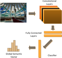
Given a vocabulary of semantic concepts, a semantic descriptor of image can be seen as the combination of these concepts, denoted as , . As the precise concept combination is not available, naturally we exploit the score vector extracted from the classifiers to describe the semantics of an image. Considering such semantic descriptor is essentially posterior class probabilities of a given image, we call it global semantic descriptor. Specifically, similar to [17], we apply CNN trained with ILSVRC 2012 and use the resulting posterior class probabilities as the global semantic vector. The process is illustrate in Fig. 2.
The problem with such global semantic vectors is that many semantic concepts in the source dataset might not be relevant to the target dataset. For example, if images from the target dataset are mainly related to animals, the responses of these images on some concepts such as man-made objects are generally not helpful and could even cause confusions. To eliminate such irrelevant or noisy concepts, we propose a simple feature selection method. Specifically, let’s denote the global semantic descriptions of a set of images with respect to concepts as , and their observed labels . We measure the relevance between semantic concept and the given label set as:
| (9) |
where evaluates the mutual information between and . essentially measures the accumulated linear dependency between concept and the given labels. After obtaining for all concepts, concepts are selected based on descending order of to preserve the most relevant concepts for the target dataset. The resulting global semantic descriptors for the target dataset is then denoted as .
4.2 Local Semantic Descriptor
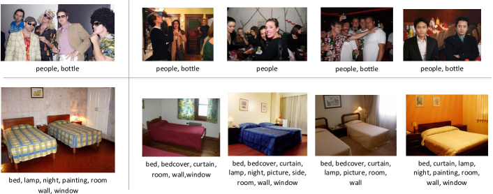
In addition to global semantic descriptor, we propose to extract local semantic descriptor to enhance the stability of the semantic descriptor and its relevance to target labels. Motivated by kNN classification, our basic idea is to utilize visual neighbors to generate local semantic descriptor. As illustrated in Fig. 3, the visual neighbors of an image are likely to share similar labels. If some labels of a particular image are missing, it is reasonable to assume that the observed labels of its visual neighbors can be helpful to approximate the semantic description of the image. Therefore, we include labels of visual neighbors as part of our proposed semantic descriptor.
To be specific, for an image , we search for its top- visual neighbors, which have observed labels . The local semantic descriptor of is defined as
| (10) |
(10) is essentially an average pooling of labels , which tells “what does the image look like”. By find for all images, we can form a set of local semantic descriptors for the target dataset. The final semantic descriptor set is the direct concatenation of and , denoted as and .
4.3 Graph Construction
After extracting the semantic descriptor set , we can now construct the semantic correlation graph based on . In particular, we treat each semantic representation as a node of the undirected graph in the semantic space. To effectively construct the edges between node and other nodes, following the general idea of [38], we first search for neighbors in the semantic space of , which we refer as semantic neighbors. Note that the number of semantic neighbors can be different from the number of visual neighbors that we use for building local semantic descriptors. We then connect and its semantic neighbors to form the edges from . The weight of an edge is defined as the dot-product between its two nodes, i.e.,
| (11) |
The complete process for constructing the semantic correlation graph is summarized in Algorithm 1.
5 Proximal Gradient Descent Based Solver
Solving our objective function (7) is not straightforward, although it is convex, the nuclear norm is non-smooth. Following [39, 14], we employ an accelerated proximal gradient (APG) method to solve the problem.
We first consider minimizing the smooth loss function without the nuclear norm regularization:
| (12) |
A well-known fact [40] is that the gradient step
| (13) |
for solving the smooth problem can be formulated as a proximal regularization of the linearized function at as
| (14) |
where
denotes the matrix inner product, and is the step size of iteration .
Based on the above derivation, following [39], (7) is then solved by the following iterative optimization:
| (15) |
Further ignoring the terms that do not dependent on , we simplify (15) into minimizing
| (16) |
which can be solved by singular value thresholding (SVT) techniques [41].
Algorithm 2 shows the APG method we used for solving (7). Similar to [14], we introduce an auxiliary variable (line ) to accelerate the convergence. At each step, by utilizing the Lipschitz continuity of the gradient of , the step size can be found in an iterative fashion. Specifically, we start from a constant and iteratively increase until the following condition is met:
| (17) |
which is equivalent to line 6 in Algorithm 2.
6 Experimental Results
In this section, we compare our proposed APG-Graph algorithm with several state-of-the-art methods on four widely used multi-label learning benchmark datasets. The details of the benchmark datasets can be found in Table 1. We follow the pre-defined split of train and test111 http://lear.inrialpes.fr/people/guillaumin/data.php. To mimic the effect of missing labels, we uniformly sample of labels from each class of the train set, where . It means we only use of the training labels. We use mean average precision (mAP) as our evaluation metric, which is the mean of average precision across all labels/tags of the test set and is widely used in multi-label learning.
NUS-WIDE is also widely used as multi-label classification benchmark dataset. Unfortunately, we cannot obtain all the images from NUS-WIDE dataset. Since we are unable to extract the semantic descriptors without original images, we cannot perform experiments in this dataset.
| Dataset | #Train | #Test | #Labels | #Avg Labels |
|---|---|---|---|---|
| VOC 2007 | 5011 | 4952 | 20 | 1.4 |
| ESP Game | 18689 | 2081 | 268 | 4.5 |
| Flickr 25K | 12500 | 12500 | 38 | 4.7 |
| IAPRTC-12 | 17665 | 1962 | 291 | 5.7 |
6.1 Experiment Setup
Feature representation for input data : For all the image instances (train and test), we need to find their effective feature representations as the input data . Note that for simplicity, we abuse the notation for both the input image set and the corresponding image description set. In particular, we employ the 16-layer very deep CNN model in [42]. We apply the CNN pre-trained on ILSVRC 2012 dataset to each image and use the activations of the -th layer as the visual descriptor (-dimensional) of the image. We then concatenate the semantic descriptor developed in Algorithm 1 with this -dimensional visual descriptor as the overall feature representation for image . To satisfy our Assumption 2, we further apply PCA to the overall feature representations to decorrelate the features. The dimension of PCA features is set to preserve energy of the original features, which results in the final descriptor of dimensions around .
Finding visual neighbors: To find accurate visual neighbors for local semantic descriptor, we extract a low-dimensional CNN descriptor for each image. We use the same 16-layer very deep CNN structure, except that the activations of the -th fully connected layer is of dimensions instead of . The -d descriptors denoted as are used to find visual neighbors as described in Section 4.2.
Baselines: We compare our method with the following baselines.
-
Maxide [14]: A matrix completion based multi-label learning method using training data as side information to speed up the training process. Although the formulation of Maxide incorporate a label correlation matrix, while in experiments Maxide actually sets it as identity matrix. Maxide outperforms other matrix completion based methods like MC- and MC-b [4, 9]. The formulation of Maxide is similar to our formulation without the Laplacian regularization term.
-
FastTag [13]: A fast image tagging algorithm based on the assumption of uniformly corrupted labels. FastTag learns an extra transformation on the label matrix to recover its missing entries. It achieves state-of-the-art performances on several benchmark datasets.
-
Least Squares: LS is a a ridge regression model which uses the partial subset of labels to learn the decision parameter .
We cross-validate the parameters of these methods on smaller subsets of benchmark datasets to ensure best performance.
Our parameters: The learning part of our method has two parameters and as shown in (7). Similar to other methods, we cross-validate on a small subset of benchmark datasets to get the best parameters. The parameters for the semantic correlation graph construction are decided empirically. Specifically, the number of semantic concepts used in global semantic descriptors is set to be . The number of visual neighbors is set to be and the number of semantic neighbors is set to be .
6.2 Validation of Semantic Descriptor
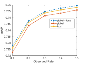
We validate the effectiveness of the proposed semantic descriptor on Flickr25K dataset by demonstrating the classification accuracy. As shown in Fig. 4, for the recognition rate on the test set, our proposed global + local descriptor has the highest mAP consistently. The gain over just using local semantic descriptor is not so large though. We suspect that since the global semantic descriptors are extracted from ILSVRC dataset, which is an object dataset, and the tags of Flickr25K are mostly not related to objects, the global semantic descriptor is not so helpful in this case. If we use other sources of global semantic vocabulary more related to scene, e.g., Place database, we could potentially have even better performance.
6.3 Comparison with Other Methods
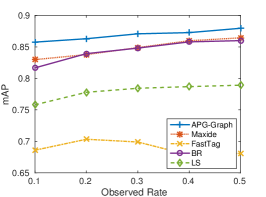
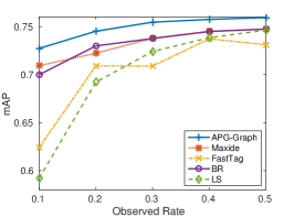
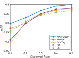
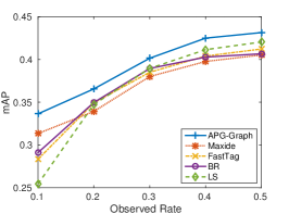
Fig. 5 shows the mAP results of our proposed method and the four baselines on the four benchmark datasets. It can be seen that our method (APG-Graph) constantly outperforms other methods, especially when the observed rate is small. The performance gain validates the effectiveness of our proposed semantic descriptors and the usage of structured instance-instance correlation. On the other hand, Maxide generally achieves similar recognition rate as BR for observed rates ranging from to while it outperforms BR at an observed rate of , which suggests that the unstructured correlation enforced by the low-rank constraint (nuclear norm) is helpful at small observed rates, but the effect is similar to the L norm used in SVM classification at large observed label rates. We use the code provided by [13] for FastTag. It seems that FastTag is not very effective in our experiments, especially for datasets with fewer labels (VOC2007 and Flickr25K). We suspect that the hyper-parameter tuning in FastTag is not stable when the labels are fewer. We also show some examples of recognized images in Fig. 6.
Note that other methods such as TagProp [29] and TagRelevance [43] are not designed for our problem setting and cannot handle missing labels properly, thus in our preliminary experiments their results are bad and we choose not to report them.

7 Conclusion
In this paper, we have incorporated structured semantic correlations to solve the missing label problem of multi-label learning. Specifically, we project images to the semantic space with an effective semantic descriptor. A semantic graph is then constructed on these images to capture the structured correlations between images. We utilize the semantic graph Laplacian as a smooth term in the multi-label learning formulation to incorporate these correlations. Experimental results demonstrate the effectiveness of our proposed multi-label learning framework as well as our proposed semantic representation. Future works could include utilizing other large scale datasets such as Place as another source of global semantic concepts and incorporating structured label correlations.
Acknowledgments This research is supported by Singapore MoE AcRF Tier-1 Grant RG138/14 and also partially by Rolls-Royce@NTU Corportate Lab Project C-RT3.5. The Tesla K40 used for this re-search was donated by the NVIDIA Corporation.
References
- [1] Bi, W., Kwok, J.T.: Multilabel classification with label correlations and missing labels. In: AAAI. (2014) 1680–1686
- [2] Liu, M., Luo, Y., Tao, D., Xu, C., Wen, Y.: Low-rank multi-view learning in matrix completion for multi-label image classification. In: AAAI. (2015) 2778–2784
- [3] Yu, H., Jain, P., Kar, P., Dhillon, I.S.: Large-scale multi-label learning with missing labels. In: ICML. (2014) 593–601
- [4] Kong, X., Ng, M.K., Zhou, Z.: Transductive multilabel learning via label set propagation. IEEE TKDE 25(3) (2013) 704–719
- [5] Kong, X., Wu, Z., Li, L., Zhang, R., Yu, P.S., Wu, H., Fan, W.: Large-scale multi-label learning with incomplete label assignments. In: SDM. (2014) 920–928
- [6] Everingham, M., Gool, L., Williams, C.K., Winn, J., Zisserman, A.: The Pascal Visual Object Classes (VOC) challenge. IJCV 88(2) (June 2010) 303–338
- [7] Gong, Y., Jia, Y., Leung, T., Toshev, A., Ioffe, S.: Deep convolutional ranking for multilabel image annotation. CoRR abs/1312.4894 (2013)
- [8] Oquab, M., Bottou, L., Laptev, I., Sivic, J.: Learning and transferring mid-level image representations using convolutional neural networks. In: CVPR. (2014) 1717–1724
- [9] Cabral, R.S., la Torre, F.D., Costeira, J.P., Bernardino, A.: Matrix completion for multi-label image classification. In: NIPS. (2011) 190–198
- [10] Tariq, A., Foroosh, H.: Feature-independent context estimation for automatic image annotation. In: CVPR. (2015) 1958–1965
- [11] Wang, Q., Shen, B., Wang, S., Li, L., Si, L.: Binary codes embedding for fast image tagging with incomplete labels. In: ECCV. (2014) 425–439
- [12] Tsoumakas, G., Katakis, I.: Multi-label classification: An overview. IJDWM 3(3) (2007) 1–13
- [13] Chen, M., Zheng, A.X., Weinberger, K.Q.: Fast image tagging. In: ICML. (2013) 1274–1282
- [14] Xu, M., Jin, R., Zhou, Z.: Speedup matrix completion with side information: Application to multi-label learning. In: NIPS. (2013) 2301–2309
- [15] Deng, J., Ding, N., Jia, Y., Frome, A., Murphy, K., Bengio, S., Li, Y., Neven, H., Adam, H.: Large-scale object classification using label relation graphs. In: ECCV. (2014) 48–64
- [16] Bergamo, A., Torresani, L.: Classemes and other classifier-based features for efficient object categorization. IEEE TPAMI 36(10) (2014) 1988–2001
- [17] Dixit, M., Chen, S., Gao, D., Rasiwasia, N., Vasconcelos, N.: Scene classification with semantic fisher vectors. In: CVPR. (2015) 2974–2983
- [18] Kwitt, R., Vasconcelos, N., Rasiwasia, N.: Scene recognition on the semantic manifold. In: ECCV. (2012) 359–372
- [19] Lampert, C.H., Nickisch, H., Harmeling, S.: Attribute-based classification for zero-shot visual object categorization. IEEE TPAMI 36(3) (2014) 453–465
- [20] Su, Y., Jurie, F.: Improving image classification using semantic attributes. IJCV 100(1) (2012) 59–77
- [21] Fan, R., Chang, K., Hsieh, C., Wang, X., Lin, C.: LIBLINEAR: A library for large linear classification. JMLR 9 (2008) 1871–1874
- [22] Hariharan, B., Zelnik-Manor, L., Vishwanathan, S.V.N., Varma, M.: Large scale max-margin multi-label classification with priors. In: ICML. (2010) 423–430
- [23] Petterson, J., Caetano, T.S.: Submodular multi-label learning. In: NIPS. (2011) 1512–1520
- [24] Tai, F., Lin, H.: Multilabel classification with principal label space transformation. Neural Computation 24(9) (2012) 2508–2542
- [25] Chen, Y., Lin, H.: Feature-aware label space dimension reduction for multi-label classification. In: NIPS. (2012) 1538–1546
- [26] Hsu, D., Kakade, S., Langford, J., Zhang, T.: Multi-label prediction via compressed sensing. In: NIPS. (2009) 772–780
- [27] Kang, F., Jin, R., Sukthankar, R.: Correlated label propagation with application to multi-label learning. In: CVPR. (2006) 1719–1726
- [28] Yang, H., Zhou, J.T., Zhang, Y., bin Gao, B., Wu, J., Cai, J.: Exploit bounding box annotations for multi-label object recognition. In: CVPR. (2016) 280–288
- [29] Guillaumin, M., Mensink, T., Verbeek, J.J., Schmid, C.: Tagprop: Discriminative metric learning in nearest neighbor models for image auto-annotation. In: IEEE 12th International Conference on Computer Vision, ICCV 2009, Kyoto, Japan, September 27 - October 4, 2009. (2009) 309–316
- [30] Zhu, G., Yan, S., Ma, Y.: Image tag refinement towards low-rank, content-tag prior and error sparsity. In: Proceedings of the 18th International Conference on Multimedia 2010, Firenze, Italy, October 25-29, 2010. (2010) 461–470
- [31] Liu, D., Hua, X., Yang, L., Wang, M., Zhang, H.: Tag ranking. In: Proceedings of the 18th International Conference on World Wide Web, WWW 2009, Madrid, Spain, April 20-24, 2009. (2009) 351–360
- [32] Jeong, J., Hong, H., Lee, D.: ikang2006-tagranker: an efficient tag ranking system for image sharing and retrieval using the semantic relationships between tags. Multimedia Tools Appl. 62(2) (2013) 451–478
- [33] Zhuang, J., Hoi, S.C.H.: A two-view learning approach for image tag ranking. In: Proceedings of the Forth International Conference on Web Search and Web Data Mining, WSDM 2011, Hong Kong, China, February 9-12, 2011. (2011) 625–634
- [34] Candès, E.J., Recht, B.: Exact matrix completion via convex optimization. Foundations of Computational Mathematics 9(6) (2009) 717–772
- [35] Ando, R.K., Zhang, T.: Learning on graph with laplacian regularization. In: NIPS. (2006) 25–32
- [36] Russakovsky, O., Deng, J., Su, H., Krause, J., Satheesh, S., Ma, S., Huang, Z., Karpathy, A., Khosla, A., Bernstein, M., Berg, A.C., Fei-Fei, L.: ImageNet Large Scale Visual Recognition Challenge. IJCV (April 2015) 1–42
- [37] Zhou, B., Lapedriza, À., Xiao, J., Torralba, A., Oliva, A.: Learning deep features for scene recognition using places database. In: NIPS. (2014) 487–495
- [38] Belkin, M., Niyogi, P., Sindhwani, V.: Manifold regularization: A geometric framework for learning from labeled and unlabeled examples. JMLR 7 (2006) 2399–2434
- [39] Ji, S., Ye, J.: An accelerated gradient method for trace norm minimization. In: ICML. (2009) 457–464
- [40] Bertsekas, D.P.: Nonlinear Programming. Athena Scientific, Belmont, MA (1999)
- [41] Cai, J.F., Candès, E.J., Shen, Z.: A singular value thresholding algorithm for matrix completion. SIAM J. on Optimization 20(4) (March 2010) 1956–1982
- [42] Simonyan, K., Zisserman, A.: Very deep convolutional networks for large-scale image recognition. CoRR abs/1409.1556 (2014)
- [43] Li, X., Snoek, C.G.M., Worring, M.: Learning social tag relevance by neighbor voting. IEEE Transactions on Multimedia 11(7) (2009) 1310–1322