Gradient recovery for elliptic interface problem: I. body-fitted mesh

Abstract

In this paper, we propose a novel gradient recovery method for elliptic interface problem using body-fitted mesh in two dimension. Due to the lack of regularity of solution at interface, standard gradient recovery methods fail to give superconvergent results, and thus will lead to overrefinement when served as a posteriori error estimator. This drawback is overcome by designing an immersed gradient recovery operator in our method. We prove the superconvergence of this method for both mildly unstructured mesh and adaptive mesh, and present several numerical examples to verify the superconvergence and its robustness as a posteriori error estimator.

1 Introduction

Elliptic interface problem frequently appears in the fields of fluid dynamics and material science, where background consists of rather different materials. The numerical challenge comes from discontinuities of coefficient at interface, where solution is not smooth in general. Computational methods for elliptic interface problem have been studied intensively in literature, which can be roughly categorized into two types: unfitted mesh methods and body-fitted mesh methods.

Numerical methods based on unfitted mesh solve interface problems on Cartesian grids, among which, famous examples include immersed boundary method (IBM) by Peskin [35, 36] and immersed interface method (IIM) by Leveque and Li [24], just to name a few. We refer interested readers to [26] for a review of the literature. IBM uses Dirac $\delta$-function to model discontinuity and discretizes it to distribute a singular source to nearest grid point. IIM constructs a special finite difference scheme near interface to get an accurate approximation of the solution. It was further developed in the framework of finite element method [25, 27, 28], which modifies basis functions on interface elements. Moreover, in [20, 21], a special weak form was derived based on Petro-Galerkin method to discretize elliptic interface problem. A shortcoming of unfitted mesh methods is that, the resulting discretized linear system is in general non-symmetric and indefinite even thought the original continuous problem is self-adjoint.

Body-fitted mesh methods require mesh grids to align with interface in order to capture discontinuity. The resulting discretized linear system is symmetric and positive definite if the original continuous problem is self-adjoint. Error estimates for finite element method with body-fitted mesh have been established by [2, 6, 13, 42]. In particular, [13] showed that smooth interface can be approximated by linear interpolation of distinguished points on interface. Although the solution to interface problem has low global regularity, the finite element approximation was shown to have nearly the same optimal error estimates in both $L^{2}$ and energy norms as for regular (non-interface) problems.

Meanwhile, superconvergence analysis has attracted considerable attention in the community of finite element method, and theories have been well developed for regular problems [3, 10, 39, 47]. Then it is natural to ask if one can obtain similar superconvergence results for elliptic interface problem. However, limited work has been done in this direction due to the lack of regularity of solution at interface. Recently, [14, 15] proposed two special interpolation formula to recover flux for linear and quadratic immersed finite element method in one dimension. Supercloseness was established between finite element solution and linear interpolation of the true solution in [40].

In this paper, we aim to develop gradient recovery methods for elliptic interface problem based on body-fitted finite element discretization. Standard gradient recovery operators, including superconvergent patch recovery (SPR) [48, 49] and polynomial preserving recovery (PPR) [44, 32, 33], produce superconvergent recovered gradient only when the solution is smooth enough. Therefore, they can not be applied directly to elliptic interface problem since the solution has low regularity at the interface due to the discontinuity of coefficients. Futuremore, building up a recovery-type a posteriori error estimator based on these methods will lead to overrefine regions as studied in [8].

An observation that we rely on is that, even though the solution has low global regularity, it is piecewise smooth on each subdomain separated by the smooth interface. This motivates us to develop a novel gradient recovery method by applying PPR gradient operator on each subdomain since PPR is a local gradient recovery method. One one hand, for a node away from interface, we use stand PPR gradient recovery operator; On the other hand, for a node close to interface, we design the gradient recovery operator by fitting a quadratic polynomial in least-squares sense only using the sampling points in each subdomain. This will generate two approximations of gradient in each subdomain for a node on interface, which is consistent with the fact that the solution in general is not continuously differentiable at interface. The method is more like to use a divide-and-conquer strategy, which has also been used in the immersed finite element method [25, 27, 28].

We prove that the proposed gradient recovery method has superconvergence for the following two types of meshes: Benefited from [40] on the approximation estimate and supercloseness, we are able to establish the superconvergence theory on mildly unstructured meshes; Using the practical assumption and supercloseness results in [41] for adaptive mesh, we show that the proposed recovered gradient method is superconvergent to exact gradient on adaptive mesh. Therefore, the method provides an asymptotically exact a posteriori error estimator for elliptic interface problem. Compared to the a posteriori error estimator in [4, 12, 30] and recovery-type error estimator in [8, 9], the estimator based on the proposed gradient recovery is easier in implementation and asymptotically more exact, which will be verified by several two-dimensional numerical examples.

The rest of the paper is organized as follows. In Section 2, we introduce elliptic interface problem and its finite element approximation based on body-fitted mesh. In Section 3, we first give a brief introduction to polynomial preserving recovery method, based on which, we develop a novel gradient recovery method for elliptic interface problem. In Section 4, superconvergence is proved for the proposed gradient recovery operator on both mildly unstructured mesh and adaptive refined mesh. In addition, we show that the method provides an asymptotically exact a posteriori error estimator for elliptic interface problem. In Section 5, serval numerical examples are presented to confirm our theoretical results. Conclusive remarks are made in Section 6.

2 Finite element method for elliptic interface problem

In this section, we first introduce elliptic interface problem, and then describe the finite element approximation using body-fitted mesh.

2.1 Elliptic interface problem

Let $\Omega$ be a bounded polygonal domain with Lipschitz boundary $\partial\Omega$ in $\mathbb{R}^{2}$. A $C^{2}$-curve $\Gamma$ divides $\Omega$ into two disjoint subdomains $\Omega^{-}$ and $\Omega^{+}$, which is typically characterized by zero level set of some level set function $\phi$ [34, 38]. Then $\Omega^{-}=\{z\in\Omega|\phi(z)<0\}$ and $\Omega^{+}=\{z\in\Omega|\phi(z)>0\}$. We shall consider the following elliptic interface problem

$$-\nabla\cdot(\beta(z)\nabla u(z)) =f(z),\quad z\text{ in }\Omega\setminus\Gamma,$$ (2.1)

$$u =0,\quad\quad\,\,z\text{ on }\partial\Omega,$$ (2.2)

where the diffusion coefficient $\beta(z)\geq\beta_{0}$ is a piecewise smooth function, i.e.

$$\beta(z)=\left\{\begin{array}[]{ccc}\beta^{-}(z)&\text{if }z\in\Omega^{-},\\ \beta^{+}(z)&\text{if }z\in\Omega^{+},\end{array}\right.$$ (2.3)

which has a finite jump of function values across the interface $\Gamma$. At the interface $\Gamma$, one has the following jump conditions

$$[u]_{\Gamma} =u^{+}-u^{-}=0,$$ (2.4)

$$[\beta u_{n}]_{\Gamma} =\beta^{+}u_{n}^{+}-\beta^{-}u^{-}_{n}=g,$$ (2.5)

where $u_{n}$ denotes the normal flux $\nabla u\cdot n$ with $n$ as the unit outer normal vector of the interface $\Gamma$.

Notations. Let $C$ denote a generic positive constant which may be different at different occurrences. For the sake of simplicity, we use $x\lesssim y$ to mean that $x\leq Cy$ for some constant $C$ independent of mesh size. Standard notations for Sobolev spaces and their associate norms given in [7, 16, 19] are adopted in this paper. Moreover, for a subdomain $A$ of $\Omega$, let $\mathbb{P}_{m}(A)$ be the space of polynomials of degree less than or equal to $m$ in $A$ and $n_{m}$ be the dimension of $\mathbb{P}_{m}(A)$ which equals to $\frac{1}{2}(m+1)(m+2)$. $W^{k,p}(A)$ denotes the Sobolev space with norm $\|\cdot\|_{k,p,A}$ and seminorm $|\cdot|_{k,p,A}$. When $p=2$, $W^{k,2}(A)$ is simply denoted by $H^{k}(A)$ and the subscript $p$ is omitted in its associate norm and seminorm. As in [40], denote $W^{k,p}(\Omega^{-}\cup\Omega^{+})$ as the function space consisting of piecewise Sobolev function $w$ such that $w|_{\Omega^{-}}\in W^{k,p}(\Omega^{-})$ and $w|_{\Omega^{+}}\in W^{k,p}(\Omega^{+})$. For the function space $W^{k,p}(\Omega^{-}\cup\Omega^{+})$, define norm as

$$\|w\|_{k,p,\Omega^{-}\cup\Omega^{+}}=\left(\|w\|_{k,p,\Omega^{-}}^{p}+\|w\|_{k,p,\Omega^{+}}\right)^{1/p},$$

and seminorm as

$$|w|_{k,p,\Omega^{-}\cup\Omega^{+}}=\left(|w|_{k,p,\Omega^{-}}^{p}+|w|_{k,p,\Omega^{+}}\right)^{1/p}.$$

The variational formulation of elliptic interface problem equations 2.1, 2.2, 2.4 and 2.5 is given by finding $u\in H^{1}_{0}(\Omega)$ such that

$$(\beta\nabla u,\nabla v)=(f,v)-\langle g,v\rangle,\quad\forall v\in H^{1}_{0}(\Omega),$$ (2.6)

where $(\cdot,\cdot)$ and $\langle g,v\rangle$ are standard $L_{2}$-inner product in the spaces $L^{2}(\Omega)$ and $L^{2}(\Gamma)$ respectively. By the positiveness of $\beta$, Lax-Milgram Theorem implies equation 2.6 has a unique solution. [13, 37] proved that $u\in H^{r}(\Omega^{-}\cup\Omega^{+})$ for $0\leq r\leq 2$ and

$$\|u\|_{r,\Omega^{-}\cup\Omega^{+}}\lesssim\|f\|_{0,\Omega}+\|g\|_{r-3/2,\Gamma},$$ (2.7)

if $f\in L^{2}(\Omega)$ and $g\in H^{r-3/2}(\Gamma)$.

Remark 1.

For the sake of easing theoretical analysis, we simply assume homogeneous jump of function value. In fact, one can extend the method to inhomogeneous jump of function value $[u]_{\Gamma}=q$ by defining a piecewise smooth function $\hat{q}$ that satisfies $\hat{q}|_{\Gamma}=q$ and $\hat{q}|_{\partial\Omega}=0$, and then the problem equations 2.1, 2.2 and 2.5 is equivalent to find $u=w+\hat{q}$ with $w\in H^{1}_{0}(\Omega)$ such that

$$(\beta\nabla w,\nabla v)=(f,v)-\langle g,v\rangle-(\beta\nabla\hat{q},\nabla v),\quad\forall v\in H^{1}_{0}(\Omega).$$

2.2 Finite element approximation

Denote $\mathcal{T}_{h}$ to be a body-fitted triangulation of $\Omega$, then every triangle $T\in\mathcal{T}_{h}$ belongs to one of the following three different cases:

1. $T\subset\overline{\Omega^{-}}$;

2. $T\subset\overline{\Omega^{+}}$;

3. $T\cap\Omega^{-}\neq\emptyset$ and $T\cap\Omega^{-}\neq\emptyset$, then two of vertices of $T$ lie on $\Gamma$.

For any $T\in\mathcal{T}_{h}$, denote its diameter and supermum of the diameters of the circles inscribed in $T$ by $h_{T}$ and $\rho_{T}$ respectively. Let $h=\max_{T\in\mathcal{T}_{h}}h_{T}$. Assume that the triangulation of $\Omega$ is shape-regular in the sense that there is a constant $\xi$ such that $\frac{h_{T}}{\rho_{T}}\leq\xi$ for all $T\in\mathcal{T}_{h}$. Denote $\Gamma_{h}$ as an approximation to $\Gamma$ which consists of the edges with both endpoints lying on $\Gamma$. The domain $\Omega$ is divided into two parts $\Omega^{-}_{h}$ and $\Omega^{+}_{h}$ by $\Gamma_{h}$, which are the approximation of $\Omega^{-}$ and $\Omega^{+}$ respectively.

The element in $\mathcal{T}_{h}$ can be categorized into two types: regular elements and interface elements. An element $T$ is called interface element if it has exactly two vertices on $\Gamma$; otherwise, it is called regular element. The set of all interface elements is denoted by $\mathcal{T}_{h}^{*}$. For each element $T\in\mathcal{T}_{h}^{*}$, let $T^{-}=T\cap\Omega^{-}$ and $T^{+}=T\cap\Omega^{+}$. Since $\Gamma$ is $C^{2}$, one has

$$|T^{-}|\lesssim h^{3}_{T},\text{ or }|T^{+}|\lesssim h^{3}_{T},$$

as shown in [13].

For each edge $e$ on $\Gamma_{h}$, define a projection $\mathcal{P}_{h}$ [6, 40] from $e$ to $\Gamma$ as

$$\mathcal{P}_{h}(z)=z+d(z)n_{h},\quad\forall z\in e,$$ (2.8)

where $n_{h}$ is the unit normal vector of $e$ pointing from $\Omega^{-}$ to $\Omega^{+}$ and $d(z)$ is the sign distance function between $z$ and $\Gamma$ along $n_{h}$. Note that $\mathcal{P}_{h}$ is a point in $\Gamma$ for each $z\in e$. According to [40, 6], the projection $\mathcal{P}_{h}$ and its inverse are well defined when the length of $e$ is small enough.

Let $V_{h}$ be the continuous linear finite element space and $V_{h,0}=V_{h}\cap H^{1}_{0}(\Omega)$. We approximate the diffusion coefficient $\beta$ by $\beta_{h}$ with $\beta_{h}|_{T}=\beta^{-}$ if $T\in\Omega^{-}_{h}$ and $\beta_{h}|_{T}=\beta^{+}$ if $T\in\Omega^{+}_{h}$. Then the linear finite element approximation of the variational problem equation 2.6 is to find $u_{h}\in V_{h,0}$ such that

$$(\beta_{h}\nabla u_{h},\nabla v_{h})=(f,v_{h})-\langle g_{h},v_{h}\rangle_{\Gamma_{h}},\quad\forall v_{h}\in V_{h,0},$$ (2.9)

where $g_{h}=g(P_{h}(z))$ and $\langle\cdot,\cdot\rangle$ is $L^{2}$-inner product of $L^{2}(\Gamma_{h})$. Moreover, [13, 42, 45] proved the following convergence results for the finite element approximation (2.9).

Theorem 2.1.

Let $u$ and $u_{h}$ be the solution to equation 2.6 and equation 2.9 respectively, then we have

$$\|\nabla u-\nabla u_{h}\|_{0,\Omega}\lesssim h|\log h|^{1/2}(\|f\|_{0,\Omega}+\|g\|_{2,\Gamma}),$$ (2.10)

$$\|u-u_{h}\|_{0,\Omega}\lesssim h^{2}|\log h|^{1/2}(\|f\|_{0,\Omega}+\|g\|_{2,\Gamma}).$$ (2.11)

Note that the error estimate equation 2.10 is nearly optimal due to the existence of $|\log h|^{1/2}$.

3 Gradient recovery for elliptic interface problem

In this section, we first summarize the polynomial preserving recovery(PPR) method proposed by Zhang and Naga in [44, 32, 33] for finite element approximation of standard elliptic problem, then based on which, we propose a novel gradient recovery method for elliptic interface problem.

3.1 Polynomial preserving recovery

For any vertex $z$ and $n\in\mathbb{Z}^{+}$, let $\mathcal{L}(z,n)$ denote the union of elements in the first $n$ layers around $z$, i.e.,

$$\mathcal{L}(z,n):=\bigcup\left\{\tau:\tau\in\mathcal{T}_{h},\tau\cap\mathcal{L}(z,n-1)\neq\emptyset\right\},$$ (3.1)

where $\mathcal{L}(z,0):=\{z\}$.

The set of all mesh vertices and edges are denoted by $\mathcal{N}_{h}$ and $\mathcal{E}_{h}$ respectively. The standard Lagrange basis of $V_{h}$ is denoted by $\{\phi_{z}:z\in\mathcal{N}_{h}\}$ with $\phi_{z}(z^{\prime})=\delta_{zz^{\prime}}$ for all $z,z^{\prime}\in\mathcal{N}_{h}$. Let us introduce $G_{h}:V_{h}\rightarrow V_{h}\times V_{h}$ as the PPR gradient recovery operator. For any vertex $z$, let $\mathcal{K}_{z}$ be a patch of elements around $z$. Select all nodes in $\mathcal{N}_{h}\cap\mathcal{K}_{z}$ as sampling points and fit a polynomial $p_{z}\in\mathbb{P}_{k+1}(\mathcal{K}_{z})$ in the least square sense at those sampling points, i.e.

$$p_{z}=\arg\min_{p\in\mathbb{P}_{k+1}(\mathcal{K}_{z})}\sum_{\tilde{z}\in\mathcal{N}_{h}\cap\mathcal{K}_{z}}(u_{h}-p)^{2}(\tilde{z}).$$ (3.2)

Then the recovered gradient at $z$ is defined as

$$(G_{h}u_{h})(z)=\nabla p_{z}(z).$$

After obtaining recovered gradient value at all nodal points, we define recovered gradient $G_{h}$ on the whole domain by

$$G_{h}u_{h}:=\sum_{z\in\mathcal{N}_{h}}(G_{h}u_{h})(z)\phi_{z}.$$ (3.3)

Remark 2.

If $u_{h}$ is a function in $V_{h}$, then $\nabla u_{h}$ is a piecewise constant function and hence is discontinuous on $\Omega$. However, the recovered gradient $G_{h}u_{h}$ is a continuous piecewise linear function. In that sense, $G_{h}$ can be viewed as a smoothing operator to smooth a discontinuous piecewise constant function into a continuous piecewise linear function.

To complete the definition of PPR, one needs to define $\mathcal{K}_{z}$. If $z$ is an interior vertex, $\mathcal{K}_{z}$ is defined as the smallest $\mathcal{L}(z,n)$ that guarantees the uniqueness of $p_{z}$ in (3.2) [44, 32, 33]. In the case that $z\in\mathcal{N}_{h}\cup\partial\Omega$, let $n_{0}$ be the smallest positive integer such that $\mathcal{L}(z,n_{0})$ has at least one interior mesh vertex. Then, we define

$$\mathcal{K}_{z}=\mathcal{L}(z,n_{0})\cup\{\mathcal{K}_{\tilde{z}}:\tilde{z}\in\mathcal{L}(z,n_{0})\text{ and }\tilde{z}\text{ an interior vertex}\}.$$

Remark 3.

In order to avoid numerical instability, a discrete least squares fitting process is carried out on a reference patch $\omega_{z}$.

The PPR gradient recovery operator $G_{h}$ has the following properties, as proved in [44, 32, 33]:

1. $G_{h}$ is a linear operator.

2. $G_{h}$ preserves quadratic polynomials. Consequently, $G_{h}$ enjoys the approximation property

   $$\|\nabla u-G_{h}u_{I}\|\lesssim h^{2}|u|_{3,\Omega},\quad\forall u\in H^{3}(\Omega),$$ (3.4)

   where $u_{I}$ is the linear interpolation of $u$ in $V_{h}$.

3. $\|G_{h}v_{h}\|_{0,\Omega}\lesssim\|\nabla v_{h}\|_{0,\Omega},\forall v_{h}\in V_{h}$.

3.2 Immersed polynomial preserving recovery operator

As we mentioned in 2, standard PPR can be viewed a smoothing operator. However, $\nabla u$ is discontinuous across the interface $\Gamma$ in elliptic interface problem, and thus standard PPR won’t work since it provides continuous gradient approximation. Noticing that, although $u$ have low global regularity due to existence of interface, $u|_{\Omega^{-}}$ (or $u|_{\Omega^{+}}$) is smooth, which motivates us to recover piecewise continuous gradient approximation instead.

Let $\Omega_{h}$ be a body-fitted triangulation introduced in Subsection 2.2. The approximate interface $\Gamma_{h}$ divides the triangulation $\Omega_{h}$ into two disjoint sets:

$$\mathcal{T}^{-}_{h}:=\left\{T\in\mathcal{T}_{h}|\text{ all three vertices of }T\text{ are in }\overline{\Omega^{-}}\right\},$$ (3.5)

$$\mathcal{T}^{+}_{h}:=\left\{T\in\mathcal{T}_{h}|\text{ all three vertices of }T\text{ are in }\overline{\Omega^{+}}\right\}.$$ (3.6)

Let $V_{h}^{-}$ and $V_{h}^{-}$ be the continuous linear finite element spaces defined on $\mathcal{T}_{h}^{-}$ and $\mathcal{T}_{h}^{+}$ respectively.

Denote the PPR gradient recovery operator on $V_{h}^{-}$ by $G_{h}^{-}$. Then $G_{h}^{-}$ is a linear bounded operator from $V_{h}^{-}$ to $V_{h}^{-}\times V_{h}^{-}$. Similarly, let $G_{h}^{+}$ be PPR gradient recovery operator from $V_{h}^{+}$ to $V_{h}^{+}\times V_{h}^{+}$. Then, for any $u_{h}\in V_{h}$, we choose the global gradient recovery operator $G_{h}^{I}:V_{h}\rightarrow(V_{h}^{-}\cup V_{h}^{+})\times(V_{h}^{-}\cup V_{h}^{+})$ as

$$(G_{h}^{I}u_{h})(z)=\left\{\begin{array}[]{ccc}(G_{h}^{-}u_{h})(z)&\text{if }z\in\overline{\Omega^{-}_{h}},\\ (G_{h}^{+}u_{h})(z)&\text{if }z\in\overline{\Omega^{+}_{h}}.\end{array}\right.$$ (3.7)

Specifically, we define $(G_{h}^{I}u_{h})(z)$ according to the location of $z$:

• If $z$ is far from the approximate interface $\Gamma_{h}$, $(G_{h}^{I}u_{h})(z)$ is the standard PPR gradient recovery at $z$.

• If $z$ is close to the approximate interface $\Gamma_{h}$, $(G_{h}^{I}u_{h})(z)$ is given by fitting a quadratic polynomial using sampling points only from $\mathcal{T}_{h}^{-}$ or only from $\mathcal{T}_{h}^{+}$.

• If $z$ is on approximate interface $\Gamma_{h}$, $(G_{h}^{I}u_{h})(z)$ is given by two values: one by $(G_{h}^{-}u_{h})(z)$ and the other by $(G_{h}^{+}u_{h})(z)$.

We call $G_{h}^{I}$ as immersed polynomial preserving recovery (IPPR) operator.

Remark 4.

Given a function $u_{h}$ in $V_{h}$, $G_{h}^{I}u_{h}$ is not a function in $V_{h}\times V_{h}$, since it is two-valued on the approximate interface $\Gamma_{h}$ as described in Case 3.

Remark 5.

The choice of $G_{h}^{I}$ is not limited to PPR gradient recovery operator, and in fact it can be any local gradient recovery operator such as weighted averaging gradient recovery operator [1] and SPR gradient recovery operator [48, 49]. One can also use different gradient recovery operators on two subdomains separated by $\Gamma_{h}$, for example, PPR gradient recovery operator on $V_{h}^{-}$ and SPR gradient recovery operator on $V_{h}^{+}$. We shall use PPR gradient recovery operator in this paper for convenience.

Remark 6.

The IPPR operator can be generalized to the case when the domain $\Omega$ is divided into serval subdomains by defining the gradient recovery operator piecewisely in each subdomain.

Moreover, we have the following approximation estimate for the IPPR gradient recovery operator $G_{h}^{I}$.

Theorem 3.1.

Let $G_{h}^{I}:V_{h}\rightarrow(V_{h}^{-}\cup V_{h}^{+})\times(V_{h}^{-}\cup V_{h}^{+})$ be the IPPR gradient recovery operator. Given $u\in H^{3}(\Omega^{-}\cup\Omega^{+})$, then

$$\|G_{h}^{I}u_{I}-\nabla u\|_{0,\Omega}\lesssim h^{2}\|u\|_{3,\Omega^{-}\cup\Omega^{+}},$$ (3.8)

where $u_{I}$ is interpolation of $u$ into linear finite element space $V_{h}$.

Proof.

Notice that $G_{h}^{-}$ and $G_{h}^{+}$ are the standard PPR gradient recovery operators. Formula equation 3.4 implies that

$$\|G_{h}^{-}u_{I}-\nabla u\|_{0,\Omega_{h}^{-}}\lesssim h^{2}\|u\|_{3,\Omega^{-}},\text{ and }\|G_{h}^{+}u_{I}-\nabla u\|_{0,\Omega_{h}^{+}}\lesssim h^{2}\|u\|_{3,\Omega^{+}}.$$

Therefore,

$$\|G_{h}^{I}u_{I}-\nabla u\|^{2}_{0,\Omega} =\|G_{h}^{-}u_{I}-\nabla u\|_{0,\Omega_{h}^{-}}^{2}+\|G_{h}^{+}u_{I}-\nabla u\|_{0,\Omega_{h}^{+}}^{2}$$

$$\lesssim h^{4}\|u\|_{3,\Omega^{-}}^{2}+h^{4}\|u\|_{3,\Omega^{+}}^{2}$$

$$\lesssim h^{4}\|u\|_{3,\Omega^{-}\cup\Omega^{+}}.$$

∎

4 Superconvergence Analysis

In this section, we prove that the IPPR gradient recovery method has superconvergence for both mildly unstructured mesh and adaptive mesh.

4.1 Superconvergence on mildly unstructured mesh

We first introduce a definition on mesh structure.

Definition 4.1.

1. Two adjacent triangles are called to form an $\mathcal{O}(h^{1+\alpha})$ approximate parallelogram if the lengths of any two opposite edges differ only by $\mathcal{O}(h^{1+\alpha})$.

2. The triangulation $\mathcal{T}_{h}$ is called to satisfy Condition $(\sigma,\alpha)$ if there exist a partition $\mathcal{T}_{h,1}\cup\mathcal{T}_{h,2}$ of $\mathcal{T}_{h}$ and positive constants $\alpha$ and $\sigma$ such that every two adjacent triangles in $\mathcal{T}_{h,1}$ form an $\mathcal{O}(h^{1+\alpha})$ parallelogram and

$$\sum_{T\in{\mathcal{T}_{h,2}}}|T|=\mathcal{O}(h^{\sigma}).$$

Under the above mesh condition, the following supercloseness result holds:

Theorem 4.2.

Let $u$ be the solution to variational problem equation 2.6 and $u_{h}$ be the finite element solution to equation 2.9. If the body-fitted mesh satisfies Condition $(\sigma,\alpha)$ and $u\in H^{1}(\Omega)\cap H^{3}(\Omega^{-}\cup\Omega^{+})\cap W^{2,\infty}(\Omega^{-}\cup\Omega^{+})$, then for any $v_{h}\in V_{h,0}$,

$$\begin{split}(\beta_{h}\nabla(u-u_{I}),\nabla v_{h})\lesssim&h^{1+\rho}(\|u\|_{3,\Omega^{-}\cup\Omega^{+}}+\|u\|_{2,\infty,\Omega^{-}\cup\Omega^{+}})|v_{h}|_{1,\Omega}\\ &+h^{\frac{3}{2}}\|u\|_{2,\infty,\Omega^{-}\cup\Omega^{+}}|v_{h}|_{1,\Omega},\end{split}$$ (4.1)

and

$$\begin{split}\|\nabla(u_{I}-u_{h})\|_{0,\Omega}\lesssim&h^{1+\rho}(\|u\|_{3,\Omega^{-}\cup\Omega^{+}}+\|u\|_{2,\infty,\Omega^{-}\cup\Omega^{+}})\\ &+h^{\frac{3}{2}}(\|u\|_{2,\infty,\Omega^{-}\cup\Omega^{+}}+\|g\|_{0,\infty,\Gamma}),\end{split}$$ (4.2)

where $\rho=\min(\alpha,\frac{\sigma}{2},\frac{1}{2})$ and $u_{I}\in V_{h}$ is the interpolation of $u$.

Proof.

The proof is similar to the proof of Theorem 3.6 in [40] where one uses the estimates in [43] instead of [11]. ∎

Remark 7.

If $\Gamma=\Gamma_{h}$ or the flux jump $g$ given by (2.5) vanishes with $\Gamma$ smooth enough so that $|T^{-}|\lesssim h^{4}_{T}$ ( or $|T^{+}|\lesssim h^{4}_{T}$ ), then one has the following $O(h^{1+\rho})$ superconvergence results

$$\begin{split}(\beta_{h}\nabla(u-u_{I}),\nabla v_{h})\lesssim&h^{1+\rho}(\|u\|_{3,\Omega^{-}\cup\Omega^{+}}+\|u\|_{2,\infty,\Omega^{-}\cup\Omega^{+}})|v_{h}|_{1,\Omega},\end{split}$$ (4.3)

and

$$\begin{split}\|\nabla(u_{I}-u_{h})\|_{0,\Omega}\lesssim&h^{1+\rho}(\|u\|_{3,\Omega^{-}\cup\Omega^{+}}+\|u\|_{2,\infty,\Omega^{-}\cup\Omega^{+}}).\end{split}$$ (4.4)

Remark 8.

The difference between theorem 4.2 and Theorem 3.6 in [40] lies in the condition on mesh structure. The $\mathcal{O}(h^{2\sigma})$ irregular mesh in [40] is a special case of Condition $(\sigma,\alpha)$.

Remark 9.

For body-fitted mesh generated by Delaunay algorithm, the assumption that two adjacent triangles form $\mathcal{O}(h^{1+\alpha})$ approximate parallelogram is violated near boundary and interface, however, the summation of area of such triangles is bounded by $\mathcal{O}(h^{\sigma})$, and thus it Condition $(\sigma,\alpha)$.

The supercloseness result in theorem 4.2 implies the following superconvergent result.

Theorem 4.3.

Under the same hypothesis as in Theorem 4.2, then we have

$$\begin{split}\|\nabla u-G_{h}^{I}u_{h}\|_{0,\Omega}\lesssim&h^{1+\rho}(\|u\|_{3,\Omega^{-}\cup\Omega^{+}}+\|u\|_{2,\infty,\Omega^{-}\cup\Omega^{+}})+\\ &h^{\frac{3}{2}}(\|u\|_{2,\infty,\Omega^{-}\cup\Omega^{+}}+\|g\|_{0,\infty,\Gamma}),\end{split}$$ (4.5)

where $\rho=\min(\alpha,\frac{\sigma}{2},\frac{1}{2})$.

Proof.

We decompose $\nabla u-G_{h}^{I}u_{h}$ as $(\nabla u-G_{h}^{I}u_{I})-(G_{h}^{I}u_{I}-G_{h}^{I}u_{h})$, and then by triangle inequality,

$$\begin{split}&\|\nabla u-G_{h}^{I}u_{h}\|_{0,\Omega}\\ \leq&\|\nabla u-G_{h}^{I}u_{I}\|_{0,\Omega}+\|G_{h}^{I}u_{I}-G_{h}^{I}u_{h}\|_{0,\Omega}\\ \leq&\|\nabla u-G_{h}^{I}u_{I}\|_{0,\Omega}+\|G_{h}^{-}u_{I}-G_{h}^{-}u_{h}\|_{0,\Omega_{h}^{-}}+\|G_{h}^{+}u_{I}-G_{h}^{+}u_{h}\|_{0,\Omega_{h}^{+}}\\ \leq&\|\nabla u-G_{h}^{I}u_{I}\|_{0,\Omega}+\|\nabla(u_{I}-u_{h}))\|_{0,\Omega_{h}^{-}}+\|\nabla(u_{I}-u_{h})\|_{0,\Omega_{h}^{+}}\\ \leq&\|\nabla u-G_{h}^{I}u_{I}\|_{0,\Omega}+\|\nabla(u_{I}-u_{h})\|_{0,\Omega},\\ \end{split}$$ (4.6)

where we have used boundedness of PPR gradient recovery operator $G_{h}^{-}$ and $G_{h}^{+}$. The first term can be bounded by Theorem 3.1 and the second term is estimated in Theorem 4.2, which completes the proof. ∎

Remark 10.

Under the same assumptions in 7, one has the following improved superconvergence results

$$\begin{split}\|\nabla u-G_{h}^{I}u_{h}\|_{0,\Omega}\lesssim&h^{1+\rho}(\|u\|_{3,\Omega^{-}\cup\Omega^{+}}+\|u\|_{2,\infty,\Omega^{-}\cup\Omega^{+}}).\end{split}$$ (4.7)

4.2 Superconvergence on adaptive mesh

In this subsection, for simplicity, we assume that the interface $\Gamma$ does not cut through any element $T\in\mathcal{T}_{h}$, i.e. $\Gamma=\Gamma_{h}$, which implies $\Omega^{-}=\Omega^{-}_{h}$ and $\Omega^{+}=\Omega^{+}_{h}$. Furthermore, we assume that the solution $u$ to equation 2.6 has a single singularity on the interface $\Gamma$, and without loss of generality, we assume that the singularity is at the origin and $u^{-}$ (or $u^{+}$) can be decomposed into a smooth part $w^{-}$ (or $w^{+}$) and singular part $v^{-}$ (or $v^{+}$), i.e.,

$$u^{-}=w^{-}+v^{-},\text{ and }u^{+}=w^{+}+v^{+},$$ (4.8)

where

$$\left|\frac{\partial^{m}w^{-}}{\partial x^{i}\partial y^{m-i}}\right|\lesssim 1,\text{ and }\left|\frac{\partial^{m}v^{-}}{\partial x^{i}\partial y^{m-i}}\right|\lesssim r^{\delta-m},$$ (4.9)

and

$$\left|\frac{\partial^{m}w^{+}}{\partial x^{i}\partial y^{m-i}}\right|\lesssim 1,\text{ and }\left|\frac{\partial^{m}v^{+}}{\partial x^{i}\partial y^{m-i}}\right|\lesssim r^{\delta-m},$$ (4.10)

with $r=\sqrt{x^{2}+y^{2}}$ and $0<\delta<2$ being a constant.

For any edge $e$ of the mesh $\mathcal{T}_{h}$, let $h_{e}$ be the length of the edge and $r_{e}$ be the distance from the origin to the midpoint of $e$. If $e$ is an interior edge, denote $\Omega_{e}$ to be the patch of $e$ consisting of two triangles sharing the edge $e$. In addition, let $\underline{h}\simeq\min_{T\in\mathcal{T}_{h}}h_{T}$ and $N$ be the number of vertices of $\mathcal{T}_{h}$. To get superconvergence, one also needs the following restriction on mesh structure.

Definition 4.4.

The triangulation $\mathcal{T}_{h}$ is called to satisfy Condition $(\alpha,\sigma,\mu)$ if there exist constants $\alpha>0$, $\sigma\geq 0$, and $\mu>0$ such that the interior edge can separated into two parts $\mathcal{E}_{h}=\mathcal{E}_{1,h}\oplus\mathcal{E}_{2,h}$: $\Omega_{e}$ forms an $\mathcal{O}\left(h^{1+\alpha}_{e}/r_{e}^{\alpha+\mu(1-\alpha)}\right)$ parallelogram for $\forall e\in\mathcal{E}_{1,h}$ and the number of edges in $\mathcal{E}_{2,h}$ satisfies $\#\mathcal{E}_{2,h}\lesssim N^{\sigma}$.

Note that the above mesh condition is a practical assumption for adaptive mesh as shown in [41]. In addition, we assume $h_{T}\simeq r_{T}^{1-\mu}\underline{h}^{\mu}$ for any $T\in\mathcal{T}_{h}$, and then we can establish the following supercloseness result on adaptive mesh.

Theorem 4.5.

Let $u$ be the solution to variational problem equation 2.6 and $u_{h}$ be the finite element solution to equation 2.9. Suppose adaptive refined mesh $\mathcal{T}_{h}$ satisfies Condition $(\alpha,\sigma,\delta/2)$, and $h_{T}\simeq r_{T}^{1-\delta/2}\underline{h}^{\delta/2}$ for any $T\in\mathcal{T}_{h}$, then for any $v_{h}\in V_{h,0}$,

$$(\beta_{h}\nabla(u-u_{I}),\nabla v_{h})\lesssim\frac{1+(\ln N)^{1/2}}{N^{1/2+\rho}}\|\nabla v_{h}\|_{0,\Omega},$$ (4.11)

and

$$\begin{split}\|\beta^{1/2}(\nabla u_{I}-\nabla u_{h})\|_{0,\Omega}\lesssim&\frac{1+(\ln N)^{1/2}}{N^{1/2+\rho}}\|\nabla v_{h}\|_{0,\Omega},\end{split}$$ (4.12)

where $\rho=\min\left(\frac{\alpha}{2},\frac{1-\sigma}{2}\right)$ and $u_{I}$ is the linear interpolation of $u$.

Proof.

First, one can decompose $(\beta_{h}\nabla(u-u_{I}),\nabla v_{h})$ as

$$\begin{split}&(\beta_{h}\nabla(u-u_{I}),\nabla v_{h})\\ =&(\beta^{-}(\nabla u^{-}-u_{I}^{-}),\nabla v_{h})_{\Omega^{-}}+(\beta^{+}(\nabla u^{+}-u_{I}^{+}),\nabla v_{h})_{\Omega^{+}}\\ =&I_{1}+I_{2}.\end{split}$$

Lemma 3.3 in [41] implies the following estimates for $I_{1}$ and $I_{2}$,

$$\begin{split}I_{1}\lesssim&\frac{1+(\ln N)^{1/2}}{N^{1/2+\rho}}\|\nabla v_{h}\|_{0,\Omega},\\ I_{2}\lesssim&\frac{1+(\ln N)^{1/2}}{N^{1/2+\rho}}\|\nabla v_{h}\|_{0,\Omega},\end{split}$$

which completes the proof of equation 4.11. By equations 2.6 and 2.9 and noticing that $\Gamma=\Gamma_{h}$ and $\beta=\beta_{h}$, we have

$$(\beta_{h}\nabla(u_{I}-u_{h}),\nabla v_{h})=(\beta_{h}\nabla(u_{I}-u),\nabla v_{h}).$$

Taking $v_{h}=u_{I}-u_{h}$ gives equation 4.12. ∎

Before presenting our main superconvergent theorem on adaptive refined mesh, we need to estimate gradient recovery operator analogous to Theorem 3.1.

Theorem 4.6.

Assume that $h_{T}\simeq r_{T}^{1-\delta/2}\underline{h}^{\delta/2}$ for any $T\in\mathcal{T}_{h}$, then

$$\|\nabla u-G_{h}^{I}u_{I}\|_{0,\Omega}\lesssim\frac{1+(\ln N)^{1/2}}{N}.$$ (4.13)

Proof.

The definition of $G_{h}^{I}$ produces

$$\|\nabla u-G_{h}^{I}u_{I}\|_{0,\Omega}^{2}=\|\nabla u^{-}G_{h}^{-}u_{I}^{-}\|_{0,\Omega^{-}}^{2}+\|\nabla u^{+}-G_{h}^{+}u_{I}^{+}\|_{0,\Omega^{+}}^{2}.$$ (4.14)

Note that $u^{-}$ (or $u^{+}$) has the decomposition equation 4.8 and $G_{h}^{-}$ (or $G_{h}^{+}$ ) is the standard PPR gradient recovery operator. Lemma 5.2 in [41] implies

$$\|\nabla u^{-}-G_{h}^{-}u_{I}^{-}\|_{0,\Omega^{-}}\lesssim \frac{1+(\ln N)^{1/2}}{N},$$ (4.15)

$$\|\nabla u^{+}-G_{h}^{+}u_{I}^{+}\|_{0,\Omega^{+}}\lesssim \frac{1+(\ln N)^{1/2}}{N}.$$ (4.16)

Combing equations 4.14, 4.15 and 4.16 gives equation 4.13. ∎

Then we can prove the superconvergence as follows.

Theorem 4.7.

Let $u$ be the solution to variational problem equation 2.6 and $u_{h}$ be the finite element solution to equation 2.9. If the adaptive refined mesh $\mathcal{T}_{h}$ satisfies Condition $(\alpha,\sigma,\delta/2)$ and $h_{T}\simeq r_{T}^{1-\delta/2}\underline{h}^{\delta/2}$ for any $T\in\mathcal{T}_{h}$, then

$$\|\beta^{1/2}(\nabla u-G_{h}^{I}u_{h})\|_{0,\Omega}\lesssim\frac{1+(\ln N)^{1/2}}{N^{1/2+\rho}},$$ (4.17)

where $\rho=\min\left(\frac{\alpha}{2},\frac{1-\sigma}{2}\right)$.

Proof.

The proof is essentially the same as in Theorem 4.3 where one should use Theorems 4.6 and 4.5 instead of Theorems 3.1 and 4.2. ∎

Using the IPPR gradient recovery operator $G_{h}^{I}$, one can define a local a posteriori error estimator on element $T\in\mathcal{T}_{h}$ as

$$\eta_{T}=\|\beta^{1/2}(G_{h}^{I}u_{h}-\nabla u_{h})\|_{0,T},$$ (4.18)

and the corresponding global error estimator as

$$\eta_{h}=\left(\sum_{T\in\mathcal{T}_{h}}\eta_{T}^{2}\right)^{1/2}.$$ (4.19)

Theorem 4.7 implies that $\eta_{h}$ is asymptotically exact a posteriori error estimator for elliptic interface problem.

Theorem 4.8.

Let $u$ be the solution to variational problem equation 2.6 and $u_{h}$ be the finite element solution to equation 2.9. Suppose adaptive refined mesh $\mathcal{T}_{h}$ satisfies Condition $(\alpha,\sigma,\delta/2)$ and $h_{T}\simeq r_{T}^{1-\delta/2}\underline{h}^{\delta/2}$ for any $T\in\mathcal{T}_{h}$, and if

$$\frac{1}{N^{1/2}}\lesssim\|\beta^{1/2}(\nabla(u-u_{h}))\|_{0,\Omega},$$ (4.20)

then

$$\left|\frac{\eta_{h}}{\|\beta^{1/2}(\nabla u-\nabla u_{h})\|_{0,\Omega}}-1\right|\lesssim\frac{1+(\ln N)^{1/2}}{N^{\rho}},$$ (4.21)

where $\rho=\min\left(\frac{\alpha}{2},\frac{1-\sigma}{2}\right)$.

Remark 11.

Assumption equation 4.20 is reasonable according to lower bounded estimates of approximation by finite element spaces [23, 29].

5 Numerical Examples

In this section, we present serval numerical examples to illustrate the superconvergence of the IPPR gradient recovery method and confirm the theoretical results given in the previous section. We also make numerical comparison to standard PPR method [32, 33, 44] to show the effectiveness. For convenience, we shall use the following error measurements in all examples:

$$De := \|u-u_{h}\|_{1,\Omega},\quad\quad\quad D^{i}e:=\|\nabla u_{I}-\nabla u_{h}\|_{0,\Omega},$$ (5.1)

$$D^{r}e := \|\nabla u-G^{I}_{h}u_{h}\|_{0,\Omega},\quad D^{p}e:=\|\nabla u-G_{h}u_{h}\|_{0,\Omega}.$$ (5.2)

Remark that all convergence rate will be computed in the degree of freedom (Dof), and since $\text{Dof}\approx h^{-2}$ for a two-dimensional quasi-uniform mesh, the corresponding convergent rate in mesh size $h$ is twice as much as what we present in the tables.

Example 5.1. In this example, we consider the elliptic interface problem equation 2.1 with a circular interface of radius $r_{0}=0.5$ as studied in [28]. The exact solution is

$$u(z)=\left\{\begin{array}[]{ll}\frac{r^{3}}{\beta^{-}}&\text{if }z\in\Omega_{-},\\ \frac{r^{3}}{\beta^{+}}+\left(\frac{1}{\beta^{-}}-\frac{1}{\beta^{+}}\right)r_{0}^{3}&\text{if }z\in\Omega^{+},\\ \end{array}\right.$$

where $r=\sqrt{x^{2}+y^{2}}$.

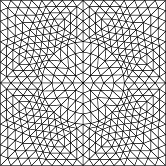
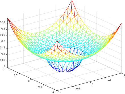
Fig. 1: Finite element mesh and solution for Example 5.1 with $\beta^{+}=10,\beta^{-}=1$: (a) Body-fitted mesh on the second level; (b) Finite element solution on the body-fitted mesh.

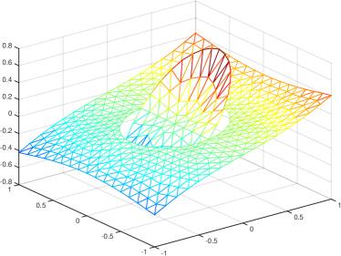
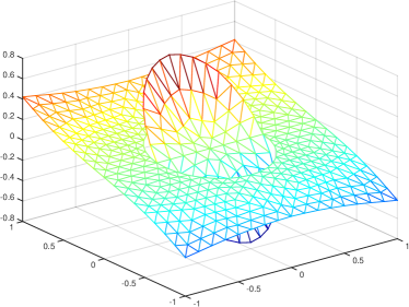
Fig. 2: Plot of recovered gradient for Example 5.1 with $\beta^{+}=10,\beta^{-}=1$: (a) $x$-component; (b) $y$-component.

Here we use five different levels of body-fitted meshes generated by Delaunay mesh generator. figure 1 plots the second level body-fitted mesh and figure 1 plots the finite element solution on such a mesh. figure 2 shows the recovered gradient.

Table 1: Numerical results for Example 5.1 with $\beta^{+}=10,\beta^{-}=1$.

Dof	$De$	order	$D^{i}e$	order	$D^{r}e$	order	$D^{p}e$	order
129	1.35e-01	–	1.63e-02	–	1.34e-01	–	2.44e-01	–
481	7.25e-02	0.48	5.00e-03	0.90	2.30e-02	1.34	1.80e-01	0.23
1857	3.69e-02	0.50	1.40e-03	0.94	6.82e-03	0.90	1.30e-01	0.24
7297	1.85e-02	0.50	3.76e-04	0.96	1.84e-03	0.96	9.24e-02	0.25
28929	9.29e-03	0.50	9.81e-05	0.97	4.78e-04	0.98	6.52e-02	0.25

Table 2: Numerical results for Example 5.1 with $\beta^{+}=1000,\beta^{-}=1$.

Dof	$De$	order	$D^{i}e$	order	$D^{r}e$	order	$D^{p}e$	order
129	1.25e-01	–	1.51e-02	–	1.47e-01	–	2.76e-01	–
481	6.76e-02	0.47	4.63e-03	0.90	2.29e-02	1.41	2.01e-01	0.24
1857	3.45e-02	0.50	1.29e-03	0.95	6.78e-03	0.90	1.45e-01	0.24
7297	1.73e-02	0.50	3.39e-04	0.98	1.83e-03	0.96	1.03e-01	0.25
28929	8.68e-03	0.50	8.70e-05	0.99	4.75e-04	0.98	7.24e-02	0.25

Table 3: Numerical results for Example 5.1 with $\beta^{+}=1000000,\beta^{-}=1$.

Dof	$De$	order	$D^{i}e$	order	$D^{r}e$	order	$D^{p}e$	order
129	1.25e-01	–	1.51e-02	–	1.47e-01	0.00	2.76e-01	–
481	6.76e-02	0.47	4.63e-03	0.90	2.29e-02	1.41	2.01e-01	0.24
1857	3.45e-02	0.50	1.29e-03	0.95	6.78e-03	0.90	1.45e-01	0.24
7297	1.73e-02	0.50	3.39e-04	0.98	1.83e-03	0.96	1.03e-01	0.25
28929	8.68e-03	0.50	8.70e-05	0.99	4.75e-04	0.98	7.25e-02	0.25

Table 4: Numerical results for Example 5.1 with $\beta^{+}=1,\beta^{-}=1000000$.

Dof	$De$	order	$D^{i}e$	order	$D^{r}e$	order	$D^{p}e$	order
129	5.27e-01	–	6.02e-02	–	1.84e-01	0.00	3.51e-01	–
481	2.64e-01	0.53	1.70e-02	0.96	3.06e-02	1.36	2.14e-01	0.38
1857	1.32e-01	0.51	4.66e-03	0.96	8.06e-03	0.99	1.48e-01	0.28
7297	6.60e-02	0.51	1.26e-03	0.96	2.10e-03	0.98	1.03e-01	0.26
28929	3.30e-02	0.50	3.37e-04	0.96	5.40e-04	0.98	7.25e-02	0.26

tables 1, 2, 3 and 4 show the numerical results for four typical different jump ratios: $\beta^{-}/\beta^{+}=1/10$ (moderate jump), $\beta^{-}/\beta^{+}=1/1000$ (large jump), $\beta^{-}/\beta^{+}=1/1000000$ (huge jump), and $\beta^{-}/\beta^{+}=1000000$ (huge jump). In all different cases, optimal $\mathcal{O}(h)$ convergence can be observed for $H^{1}$-semi error of finite element solution as given in theorem 2.1. Notice that in this example, $g=0$ and $\Gamma$ is arbitrary smooth. As discussed in 7, one can have the supercloseness of $\mathcal{O}(h^{2})$ as observed in Column 5 of tables 1, 2, 3 and 4. One also notices that, for the convergence rate of gradients, IPPR ($D^{r}e$) superconverges at the order of $\mathcal{O}(h^{2})$ while PPR ($D^{p}e$) converges suboptimally at the order of $\mathcal{O}(h^{0.5})$.

Example 5.2. In this example, we consider the flower-shape interface problem as studied in [31, 46]. The computational domain is $(-1,1)\times(-1,1)$. The interface curve $\Gamma$ in polar coordinate is given by

$$r=\frac{1}{2}+\frac{\sin(5\theta)}{7},$$

which contains both convex and concave parts. The diffusion coefficient is piecewise constant with $\beta^{-}=1$ and $\beta^{+}=10$. The right hand function $f$ in (2.1) is chosen to match the exact solution

$$u(z)=\left\{\begin{array}[]{ll}e^{(x^{2}+y^{2})},&\text{if }z\in\Omega^{+}\\ 0.1(x^{2}+y^{2})^{2}-0.01\ln(2\sqrt{x^{2}+y^{2}}),&\text{if }z\in\Omega^{+},\\ \end{array}\right.$$

and the jump conditions at interface (2.4)-(2.5) are also provided by the exact solution.

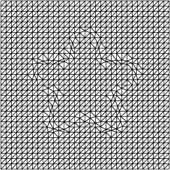
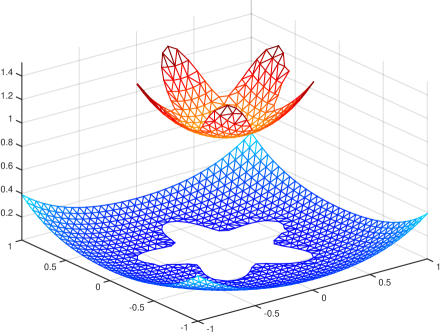
Fig. 3: Finite element mesh and solution for Example 5.2: (a) Body-fitted mesh on the first level; (b) Finite element solution on the body-fitted mesh.

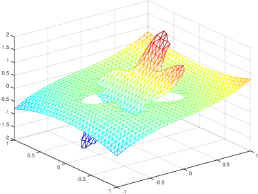
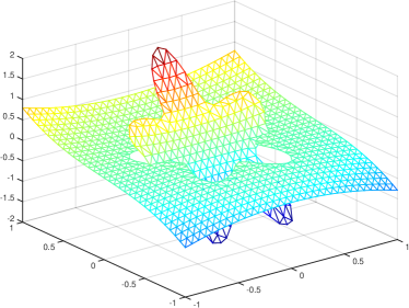
Fig. 4: Plot of recovered gradient for Example 5.2: (a) $x$-component; (b) $y$-component.

We use Börgers algorithm [5] to generate the body-fitted meshes, with the first level of mesh shown in figure 3 and the finite element solution in figure 3. figure 4 gives the plot of recovered gradient.

In table 5, one can see that $De$ decays at the rate of $\mathcal{O}(h)$, and $D^{i}e$ superconverges at the rate of $\mathcal{O}(h^{1.5})$ which is consistent with theorem 4.2. IPPR ($D^{r}e$) has an $\mathcal{O}(h^{1.5})$ superconvergence that agrees with theorem 4.3. However, no convergence is observed for standard PPR gradient recovery ($D^{p}e$) since the exact solution is only smooth on each subdomain.

Table 5: Convergence rate for Example 5.2.

Dof	$De$	order	$D^{i}e$	order	$D^{r}e$	order	$D^{p}e$	order
1089	7.25e-02	–	1.29e-02	–	1.15e-02	–	6.40e-01	–
4225	3.72e-02	0.49	4.67e-03	0.75	3.74e-03	0.83	6.35e-01	0.01
16641	1.87e-02	0.50	1.68e-03	0.74	1.19e-03	0.83	6.36e-01	-0.00
66049	9.42e-03	0.50	6.06e-04	0.74	3.75e-04	0.84	6.34e-01	0.00
263169	4.72e-03	0.50	2.18e-04	0.74	1.27e-04	0.78	6.34e-01	0.00
1050625	2.36e-03	0.50	7.69e-05	0.75	4.49e-05	0.75	6.33e-01	0.00

Example 5.3 This is the same example as used in [18]. We decompose the computational domain $\Omega=(0,1)\times(0,1)$ into two parts: $\Omega^{-}=\{z=(x,y)\in\Omega:x>0,y>0\}$ and $\Omega^{+}=\Omega\setminus\Omega^{-}$. The diffusion coefficient $\beta$ in (2.1) is chosen as

$$\beta(z)=\left\{\begin{array}[]{ccc}\beta^{-}&\text{if }z\in\Omega^{-},\\ 1&\text{if }z\in\Omega^{+},\end{array}\right.$$

with $\beta^{-}$ as a constant. When $f=0$ in (2.1), the exact solution $u$ in polar coordinate is given by

$$u(r,\theta)=\left\{\begin{array}[]{llc}r^{\mu}\cos(\mu(\theta-\pi/4))&\text{if }0\leq\theta\leq\pi/2,\\ r^{\mu}\nu\cos(\mu(\theta-5\pi/4))&\text{if }\pi/2\leq\theta\leq 2\pi,\\ \end{array}\right.$$

where

$$\mu=\frac{4}{\pi}\left(\sqrt{\frac{3+\beta^{-}}{1+3\beta^{-}}}\right)\quad\text{ and }\quad\nu=-\beta^{-}\frac{\sin(\mu\pi/4)}{\sin(3\mu\pi/4)}.$$

Note that $u\in H^{1+s}(\Omega^{\pm})$ for any $0<s<\mu$.

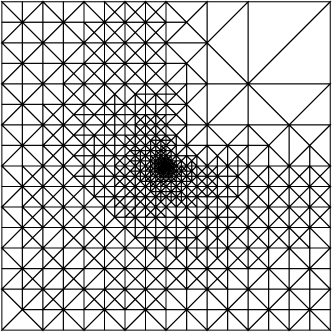
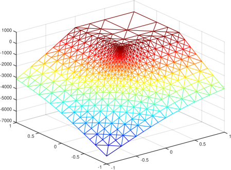
Fig. 5: Adaptive refined and solution of Example 5.3 with $\beta^{-}=10000$. (a) Adaptive refined mesh. (b). Finite element solution on adaptive refined mesh h.

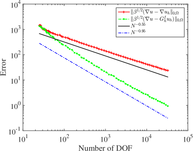
Fig. 6: Convergence rates for Example 5.3: (a) $\beta^{-}=1000$; (b) $\beta^{-}=10000$.

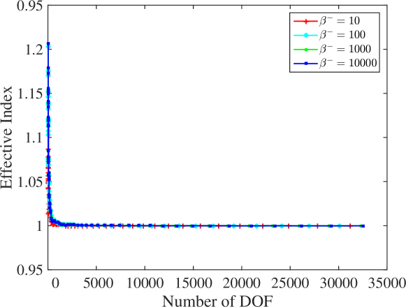
Fig. 7: Graph of effective index of Example 5.3

When $\beta^{-}>1$, there is a singularity at the origin. To obtain optimal convergence rate, we use adaptive finite element method based on the recovery-type a posteriori error estimator equation 4.18. The bulk marking strategy by [17] with $\theta=0.2$ is used in numerical computation. We start with a uniform initial mesh consisting of $32$ right triangles. Here, we consider the cases when $\beta^{-}=10,100,1000$, and $10000$. figure 5 plots an adaptive refined mesh and figure 5 shows the finite element solution when $\beta^{-}=10000$. It shows clearly that the refinement is concentrated on the singularity point.

figures 6 and 6 give the numerical convergence rates for $\beta^{-}=1000$ and $\beta^{-}=10000$ respectively. In both cases, optimal convergence of $\mathcal{O}(N^{-0.5})$ for energy error and superconvergence rate of $\mathcal{O}(N^{0.95})$ can be observed, which is consistent with theorem 4.7. We also plot the effective index

$$\kappa=\frac{\eta_{h}}{\|\beta^{1/2}(\nabla u-\nabla u_{h})\|_{0,\Omega}}$$

in figure 7. It shows the error indicator equation 4.18 is an asymptotically exact a posteriori error estimator for interface problem as in theorem 4.8

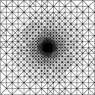
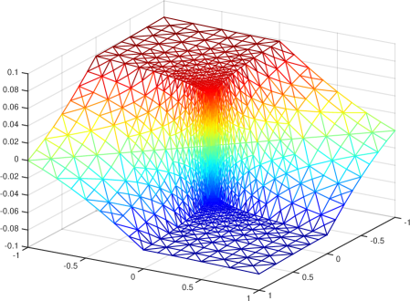
Fig. 8: Adaptive refined and solution of Example 5.3 with $\beta^{-}=10000$. (a) Adaptive refined mesh. (b). Finite element solution on adaptive refined mesh h.

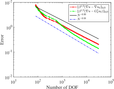
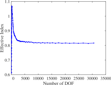
Fig. 9: Convergence rates for Example 5.3: (a) Errors; (b) Effective index.

Example 5.4. In the example, we consider the Kellogg problem which is the benchmark problem of adaptive finite element method for interface problem studied by, for example, [8, 12, 30, 22]. We choose the computational domain $\Omega=(0,1)\times(0,1)$, and consider equation 2.1 with $\beta(x)=R$ in the first and third quadrants and $\beta(x)=1$ in the second and fourth quadrants. When $f=0$ in equation 2.1, the exact solution $u$ in polar coordinates is given by $u(r,\theta)=r^{\epsilon}\mu(\theta)$ with

$$\mu(\theta)=\left\{\begin{array}[]{llc}\cos((\pi/2-\xi)\epsilon)\cdot\cos((\theta-\pi/2+\nu)\epsilon)&\text{if }0\leq\theta\leq\pi/2,\\ \cos(\nu\epsilon)\cdot\cos((\theta-\pi+\xi)\epsilon)&\text{if }\pi/2\leq\theta\leq\pi,\\ \cos(\xi\epsilon)\cdot\cos((\theta-\pi-\nu)\epsilon)&\text{if }\pi\leq\theta\leq 3\pi/2,\\ \cos((\pi/2-\nu)\epsilon)\cdot\cos((\theta-3\pi/2-\xi)\epsilon)&\text{if }3\pi/2\leq\theta\leq 2\pi,\end{array}\right.$$

with the constants $\epsilon,R,\xi$ and $\nu$ satisfying the nonlinear relations in [12, 22]. Here we choose

$$\epsilon=0.1,\quad\nu=\pi/4,\quad\xi=-14.9225565104455152,\quad R=161.4476387975881,$$

and then the exact solution $u\in H^{1+\epsilon}$ with a singularity at the origin.

We start with a uniform initial mesh consisting of $128$ right triangles and adopt bulk marking strategy by [17] with $\theta=0.2$. figure 8 plots one adaptive refined mesh and figure 8 plots its corresponding finite element solution. It clearly indicates that recovery type a posteriori error estimator equation 4.18 successfully captures the singularity without introducing any overrefinement. However, the recovery type a posteriori error estimator based on classical gradient recovery operators like SPR or PPR have the problem of overfinement as discussed in [8].

figure 9 shows the numerical errors. One can observe the optimal convergence rate $\mathcal{O}(N^{0.5})$ for energy error and $\mathcal{O}(N^{0.58})$ superconvergence rate for recovered energy error. figure 9 gives the history of effective index. Due to extreme low global regularity of exact solution, the recovery type a posteriori error estimator equation 4.18 is not asymptotically exact. However, it serves as a robust a posteriori error estimator for interface problem as illustrated in figure 8.

6 Conclusion

In this paper, we develop a novel gradient recovery method for elliptic interface problem based on body-fitted mesh. Specifically, we define an immersed gradient recovery operator, which overcomes the drawback that stand gradient recovery method fails to produce superconvergence results when solution is lack of regularity at interface. The superconvergence of this method is proved for both mildly unstructured mesh and adaptive mesh. Several two-dimensional numerical examples are given to confirm our theoretical results, and verify the robustness of the method served as a posteriori error estimator. As a continuous study, we plan to develop gradient recovery methods based on unfitted mesh for elliptic interface problem.

References

- [1] M. Ainsworth and J. T. Oden, A posteriori error estimation in finite element analysis, Pure and Applied Mathematics (New York), Wiley-Interscience [John Wiley & Sons], New York, 2000.
- [2] I. Babuška, The finite element method for elliptic equations with discontinuous coefficients, Computing (Arch. Elektron. Rechnen), 5 (1970), pp. 207–213.
- [3] I. Babuška and T. Strouboulis, The finite element method and its reliability, Numerical Mathematics and Scientific Computation, The Clarendon Press, Oxford University Press, New York, 2001.
- [4] C. Bernardi and R. Verfürth, Adaptive finite element methods for elliptic equations with non-smooth coefficients, Numer. Math., 85 (2000), pp. 579–608.
- [5] C. Börgers, A triangulation algorithm for fast elliptic solvers based on domain imbedding, SIAM J. Numer. Anal., 27 (1990), pp. 1187–1196.
- [6] J. H. Bramble and J. T. King, A finite element method for interface problems in domains with smooth boundaries and interfaces, Adv. Comput. Math., 6 (1996), pp. 109–138 (1997).
- [7] S. C. Brenner and L. R. Scott, The mathematical theory of finite element methods, vol. 15 of Texts in Applied Mathematics, Springer, New York, third ed., 2008.
- [8] Z. Cai and S. Zhang, Recovery-based error estimator for interface problems: conforming linear elements, SIAM J. Numer. Anal., 47 (2009), pp. 2132–2156.
- [9] Z. Cai and S. Zhang, Recovery-based error estimators for interface problems: mixed and nonconforming finite elements, SIAM J. Numer. Anal., 48 (2010), pp. 30–52.
- [10] C. Chen, Structure Theory of Superconvergence of Finite Elements (in Chinese), Hunan Science and Technique Press, Changsha, 2001.
- [11] L. Chen and J. Xu, A posteriori error estimator by post-processing, in Adaptive Computations: Theory and Algorithms, J. Xu and T. Tang, eds., Science Press, Beijing, 2007, pp. 34–67.
- [12] Z. Chen and S. Dai, On the efficiency of adaptive finite element methods for elliptic problems with discontinuous coefficients, SIAM J. Sci. Comput., 24 (2002), pp. 443–462 (electronic).
- [13] Z. Chen and J. Zou, Finite element methods and their convergence for elliptic and parabolic interface problems, Numer. Math., 79 (1998), pp. 175–202.
- [14] S.-H. Chou, An immersed linear finite element method with interface flux capturing recovery, Discrete Contin. Dyn. Syst. Ser. B, 17 (2012), pp. 2343–2357.
- [15] S.-H. Chou and C. ATTANAYAKE, Flux recovery and superconvergence of quadratic immersed interface finite elements, DEC 2015, arXiv:1512.04563 [math.NA].
- [16] P. G. Ciarlet, The finite element method for elliptic problems, vol. 40 of Classics in Applied Mathematics, Society for Industrial and Applied Mathematics (SIAM), Philadelphia, PA, 2002. Reprint of the 1978 original [North-Holland, Amsterdam; MR0520174 (58 #25001)].
- [17] W. Dörfler, A convergent adaptive algorithm for Poisson’s equation, SIAM J. Numer. Anal., 33 (1996), pp. 1106–1124.
- [18] S. Du, R. Lin, and Z. Zhang, A posteriori error analysis of multipoint flux mixed finite element methods for interface problems, Advances in Computational Mathematics, (2016), pp. 1–25.
- [19] L. C. Evans, Partial differential equations, vol. 19 of Graduate Studies in Mathematics, American Mathematical Society, Providence, RI, second ed., 2010.
- [20] S. Hou and X.-D. Liu, A numerical method for solving variable coefficient elliptic equation with interfaces, J. Comput. Phys., 202 (2005), pp. 411–445.
- [21] T. Y. Hou, X.-H. Wu, and Y. Zhang, Removing the cell resonance error in the multiscale finite element method via a Petrov-Galerkin formulation, Commun. Math. Sci., 2 (2004), pp. 185–205.
- [22] R. B. Kellogg, On the Poisson equation with intersecting interfaces, Applicable Anal., 4 (1974/75), pp. 101–129. Collection of articles dedicated to Nikolai Ivanovich Muskhelishvili.
- [23] M. Křížek, H.-G. Roos, and W. Chen, Two-sided bounds of the discretization error for finite elements, ESAIM Math. Model. Numer. Anal., 45 (2011), pp. 915–924.
- [24] R. J. LeVeque and Z. L. Li, The immersed interface method for elliptic equations with discontinuous coefficients and singular sources, SIAM J. Numer. Anal., 31 (1994), pp. 1019–1044.
- [25] Z. Li, The immersed interface method using a finite element formulation, Appl. Numer. Math., 27 (1998), pp. 253–267.
- [26] Z. Li and K. Ito, The immersed interface method, vol. 33 of Frontiers in Applied Mathematics, Society for Industrial and Applied Mathematics (SIAM), Philadelphia, PA, 2006. Numerical solutions of PDEs involving interfaces and irregular domains.
- [27] Z. Li, T. Lin, Y. Lin, and R. C. Rogers, An immersed finite element space and its approximation capability, Numer. Methods Partial Differential Equations, 20 (2004), pp. 338–367.
- [28] Z. Li, T. Lin, and X. Wu, New Cartesian grid methods for interface problems using the finite element formulation, Numer. Math., 96 (2003), pp. 61–98.
- [29] Q. Lin, H. Xie, and J. Xu, Lower bounds of the discretization error for piecewise polynomials, Math. Comp., 83 (2014), pp. 1–13.
- [30] P. Morin, R. H. Nochetto, and K. G. Siebert, Convergence of adaptive finite element methods, SIAM Rev., 44 (2002), pp. 631–658 (electronic) (2003). Revised reprint of “Data oscillation and convergence of adaptive FEM” [SIAM J. Numer. Anal. 38 (2000), no. 2, 466–488 (electronic); MR1770058 (2001g:65157)].
- [31] L. Mu, J. Wang, G. Wei, X. Ye, and S. Zhao, Weak Galerkin methods for second order elliptic interface problems, J. Comput. Phys., 250 (2013), pp. 106–125.
- [32] A. Naga and Z. Zhang, A posteriori error estimates based on the polynomial preserving recovery, SIAM J. Numer. Anal., 42 (2004), pp. 1780–1800 (electronic).
- [33] A. Naga and Z. Zhang, The polynomial-preserving recovery for higher order finite element methods in 2D and 3D, Discrete Contin. Dyn. Syst. Ser. B, 5 (2005), pp. 769–798.
- [34] S. Osher and R. Fedkiw, Level set methods and dynamic implicit surfaces, vol. 153 of Applied Mathematical Sciences, Springer-Verlag, New York, 2003.
- [35] C. S. Peskin, Numerical analysis of blood flow in the heart, J. Computational Phys., 25 (1977), pp. 220–252.
- [36] C. S. Peskin, The immersed boundary method, Acta Numer., 11 (2002), pp. 479–517.
- [37] J. A. Roĭtberg and Z. G. Šeftel\cprime, A theorem on homeomorphisms for elliptic systems and its applications, Mathematics of the USSR-Sbornik, 78 (3) (1969), pp. 439–465.
- [38] J. A. Sethian, Level set methods, vol. 3 of Cambridge Monographs on Applied and Computational Mathematics, Cambridge University Press, Cambridge, 1996. Evolving interfaces in geometry, fluid mechanics, computer vision, and materials science.
- [39] L. B. Wahlbin, Superconvergence in Galerkin finite element methods, vol. 1605 of Lecture Notes in Mathematics, Springer-Verlag, Berlin, 1995.
- [40] H. Wei, L. Chen, Y. Huang, and B. Zheng, Adaptive mesh refinement and superconvergence for two-dimensional interface problems, SIAM J. Sci. Comput., 36 (2014), pp. A1478–A1499.
- [41] H. Wu and Z. Zhang, Can we have superconvergent gradient recovery under adaptive meshes?, SIAM J. Numer. Anal., 45 (2007), pp. 1701–1722.
- [42] J. Xu, Error estimates of the finite element method for the 2nd order elliptic equations with discontinuous coefficients, J. Xiangtan Univ., 1 (1982), pp. 1–5.
- [43] J. Xu and Z. Zhang, Analysis of recovery type a posteriori error estimators for mildly structured grids, Math. Comp., 73 (2004), pp. 1139–1152 (electronic).
- [44] Z. Zhang and A. Naga, A new finite element gradient recovery method: superconvergence property, SIAM J. Sci. Comput., 26 (2005), pp. 1192–1213 (electronic).
- [45] X. Zheng and J. Lowengrub, An interface-fitted adaptive mesh method for elliptic problems and its application in free interface problems with surface tension, Adv. Comput. Math., (2016), pp. 1–33.
- [46] Y. C. Zhou and G. W. Wei, On the fictitious-domain and interpolation formulations of the matched interface and boundary (MIB) method, J. Comput. Phys., 219 (2006), pp. 228–246.
- [47] Q. Zhu and Q. Lin, Superconvergence Theory of the Finite Element Method (in Chinese), Hunan Science and Technique Press, Changsha, 1989.
- [48] O. C. Zienkiewicz and J. Z. Zhu, The superconvergent patch recovery and a posteriori error estimates. I. The recovery technique, Internat. J. Numer. Methods Engrg., 33 (1992), pp. 1331–1364.
- [49] O. C. Zienkiewicz and J. Z. Zhu, The superconvergent patch recovery and a posteriori error estimates. II. Error estimates and adaptivity, Internat. J. Numer. Methods Engrg., 33 (1992), pp. 1365–1382.