The Vlasov formalism for extended relativistic mean field models: the crust-core transition and the stellar matter equation of state

Abstract

The Vlasov formalism is extended to relativistic mean-field hadron models with non-linear terms up to fourth order and applied to the calculation of the crust-core transition density. The effect of the nonlinear $\omega\rho$ and $\sigma\rho$ coupling terms on the crust-core transition density and pressure, and on the macroscopic properties of some families of hadronic stars is investigated. For that purpose, six families of relativistic mean field models are considered. Within each family, the members differ in the symmetry energy behavior. For all the models, the dynamical spinodals are calculated, and the crust-core transition density and pressure, and the neutron star mass-radius relations are obtained. The effect on the star radius of the inclusion of a pasta calculation in the inner crust is discussed. The set of six models that best satisfy terrestrial and observational constraints predicts a radius of 13.6$\pm$0.3 km and a crust thickness of $1.36\pm 0.06$km for a 1.4 $M_{\odot}$ star.

I Introduction

The dynamical response of nuclear matter in the collisionless, low energy regime is adequately described within the Vlasov equation, a semi-classical approach that takes into account the correct particle statistics. It is a good approximation to the time-dependent Hartree-Fock equation at low energies Tang et al. (1981), and was used to study heavy-ion collisions at low-intermediate energies Jin et al. (1989); Ko and Li (1988, 1987); Li and Ko (1988). In Refs. Nielsen et al. (1991, 1993), the collective modes in cold and hot nuclear matter described with the Walecka model were successfully calculated within this formalism. An extension of the formalism was carried out including non-linear meson terms in the Lagrangian density Avancini et al. (2005); Providência et al. (2006a); Pais et al. (2009, 2010) or density-dependent meson couplings Santos et al. (2008). It has also been shown to be a good tool to estimate the crust-core transition in cold neutrino-free neutron stars Avancini et al. (2010, 2012). Similar calculations based on the Skyrme interaction had been developed previously Pethick et al. (1995). In Refs. Avancini et al. (2010, 2012), different calculations of the transition density at several temperatures and isospin asymmetries were compared, and it was found that the dynamical spinodal method predicts a lower limit for the crust-core density, and, that the larger the isospin asymmetry, the closer this value is to the Thomas Fermi estimate. For $\beta$-equilibrium matter, i.e., neutron star matter, both results are very similar.

Unified equations of state (EoS), that is, EoS that describe the neutron star, from its outer crust to the inner core within the same nuclear model, are generally not available. Consequently, the complete EoS is frequently built out of three different pieces, one for the outer crust, another for the inner crust, and one for the core, obtained from different models. Recently, it was shown in Fortin et al. (2016), that although star properties such as mass and radius do not depend on the outer crust EoS, the choice of the inner crust EoS and the matching of the inner crust EoS to the core EoS may be critical, and variations larger than 0.5 km have been obtained for the radius of a 1.4 $M_{\odot}$ star.

For the outer crust, three EoS are used in the literature: the Baym-Pethick-Sutherland (BPS) EoS Baym et al. (1971), the Haensel and Pichon (HP) EoS Haensel and Pichon (1994), or the Rüster et al (RHS) EoS Rüster et al. (2006). Essentially, the differences existing among them do not affect the mass-radius curves. This is not anymore true for matter above the neutron drip line. The inner crust of neutron stars may contain exotic geometrical structures termed nuclear pasta Ravenhall et al. (1983) at its upper boarder, just before the crust-core transition. Several methods have been used to compute these pasta phases: quantum Watanabe et al. (2009), semiclassical Horowitz et al. (2005); Schneider et al. (2016) or classical Dorso et al. (2012) Molecular Dynamics calculations, 3D Hartree-Fock calculations Newton and Stone (2009); Pais and Stone (2012) and Thomas-Fermi (TF) calculations Maruyama et al. (2005); Avancini and Bertolino (2015); Avancini et al. (2010, 2012); Okamoto et al. (2013). The authors of Pons et al. (2013) attribute to the existence of pasta phases a high impurity parameter corresponding to a large resistivity that causes a very fast magnetic field decay and explains the absence of isolated pulsars with periods above 12 s. In the present study, the complete stellar matter EoS will be constructed by taking (1) a standard EoS for the outer crust, such as BPS, HP or RHS, (2) an adequate inner crust EoS that matches the outer crust EoS at the neutron drip, and the core EoS at the crust-core transition, and (3) the core EoS. After having the complete EoS, star properties such as the mass and radius are determined from the integration of the TOV equations Tolman (1939); Oppenheimer and Volkoff (1939).

Laboratory measurements and first principle calculations put limits on the EoS that describe neutron stars. An example are the microscopic calculations based on nuclear interactions derived from chiral effective field theory Hebeler et al. (2013), or on realistic two- and three-nucleon interactions, using quantum Monte Carlo (MC) techniques Gandolfi et al. (2012). However, in these approaches there is a reasonable uncertainty associated with the three-body force, meaning that small differences between RMF models and MC results should not be enough to discard those models. Other constraints come from terrestrial experiments, like collective flow data in heavy-ion collisions Danielewicz et al. (2002) and the KaoS experiment Lynch et al. (2009), or the measurement of saturation density properties and properties of nuclei such as the binding energy and rms radii Tsang et al. (2012). Observational constraints also play a fundamental role. In 2010 and 2013, two very massive pulsars, PSR J1614-2230 Demorest et al. (2010) and PSR J0348+0432 Antoniadis et al. (2013), respectively, both close to $M\sim 2M_{\odot}$, were observed. An updated determination of the PSR J1614-2230 mass has reduced this value to 1.928$\pm 0.017M_{\odot}$ Fonseca et al. (2016). Radii are still not sufficiently constrained, but ESA missions such as the Advanced Telescope for High-energy Astrophysics (Athena+) Barret et al. (2013) and the Theia space mission will allow, amongst other things, to better constraint the $M/R$ relation of neutron stars.

Appropriate nuclear models should satisfy both kinds of constraints, observational and terrestrial. The NL3 Lalazissis et al. (1997) parametrization has been fitted to ground-state properties of both stable and unstable nuclei. It is able to predict 2$M_{\odot}$, but has a too large symmetry energy slope, and is too hard at high densities. Other nucleonic EOS that satisfy the $2M_{\odot}$ constraint have been discussed in the literature, see for instance Lattimer (2012); Weissenborn et al. (2012); Bonanno and Sedrakian (2012). However, some nucleonic models agree well with the phenomenology at low and intermediate densities, but fail to produce 2 $M_{\odot}$ stars because they predict a too soft EoS. Introducing adequate new non-linear terms in the Lagrangian density will change the density dependence of the EoS, so as to correct its behavior either by inducing a softening Horowitz and Piekarewicz (2001); Carriere et al. (2003); Sugahara and Toki (1994) or hardening Shen et al. (2011); Maslov et al. (2015) of the EoS. Experimental results at intermediate densities are essential to constrain these terms.

The transition pressure plays a very important role in the determination of the fraction of the star moment of inertia contained in the crust Link et al. (1999). The description of glitches considers that the inner crust is a reservoir of angular momentum, and, in Ref. Link et al. (1999), the authors have estimated that the observed glitches of Vela would be explained if 1.4% of the total momentum of inertia of the star resides in the crust. More recently, it was shown that crustal entrainement requires, in fact, a larger angular momentum reservoir in the crust Chamel (2013), associated to a fraction of the total momentum of inertia larger than the one the crust may contain. Possible solutions to solve this problem include the contribution of the core to the glitch mechanism Andersson et al. (2012), or the choice of an appropriate EoS that predicts a sufficiently large pressure at the crust-core transition Piekarewicz et al. (2014).

We will analyse the effect of the $\sigma\rho$ and $\omega\rho$ couplings on the crust-core transition density and pressure at zero temperature, starting from three different relativistic mean-field (RMF) models, TM1 Sugahara and Toki (1994), NL3 Lalazissis et al. (1997) and Z271 Horowitz and Piekarewicz (2001); Carriere et al. (2003). These three models will be designated head of the families of the models that we are going to construct, by adding the terms $\sigma\rho$ or $\omega\rho$ with different coupling strengths. Thus, in the following work, we are going to consider six different RMF families. While NL3 and TM1 have been fitted to the ground state properties of several nuclei, the symmetry energy slope these models predict at saturation density is too high. Z271 with the NL3 saturation properties has a softer EoS at large densities due to the inclusion of a fourth order term in $\omega$. The first two predict neutron stars with masses above the constraints set by the pulsars J1614-2230 and J0348+0432, while the third fails to satisfy these constraints. However, in Ref. Dutra et al. (2014), it has been shown that Z271$\omega\rho$5 and Z271$\omega\rho$6 were two of the few models that passed a set of 11 terrestrial constraints. We will consider several strengths of the couplings of the $\sigma\rho$ and $\omega\rho$ terms in order to generate a set of models that span the values of the symmetry energy and its slope at saturation as obtained in different experiments Tsang et al. (2012). It will be possible to identify existing correlations between the slope $L$ and the density and pressure transitions in a systematic way, since in each family the isoscalar properties are kept fixed and only the isovector properties change. We will then select, among the 6 families, the models that satisfy a set of well accepted saturation properties and constraints from microscopic calculations, and still produce a star with mass larger than $2M_{\odot}$. Since the Z271 family does not satisfy the last constraint, we will implement the mechanism proposed in Maslov et al. (2015), adding an extra non-linear $\sigma$ function that hardens the EoS above saturation.

One of the objectives of the work is to distinguish the effect of the terms of the form $\omega\rho$ and $\sigma\rho$ when modifying the density dependence of the symmetry energy. We will consider terms of the form $f_{i}^{2}\rho^{2}$, with $f_{i}=\omega$ or $\sigma$, as in Refs. Horowitz and Piekarewicz (2001); Carriere et al. (2003), which will affect the neutron skin thickness of nuclei but do not change some well established properties of nuclei, such as the binding energy and the charge radius. In Pais et al. (2016), where a non-linear $\sigma\rho$ term of the form $\sigma\rho^{2}$ was used, and a refitting of other parameters kept the binding energy and the charge radius unchanged, a non linear behavior of the transition density with $L$ was obtained, in contrast to previous studies Ducoin et al. (2010, 2011). We will also pay a special attention to the effect of these terms on the pressure at the crust-core transition, since this is a quantity that directly shows whether the glitch mechanism could be attributed solely to the crust.

In order to calculate the crust core transition properties, we extend the Vlasov formalism previously used to include all non-linear self-interaction and mixing terms involving the $\sigma,\,\omega$ and $\rho$ mesons up to fourth order. Taking the six families of models described above we will determine the crust-core transition density and pressure and will discuss possible implications of the different density dependence of the symmetry energy on the properties of neutron stars, especially the effects on the star radius.

In Section II, we present the formalism and derive the dispersion relation within the Vlasov method for the calculation of the dynamical spinodal with the non-linear $\sigma$, $\omega$, and $\rho$ mesons coupling terms. In Section III, the formalism is applied to the determination of the crust-core transition, and the construction of a consistent stellar matter EoS, and, finally, in Sec. IV, a few conclusions are drawn.

II Formalism

We use the relativistic non-linear Walecka model (NLWM) in the mean-field approximation, within the Vlasov formalism to study nuclear collective modes of asymmetric nuclear matter and $npe$ matter at zero temperature Nielsen et al. (1991, 1993). We will first review the Lagrangian density of the extended RMF model with all meson terms up to quartic order Furnstahl et al. (1996, 1997), and we will next present the Vlasov formalism to study the collective model of nuclear matter.

II.1 Extended RMF Lagrangian

We consider a system of baryons, with mass $M$, interacting with and through an isoscalar-scalar field $\phi$, with mass $m_{s}$, an isoscalar-vector field $V^{\mu}$, with mass $m_{v}$, and an isovector-vector field $\mathbf{b}^{\mu}$, with mass $m_{\rho}$. When describing $npe$ matter, we also include a system of electrons with mass $m_{e}$. Protons and electrons interact through the electromagnetic field $A^{\mu}$. The Lagrangian density reads:

$${\cal L}=\sum_{i=p,n}{\cal L}_{i}+{\cal L}_{e}+{\cal L}_{\sigma}+{\cal L}_{\omega}+{\cal L}_{\rho}+{\cal L}_{\sigma\omega\rho}+{\cal L}_{A}$$

where the nucleon Lagrangian reads

$${\cal L}_{i}=\bar{\psi}_{i}\left[\gamma_{\mu}iD^{\mu}-M^{*}\right]\psi_{i}\,,$$

with

$$iD^{\mu}=i\partial^{\mu}-g_{v}V^{\mu}-\frac{g_{\rho}}{2}{\boldsymbol{\tau}}\cdot\mathbf{b}^{\mu}-eA^{\mu}\frac{1+\tau_{3}}{2}\,,$$

$$M^{*}=M-g_{s}\phi\,,$$

and the electron Lagrangian is given by

$${\cal L}_{e}=\bar{\psi}_{e}\left[\gamma_{\mu}\left(i\partial^{\mu}+eA^{\mu}\right)-m_{e}\right]\psi_{e}.$$

The isoscalar part is associated with the scalar sigma ($\sigma$) field $\phi$, and the vector omega ($\omega$) field $V_{\mu}$, whereas the isospin dependence comes from the isovector-vector rho ($\rho$) field $b_{\mu}^{i}$ (where $\mu$ stands for the four dimensional space-time indices and $i$ the three-dimensional isospin direction index). The associated Lagrangians are:

$${\cal L}_{\sigma} = +\frac{1}{2}\left(\partial_{\mu}\phi\partial^{\mu}\phi-m_{s}^{2}\phi^{2}-\frac{1}{3}\kappa\phi^{3}-\frac{1}{12}\lambda\phi^{4}\right),$$

$${\cal L}_{\omega} = -\frac{1}{4}\Omega_{\mu\nu}\Omega^{\mu\nu}+\frac{1}{2}m_{v}^{2}V_{\mu}V^{\mu}+\frac{1}{4!}\xi g_{v}^{4}(V_{\mu}V^{\mu})^{2},$$

$${\cal L}_{\rho} = -\frac{1}{4}\mathbf{B}_{\mu\nu}\cdot\mathbf{B}^{\mu\nu}+\frac{1}{2}m_{\rho}^{2}\mathbf{b}_{\mu}\cdot\mathbf{b}^{\mu},$$

$${\cal L}_{A} = -\frac{1}{4}F_{\mu\nu}F^{\mu\nu},$$ (1)

where $\Omega_{\mu\nu}=\partial_{\mu}V_{\nu}-\partial_{\nu}V_{\mu},\quad\mathbf{B}_{\mu\nu}=\partial_{\mu}\mathbf{b}_{\nu}-\partial_{\nu}\mathbf{b}_{\mu}-g_{\rho}(\mathbf{b}_{\mu}\times\mathbf{b}_{\nu})$ and $F_{\mu\nu}=\partial_{\mu}A_{\nu}-\partial_{\nu}A_{\mu}$. We supplement the meson Lagrangian with all the non-linear terms that mix the $\sigma,\omega$, and $\mathbf{\rho}$ mesons up to quartic order Furnstahl et al. (1996, 1997); Sulaksono and Kasmudin (2009); Agrawal (2010),

$${\cal L_{\sigma\omega\rho}} = \Lambda_{3\sigma}g_{s}g_{v}^{2}\phi V_{\mu}V^{\mu}+\Lambda_{2\sigma}g_{s}^{2}g_{v}^{2}\phi^{2}V_{\mu}V^{\mu}$$ (2)

$$+ \Lambda_{1\sigma}g_{s}g_{\rho}^{2}\phi\mathbf{b}_{\mu}\cdot\mathbf{b}^{\mu}+\Lambda_{\sigma}g_{s}^{2}g_{\rho}^{2}\phi^{2}\mathbf{b}_{\mu}\cdot\mathbf{b}^{\mu}$$

$$+ \Lambda_{\omega}g_{v}^{2}g_{\rho}^{2}\mathbf{b}_{\mu}\cdot\mathbf{b}^{\mu}\,V_{\mu}V^{\mu}.$$

An adequate choice of the parameters of the model will allow to build parametrizations compatible with both laboratory measurements and astrophysical observations Sulaksono and Kasmudin (2009); Agrawal (2010). The model comprises the following parameters: three coupling constants, $g_{s}$, $g_{v}$, and $g_{\rho}$, of the mesons to the nucleons, the bare nucleon mass, $M$, the electron mass, $m_{e}$, the masses of the mesons, the electromagnetic coupling constant, $e=\sqrt{4\pi/137}$, the self-interacting coupling constants, $\kappa$, $\lambda$, and $\xi$, and the mixing self-interacting coupling constants, $\Lambda_{\omega},\Lambda_{\sigma},\Lambda_{i\sigma},i=1,2,3$. In this Lagrangian density, $\boldsymbol{\tau}$ are the Pauli matrices.

Table 1: Symmetric nuclear matter properties at saturation density, $\rho_{0}$, for the $\sigma\rho$ models. For TM1, the binding energy per nucleon, $E/A$, is -16.26 MeV, the incompressibility coefficient, $K$, is 280 MeV, and the nuclear saturation density is 0.145 fm^-3. For NL3 and Z271, these values are, respectively, -16.24 MeV, 270/269 MeV, and 0.148 fm^-3. $\rho_{t}$ and $P_{t}$ are the crust-core transition density and pressure, respectively, for $\beta-$equilibrium $pne$ matter, at $T=0$ MeV. $P_{N}$ is the pressure for neutron matter at $\rho=\rho_{0}$. The values of the total binding energy per particle ($B/A$), charge radii ($r_{c}$), neutron radii ($r_{n}$) and $\Delta r_{\rm np}$, for ²⁰⁸Pb, are also shown.

Model		$\Lambda_{\sigma}$		$E_{sym}$		$L$		$K_{sym}$		$K_{\tau}$		$\rho_{t}$		$P_{t}$		$P_{N}$		$B/A$		$r_{c}$		$r_{n}$		$\Delta r_{\rm np}$
				(MeV)		(MeV)		(MeV)		(MeV)		(fm-3)		(MeV/fm3)		(MeV/fm3)		(MeV)		(fm)		(fm)		(fm)
NL3		0		37.34		118		101		-696		0.055		0.258		5.978		-7.878		5.518		5.740		0.280
$\sigma\rho$1		0.004		35.85		99		4		-666		0.058		0.303		5.108		-7.891		5.519		5.723		0.262
$\sigma\rho$2		0.0072		34.88		88		-29		-620		0.063		0.365		4.546		-7.897		5.521		5.711		0.249
$\sigma\rho$3		0.011		33.85		76		-38		-553		0.069		0.408		4.004		-7.903		5.523		5.698		0.233
$\sigma\rho$4		0.0145		33		68		-28		-487		0.074		0.468		3.60		-7.908		5.526		5.686		0.218
$\sigma\rho$5		0.018		32.25		61		-6		-421		0.078		0.454		3.282		-7.911		5.530		5.675		0.203
$\sigma\rho$6		0.022		31.47		55		24		-348		0.081		0.382		2.991		-7.913		5.535		5.662		0.185
TM1		0		36.84		111		34		-517		0.060		0.328		5.479		-7.877		5.541		5.753		0.270
$\sigma\rho$1		0.004		34.99		94		-29		-499		0.064		0.360		4.724		-7.905		5.544		5.737		0.251
$\sigma\rho$2		0.0073		34.22		85		-56		-478		0.068		0.407		4.268		-7.910		5.545		5.727		0.239
$\sigma\rho$3		0.011		33.42		76		-67		-443		0.072		0.447		3.829		-7.915		5.548		5.716		0.226
$\sigma\rho$4		0.0146		32.72		68		-64		-403		0.076		0.458		3.469		-7.918		5.551		5.706		0.213
$\sigma\rho$5		0.019		31.93		60		-50		-350		0.079		0.427		3.104		-7.922		5.555		5.694		0.197
$\sigma\rho$6		0.022		31.43		56		-35		-313		0.080		0.379		2.896		-7.923		5.558		5.686		0.186
Z271		0		35.81		99		-16		-340		0.068		0.405		4.952		-7.777		5.519		5.702		0.241
$\sigma\rho$1		0.01		34.87		87		-65		-350		0.072		0.448		4.370		-7.784		5.521		5.691		0.229
$\sigma\rho$2		0.02		34.00		77		-92		-344		0.076		0.474		3.850		-7.791		5.522		5.680		0.216
$\sigma\rho$3		0.03		33.21		68		-104		-327		0.079		0.477		3.399		-7.797		5.524		5.670		0.203
$\sigma\rho$4		0.04		32.47		60		-106		-304		0.081		0.451		3.015		-7.802		5.527		5.659		0.191
$\sigma\rho$5		0.05		31.79		53		-100		-276		0.083		0.398		2.691		-7.806		5.530		5.649		0.177
$\sigma\rho$6		0.06		31.15		48		-88		-245		0.085		0.323		2.418		-7.810		5.533		5.639		0.164

Table 2: The same as in Table 1 for the $\omega\rho$ models.

Model		$\Lambda_{\omega}$		$E_{sym}$		$L$		$K_{sym}$		$K_{\tau}$		$\rho_{t}$		$P_{t}$		$P_{N}$		$B/A$		$r_{c}$		$r_{n}$		$\Delta r_{\rm np}$
				(MeV)		(MeV)		(MeV)		(MeV)		(fm-3)		(MeV/fm3)		(MeV/fm3)		(MeV)		(fm)		(fm)		(fm)
NL3		0		37.34		118		100		-696		0.055		0.258		5.978		-7.878		5.518		5.740		0.280
$\omega\rho$1		0.005		36.01		101		1		-680		0.057		0.291		5.146		-7.891		5.518		5.725		0.265
$\omega\rho$2		0.01		34.94		88		-46		-636		0.062		0.355		4.511		-7.899		5.519		5.712		0.251
$\omega\rho$3		0.015		33.98		77		-60		-578		0.068		0.437		3.998		-7.906		5.521		5.700		0.237
$\omega\rho$4		0.02		33.12		68		-53		-512		0.074		0.503		3.573		-7.912		5.524		5.688		0.223
$\omega\rho$5		0.025		32.36		61		-34		-445		0.080		0.533		3.213		-7.917		5.526		5.677		0.209
$\omega\rho$6		0.03		31.66		55		-8		-380		0.084		0.516		2.906		-7.921		5.530		5.667		0.195
TM1		0		36.84		111		33		-517		0.060		0.328		5.479		-7.877		5.541		5.753		0.270
$\omega\rho$1		0.005		35.12		95		-34		-511		0.063		0.350		4.760		-7.886		5.542		5.741		0.257
$\omega\rho$2		0.01		34.29		85		-73		-496		0.066		0.397		4.265		-7.872		5.542		5.733		0.249
$\omega\rho$3		0.015		33.54		76		-91		-468		0.071		0.455		3.845		-7.857		5.543		5.724		0.239
$\omega\rho$4		0.02		32.84		68		-94		-432		0.075		0.495		3.484		-7.828		5.545		5.715		0.228
$\omega\rho$5		0.025		32.20		61		-86		-392		0.079		0.510		3.167		- 7.817		5.548		5.703		0.213
$\omega\rho$6		0.03		31.61		56		-72		-350		0.082		0.497		2.885		-7.791		5.552		5.689		0.195
Z271		0		35.81		99		-16		-340		0.068		0.405		4.952		-7.777		5.519		5.702		0.241
$\omega\rho$1		0.01		35.25		91		-66		-364		0.071		0.436		4.574		-7.783		5.519		5.696		0.234
$\omega\rho$2		0.02		34.72		83		-104		-379		0.072		0.454		4.245		-7.788		5.519		5.689		0.228
$\omega\rho$3		0.025		34.46		80		-120		-383		0.073		0.473		4.095		-7.791		5.520		5.686		0.225
$\omega\rho$4		0.03		34.21		77		-133		-386		0.074		0.483		3.953		-7.793		5.520		5.683		0.222
$\omega\rho$5		0.035		33.97		74		-145		-388		0.075		0.498		3.818		-7.796		5.520		5.680		0.218
$\omega\rho$6		0.04		33.73		71		-154		-387		0.076		0.509		3.690		-7.798		5.520		5.677		0.215
$\omega\rho$7		0.05		33.27		65		-168		-383		0.079		0.533		3.451		-7.803		5.520		5.671		0.209
$\omega\rho$8		0.06		32.83		60		-178		-376		0.081		0.552		3.230		-7.807		5.521		5.665		0.203

II.2 The Vlasov formalism

In the sequel we use the formalism developed in Refs. Nielsen et al. (1991, 1993), where the collective modes in cold nuclear matter were determined within the Vlasov formalism, based on the Walecka model Walecka (1974). In the present section, we extend the Vlasov formalism and include all meson terms up to quartic order. We will use, whenever possible, the notation introduced in Nielsen et al. (1991, 1993).

The time evolution of the distribution functions, $f_{i}$, is described by the Vlasov equation

$$\frac{\partial f_{i}}{\partial t}+\{f_{i},h_{i}\}=0,\qquad\;i=p,\,n,\,e,$$ (3)

where $\{,\}$ denotes the Poisson brackets. The Vlasov equation expresses the conservation of the number of particles in phase space, and is, therefore, covariant.

The state that minimizes the energy of asymmetric nuclear matter is characterized by the Fermi momenta $P_{Fi},i=p,n$, $P_{Fe}=P_{Fp}$, and is described by the equilibrium distribution function at zero temperature

$$f_{0}({\boldsymbol{r}},{\boldsymbol{p}})=\mbox{diag}[\Theta(P_{Fp}^{2}-p^{2}),\Theta(P_{Fn}^{2}-p^{2}),\Theta(P_{Fe}^{2}-p^{2})]$$ (4)

and by the constant mesonic fields, that obey the following equations

$$m_{s}^{2}\phi_{0} + \frac{\kappa}{2}\phi_{0}^{2}+\frac{\lambda}{6}\phi_{0}^{3}-2\Lambda_{\sigma}g_{\sigma}^{2}g_{\rho}^{2}\phi_{0}b_{0}^{(0)2}-\Lambda_{1\sigma}g_{\sigma}g_{\rho}^{2}b_{0}^{(0)2}-2\Lambda_{2\sigma}g_{\sigma}^{2}g_{v}^{2}\phi_{0}V_{0}^{(0)2}-\Lambda_{3\sigma}g_{\sigma}g_{v}^{2}V_{0}^{(0)2}=g_{s}\rho_{s}^{(0)},\,\,\,$$

$$m_{v}^{2}\,V_{0}^{(0)} + \frac{1}{6}\xi g_{v}^{4}V_{0}^{(0)\,3}+2\Lambda_{\omega}g_{v}^{2}g_{\rho}^{2}V_{0}^{(0)}b_{0}^{(0)\,2}+2\Lambda_{2\sigma}g_{v}^{2}g_{\sigma}^{2}V_{0}^{(0)}\phi_{0}^{2}+2\Lambda_{3\sigma}g_{v}^{2}g_{\sigma}V_{0}^{(0)}\phi_{0}=g_{v}j_{0}^{(0)},\,\,\,$$

$$m_{\rho}^{2}\,b_{0}^{(0)} + 2\Lambda_{\omega}g_{\rho}^{2}g_{v}^{2}V_{0}^{(0)\,2}b_{0}^{(0)}+2\Lambda_{\sigma}g_{\rho}^{2}g_{\sigma}^{2}\phi_{0}^{2}b_{0}^{(0)}+2\Lambda_{1\sigma}g_{\rho}^{2}g_{\sigma}\phi_{0}b_{0}^{(0)}=\frac{g_{\rho}}{2}j_{3,0}^{(0)},\,\,\,$$

$$V^{(0)}_{i} = b_{i}^{(0)}=A_{0}^{(0)}=A_{i}^{(0)}=0,\,\,$$ (5)

where $\rho_{s}^{(0)},\,\,j_{0}^{(0)},\,\,j_{3,0}^{(0)}$ are, respectively, the equilibrium scalar density, the nuclear density, and the isospin density.

Collective modes correspond to small oscillations around the equilibrium state. The linearized equations of motion describe these small oscillations and the collective modes are the solutions of those equations. To construct them, let us define:

$$f_{i} = f_{0i}^{(0)}+\delta f_{i},$$

$$\phi\, = \,\phi_{0}+\delta\phi,$$

$$V_{0}\, = \,V_{0}^{(0)}+\delta V_{0},\quad V_{i}\,=\,\delta V_{i},$$

$$b_{0}\, = \,b_{0}^{(0)}+\delta b_{0},\quad b_{i}\,=\,\delta b_{i},$$

$$A_{0}\, = \,\delta A_{0},\quad A_{i}\,=\,\delta A_{i}.$$

As in Nielsen et al. (1991, 1993); Avancini et al. (2005, 2004), we express the fluctuations of the distribution functions in terms of the generating functions:

$$S({\mathbf{r}},{\mathbf{p}},t)=\mbox{diag}\left(S_{p},\,S_{n},\,S_{e}\right),$$

such that

$$\delta f_{i}=\{S_{i},f_{0i}\}=-\{S_{i},p^{2}\}\delta(P_{Fi}^{2}-p^{2}).$$

The linearized Vlasov equations for $\delta f_{i}$,

$$\frac{d\delta f_{i}}{dt}+\{\delta f_{i},h_{0i}\}+\{f_{0i},\delta h_{i}\}=0$$

are equivalent to the following time-evolution equations:

$$\frac{\partial S_{i}}{\partial t}+\{S_{i},h_{0i}\}=\delta h_{i} = -g_{s}\,\frac{M^{*}}{\epsilon_{0}}\delta\phi-\frac{{\bf p}\cdot\delta\boldsymbol{\cal V}_{i}}{\epsilon_{0}}+\delta{\cal V}_{0i},\,\,$$

$$i = p,n$$ (6)

$$\frac{\partial S_{e}}{\partial t}+\{S_{e},h_{0e}\}=\delta h_{e}=-e\left[\delta{A}_{0}-\frac{{\bf p}\cdot\delta{\mathbf{A}}}{\epsilon_{0e}}\right],$$ (7)

where

$$\delta{\cal V}_{0i} = g_{v}\delta V_{0}+\tau_{i}\frac{g_{\rho}}{2}\,\delta b_{0}+e\,\frac{1+\tau_{i}}{2}\,\delta A_{0},$$

$$\delta\boldsymbol{\cal V}_{i} = g_{v}\delta{\mathbf{V}}+\tau_{i}\frac{g_{\rho}}{2}\,\delta{\mathbf{b}}+e\,\frac{1+\tau_{i}}{2}\,\delta{\mathbf{A}}$$

$$h_{0i} = \epsilon_{0}+{\cal V}^{(0)}_{0i}\,=\sqrt{p^{2}+M^{*2}}+{\cal V}^{(0)}_{0i}$$

$$h_{0e} = \epsilon_{0e}=\sqrt{p^{2}+m^{2}_{e}}.$$

which has only to be satisfied for $p=P_{Fi}$.

The longitudinal modes, with wave vector ${\bf k}$ and frequency $\omega$, are described by the ansatz

$$\left(\begin{array}[]{c}S_{j}({\bf r},{\bf p},t)\\ \delta\phi\\ \delta\zeta_{0}\\ \delta\zeta_{i}\end{array}\right)=\left(\begin{array}[]{c}{\cal S}_{\omega}^{j}({\rm cos}\theta)\\ \delta\phi_{\omega}\\ \delta\zeta_{\omega}^{0}\\ \delta\zeta_{\omega}^{i}\end{array}\right){\rm e}^{i(\omega t-{\bf k}\cdot{\bf r})}\;,$$ (8)

where $j=p,\,n,\,e$, $\zeta=V,\,b,\,A$ represent the vector-meson fields, and $\theta$ is the angle between ${\bf p}$ and ${\bf k}$. The wave vector of the excitation mode, ${\bf k}$, is identified with the momentum transferred to the system, that gives rise to the excitation.

For the longitudinal modes, we get $\delta V_{\omega}^{x}=\delta V_{\omega}^{y}=0\,$, $\delta b_{\omega}^{x}=\delta b_{\omega}^{y}=0\,$ and $\delta A_{\omega}^{x}=\delta A_{\omega}^{y}=0\,$. Calling $\delta V_{\omega}^{z}=\delta V_{\omega}$, $\delta b_{\omega}^{z}=\delta b_{\omega}$ and $\delta A_{\omega}^{z}=\delta A_{\omega}$, we will have for the fields $\delta{\cal V}_{i,z}=\delta{\cal V}_{\omega}^{i}{\rm e}^{i(\omega t-{\bf k}\cdot{\bf r})}$ and $\delta{\cal V}_{0i}=\delta{\cal V}_{\omega}^{0i}{\rm e}^{i(\omega t-{\bf k}\cdot{\bf r})}.$ Replacing the ansatz (8) in Eqs. (II.2) and (7), we get

$$i\left(\omega-\omega_{0i}x\right){\cal S}_{\omega}^{i} = -g_{s}\frac{M^{*}}{\epsilon_{Fi}}\delta\phi_{\omega}-V_{Fi}x\delta{\cal V}_{\omega}^{i}$$ (9)

$$i\left(\omega-\omega_{0e}x\right){\cal S}_{\omega}^{e} = -e\delta{A}_{\omega}^{0}+eV_{Fe}x\delta{A}_{\omega},$$ (10)

$$\left(\omega^{2}-k^{2}-m^{2}_{s,eff}\right)\delta\phi_{\omega} = -\chi_{1}\delta b_{\omega}^{0}-\chi_{2}\delta V_{\omega}^{0}-\frac{2ig_{s}M^{*}}{(2\pi^{2})}\sum_{i=p,n}P_{Fi}\omega_{0i}\int_{-1}^{1}xS_{\omega}^{i}(x)dx$$ (11)

$$\left(\omega^{2}-k^{2}-m_{v,eff}^{2}\right)\delta V_{\omega}^{0} = \chi_{v}\delta b_{\omega}^{0}+\chi_{2}\delta\phi_{\omega}-\frac{2ig_{v}}{(2\pi^{2})}\sum_{i=p,n}\omega_{0i}P_{Fi}\epsilon_{Fi}\int_{-1}^{1}xS_{\omega}^{i}(x)dx,$$ (12)

$$\left(\omega^{2}-k^{2}-m_{\rho,eff}^{2}\right)\delta b_{\omega}^{0} = \chi_{v}\delta V_{\omega}^{0}+\chi_{1}\delta\phi_{\omega}-\frac{ig_{\rho}}{(2\pi^{2})}\sum_{i=p,n}\tau_{i}\omega_{0i}P_{Fi}\epsilon_{Fi}\int_{-1}^{1}xS_{\omega}^{i}(x)dx,$$ (13)

$$\left(\omega^{2}-k^{2}\right)\delta A_{\omega}^{0} = -\frac{2ei}{(2\pi^{2})}\sum_{i=p,e}\omega_{0i}P_{Fi}\epsilon_{Fi}\int_{-1}^{1}x(S_{\omega}^{p}(x)-S_{\omega}^{e}(x))dx,$$ (14)

with $x=\cos\theta$, $i=p,n$, $\omega_{0j}=kV_{Fj}=kP_{Fj}/\epsilon_{Fj}$, $j=p,n,e$, $\chi_{v}=4\Lambda_{\omega}g_{v}^{2}g_{\rho}^{2}V_{0}^{(0)}b_{0}^{(0)}$, $\chi_{1}=4\Lambda_{\sigma}g_{\sigma}^{2}g_{\rho}^{2}\phi_{0}b_{0}^{(0)}+2\Lambda_{1\sigma}g_{\sigma}g_{\rho}^{2}b_{0}^{(0)}$, $\chi_{2}=4\Lambda_{2\sigma}g_{\sigma}^{2}g_{v}^{2}\phi_{0}V_{0}^{(0)}+2\Lambda_{3\sigma}g_{\sigma}g_{v}^{2}V_{0}^{(0)}$, and

$$m_{s,eff}^{2} = m_{s}^{2}+\kappa\phi_{0}+\lambda/2\phi_{0}^{2}-2\Lambda_{\sigma}g_{\sigma}^{2}g_{\rho}^{2}b_{0}^{(0)2}-2\Lambda_{2\sigma}g_{\sigma}^{2}g_{v}^{2}V_{0}^{(0)2}+g_{s}^{2}\frac{d\rho_{s}^{0}}{dM^{*}}$$

$$m_{v,eff}^{2} = m_{v}^{2}+\frac{1}{2}g_{v}^{4}\xi V_{0}^{(0)2}+2\Lambda_{\omega}g_{v}^{2}g_{\rho}^{2}b_{0}^{(0)2}+2\Lambda_{2\sigma}g_{\sigma}^{2}g_{v}^{2}\phi_{0}^{2}+2\Lambda_{3\sigma}g_{\sigma}g_{v}^{2}\phi_{0}$$

$$m_{\rho,eff}^{2} = m_{\rho}^{2}+2\Lambda_{\omega}g_{\rho}^{2}g_{v}^{2}V_{0}^{(0)2}+2\Lambda_{\sigma}g_{\sigma}^{2}g_{\rho}^{2}\phi_{0}^{2}+2\Lambda_{1\sigma}g_{\sigma}g_{\rho}^{2}\phi_{0}$$ (15)

and from the continuity equation for the density currents, we get for the components of the vector fields

$$k\delta V_{\omega} = \omega\frac{B_{v}}{B_{v_{1}}}\delta V_{\omega}^{0}-\frac{\omega}{B_{v_{1}}}\left(\chi_{v}\delta b_{\omega}^{0}+\chi_{2}\delta\phi_{\omega}\right),$$ (16)

$$k\delta b_{\omega} = \omega\delta b_{\omega}^{0}-\frac{\omega}{B_{\rho}}\left(\chi_{v}\delta V_{\omega}^{0}+\chi_{1}\delta\phi_{\omega}\right),$$ (17)

$$k\delta A_{\omega} = \omega\delta A_{\omega}^{0}\,.$$ (18)

with $B_{v}=\omega^{2}-k^{2}-m_{v,eff}^{2}$, $B_{v_{1}}=\omega^{2}-k^{2}-m_{v,eff,1}^{2}$, $B_{\rho}=\omega^{2}-k^{2}-m_{\rho,eff}^{2}$, and $m_{v,eff,1}^{2}=m_{v}^{2}+\frac{1}{6}g_{v}^{4}\xi V_{0}^{(0)2}+2\Lambda_{\omega}g_{v}^{2}g_{\rho}^{2}b_{0}^{(0)2}+2\Lambda_{2\sigma}g_{\sigma}^{2}g_{v}^{2}\phi_{0}^{2}+2\Lambda_{3\sigma}g_{\sigma}g_{v}^{2}\phi_{0}$.

The solutions of Eqs. (9)-(14) form a complete set of eigenmodes that may be used to construct a general solution for an arbitrary longitudinal perturbation. Substituting the set of equations (11)-(14) into (9) and (10), we get a set of equations for the unknowns ${\cal S}_{\omega}^{i}$, which lead to the following matrix equation

$$\left(\begin{array}[]{ccc}1+F^{pp}L_{p}&F^{pn}L_{p}&C_{A}^{pe}L_{p}\\ F^{np}L_{n}&1+F^{nn}L_{n}&0\\ C_{A}^{ep}L_{e}&0&1-C_{A}^{ee}L_{e}\\ \end{array}\right)\left(\begin{array}[]{c}A_{\omega p}\\ A_{\omega n}\\ A_{\omega e}\end{array}\right)=0.$$ (19)

with $A_{\omega i}=\int_{-1}^{1}xS_{\omega i}(x)dx$, $L_{i}=L(s_{i})=2-s_{i}\ln((s_{i}+1)/(s_{i}-1))$, where $s_{i}=\omega/\omega_{0i}$, and $F^{ij}=C_{s}^{ij}-C_{v}^{ij}-C_{\rho}^{ij}-C_{A}^{ij}\delta_{ip}\delta_{ij}$, and

$$C_{A}^{ij}=-\frac{e^{2}}{2\pi^{2}}\frac{1}{k^{2}}\frac{P_{F}^{j2}}{V_{F}^{i}}$$

The coefficients $C_{s}^{ij},C_{v}^{ij}$ and $C_{\rho}^{ij}$ are given by:

$$C_{s}^{ij} = \left(1-\frac{\omega^{2}}{k^{2}}\left(\frac{g_{v}\chi_{2}}{B_{v_{1}}}+\frac{g_{\rho}\tau_{i}\chi_{1}}{2B_{\rho}}\right)\right)\frac{g_{\sigma}M^{*}}{2\pi^{2}P_{F_{i}}}\left(f_{\sigma}^{\sigma}g_{\sigma}M^{*}P_{F_{j}}V_{F_{j}}+f_{b}^{\sigma}\frac{g_{\rho}}{2}\tau_{j}P_{F_{j}}^{2}+f_{\omega}^{\sigma}g_{v}P_{F_{j}}^{2}\right)$$ (20)

$$C_{v}^{ij} = \left(1-\frac{\omega^{2}}{k^{2}}\left(\frac{B_{v}}{B_{v_{1}}}-\frac{g_{\rho}\tau_{i}\chi_{v}}{2g_{v}B_{\rho}}\right)\right)\frac{g_{v}}{2\pi^{2}V_{F_{i}}}\left(f_{\sigma}^{\omega}g_{\sigma}M^{*}P_{F_{j}}V_{F_{j}}+f_{b}^{\omega}\frac{g_{\rho}}{2}\tau_{j}P_{F_{j}}^{2}+f_{\omega}^{\omega}g_{v}P_{F_{j}}^{2}\right)$$ (21)

$$C_{\rho}^{ij} = \left(1-\frac{\omega^{2}}{k^{2}}\left(1-\frac{2g_{v}\chi_{v}}{g_{\rho}\tau_{i}B_{v_{1}}}\right)\right)\frac{g_{\rho}\tau_{i}}{4\pi^{2}V_{F_{i}}}\left(f_{\sigma}^{b}g_{\sigma}M^{*}P_{F_{j}}V_{F_{j}}+f_{b}^{b}\frac{g_{\rho}}{2}\tau_{j}P_{F_{j}}^{2}+f_{\omega}^{b}g_{v}P_{F_{j}}^{2}\right)$$ (22)

The coefficients $f_{i}^{j}$ read:

$$f_{\sigma}^{\sigma} = \frac{1}{S}\,,f_{b}^{\sigma}=-f_{\sigma}^{\sigma}\left(\frac{\chi_{1}\chi_{v}^{2}}{B_{\rho}D_{v}}+\frac{\chi_{1}}{B_{\rho}}+\frac{\chi_{2}\chi_{v}}{D_{v}}\right)\,,f_{\omega}^{\sigma}=-f_{\sigma}^{\sigma}\left(\frac{\chi_{2}\chi_{v}^{2}}{B_{v}D_{v}}+\frac{\chi_{2}}{B_{v}}+\frac{\chi_{1}\chi_{v}}{D_{v}}\right)$$ (23)

$$f_{\sigma}^{\omega} = f_{\sigma}^{\sigma}\frac{B_{\rho}}{D_{v}}\left(\frac{\chi_{1}\chi_{v}}{B_{\rho}}+\chi_{2}\right)\,,f_{b}^{\omega}=Sf_{\sigma}^{\omega}f_{b}^{\sigma}+\frac{\chi_{v}}{D_{v}}\,,f_{\omega}^{\omega}=Sf_{\sigma}^{\omega}f_{\omega}^{\sigma}+\frac{B_{\rho}}{D_{v}}$$ (24)

$$f_{\sigma}^{b} = f_{\sigma}^{\sigma}\frac{B_{v}}{D_{v}}\left(\frac{\chi_{2}\chi_{v}}{B_{v}}+\chi_{1}\right)\,,f_{b}^{b}=Sf_{\sigma}^{b}f_{b}^{\sigma}+\frac{B_{v}}{D_{v}}\,,f_{\omega}^{b}=Sf_{\sigma}^{b}f_{\omega}^{\sigma}+\frac{\chi_{v}}{D_{v}}$$ (25)

with $D_{v}=B_{v}B_{\rho}-\chi_{v}^{2}$, $S=B_{\sigma}+\frac{\chi_{1}^{2}}{B_{\rho}}+\frac{\chi_{2}^{2}}{B_{v}}+\frac{\chi_{1}^{2}\chi_{v}^{2}}{D_{v}B_{\rho}}+\frac{\chi_{2}^{2}\chi_{v}^{2}}{D_{v}B_{v}}+2\frac{\chi_{1}\chi_{2}\chi_{v}}{D_{v}}$, and $B_{\sigma}=\omega^{2}-k^{2}-m_{s,eff}^{2}$.

From Eq. (19), we get the following dispersion relation:

$$(1 - C_{A}^{ee}L_{e})[(1+F^{pp}L_{p}+F^{nn}L_{n}$$ (26)

$$+ (F^{pp}F^{nn}-F^{pn}F^{np})L_{p}L_{n}]$$

$$- C_{A}^{ep}C_{A}^{pe}L_{p}L_{e}(1+F^{nn}L_{n})=0$$

The density fluctuations are given by

$$\delta\rho_{i}=\frac{3}{2}\frac{k}{P_{Fi}}\rho_{0i}A_{\omega i}.$$

At subsaturation densities, there are unstable modes identified by the sign of the imaginary frequencies. For these modes, the growth rate is given by $\Gamma=-i\omega$. The dynamical spinodal surface is defined by the region in ($\rho_{p},\rho_{n}$) space, for a given wave vector $\mathbf{k}$ and temperature $T$, limited by the surface $\omega=0$. In the $k=0$ MeV limit, the thermodynamic spinodal is obtained, defined by the surface in the ($\rho_{p},\,\rho_{n},\,T$) space for which the curvature matrix of the free energy density is zero, i.e., it has a zero eigenvalue. This relation has been discussed in more detail in Ref. Providência et al. (2006b).

III Results

In the present section, we discuss the effect of the two mixing terms $\omega\rho$ and $\sigma\rho$ on the crust-core transition properties and the importance of using an unified inner crust-core EoS in the determination of the star radius. Starting from the RMF models NL3 Lalazissis et al. (1997), TM1 Sumiyoshi et al. (1995), and Z271 Horowitz and Piekarewicz (2001), we build six families of models, each one having the same isoscalar properties, but varying the isovector properties through the mixed non-linear terms $\omega\rho$ and $\sigma\rho$, subsection III.1. The properties of the models will be compared with present terrestrial and observational constraints and for each family the model(s) that satisfy these constraints will be identified. Next, we calculate the crust-core transition density and pressure for all the models, applying the Vlasov formalism, subsection III.2. Taking the two NL3 families, we discuss the matching of the crust to the core to get the stellar matter EoS in subsection III.3. For the inner crust, several possibilities will be considered. Finally, we will apply the conclusions of subsection III.3 to construct the stellar matter EoS for the TM1 and Z271 families in section III.4, and we propose a set of procedures to build the stellar matter EoS from the knowledge of the crust-core density transition and the core EoS.

III.1 Equation of state

From all the terms presented in Eq. (2), we will restrict our discussion to a set of models that have only one of the following two non-linear coupling terms:

$${\cal L}_{\omega\rho} = \Lambda_{\omega}g_{v}^{2}g_{\rho}^{2}\,V_{\mu}V^{\mu}\,\mathbf{b}_{\mu}\cdot\mathbf{b}^{\mu}$$ (27)

$${\cal L}_{\sigma\rho} = \Lambda_{\sigma}g_{\sigma}^{2}g_{\rho}^{2}\phi^{2}\,\mathbf{b}_{\mu}\cdot\mathbf{b}^{\mu}$$ (28)

to allow the modification of the density-dependence of the symmetry energy, by changing the $\rho-$meson effective mass Carriere et al. (2003), and discuss the star properties for different density dependences of the symmetry energy. The models NL3$\omega\rho$, Z271$\omega\rho$ and Z271$\sigma\rho$ were taken from Carriere et al. (2003). The others, namely, NL3$\sigma\rho$, TM1$\omega\rho$, and TM1$\sigma\rho$, are obtained by varying either the $\Lambda_{\omega}$ or $\Lambda_{\sigma}$ coupling constants, and by calculating the new $g_{\rho}$ constants, so that the symmetry energy at $\rho=0.1$ fm^-3 has the same value as the reference model of the family.

Tables 1 and 2 show the nuclear matter properties at the saturation density for the models considered: the symmetry energy ${\mathcal{E}}_{{sym}}$, the symmetry energy slope $L$, the symmetry energy curvature $K_{{sym}}$, and $K_{\tau}=K_{sym}-6L-\frac{Q_{0}}{K}L$ (see Ref.Vidaña et al. (2009)). The tables also show the crust-core transition density, $\rho_{t}$, and pressure, $P_{t}$, calculated from the Vlasov method, as will be shown in the next subsection, and the neutron matter pressure, $P_{N}$, calculated at the nuclear saturation density. Finally, the total binding energy per particle, the charge radii, the neutron radii, and the neutron skin thickness, $\Delta r_{\rm np}$, for the ²⁰⁸Pb nucleus are also given. We observe that the non-linear $\omega\rho$ and $\sigma\rho$ terms do not change the binding energy of the nuclei or the charge radius in more than 1%. Our results agree well with the ones in Refs. Carriere et al. (2003); Horowitz and Piekarewicz (2001). The neutron radius, and therefore, also the neutron skin thickness decrease with decreasing L, for both families.

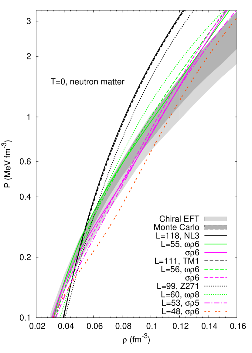
Figure 1: Neutron matter pressure, $P_{N}$, as a function of the density, for some of the models considered in this study. The coloured bands are the results from Hebeler et al. (2013) (light grey) and Gandolfi et al. (2012) (dark grey).

In Fig. 1, we show the EoS of pure neutron matter for a set of models from tables 1 and 2, and compare them with the result of microscopic calculations based on nuclear interactions derived from chiral effective field theory (EFT) Hebeler et al. (2013), or on realistic two- and three-nucleon interactions, using quantum Monte Carlo (MC) techniques Gandolfi et al. (2012). The band width indicates for each density the uncertainties of the calculation coming from the 3N interaction. At saturation density, this uncertainty is of the order of 5 MeV, $\sim 25-30\%$.

In Fig. 2 we plot the deviation of the neutron matter pressure for each model from the microscopic results of Hebeler et al. Hebeler et al. (2013) and Gandolfi et al. Gandolfi et al. (2012) data, in units of the pressure uncertainty $\Delta P$ of the microscopic calculations at each density, which we designate by $\sigma=\Delta P$. The light grey bands represent the microscopic calculation uncertainties, meaning that the points inside those bands are within the data limits. The dark grey bands correspond to twice the calculation uncertainties, $2\sigma$. Except for the head of each family and Z271$\omega\rho$8, all other models agree well with the results of Hebeler et al. (2013), and above $\rho=0.05$ fm^-3 with the MC results Gandolfi et al. (2012).

Models TM1, NL3 and Z271 have a too stiff neutron matter EoS. These models do not satisfy several other constraints imposed by experiments, see Dutra et al. (2014), in particular, the symmetry energy and/or its slope is too high, as well as the incompressibility. However, including the $\omega\rho$ or the $\sigma\rho$ terms, makes the symmetry energy softer, and we obtain some models that satisfy most of the constraints imposed in Dutra et al. (2014). We will not consider the $K_{\tau}$ constraint included in Dutra et al. (2014) because it has a large uncertainty associated to it. The NL3x and Z271x models have an incompressibility at saturation, $K$, just above the upper limit used in Khan et al. (2012); Dutra et al. (2014), $K=230\pm 40$ MeV, and TM1 only satisfies this constraint within 10%. However, the incompressibility of these models is within the range $250<K<315$ MeV predicted in Stone et al. (2014, 2016). Therefore, we consider that the $K$ constraint is satisfied.

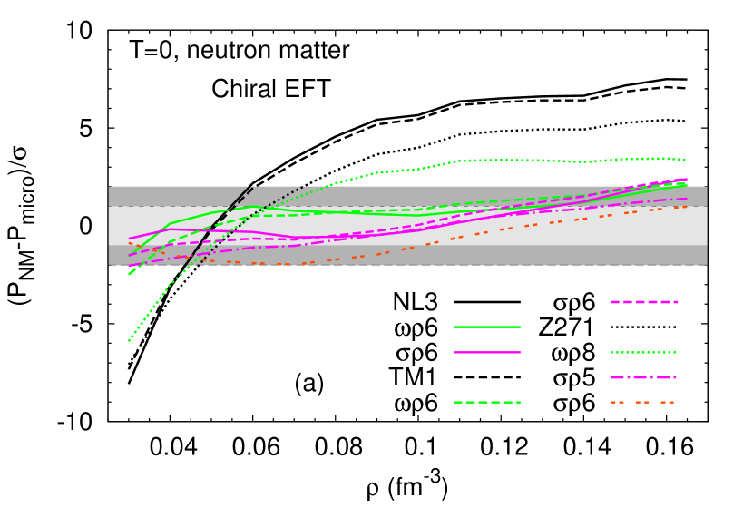
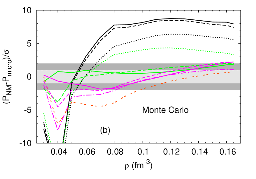
Figure 2: Difference between the neutron matter pressure for each model and the average pressure obtained from a chiral EFT Hebeler et al. (2013) (a) and Monte Carlo Gandolfi et al. (2012) (b) calculations, in units of the pressure uncertainty at each density, designated by $\sigma=\Delta P$. The grey bands represent the calculation uncertainty (light) and twice this uncertainty (dark). See text for more details.

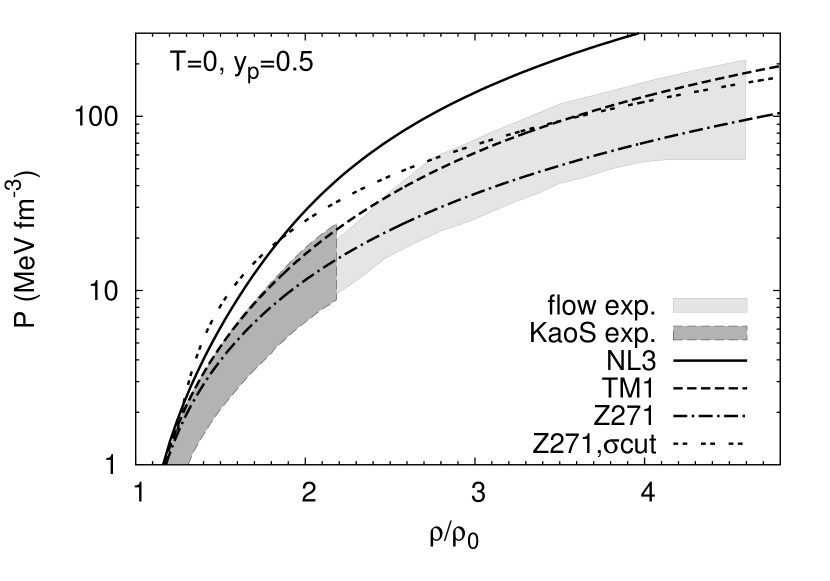
Figure 3: Symmmetric matter pressure, $P$, as a function of the density, for the models considered in this study. The coloured bands are the experimental results obtained from collective flow data in heavy-ion collisions Danielewicz et al. (2002) (light grey) and from the KaoS experiment Lynch et al. (2009); Fuchs (2006) (dark grey).

Constraints at suprasaturation densities from heavy ion collisions were also considered in Dutra et al. (2014). For reference, in Fig. 3, we show the symmetric matter pressure as a function of the density for the models considered in this study. This plot also includes a modified Z271 model, which has an extra effective potential that will be discussed later. We compare the different EoS with the experimental results obtained from collective flow data in heavy-ion collisions Danielewicz et al. (2002) and from the KaoS experiment Lynch et al. (2009); Fuchs (2006). Only Z271 and TM1 satisfy the constraints.

Summarizing the above discussion, models TM1$\omega\rho 6$, TM1$\sigma\rho 6$, and Z271$\sigma\rho 5-6$ satisfy the constraints imposed in Ref. Dutra et al. (2014), except the one in $K_{\tau}$, the constraints from neutron matter calculations and the ones from Refs. Stone et al. (2016, 2014). Models NL3$\omega\rho$6 and NL3$\sigma\rho 6$ only fail the flow and KaoS experiments.

III.2 Crust-core transition

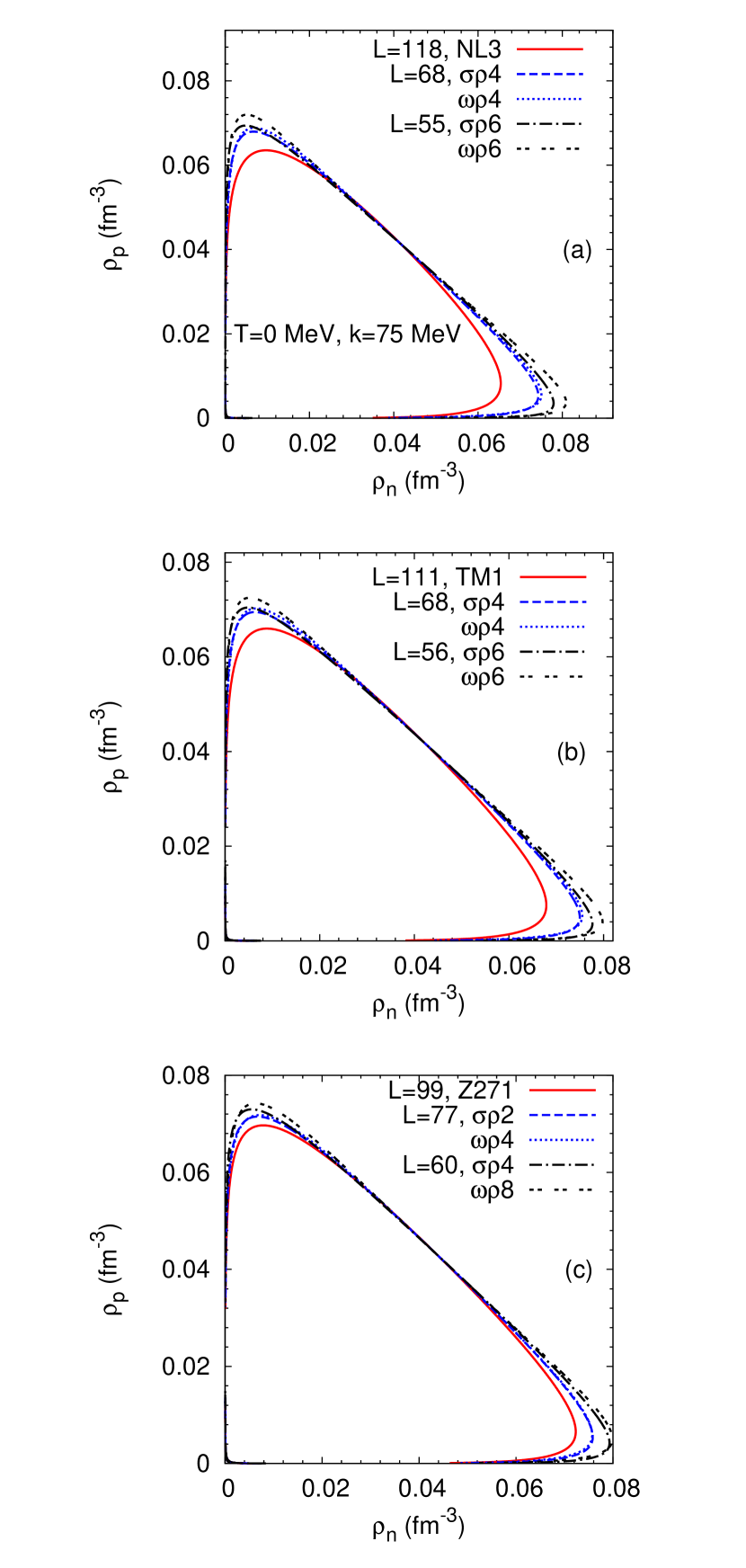
Figure 4: Spinodal regions for the models considered.

In Fig. 4, the dynamical spinodals for the six families under study are represented. They have been obtained solving the dispersion relation (26) for a zero energy mode, $\omega=0$, and taking the wave number $k=75$ MeV. We have considered this value of $k$ because the extension of the spinodal section is close to the envelope of all spinodal sections. For NL3 and TM1, we have considered, besides the head of the family, the two parametrizations with $\omega\rho$ or $\sigma\rho$ terms that give $L=55$ and 68 MeV; for Z271, we take the models with $L=76$ and 60 MeV. All the values of $L$ chosen are within the different constraints imposed in Dutra et al. (2014) for $L$. Some conclusions may be drawn from the figure: a) the larger $L$, the smaller the spinodal section, as discussed in previous works with different models Pais et al. (2010); b) the term $\omega\rho$ makes the spinodal section larger, except for the very large isospin asymmetries, both very neutron rich or very proton rich.

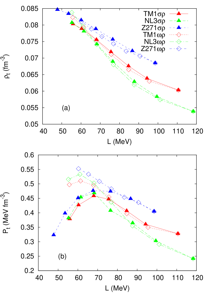
Figure 5: Crust-core transition (a) densities, $\rho_{t}$, and (b) pressure, $P_{t}$, as a function of the slope of the symmetry energy, $L$.

The crust-core transition density, $\rho_{t}$, is calculated from the crossing between the spinodal sections and the EoS for $\beta$-equilibrium matter. These densities are given in Tables 1 and 2 for all models under study, and are represented as a function of $L$ in Fig. 5, top panel. The crossing between the $\omega\rho$ and $\sigma\rho$ spinodals, for a given $L$, occurs close to the crossing of the $\beta$-equilibrium EoS with the spinodals and, therefore, the transition densities do not differ much, whether taking the $\omega\rho$ or the $\sigma\rho$ term. A difference, however, is seen when the transition pressures, $P_{t}$, are compared, see Fig. 5, bottom panel: while for the $\omega\rho$ terms, the transition pressure decreases monotonically with $L$, the exception being the lowest $L$ values for the TM1 and NL3 families, the $\sigma\rho$ terms gives rise to an increase of $P_{t}$ with $L$, until $L=70-80$ MeV, and only above this value, the pressure decreases with an increase of $L$.

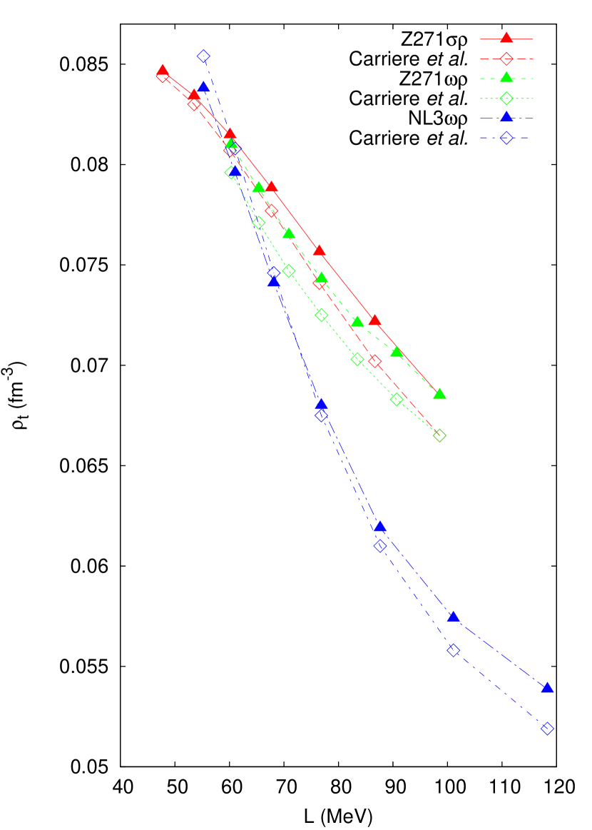
Figure 6: Crust-core transition densities, $\rho_{t}$, as a function of the slope of the symmetry energy, $L$, where we compare with the results obtained in Ref. Carriere et al. (2003).

For values of $L$ below 80 MeV, $P_{t}$ is generally larger in the models with the $\omega\rho$ term, and this difference may be as large as 25% for the smaller $L$ shown. This difference has direct implications in the moment of inertia of the crust, which is proportional to $P_{t}$, $I_{crust}\sim\frac{16\pi}{3}\frac{R_{t}^{6}P_{t}}{R_{s}}$ in lowest order Link et al. (1999); Shen et al. (2010); Piekarewicz et al. (2014), where $R_{t}$ is the crust thickness, and $R_{s}$ is the Schwarzschild radius. Besides the transition pressure, the moment of inertia of the crust also depends on the crust thickness. In the following, we will also see that the $\sigma\rho$ terms give rise to smaller crust thicknesses. This implies that smaller crust moments of inertia are expected, if the $\sigma\rho$ term is used to modify the symmetry energy.

In Fig. 6, we compare our results for the crust-core transition density with the ones obtained in Ref. Carriere et al. (2003), calculated within a relativistic random-phase-approximation Horowitz and Wehrberger (1991), for the Z271$\sigma\rho$ and $\omega\rho$ models, and for the NL3$\omega\rho$ family. For the Z271* models, we obtain slightly larger values for $\rho_{t}$, and this difference increases with increasing $L$, but even for the largest value of $L$, the difference is below 5%. For the NL3$\omega\rho$ models, the behaviour is slightly different: for $L<70$ MeV, our results are below the ones of Ref. Carriere et al. (2003), and for $L>70$ MeV, we get larger values, though the overall difference between them is below 5%.

III.3 Mass-radius curves for the NL3 families

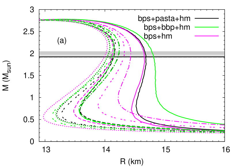
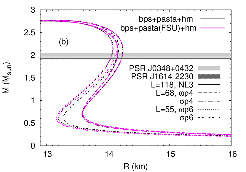
Figure 7: $M(R)$ relations for the NL3 models: (a) BPS EoS Baym et al. (1971) for the outer crust and the homogeneous matter EoS for the inner crust and core, bps+hm, (pink lines); the BPS+BBP Glendenning (2000) for the outer crust, and the homogeneous matter EoS for the inner crust and core, bps+bbp+hm, (green lines); and the BPS for the outer crust, the pasta configurations calculated from TF for the inner crust and the homogeneous matter EoS for the core, bps+pasta+hm (black lines); (b) BPS EoS for the outer crust, the pasta calculated from TF for the respective models (black lines), or for the FSU model (pink lines), for the inner crust, and the homogeneous matter EoS for the core. The horizontal bands indicate the mass uncertainties associated to the PSR J0348+0432 Antoniadis et al. (2013) and PSR J1614-2230 Fonseca et al. (2016) masses.

We calculate the mass-radius curves for the EoS under study, by integrating the Tolmann-Oppenheimer-Volkof equations Tolman (1939); Oppenheimer and Volkoff (1939), for relativistic spherical stars in hydrostatic equilibrium. In Fig. 7, the curves for the NL3 family are shown. In order to construct the EoS of stellar matter, we take, besides the EoS of the core, the BPS EoS for the outer crust, and several models for the inner crust: a) for models NL3$\omega\rho$ and $\sigma\rho$, we calculate the inner crust, within a Thomas-Fermi calculation Avancini et al. (2008); Grill et al. (2014). These inner crust EoS will also be considered when building the complete stellar matter EoS, within other models with similar properties; b) as an alternative that tests the use of a non-unified EoS, we consider the FSU inner crust EoS Grill et al. (2014), between the neutron drip density and the crust-core transition density, calculated within the dynamical spinodal method, for models with a similar slope $L$; c) we match directly the core EoS to the outer crust BPS EoS; d) the BPS plus Bethe-Baym-Pethick (BBP) EoS for densities below 0.01 fm^-3 is matched directly to the core EoS, as suggested in Glendenning (2000). Finally, we will estimate the error we introduce in quantities, such as the radius and mass, if the unified inner crust EoS is not used.

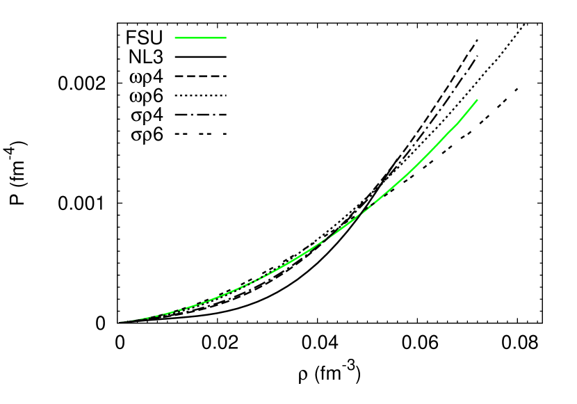
Figure 8: Inner crust EoSs considered in the present study.

In Fig. 8 and in the Appendix, we show the inner crust EoSs that we are using in this paper. Both the FSU, the NL3, and the NL3$\omega\rho 6$ inner crusts are given in Grill et al. (2014). In the top panel of Fig. 7, we compare the mass-radius curves for the stellar EoS obtained using the scenarios a) BPS plus an unified inner crust and core EoS (bps+pasta+hm), b) the inner crust EoS is replaced by the homogeneous matter EoS (bps+hm) and c) the BBP EoS is used for the low density inner crust EoS, and a transition to homogeneous matter occurs at $\sim 0.01$ fm^-3, below the crust-core transition (bps+bbp+hm). Totally neglecting the inner crust EoS (dashed curves) is a quite rough approximation for all EoS, except for NL3. Although the effect on the maximum mass is negligible, the same is not true for the radius. The families of stars with an unified inner crust-core EoS (solid lines) have larger (smaller) radii than the configurations without inner crust (dashed lines) for the NL3$\omega\rho$ (NL3$\sigma\rho$) models, see Tables 3 and 4. Including the BBP EoS between the neutron drip and $\rho=0.01$ fm^-3 (dotted lines) will generally reduce the differences with respect to the unified EoS, although the improvement depends a lot on the model.

Fig. 7 allows a comparison between mass-radius curves obtained with EoS whose density dependence of the symmetry energy is modified by means of a mixing $\omega\rho$ or $\sigma\rho$ term in the Lagrangian density. Within models with the same $L$, the $\sigma\rho$ models give slightly larger radii, the differences being larger for $M\gtrsim 1.4M_{\odot}$. For a $1.4M_{\odot}$ star, we have obtained a difference of $\sim 100$ m. These differences reflect themselves in the crust thickness, see Tables 3 and 4. The most critical approximation, giving rise to the largest error, occurs when the inner crust is completely neglected.

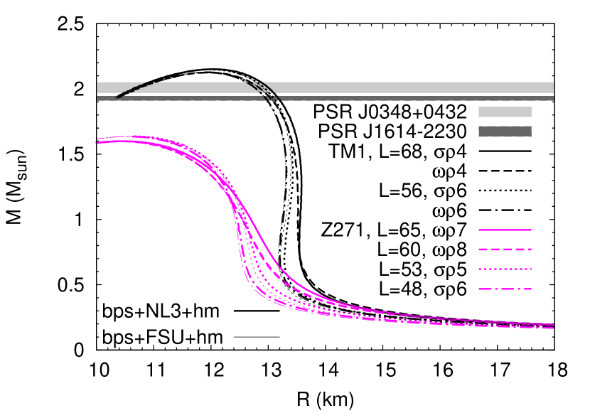
Figure 9: $M(R)$ relations for the all the TM1 and Z271 models considered: the stellar matter EoS contains the BPS outer crust EoS, the FSU inner crust (thin lines), the NL3$\omega\rho$ or the $\sigma\rho$ (thick lines) pasta phase EoS, and the core homogeneous matter EoS.

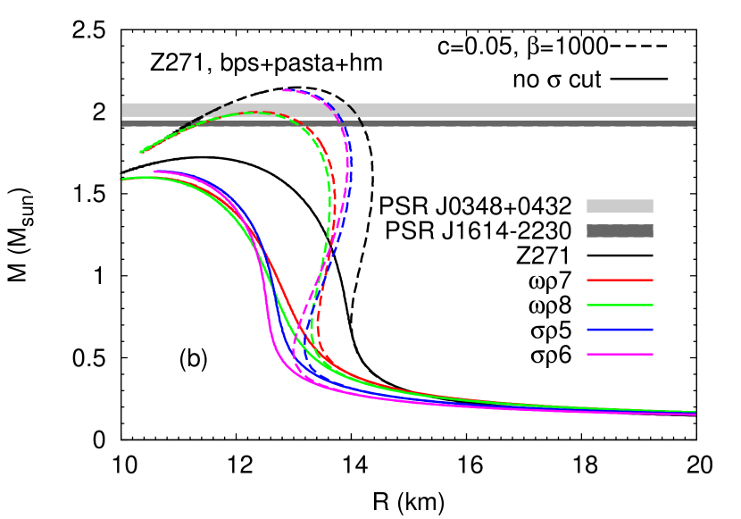
Figure 10: (a) Nucleon effective mass as a function of the density for isospin symmetric matter for the Z271 model with (dashed line) and without (solid line) the $\sigma$ cut potential. The black dot shows the effective mass at the nuclear saturation density, $\rho_{0}$; (b) $M(R)$ relations for the Z271 set of models, with (dashed lines) and without (solid lines) the $\sigma$ cut potential.

III.4 Stellar matter EoS

Most of the times, the inner crust EoS calculated within the same model is not available. In the previous section, we have tested the implications of not including the inner crust EoS, or only part of it. We now discuss the possible use of a inner crust EoS obtained for a different model. In the bottom panel of Fig. 7, we plot the mass-radius curves of stars obtained, considering for the inner crust the unified pasta calculation as before, and the inner crust EoS calculated for FSU, a model with the symmetry energy slope $L=60$ MeV, not far from the slope $L$ of NL3$\omega\rho 4,6$ and NL3$\sigma\rho 4,6$. Except for NL3$\sigma\rho 6$, where we obtain a difference of $\sim 50$ m ($\sim 40$ m) for a 1$M_{\odot}$ ( 1.4$M_{\odot}$) star, and for NL3$\omega\rho 6$, where we obtain $\sim 20$ m for a 1$M_{\odot}$ star, the error on the determination of the radius is negligible for all masses. This can be better seen in Tables 3 and 4.

Table 3: The radius and crust thickness of a 1.4 $M_{\odot}$ star, computed with an inner crust calculated within NL3$\sigma\rho$/NL3$\omega\rho$ and FSU, or using the BBP EoS, or without an inner crust (no ic) are shown. In all cases, we consider the BPS EoS for the outer crust.

Model		$L$ (MeV)		$R_{1.4M\odot}$	$\Delta R_{crust}$ (NL3)		$R_{1.4M\odot}$	$\Delta R_{crust}$ (FSU)		$R_{1.4M\odot}$	$\Delta R_{crust}$ (BBP)		$R_{1.4M\odot}$	$\Delta R_{crust}$ (no ic)
NL3		118		14.630	1.325		-	-		14.847	1.508		14.594	1.249
$\omega\rho$4		68		13.928	1.450		13.928	1.377		13.916	1.453		13.879	1.416
$\omega\rho$6		55		13.753	1.425		13.745	1.432		13.749	1.432		13.671	1.355
$\sigma\rho$4		68		13.982	1.441		13.983	1.388		13.977	1.445		14.313	1.781
$\sigma\rho$6		55		13.846	1.400		13.806	1.408		13.785	1.334		14.117	1.666

Table 4: The radius and crust thickness of a 1.0 $M_{\odot}$ star, computed with an inner crust calculated within NL3$\sigma\rho$/NL3$\omega\rho$ and FSU, or using the BBP EoS, or without an inner crust (no ic), are shown. In all cases, we consider the BPS EoS for the outer crust.

Model		$L$ (MeV)		$R_{1M\odot}$	$\Delta R_{crust}$ (NL3)		$R_{1M\odot}$	$\Delta R_{crust}$ (FSU)		$R_{1M\odot}$	$\Delta R_{crust}$ (BBP)		$R_{1M\odot}$	$\Delta R_{crust}$ (no ic)
NL3		118		14.547	1.956		-	-		14.870	2.230		14.489	1.850
$\omega\rho$4		68		13.681	2.077		13.686	1.979		13.665	2.079		13.621	2.035
$\omega\rho$6		55		13.423	2.020		13.402	2.020		13.410	2.025		13.300	1.913
$\sigma\rho$4		68		13.713	2.057		13.720	1.99		13.710	2.067		14.223	2.581
$\sigma\rho$6		55		13.511	1.987		13.457	1.993		13.423	1.885		13.924	2.386

Table 5: Maximum mass properties. For the TM1* and Z271* models, we used for the inner crust FSU, and NL3$\omega\rho$ and $\sigma\rho$. For TM1 and Z271, we used TM1. The radii, $R$, are given in km.

Model		$L$ (MeV)		$M_{g}$ (M⊙)		$M_{b}$ (M⊙)		$R$ (BPS)		$R$ (FSU)		$R$ (NL3)		$\epsilon_{0}$ (fm-4)		$\rho_{c}$ (fm-3)
NL3		118		2.779		3.384		13.289		-		13.300		4.409		0.669
$\omega\rho$4		68		2.753		3.376		13.017		13.031		13.022		4.520		0.689
$\omega\rho$6		55		2.758		3.391		12.994		13.005		13.014		4.496		0.687
$\sigma\rho$4		68		2.771		3.400		13.190		13.116		13.114		4.450		0.679
$\sigma\rho$6		55		2.773		3.409		13.141		13.070		13.079		4.469		0.682
TM1		111		2.183		2.544		12.494		12.386		-		5.345		0.851
$\omega\rho$4		68		2.125		2.488		12.140		11.950		11.955		5.653		0.904
$\omega\rho$6		56		2.127		2.496		11.973		11.892		11.893		5.663		0.907
$\sigma\rho$4		68		2.150		2.521		12.105		12.034		12.038		5.565		0.889
$\sigma\rho$6		56		2.148		2.523		12.019		11.977		11.992		5.578		0.893
Z271		99		1.722		1.944		11.554		11.425		-		6.470		1.066
$\omega\rho$7		65		1.599		1.807		10.544		10.466		10.466		7.804		1.277
$\omega\rho$8		60		1.599		1.809		10.435		10.406		10.417		7.850		1.285
$\sigma\rho$5		53		1.637		1.857		10.733		10.611		10.621		7.422		1.220
$\sigma\rho$6		48		1.635		1.857		10.653		10.553		10.571		7.463		1.228

The above discussion indicates that the determination of the radii of stars requires that some care is taken when matching the crust EoS to the core EoS. Non-unified EoS may give rise to large uncertainties. It is possible, however, to build an adequate non-unified EoS, if the inner crust EoS is properly chosen. We have shown that taking the inner crust EoS of a model with similar symmetry energy properties, as the ones of the EoS used for the core, allowed the determination of the radii of the family of stars with masses above $1\,M_{\odot}$ with an uncertainty below 50 m. The inclusion of the inner crust EoS has definitely a strong effect on the radius of low and intermediate mass neutron stars.

For the TM1 and Z271 families, we do not have an unified EoS for the inner crust. In order to test the above conclusion, we have built the stellar EoS taking for the inner crust, between the neutron drip density and the crust-core transition density, and calculated within the dynamical spinodal method, a) the FSU EoS (thin lines) and b) the EoS obtained for the NL3$\omega\rho$ (dashed lines) and NL3$\sigma\rho$ (solid lines) models, choosing the EoS that has the properties closer to the ones of each one of the models of the TM1 or Z271 familes (thick lines), see Fig. 9. Table 5 gives the correspondent maximum mass properties. In some cases, the curves (almost) coincide: this occurs for all models with $L>60$ MeV. Considering the two inner crust EoS, small differences occur for models with $L<60$ MeV, but the differences for the 1$M_{\odot}$ (1.4$M_{\odot}$) are never larger than 50 (30) m. This procedure to choose the inner crust EoS seems to be a quite robust alternative to the unified inner crust EoS.

Although the SNM and PNM properties of some of the Z271 models are in good agreement with experimental results or microscopic calculations, they predict a too small maximum mass star. This problem can be solved by introducing an extra effective potential, dependent on the $\sigma$ meson, that hinders the effective nucleon mass to stop decreasing at a density above the saturation density, as suggested in Maslov et al. (2015). In Figure 10, we show, in the top panel, the nucleon effective mass as a function of the density for the Z271 model, with and without the $\sigma$ cut potential, $\Delta U_{f}$, eq. 10 in Ref. Maslov et al. (2015), written as

$$\Delta U_{f} = \alpha\ln(1+\exp\left[\beta(g_{s}\phi-f)\right]),$$

$$f = f_{0}+c_{\sigma}(1-f_{0}).$$ (29)

We have used the parameters $\beta=1000$ and $c_{\sigma}=0.05$ to be able to get maximum masses of, at least, 2 $M_{\odot}$, as shown in the bottom panel (see also Ref. M. Dutra, O. Lourenço, and D. P. Menezes (2016), where they choose different parameters). $f_{0}$ and $\alpha$ have the same values as in Ref.Maslov et al. (2015), 0.2 and 4.822$\times 10^{-4}$ $m_{N}^{4}$, respectively. The stellar matter EoS were built using the BPS outer crust EoS, the most adequate NL3$\omega\rho$ or NL3$\sigma\rho$ inner crust EoS, and the homogeneous matter core EoS. The potential given in Eq. (III.4) does not allow constructing a EoS that simultaneously satisfies the $2M_{\odot}$ and the KaoS constrains, see Fig. 3.

We show in Figure 11 the mass-radius relation for the models that passed almost all constraints we considered: the ones from Ref. Dutra et al. (2014), the ones from Refs. Stone et al. (2016, 2014), the microscopic neutron matter calculations Hebeler et al. (2013); Gandolfi et al. (2012), and the 2$M_{\odot}$ observational constraint Antoniadis et al. (2013); Fonseca et al. (2016). We note that the Z271$\sigma\rho 5-6$ models fail this last constraint, however using the procedure of Ref. Maslov et al. (2015), we are able to get parametrizations Z271$\sigma\rho 5*-6*$ that describe 2$M_{\odot}$ stars. Models NL3$\omega\rho 6$, NL3$\sigma\rho 6$ and Z271$\sigma\rho 5*-6*$ fail the flow and KaoS experiments. In Table 6, we show the properties of the 1.4$M_{\odot}$ stars obtained with those models, together with the transition density and pressure. The following conclusions can be drawn: a) all models predict a similar transition density and have a similar symmetry energy slope; b) the $\sigma\rho$ models predict a lower transition pressure, $P_{t}\sim 0.36\pm 0.04$ MeVfm^-3, while for the $\omega\rho$ models the value is $P_{t}\sim 0.5$MeVfm^-3; c) the radius and crust thickness of the 1.4$M_{\odot}$ stars within the models that predict 2$M_{\odot}$ stars are in the interval $13.3\lesssim R_{1.4}\lesssim 13.9$ km and $1.3\lesssim\Delta R\lesssim 1.4$km, respectively.

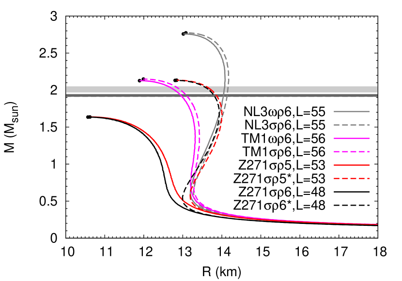
Figure 11: Mass-radius relation of the models that passed almost all the constraints we considered. The black dots represent the maximum mass star.

Table 6: Some properties of the 1.4$M_{\odot}$ stars of the models that passed almost all the constraints, computed with an inner crust, using NL3$\sigma\rho$ or NL3$\omega\rho$. The transition pressure, $P_{t}$, and density, $\rho_{t}$, to uniform matter are also shown.

Model		$L$ (MeV)		$R_{1.4M\odot}$ (km)		$\Delta R_{crust}$ (km)		$P_{t}$ (MeV/fm3)		$\rho_{t}$ (fm-3)
NL3$\omega\rho$6		55		13.753		1.425		0.516		0.084
NL3$\sigma\rho$6		55		13.846		1.400		0.382		0.081
TM1$\omega\rho$6		56		13.317		1.323		0.497		0.082
TM1$\sigma\rho$6		56		13.428		1.302		0.379		0.080
Z271$\sigma\rho$5		53		12.110		1.035		0.398		0.083
Z271$\sigma\rho 5^{*}$		53		13.914		1.419		0.398		0.083
Z271$\sigma\rho$6		48		12.001		0.995		0.323		0.085
Z271$\sigma\rho 6^{*}$		48		13.833		1.389		0.323		0.085

IV Conclusions

In the present work we have generalized the Vlasov formalism developed in previous works Avancini et al. (2005); Providência et al. (2006a); Pais et al. (2009, 2010) with the $\omega$, $\rho$, $\sigma$-meson terms, by including mixed terms, up to fourth order. The dispersion relation obtained allows the study of the isoscalar collective modes of nuclear matter, and the instability modes that drive the system at subsaturation densities to a non-homogeneous phase. The dynamical spinodal surface is determined as the locus of the zero frequency isoscalar mode. The knowledge of the dynamical spinodal and the $\beta$-equilibrium EoS is used to make a good estimation of the crust-core transition density of a neutron star.

We have applied the formalism developed to study several families of stars that differ by a mixed $\omega\rho$ or $\sigma\rho$ term which was introduced to modify the density dependence of the symmetry energy. We have analysed the dependence of the crust-core transition density, $\rho_{t}$, and pressure, $P_{t}$, with the slope $L$ of the model. We have confirmed previous results, in particular, an almost linear anti-correlation between $\rho_{t}$ and $L$, for both mixed $\omega\rho$ or $\sigma\rho$ terms. However, in a recent publication Pais et al. (2016), it has been shown that a non-linear $\sigma\rho$ term of the form $\sigma\rho^{2}$, instead of $\sigma^{2}\rho^{2}$, as we have considered in the present work, did not show this linear behavior with $L$. The behavior of $P_{t}$ is non-monotonic, as discussed in Ducoin et al. (2010, 2011), taking the $\sigma\rho$ family. However, if we consider only the $\omega\rho$ families, an anti-correlation of $P_{t}$ with $L$ is obtained. The largest transition pressures, largest crust thicknesses and smallest radii are obtained within the $\omega\rho$ families, see also Pais et al. (2016). For the $\sigma\rho$ families, $P_{t}$ increases (decreases) with $L$, for $L<70$ ($L>70$) MeV.

It was shown how the knowledge of the crust-core transition density enables the construction of the stellar EoS and the determination of the mass-radius curve for the family of stars, within a given model with a small radius uncertainty. For the outer crust, that extends up to the neutron drip density, the BPS EoS is considered. Between the neutron drip density and the crust-core transition density, the inner crust EoS should be taken. We have determined the inner crust EoS within a TF calculation for the $\omega\rho$ and $\sigma\rho$ NL3 family. It was shown that the error introduced in the calculation of the radius of a star with a mass above $1M_{\odot}$ is small, if the inner crust of a model with similar isovector saturation properties is used to describe the inner crust.

Since the Z21 family gives rise to a too soft EoS, a $\sigma$ dependent term was included in the Lagrangian density, as suggested in Maslov et al. (2015). This extra term does not change the model properties at saturation density and below, but hardens the EoS above saturation density, allowing the description of 2 $M_{\odot}$, but, at the same time, not satisfying the KaoS restrictions.

We propose a set of stellar matter EoS that satisfy well accepted saturation properties as well as constraints coming from microscopic neutron matter calculations, and from experimental results. All models predict a similar transition density of the order of $0.08$ fm^-3. However, there are differences in the transition pressure. The $\sigma\rho$ models predict a lower transition pressure than the $\omega\rho$ models. For the 1.4$M_{\odot}$ stars, these models predict, respectively, a radius of $13.6\pm 0.3$ km and a crust thickness of $1.36\pm 0.06$km. These values for $R_{1.4}$ are above the prediction of Lattimer and Steiner (2014) but within the prediction of Fortin et al. (2016). These crust thicknesses are $\sim 25\%$ smaller than the one obtained in Piekarewicz et al. (2014) for the NL3max, which is close to our parametrization NL3$\omega\rho$5. We have considered the NL3max parametrization and we have obtained, using our formalism, $P_{t}=0.530$ MeV/fm³ and $\rho_{t}=0.081$ fm^-3, just slightly below the corresponding quantities in Piekarewicz et al. (2014), respectively, 0.550 MeV/fm³ and 0.0826 fm^-3. However, for the crust thickness, we have obtained $\Delta R(M=1.4M_{\odot})=1.454$ km, that should be compared with $\Delta R(M=1.4M_{\odot})=1.990$ km in Piekarewicz et al. (2014). The possible origin of this large difference is the EoS used in Piekarewicz et al. (2014) for the inner crust EoS, a politropic that matches the BPS EoS at the neutron drip density and the homogeneous EoS at the crust-core transition. As we have shown in the present work, a non adequate choice of the inner crust may introduce large uncertainties in the radius of low mass stars, see also discussion in Fortin et al. (2016).

V Appendix

Table 7: Equation of state of the inner crust with pasta for the NL3$\omega\rho 4$, NL3$\sigma\rho 4$, and NL3$\sigma\rho 6$ models. The energy density, $\varepsilon$, and pressure, $P$, are in units of fm^-4. The pasta inner crust EoS for FSU and NL3$\omega\rho 6$ are given in Grill et al. (2014).

	NL3$\omega\rho 4$			NL3$\sigma\rho 4$			NL3$\sigma\rho 6$
$\rho$ (fm-3)	$\varepsilon$	P		$\varepsilon$	P		$\varepsilon$	P
0.0020	0.009529489093	0.9527332622$\times$10-5		0.009524920955	0.9071237400$\times$10-5		0.009525820613	0.9831396710$\times 10^{-5}$
0.0030	0.014300051145	0.1449370848$\times$10-4		0.014293017797	0.1424032234$\times$10-4		0.014294951223	0.1601402801$\times$10-4
0.0040	0.019072361290	0.1981482455$\times$10-4		0.019062936306	0.1981482455$\times$10-4		0.019066335633	0.2321020474$\times$10-4
0.0050	0.023846043274	0.2533865154$\times$10-4		0.023834312335	0.2579474858$\times$10-4		0.023839607835	0.3106518852$\times$10-4
0.0060	0.028620865196	0.3111586557$\times$10-4		0.028606912121	0.3197737897$\times$10-4		0.028614535928	0.3962964911$\times$10-4
0.0070	0.033396668732	0.3709578596$\times$10-4		0.033380579203	0.3856542753$\times$10-4		0.033390954137	0.4885291855$\times$10-4
0.0080	0.038173336536	0.4322774112$\times$10-4		0.038155212998	0.4540686496$\times$10-4		0.038168746978	0.5878567026$\times$10-4
0.0090	0.042950786650	0.4971443195$\times$10-4		0.042930707335	0.5255236465$\times$10-4		0.042947817594	0.6937723083$\times$10-4
0.0100	0.047728978097	0.5640384188$\times$10-4		0.047707032412	0.6015395775$\times$10-4		0.047728102654	0.8062758570$\times$10-4
0.0110	0.052507854998	0.6349865725$\times$10-4		0.052484132349	0.6811029743$\times$10-4		0.052509546280	0.9253675671$\times$10-4
0.0120	0.057287395000	0.7104958058$\times$10-4		0.057261981070	0.7652273052$\times$10-4		0.057292107493	0.1050540523$\times$10-3
0.0130	0.062067583203	0.7895524323$\times$10-4		0.062040548772	0.8549261111$\times$10-4		0.062075737864	0.1183315035$\times$10-3
0.0140	0.066848404706	0.8746902313$\times$10-4		0.066819831729	0.9501994646$\times$10-4		0.066860415041	0.1322170865$\times$10-3
0.0150	0.071629844606	0.9648958076$\times$10-4		0.071599796414	0.1050540523$\times$10-3		0.071646101773	0.1467614784$\times$10-3
0.0160	0.076411917806	0.1062196243$\times$10-3		0.076380468905	0.1157976367$\times$10-3		0.076432794333	0.1619646646$\times$10-3
0.0170	0.081194624305	0.1166591464$\times$10-3		0.081161834300	0.1272507070$\times$10-3		0.081220448017	0.1778773440$\times$10-3
0.0180	0.085977941751	0.1277574775$\times$10-3		0.085943877697	0.1392612321$\times$10-3		0.086009055376	0.1943474635$\times$10-3
0.0190	0.090761914849	0.1397173182$\times$10-3		0.090726628900	0.1521839440$\times$10-3		0.090798601508	0.2114763920$\times$10-3
0.0200	0.095546536148	0.1524880063$\times$10-3		0.095510080457	0.1659174886$\times$10-3		0.095589056611	0.2292641148$\times$10-3
0.0210	0.100331813097	0.1660695270$\times$10-3		0.100294232368	0.1803605264$\times$10-3		0.100380428135	0.2476093068$\times$10-3
0.0220	0.105117775500	0.1806645887$\times$10-3		0.105079092085	0.1957157365$\times$10-3		0.105172678828	0.2665626234$\times$10-3
0.0230	0.109904408455	0.1962225215$\times$10-3		0.109864674509	0.2119831624$\times$10-3		0.109965816140	0.2860733657$\times$10-3
0.0240	0.114691741765	0.2126419713$\times$10-3		0.114650979638	0.2290107223$\times$10-3		0.114759802818	0.3061415919$\times$10-3
0.0250	0.119479775429	0.2302269859$\times$10-3		0.119438014925	0.2471531916$\times$10-3		0.119554653764	0.3267672437$\times$10-3
0.0260	0.124268546700	0.2487241873$\times$10-3		0.124225787818	0.2661572071$\times$10-3		0.124350324273	0.3478490107$\times$10-3
0.0270	0.129058048129	0.2684376668$\times$10-3		0.129014313221	0.2860226959$\times$10-3		0.129146814346	0.3694882325$\times$10-3
0.0280	0.133848294616	0.2892660559$\times$10-3		0.133803606033	0.3070030943$\times$10-3		0.133944109082	0.3915328707$\times$10-3
0.0290	0.138639286160	0.3110066173$\times$10-3		0.138593643904	0.3289463930$\times$10-3		0.138742208481	0.4140842648$\times$10-3
0.0300	0.143431067467	0.3341154661$\times$10-3		0.143384456635	0.3517511941$\times$10-3		0.143541097641	0.4371930845$\times$10-3
0.0310	0.148223638535	0.3583898942$\times$10-3		0.148176059127	0.3757722152$\times$10-3		0.148340746760	0.4605046706$\times$10-3
0.0320	0.153017029166	0.3838805715$\times$10-3		0.152968466282	0.4008067772$\times$10-3		0.153141170740	0.4840695765$\times$10-3
0.0330	0.157811194658	0.4102834500$\times$10-3		0.157761648297	0.4266015312$\times$10-3		0.157942339778	0.5083946744$\times$10-3
0.0340	0.162606209517	0.4381559847$\times$10-3		0.162555649877	0.4537139030$\times$10-3		0.162744253874	0.5328211701$\times$10-3
0.0350	0.167402043939	0.4672447394$\times$10-3		0.167350441217	0.4818398156$\times$10-3		0.167546868324	0.5576530239$\times$10-3
0.0360	0.172198727727	0.4972963943$\times$10-3		0.172146052122	0.5110806087$\times$10-3		0.172350198030	0.5827890127$\times$10-3
0.0370	0.176996275783	0.5288176471$\times$10-3		0.176942497492	0.5410308950$\times$10-3		0.177154257894	0.6081783213$\times$10-3
0.0380	0.181794673204	0.5616059061$\times$10-3		0.181739777327	0.5723494687$\times$10-3		0.181958958507	0.6339224055$\times$10-3
0.0390	0.186593979597	0.5956103560$\times$10-3		0.186537876725	0.6046815543$\times$10-3		0.186764389277	0.6598691689$\times$10-3
0.0400	0.191394165158	0.6305776769$\times$10-3		0.191336825490	0.6381286075$\times$10-3		0.191570460796	0.6861706497$\times$10-3
0.0410	0.196195229888	0.6671160227$\times$10-3		0.196136608720	0.6722850958$\times$10-3		0.196377217770	0.7126749260$\times$10-3
0.0420	0.200997203588	0.7048706175$\times$10-3		0.200937271118	0.7078098715$\times$10-3		0.201184600592	0.7393818232$\times$10-3
0.0430	0.205800086260	0.7435374428$\times$10-3		0.205738782883	0.7443482173$\times$10-3		0.205992653966	0.7663421566$\times$10-3
0.0440	0.210603877902	0.7838258753$\times$10-3		0.210541129112	0.7819508319$\times$10-3		0.210801303387	0.7935052272$\times$10-3
0.0450	0.215408638120	0.8252799162$\times$10-3		0.215344354510	0.8203641628$\times$10-3		0.215610593557	0.8209216176$\times$10-3
0.0460	0.220214262605	0.8680008468$\times$10-3		0.220148459077	0.8600444999$\times$10-3		0.220420479774	0.8487434825$\times$10-3
0.0470	0.225020855665	0.9116340661$\times$10-3		0.224953413010	0.9007891058$\times$10-3		0.225230976939	0.8765652892$\times$10-3
0.0480	0.229828447104	0.9568381938$\times$10-3		0.229759275913	0.9425471653$\times$10-3		0.230042085052	0.9045898332$\times$10-3
0.0490	0.234636932611	0.1003258629$\times$10-2		0.234565988183	0.9850654751$\times$10-3		0.234853759408	0.9328678134$\times$10-3
0.0500	0.239446416497	0.1050844556$\times$10-2		0.239373609424	0.1028901315$\times$10-2		0.239666014910	0.9612977155$\times$10-3
0.0510	0.244256809354	0.1099342713$\times$10-2		0.244182094932	0.1073801308$\times$10-2		0.244478836656	0.9899811121$\times$10-3
0.0520	0.249068230391	0.1149259857$\times$10-2		0.248991489410	0.1119664288$\times$10-2		0.249292254448	0.1018968527$\times$10-2
0.0530	0.253880590200	0.1200494706$\times$10-2		0.253801763058	0.1166490139$\times$10-2		0.254106193781	0.1048057340$\times$10-2
0.0540	0.258693933487	0.1252894988$\times$10-2		0.258612930775	0.1214076183$\times$10-2		0.258920729160	0.1077298075$\times$10-2
0.0550	0.263508260250	0.1306410180$\times$10-2		0.263424992561	0.1263131737$\times$10-2		0.263735800982	0.1106893644$\times$10-2
0.0560	0.268323540688	0.1361090923$\times$10-2		0.268237978220	0.1312998240$\times$10-2		0.268551379442	0.1136742532$\times$10-2
0.0570	0.273139834404	0.1416582614$\times$10-2		0.273051828146	0.1363878255$\times$10-2		0.273367494345	0.1166743576$\times$10-2
0.0580	0.277957081795	0.1473594690$\times$10-2		0.277866572142	0.1415771898$\times$10-2		0.278184115887	0.1193450415$\times$10-2
0.0590	0.282775372267	0.1531822840$\times$10-2		0.282682240009	0.1468628179$\times$10-2		0.283001244068	0.1224211650$\times$10-2
0.0600	0.287594646215	0.1590811298$\times$10-2		0.287498801947	0.1522396924$\times$10-2		0.287818878889	0.1255124691$\times$10-2
0.0610	0.292414903641	0.1651167870$\times$10-2		0.292316287756	0.1577280345$\times$10-2		0.292637050152	0.1286341925$\times$10-2
0.0620	0.297236144543	0.1712639467$\times$10-2		0.297134667635	0.1632873435$\times$10-2		0.297455728054	0.1317913993$\times$10-2
0.0630	0.302058428526	0.1775073935$\times$10-2		0.301954001188	0.1689581317$\times$10-2		0.302274912596	0.1349739265$\times$10-2
0.0640	0.306881725788	0.1838724711$\times$10-2		0.306774199009	0.1747201430$\times$10-2		0.307094633579	0.1381919370$\times$10-2
0.0650	0.311706036329	0.1902932650$\times$10-2		0.311595320702	0.1802540966$\times$10-2		0.311914891005	0.1414707513$\times$10-2
0.0660	0.316531240940	0.1965164440$\times$10-2		0.316417217255	0.1862238860$\times$10-2		0.316735535860	0.1447597286$\times$10-2
0.0670	0.321357458830	0.2031500917$\times$10-2		0.321240127087	0.1922595431$\times$10-2		0.321556776762	0.1480993466$\times$10-2
0.0680	0.326184719801	0.2099307254$\times$10-2		0.326063960791	0.1983914990$\times$10-2		0.326378494501	0.1514491159$\times$10-2
0.0690	0.331013083458	0.2167164115$\times$10-2		0.330888777971	0.2045741305$\times$10-2		0.331200808287	0.1548850443$\times$10-2
0.0700	0.335842400789	0.2236136002$\times$10-2		0.335714370012	0.2098242985$\times$10-2		0.336023390293	0.1571097760$\times$10-2
0.0710	0.340671092272	0.2294718986$\times$10-2		0.340540796518	0.2163312631$\times$10-2		0.340846419334	0.1606267877$\times$10-2
0.0720	0.345502316952	0.2361764899$\times$10-2		0.345368176699	0.2228483791$\times$10-2		0.345669955015	0.1643870375$\times$10-2
0.0730							0.350494056940	0.1680915593$\times$10-2
0.0740							0.355318605900	0.1718517975$\times$10-2
0.0750							0.360143750906	0.1756627345$\times$10-2
0.0760							0.364969402552	0.1795750228$\times$10-2
0.0770							0.369795531034	0.1834822469$\times$10-2
0.0780							0.374622225761	0.1874604146$\times$10-2
0.0790							0.379449486732	0.1914335182$\times$10-2
0.0800							0.384277373552	0.1953660743$\times$10-2

References

- Tang et al. (1981) H. H. K. Tang, C. H. Dasso, H. Esbensen, R. A. Broglia, and A. Winther, Physics Letters B 101, 10 (1981).
- Jin et al. (1989) X. Jin, Y. X. Zhang, and M. Sano, Nucl. Phys. A 506, 655 (1989).
- Ko and Li (1988) C. M. Ko and Q. Li, Phys. Rev. C 37, 2270 (1988).
- Ko and Li (1987) C. M. Ko and Q. Li, Phys. Rev. Lett. 59, 1084 (1987).
- Li and Ko (1988) Q. Li and C. M. Ko, Phys. Lett. A 3, 465 (1988).
- Nielsen et al. (1991) M. Nielsen, C. Providência, and J. da Providência, Phys. Rev. C 44, 209 (1991).
- Nielsen et al. (1993) M. Nielsen, C. Providência, and J. da Providência, Phys. Rev. C 47, 200 (1993).
- Avancini et al. (2005) S. S. Avancini, L. Brito, D. P. Menezes, and C. Providência, Phys. Rev. C 71, 044323 (2005).
- Providência et al. (2006a) C. Providência, L. Brito, A. M. S. Santos, D. P. Menezes, and S. S. Avancini, Phys. Rev. C 74, 045802 (2006a).
- Pais et al. (2009) H. Pais, A. Santos, and C. Providência, Phys. Rev. C 80, 045808 (2009).
- Pais et al. (2010) H. Pais, A. Santos, L. Brito, and C. Providência, Phys. Rev. C 82, 025801 (2010).
- Santos et al. (2008) A. M. Santos, L. Brito, and C. Providência, Phys. Rev. C 77, 045805 (2008).
- Avancini et al. (2010) S. S. Avancini, S. Chiacchiera, D. P. Menezes, and C. Providência, Phys. Rev. C 82, 055807 (2010).
- Avancini et al. (2012) S. S. Avancini, S. Chiacchiera, D. P. Menezes, and C. Providência, Phys. Rev. C 85, 059904(E) (2012).
- Pethick et al. (1995) C. J. Pethick, D. J. Ravenhall, and C. P. Lorenz, Nucl. Phys. A 584, 675 (1995).
- Fortin et al. (2016) M. Fortin, C. Providência, A. R. Raduta, F. Gulminelli, J. L. Zdunik, P. Haensel, and M. Bejger, ArXiv e-prints (2016), arXiv:1604.01944 [astro-ph.SR] .
- Baym et al. (1971) G. Baym, C. Pethick, and P. Sutherland, Astrophys. J. 170, 299 (1971).
- Haensel and Pichon (1994) P. Haensel and B. Pichon, Astron. Astrophys. 283, 313 (1994).
- Rüster et al. (2006) S. B. Rüster, M. Hempel, and J. Schaffner-Bielich, Phys. Rev. C 73, 035804 (2006).
- Ravenhall et al. (1983) D. G. Ravenhall, C. J. Pethick, and J. R. Wilson, Phys. Rev. Lett. 50, 2066 (1983).
- Watanabe et al. (2009) G. Watanabe, H. Sonoda, T. Maruyama, K. Sato, K. Yasuoka, and T. Ebisuzaki, Phys. Rev. Lett. 103, 121101 (2009).
- Horowitz et al. (2005) C. J. Horowitz, M. A. Pérez-García, D. K. Berry, and J. Piekarewicz, Phys. Rev. C 72, 035801 (2005).
- Schneider et al. (2016) A. S. Schneider, D. K. Berry, M. E. Caplan, C. J. Horowitz, and Z. Lin, ArXiv e-prints (2016), arXiv:1602.03215 [nucl-th] .
- Dorso et al. (2012) C. O. Dorso, P. A. Giménez Molinelli, and J. A. López, Phys. Rev. C 86, 055805 (2012).
- Newton and Stone (2009) W. G. Newton and J. R. Stone, Phys. Rev. C 79, 055801 (2009).
- Pais and Stone (2012) H. Pais and J. R. Stone, Phys. Rev. Lett. 109, 151101 (2012).
- Maruyama et al. (2005) T. Maruyama, T. Tatsumi, D. Voskresensky, T. Tanigawa, and S. Chiba, Phys. Rev. C 72, 015802 (2005).
- Avancini and Bertolino (2015) S. S. Avancini and B. P. Bertolino, International Journal of Modern Physics E 24, 1550078 (2015).
- Okamoto et al. (2013) M. Okamoto, T. Maruyama, K. Yabana, and T. Tatsumi, Phys. Rev. C 88, 025801 (2013).
- Pons et al. (2013) J. A. Pons, D. Viganò, and N. Rea, Nature Phys. 9, 431 (2013).
- Tolman (1939) R. C. Tolman, Physical Review 55, 364 (1939).
- Oppenheimer and Volkoff (1939) J. R. Oppenheimer and G. M. Volkoff, Physical Review 55, 374 (1939).
- Hebeler et al. (2013) K. Hebeler, J. M. Lattimer, C. J. Pethick, and A. Schwenk, Astrophys. J. 773, 11 (2013).
- Gandolfi et al. (2012) S. Gandolfi, J. Carlson, and S. Reddy, Phys. Rev. C 85, 032801 (2012).
- Danielewicz et al. (2002) P. Danielewicz, R. Lacey, and W. G. Lynch, Science 298, 1592 (2002).
- Lynch et al. (2009) W. G. Lynch, M. B. Tsang, Y. Zhang, P. Danielewicz, M. Famiano, Z. Li, and A. W. Steiner, Prog. Part. Nucl. Phys. 62, 427 (2009).
- Tsang et al. (2012) M. B. Tsang, J. R. Stone, F. Camera, P. Danielewicz, S. Gandolfi, K. Hebeler, C. J. Horowitz, J. Lee, W. G. Lynch, Z. Kohley, R. Lemmon, P. Möller, T. Murakami, S. Riordan, X. Roca-Maza, F. Sammarruca, A. W. Steiner, I. Vidaña, and S. J. Yennello, Phys. Rev. C 86, 015803 (2012).
- Demorest et al. (2010) P. B. Demorest, T. Pennucci, S. M. Ransom, M. S. E. Roberts, and J. W. T. Hessels, Nature 467, 1081 (2010).
- Antoniadis et al. (2013) J. Antoniadis, P. C. C. Freire, N. Wex, T. M. Tauris, R. S. Lynch, M. H. van Kerkwijk, M. Kramer, C. Bassa, V. S. Dhillon, T. Driebe, J. W. T. Hessels, V. M. Kaspi, V. I. Kondratiev, N. Langer, T. R. Marsh, M. A. McLaughlin, T. T. Pennucci, S. M. Ransom, I. H. Stairs, J. van Leeuwen, J. P. W. Verbiest, and D. G. Whelan, Science 340, 448 (2013).
- Fonseca et al. (2016) E. Fonseca, T. T. Pennucci, J. A. Ellis, I. H. Stairs, D. J. Nice, S. M. Ransom, P. B. Demorest, Z. Arzoumanian, K. Crowter, T. Dolch, R. D. Ferdman, M. E. Gonzalez, G. Jones, M. L. Jones, M. T. Lam, L. Levin, M. A. McLaughlin, K. Stovall, J. K. Swiggum, and W. Zhu, ArXiv e-prints (2016), arXiv:1603.00545 [astro-ph.HE] .
- Barret et al. (2013) D. Barret, K. Nandra, X. Barcons, A. Fabian, J. W. den Herder, L. Piro, M. Watson, J. Aird, G. Branduardi-Raymont, M. Cappi, F. Carrera, A. Comastri, E. Costantini, J. Croston, A. Decourchelle, C. Done, M. Dovciak, S. Ettori, A. Finoguenov, A. Georgakakis, P. Jonker, J. Kaastra, G. Matt, C. Motch, P. O’Brien, G. Pareschi, E. Pointecouteau, G. Pratt, G. Rauw, T. Reiprich, J. Sanders, S. Sciortino, R. Willingale, and J. Wilms, in SF2A-2013 Proceedings, edited by L. Cambresy, F. Martins, E. Nuss, and A. Palacios (2013) pp. 447–453.
- Lalazissis et al. (1997) G. A. Lalazissis, J. König, and P. Ring, Phys. Rev. C 55, 540 (1997).
- Lattimer (2012) J. M. Lattimer, Annu. Rev. Nucl. Part. Sci. 62, 485 (2012).
- Weissenborn et al. (2012) S. Weissenborn, D. Chatterjee, and J. Schaffner-Bielich, Nucl. Phys. A 881, 62 (2012).
- Bonanno and Sedrakian (2012) L. Bonanno and A. Sedrakian, Astron. Astrophys. 539, A16 (2012).
- Horowitz and Piekarewicz (2001) C. J. Horowitz and J. Piekarewicz, Phys. Rev. Lett. 86, 5647 (2001).
- Carriere et al. (2003) J. Carriere, C. J. Horowitz, and J. Piekarewicz, Astrophys. J. 593, 463 (2003).
- Sugahara and Toki (1994) Y. Sugahara and H. Toki, Nucl. Phys. A 579, 557 (1994).
- Shen et al. (2011) G. Shen, C. J. Horowitz, and E. O’Connor, Phys. Rev. C 83, 065808 (2011).
- Maslov et al. (2015) K. A. Maslov, E. E. Kolomeitsev, and D. N. Voskresensky, Phys. Rev. C 92, 052801 (2015).
- Link et al. (1999) B. Link, R. I. Epstein, and J. M. Lattimer, Phys. Rev. Lett. 83, 3362 (1999).
- Chamel (2013) N. Chamel, Phys. Rev. Lett. 110, 011101 (2013).
- Andersson et al. (2012) N. Andersson, K. Glampedakis, W. Ho, and C. Espinoza, Phys. Rev. Lett. 109, 241103 (2012).
- Piekarewicz et al. (2014) J. Piekarewicz, F. J. Fattoyev, and C. J. Horowitz, Phys. Rev. C 90, 015803 (2014).
- Dutra et al. (2014) M. Dutra, O. Lourenço, S. S. Avancini, B. V. Carlson, A. Delfino, D. P. Menezes, C. Providência, S. Typel, and J. R. Stone, Phys. Rev. C 90, 055203 (2014).
- Pais et al. (2016) H. Pais, A. Sulaksono, B. K. Agrawal, and C. Providência, Phys. Rev. C 93, 045802 (2016).
- Ducoin et al. (2010) C. Ducoin, J. Margueron, and C. Providência, Europhysics Letters 91, 32001 (2010).
- Ducoin et al. (2011) C. Ducoin, J. Margueron, C. Providência, and I. Vidaña, Phys. Rev. C 83, 045810 (2011).
- Furnstahl et al. (1996) R. J. Furnstahl, B. D. Serot, and H. B. Tang, Nucl. Phys. A 598, 539 (1996).
- Furnstahl et al. (1997) R. J. Furnstahl, B. D. Serot, and H. B. Tang, Nucl. Phys. A 615, 441 (1997).
- Sulaksono and Kasmudin (2009) A. Sulaksono and Kasmudin, Phys. Rev. C 80, 054317 (2009).
- Agrawal (2010) B. K. Agrawal, Phys. Rev. C 81, 034323 (2010).
- Walecka (1974) J. D. Walecka, Ann. Phys. 83, 491 (1974).
- Avancini et al. (2004) S. S. Avancini, L. Brito, D. P. Menezes, and C. Providência, Phys. Rev. C 70, 015203 (2004).
- Providência et al. (2006b) C. Providência, L. Brito, S. S. Avancini, D. P. Menezes, and P. Chomaz, Phys. Rev. C 73, 025805 (2006b).
- Sumiyoshi et al. (1995) K. Sumiyoshi, H. Kuwabara, and H. Toki, Nuclear Physics A 581, 725 (1995).
- Vidaña et al. (2009) I. Vidaña, C. Providência, A. Polls, and A. Rios, Phys. Rev. C 80, 045806 (2009).
- Khan et al. (2012) E. Khan, J. Margueron, and I. Vidaña, Phys. Rev. Lett. 109, 092501 (2012).
- Stone et al. (2014) J. R. Stone, N. J. Stone, and S. A. Moszkowski, Phys. Rev. C 89, 044316 (2014).
- Stone et al. (2016) J. R. Stone, P. A. M. Guichon, P. G. Reinhard, and A. W. Thomas, Phys. Rev. Lett. 116, 092501 (2016).
- Fuchs (2006) C. Fuchs, Prog. Part. Nucl. Phys. 56, 1 (2006).
- Shen et al. (2010) G. Shen, C. J. Horowitz, and S. Teige, Phys. Rev. C 82, 045802 (2010).
- Horowitz and Wehrberger (1991) C. J. Horowitz and K. Wehrberger, Nuclear Physics A 531, 665 (1991).
- Glendenning (2000) N. K. Glendenning, Compact Stars (New York: Springer, 2000).
- Avancini et al. (2008) S. S. Avancini, D. P. Menezes, M. D. Alloy, J. R. Marinelli, M. M. W. Moraes, and C. Providência, Phys. Rev. C 78, 015802 (2008).
- Grill et al. (2014) F. Grill, H. Pais, C. Providência, I. Vidaña, and S. S. Avancini, Phys. Rev. C 90, 045803 (2014).
- M. Dutra, O. Lourenço, and D. P. Menezes (2016) M. Dutra, O. Lourenço, and D. P. Menezes, Phys. Rev. C 93, 025806 (2016).
- Lattimer and Steiner (2014) J. M. Lattimer and A. W. Steiner, European Physical Journal A 50, 40 (2014).