Uncertainty principles for inverse source problems, far field splitting and data completion

Abstract

Starting with far field data of time-harmonic acoustic or electromagnetic waves radiated by a collection of compactly supported sources in two-dimensional free space, we develop criteria and algorithms for the recovery of the far field components radiated by each of the individual sources, and the simultaneous restoration of missing data segments. Although both parts of this inverse problem are severely ill-conditioned in general, we give precise conditions relating the wavelength, the diameters of the supports of the individual source components and the distances between them, and the size of the missing data segments, which guarantee that stable recovery in presence of noise is possible. The only additional requirement is that a priori information on the approximate location of the individual sources is available. We give analytic and numerical examples to confirm the sharpness of our results and to illustrate the performance of corresponding reconstruction algorithms, and we discuss consequences for stability and resolution in inverse source and inverse scattering problems.

Mathematics subject classifications (MSC2010): 35R30, (65N21)
Keywords: Inverse source problem, Helmholtz equation, uncertainty principles, far field splitting, data completion, stable recovery
Short title: Uncertainty principles for inverse source problems

1 Introduction

In signal processing, a classical uncertainty principle limits the time-bandwidth product $|T||W|$ of a signal, where $|T|$ is the measure of the support of the signal $\phi(t)$, and $|W|$ is the measure of the support of its Fourier transform $\widehat{\phi}(\omega)$ (cf., e.g., [7]). A very elementary formulation of that principle is

$$|\langle\phi,\psi\rangle|\,\leq\,\sqrt{|T||W|}\|\phi\|_{2}\|\psi\|_{2}$$ (1.1)

whenever $\operatorname{supp}\phi\subseteq T$ and $\operatorname{supp}\widehat{\psi}\subseteq W$ .

In the inverse source problem, the far field radiated by a source $f$ is its restricted (to the unit sphere) Fourier transform, and the operator that maps the restricted Fourier transform of $f(x)$ to the restricted Fourier transform of its translate $f(x+c)$ is called the far field translation operator. We will prove an uncertainty principle analogous to (1.1), where the role of the Fourier transform is replaced by the far field translation operator. Combining this principle with a regularized Picard criterion, which characterizes the non-evanescent (i.e., detectable) far fields radiated by a (limited power) source supported in a ball provides simple proofs and extensions of several results about locating the support of a source and about splitting a far field radiated by well-separated sources into the far fields radiated by each source component.

We also combine the regularized Picard criterion with a more conventional uncertainty principle for the map from a far field in $L^{2}(S^{1})$ to its Fourier coefficients. This leads to a data completion algorithm which tells us that we can deduce missing data (i.e. on part of $S^{1}$) if we know a priori that the source has small support. All of these results can be combined so that we can simultaneously complete the data and split the far fields into the components radiated by well-separated sources. We discuss both $l^{2}$ (least squares) and $l^{1}$ (basis pursuit) algorithms to accomplish this.

Perhaps the most significant point is that all of these algorithms come with bounds on their condition numbers (both the splitting and data completion problems are linear) which we show are sharp in their dependence on geometry and wavenumber. These results highlight an important difference between the inverse source problem and the inverse scattering problem. The conditioning of the linearized inverse scattering problem does not depend on wavenumber, which means that the conditioning does not deteriorate as we increase the wavenumber in order to increase resolution. The conditioning for splitting and data completion for the inverse source problem does, however, deteriorate with increased wavenumber, which means the dynamic range of the sensors must increase with wavenumber to obtain higher resolution.

We note that applications of classical uncertainty principles for the one-dimensional Fourier transform to data completion for band-limited signals have been developed in [7]. In this classical setting a problem that is somewhat similar to far field splitting is the representation of highly sparse signals in overcomplete dictionaries. Corresponding stability results for basis pursuit reconstruction algorithms have been established in [6].

The numerical algorithms for far field splitting that we are going to discuss have been developed and analyzed in [9, 10]. The novel mathematical contribution of the present work is the stability analysis for these algorithms based on new uncertainty principles, and their application to data completion. For alternate approaches to far field splitting that however, so far, lack a rigorous stability analysis we refer to [12, 22] (see also [11] for a method to separate time-dependent wave fields due to multiple sources).

This paper is organized as follows. In the next section we provide the theoretical background for the direct and inverse source problem for the two-dimensional Helmholtz equation with compactly supported sources. In section 3 we discuss the singular value decomposition of the restricted far field operator mapping sources supported in a ball to their radiated far fields, and we formulate the regularized Picard criterion to characterize non-evanescent far fields. In section 4 we discuss uncertainty principles for the far field translation operator and for the Fourier expansion of far fields, and in section 5 we utilize those to analyze the stability of least squares algorithms for far field splitting and data completion. Section 6 focuses on corresponding results for ${l^{1}}$ algorithms. Consequences of these stability estimates related to conditioning and resolution of reconstruction algorithms for inverse source and inverse scattering problems are considered in section 7, and in section 8–9 we provide some analytic and numerical examples.

2 Far fields radiated by compactly supported sources

Suppose that $f\in L^{2}_{0}({\mathbb{R}}^{2})$ represents a compactly supported acoustic or electromagnetic source in the plane. Then the time-harmonic wave $v\in H^{1}_{\mathrm{loc}}({\mathbb{R}}^{2})$ radiated by $f$ at wave number $k>0$ solves the source problem for the Helmholtz equation

$$-\Delta v-k^{2}v\,=\,k^{2}g\qquad\text{in ${\mathbb{R}}^{2}$}\,,$$

and satisfies the Sommerfeld radiation condition

$$\lim_{r\to\infty}\sqrt{r}\Bigl{(}\frac{\partial v}{\partial r}-\mathrm{i}kv\Bigr{)}\,=\,0\,,\qquad r=|x|\,.$$

We include the extra factor of $k^{2}$ on the right hand side so that both $v$ and $g$ scale (under dilations) as functions; i.e., if $u(x)=v(kx)$ and $f(x)=g(kx)$, then

$$-\Delta u-u\,=\,f\qquad\text{in ${\mathbb{R}}^{2}$}\qquad\text{and}\qquad\lim_{r\to\infty}\sqrt{r}\Bigl{(}\frac{\partial u}{\partial r}-\mathrm{i}u\Bigr{)}\,=\,0\,.$$ (2.1)

With this scaling, distances are measured in wavelengths, and this allows us to set $k=1$ in our calculations, and then easily restore the dependence on wavelength when we are done.

The fundamental solution of the Helmholtz equation (with $k=1$) in two dimensions is

$$\Phi(x)\,:=\,\frac{\mathrm{i}}{4}H^{(1)}_{0}(|x|)\,,\qquad x\in{\mathbb{R}}^{2}\setminus\{0\}\,,$$

so the solution to (2.1) can be written as a volume potential

$$u(x)\,=\,\int_{{\mathbb{R}}^{2}}\Phi(x-y)f(y)\,\operatorname{d\!}y\,,\qquad x\in{\mathbb{R}}^{2}\,.$$

The asymptotics of the Hankel function tell us that

$$u(x)\,=\,\frac{e^{\frac{\mathrm{i}\pi}{4}}}{\sqrt{8\pi}}\frac{e^{\mathrm{i}r}}{\sqrt{r}}\alpha(\theta_{x})+O\left(r^{-\frac{3}{2}}\right)\qquad\text{as $r\to\infty$\,,}$$

where $x=r\theta_{x}$ with $\theta_{x}\in S^{1}$, and

$$\alpha(\theta_{x})\,=\,\int_{{\mathbb{R}}^{2}}e^{-\mathrm{i}\theta_{x}\cdot y}f(y)\,\operatorname{d\!}y\,.$$ (2.2)

The function $\alpha$ is called the far field radiated by the source $f$, and equation (2.2) shows that the far field operator $\mathcal{F}$, which maps $f$ to $\alpha$ is a restricted Fourier transform, i.e.

$$\mathcal{F}:\,L^{2}_{0}({\mathbb{R}}^{2})\to L^{2}(S^{1})\,,\quad\mathcal{F}f\,:=\,\widehat{f}\big{|}_{S^{1}}\,.$$ (2.3)

The goal of the inverse source problem is to deduce properties of an unknown source $f\in L^{2}_{0}({\mathbb{R}}^{2})$ from observations of the far field. Clearly, any compactly supported source with Fourier transform that vanishes on the unit circle is in the nullspace $\mathcal{N}(\mathcal{F})$ of the far field operator. We call $f\in\mathcal{N}(\mathcal{F})$ a non-radiating source because a corollary of Rellich’s lemma and unique continuation is that, if the far field vanishes, then the wave $u$ vanishes on the unbounded connected component of the complement of the support of $f$. The nullspace of $\mathcal{F}$ is exactly

$$\mathcal{N}(\mathcal{F})\,=\,\{g=-\Delta v-v\;|\;v\in H^{2}_{0}({\mathbb{R}}^{2})\}\,.$$

Neither the source $f$ nor its support is uniquely determined by the far field, and, as non-radiating sources can have arbitrarily large supports, no upper bound on the support is possible. There are, however, well defined notions of lower bounds. We say that a compact set $\Omega\subseteq{\mathbb{R}}^{2}$ carries $\alpha$, if every open neighborhood of $\Omega$ supports a source $f\in L^{2}_{0}({\mathbb{R}}^{2})$ that radiates $\alpha$. The convex scattering support $\mathscr{C}(\alpha)$ of $\alpha$, as defined in [18] (see also [19, 24]), is the intersection of all compact convex sets that carry $\alpha$. The set $\mathscr{C}(\alpha)$ itself carries $\alpha$, so that $\mathscr{C}(\alpha)$ is the smallest convex set which carries the far field $\alpha$, and the convex hull of the support of the “true” source $f$ must contain $\mathscr{C}(\alpha)$. Because two disjoint compact sets with connected complements cannot carry the same far field pattern (cf. [24, lemma 6]), it follows that $\mathscr{C}(\alpha)$ intersects any connected component of $\operatorname{supp}(f)$, as long as the corresponding source component is not non-radiating.

In [24], an analogous notion, the UWSCS support, was defined, showing that any far field with a compactly supported source is carried by a smallest union of well-separated convex sets (well-separated means that the distance between any two connected convex components is strictly greater than the diameter of any component). A corollary is that it makes theoretical sense to look for the support of a source with components that are small compared to the distance between them.

Here, as in previous investigations [9, 10], we study the well-posedness issues surrounding numerical algorithms to compute that support.

3 A regularized Picard criterion

If we consider the restriction of the source to far field map $\mathcal{F}$ from (2.3) to sources supported in the ball $B_{R}(0)$ of radius $R$ centered at the origin, i.e.,

$$\mathcal{F}_{B_{R}(0)}:\,L^{2}(B_{R}(0))\to L^{2}(S^{1})\,,\quad\mathcal{F}_{B_{R}(0)}f\,:=\,\widehat{f}\big{|}_{S^{1}}\,,$$ (3.1)

we can write out a full singular value decomposition. We decompose $f\in{L^{2}}(B_{R}(0))$ as

$$f(x)\,=\,\biggl{(}\sum_{n=-\infty}^{\infty}f_{n}\,\mathrm{i}^{n}J_{n}(|x|)e^{\mathrm{i}n\varphi_{x}}\biggr{)}\;\oplus f_{\mathrm{NR}}(x)\,,\qquad x=|x|(\cos\varphi_{x},\sin\varphi_{x})\in B_{R}(0)\,,$$

where $\mathrm{i}^{n}J_{n}(|x|)e^{\mathrm{i}n\varphi_{x}}$, $n\in{\mathbb{Z}}$, span the closed subspace of free sources, which satisfy

$$-\Delta u-u\,=\,0\qquad\mathrm{in\ }B_{R}(0)\,,$$

and $f_{\mathrm{NR}}$ belongs to the orthogonal complement of that subspace; i.e., $f_{\mathrm{NR}}$ is a non-radiating source. The restricted far field operator $\mathcal{F}_{B_{R}(0)}$ maps

$$\mathcal{F}_{B_{R(0)}}:\,\mathrm{i}^{n}J_{n}(|x|)e^{\mathrm{i}n\varphi_{x}}\mapsto s_{n}^{2}(R)e^{\mathrm{i}n\theta}\,,$$ (3.2)

where

$$s_{n}^{2}(R)\,=\,2\pi\int_{0}^{R}J_{n}^{2}(r)r\,\operatorname{d\!}r\,.$$ (3.3)

Denoting the Fourier coefficients of a far field $\alpha\in L^{2}(S^{1})$ by

$$\alpha_{n}\,:=\,\frac{1}{\sqrt{2\pi}}\int_{S^{1}}\alpha(\theta)e^{\mathrm{i}n\theta}\,\operatorname{d\!}\theta\,,\qquad n\in{\mathbb{Z}}\,,$$ (3.4)

so that

$$\alpha(\theta)\,=\,\sum_{n=-\infty}^{\infty}\alpha_{n}\frac{e^{\mathrm{i}n\theta}}{\sqrt{2\pi}}\,,\qquad\theta\in S^{1}\,,$$

and

$$\|\alpha\|_{{L^{2}}(S^{1})}^{2}\,=\,\sum_{n=-\infty}^{\infty}|\alpha_{n}|^{2}$$ (3.5)

by Parseval’s identity, an immediate consequence of (3.2) is that

$$f_{\alpha}^{*}(x)\,=\,\frac{1}{\sqrt{2\pi}}\sum_{n=-\infty}^{\infty}\frac{\alpha_{n}}{s_{n}(R)^{2}}\,\mathrm{i}^{n}J_{n}(|x|)e^{\mathrm{i}n\varphi_{x}}\,,\qquad x\in B_{R}(0)\,,$$ (3.6)

which has ${L^{2}}$-norm

$$\|f_{\alpha}^{*}\|_{L^{2}(B_{R}(0))}^{2}\,=\,\frac{1}{2\pi}\sum_{n=-\infty}^{\infty}\frac{|\alpha_{n}|^{2}}{s_{n}^{2}(R)}\,,$$

is the source with smallest ${L^{2}}$-norm that is supported in $B_{R}(0)$ and radiates the far field $\alpha$. We refer to $f_{\alpha}^{*}$ as the minimal power source because, in electromagnetic applications, $f_{\alpha}^{*}$ is proportional to current density, so that, in a system with a constant internal resistance, $\|f_{\alpha}^{*}\|_{L^{2}(B_{R}(0))}^{2}$ is proportional to the input power required to radiate a far field. Similarly, $\|\alpha\|^{2}_{L^{2}(S^{1})}$ measures the radiated power of the far field.

The squared singular values $\{s_{n}^{2}(R)\}$ of the restricted Fourier transform $\mathcal{F}_{B_{R}(0)}$ have a number of interesting properties with immediate consequences for the inverse source problem; full proofs of the results discussed in the following can be found in appendix A. The squared singular values satisfy

$$\sum_{n=-\infty}^{\infty}s_{n}^{2}(R)\,=\,\pi R^{2}\,,$$ (3.7)

and $s_{n}^{2}(R)$ decays rapidly as a function of $n$ as soon as $|n|\geq R$,

$$s_{n}^{2}(R)\,\leq\,\frac{\pi 2^{\frac{2}{3}}n^{\frac{2}{3}}}{3^{\frac{4}{3}}\bigl{(}\Gamma(\frac{2}{3})\bigr{)}^{2}}\Bigl{(}\frac{n+\frac{1}{2}}{n}\Bigr{)}^{n+1}\Bigl{(}\frac{R^{2}}{n^{2}}e^{1-\frac{R^{2}}{n^{2}}}\Bigr{)}^{n}\frac{R^{2}}{n^{2}}\qquad\text{if }|n|\geq R\,.$$ (3.8)

Moreover, the odd and even squared singular values, $s_{n}^{2}(R)$, are decreasing (increasing) as functions of $n\geq 0$ ($n\leq 0$), and asymptotically

$$\lim_{R\rightarrow\infty}\frac{s_{\lceil\nu R\rceil}^{2}(R)}{2R}\,=\,\begin{cases}\sqrt{1-\nu^{2}}&\nu\leq 1\,,\\ 0&\nu\geq 1\,,\end{cases}$$ (3.9)

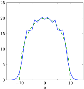
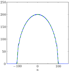
where $\lceil\nu R\rceil$ denotes the smallest integer that is greater than or equal to $\nu R$. This can also be seen in figure 3.1, where we include plots of $s_{n}^{2}(R)$ (solid line) together with plots of the asymptote $2\sqrt{R^{2}-n^{2}}$ (dashed line) for $R=10$ (left) and $R=100$ (right).

Figure 3.1: Squared singular values $s_{n}^{2}(R)$ (solid line) and asymptote $2\sqrt{R^{2}-n^{2}}$ (dashed line) for $R=10$ (left) and $R=100$ (right).

The asymptotic regime in (3.9) is already reached for moderate values of $R$.

The forgoing yields a very explicit understanding of the restricted Fourier transform $\mathcal{F}_{B_{R}(0)}$. For $|n|\lesssim R$ the singular values $s_{n}(R)$ are uniformly large, while for $|n|\gtrsim R$ the $s_{n}(R)$ are close to zero, and it is seen from (3.7)–(3.9) as well as from figure 3.1 that as $R$ gets large the width of the $n$-interval in which $s_{n}(R)$ falls from uniformly large to zero decreases. Similar properties are known for the singular values of more classical restricted Fourier transforms (see [23]).

A physical source has limited power, which we denote by $P>0$, and a receiver has a power threshold, which we denote by $p>0$. If the radiated far field has power less than $p$, the receiver cannot detect it. Because $s_{-n}^{2}(R)=s_{n}^{2}(R)$ and the odd and even squared singular values, $s_{n}^{2}(R)$, are decreasing as functions of $n\geq 0$, we may define:

$$N(R,P,p)\,:=\,\sup_{s_{n}^{2}(R)\geq{2\pi}\frac{p}{P}}n\,.$$ (3.10)

So, if $\alpha\in L^{2}(S^{1})$ is a far field radiated by a limited power source supported in $B_{R}(0)$ with ${\|f_{\alpha}^{*}\|_{L^{2}(B_{R}(0))}^{2}\leq P}$, then, for $N=N(R,P,p)$

$$P\,\geq\,\frac{1}{2\pi}\sum_{|n|>N}\frac{|\alpha_{n}|^{2}}{s_{n}^{2}(R)}\,\geq\,\frac{1}{2\pi}\frac{1}{s_{N+1}^{2}(R)}\sum_{|n|>N}|\alpha_{n}|^{2}\,>\,\frac{P}{p}\sum_{|n|>N}|\alpha_{n}|^{2}\,.$$

Accordingly, $\sum_{|n|\geq N}|\alpha_{n}|^{2}<p$ is below the power threshold. So the subspace of detectable far fields, that can be radiated by a power limited source supported in $B_{R}(0)$ is:

$$V_{\mathrm{NE}}\,:=\,\Bigl{\{}\alpha\in L^{2}(S^{1})\;\Big{|}\;\alpha(\theta)=\sum_{n=-N}^{N}\alpha_{n}e^{in\theta}\Bigr{\}}\,.$$

We refer to $V_{\mathrm{NE}}$ as the subspace of non-evanescent far fields, and to the orthogonal projection of a far field onto this subspace as the non-evanescent part of the far field. We use the term non-evanescent because it is the phenomenon of evanescence that explains why the the singular values $s_{n}^{2}(R)$ decrease rapidly for $|n|\gtrsim R$, resulting in the fact that, for a wide range of $p$ and $P$, $R<N(R,p,P)<1.5R$, if $R$ is sufficiently large.

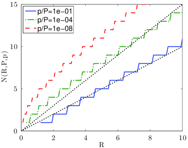
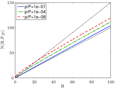
Figure 3.2: Threshold $N(R,P,p)$ as function of $R$ for different values of $p/P$. Dotted lines correspond to $g_{1}(R)=R$ and $g_{1.5}(R)=1.5R$.

This is also illustrated in figure 3.2, where we include plots of $N(R,P,p)$ from (3.10) for $p/P=10^{-1}$, $p/P=10^{-4}$, and $p/P=10^{-8}$ and for varying $R$. The dotted lines in these plots correspond to $g_{1}(R)=R$ and $g_{1.5}(R)=1.5R$, respectively.

4 Uncertainty principles for far field translation

In the inverse source problem, we seek to recover information about the size and location of the support of a source from observations of its far field. Because the far field is a restricted Fourier transform, the formula for the Fourier transform of the translation of a function:

$$\widehat{f(\cdot+c)}(\theta)\,=\,e^{\mathrm{i}c\cdot\theta}\widehat{f}(\theta)\,,\qquad\theta\in S^{1}\,,\;c\in{\mathbb{R}}^{2}\,,$$

plays an important role. We use $T_{c}$ to denote the map from ${L^{2}}(S^{1})$ to itself given by

$$T_{c}:\alpha\mapsto e^{\mathrm{i}c\cdot\theta}\alpha\,.$$ (4.1)

The mapping $T_{c}$ acts on the Fourier coefficients $\{\alpha_{n}\}$ of $\alpha$ as a convolution operator, i.e., the Fourier coefficients $\{\alpha_{m}^{c}\}$ of $T_{c}\alpha$ satisfy

$$\alpha^{c}_{m}\,=\,\sum_{n=-\infty}^{\infty}\alpha_{m-n}\bigl{(}\mathrm{i}^{n}J_{n}(|c|)e^{\mathrm{i}n\varphi_{c}}\bigr{)}\,,\qquad m\in{\mathbb{Z}}\,,$$ (4.2)

where $|c|$ and $\varphi_{c}$ are the polar coordinates of $c$. Employing a slight abuse of notation, we also use $T_{c}$ to denote the corresponding operator from ${l^{2}}$ to itself that maps

$$T_{c}:\{\alpha_{n}\}\mapsto\{\alpha^{c}_{m}\}\,.$$ (4.3)

Note that $T_{c}$ is a unitary operator on ${l^{2}}$, i.e. $T_{c}^{*}=T_{-c}$.

The following theorem, which we call an uncertainty principle for the translation operator, will be the main ingredient in our analysis of far field splitting.

Theorem 4.1 (Uncertainty principle for far field translation).

Let $\alpha,\beta\in{L^{2}}(S^{1})$ such that the corresponding Fourier coefficients $\{\alpha_{n}\}$ and $\{\beta_{n}\}$ satisfy $\operatorname{supp}\{\alpha_{n}\}\subseteq W_{1}$ and $\operatorname{supp}\{\beta_{n}\}\subseteq W_{2}$ with $W_{1},W_{2}\subseteq{\mathbb{Z}}$, and let $c\in{\mathbb{R}}^{2}$. Then,

$$|\langle\alpha,T_{c}\beta\rangle_{L^{2}(S^{1})}|\,\leq\,\frac{\sqrt{|W_{1}||W_{2}|}}{|c|^{1/3}}\|\alpha\|_{L^{2}(S^{1})}\|\beta\|_{L^{2}(S^{1})}\,.$$

We will frequently be discussing properties of a far field $\alpha$ and those of its Fourier coefficients. The following notation will be a useful shorthand:

$$\|\alpha\|_{L^{p}} \,=\,\Bigl{(}\int_{S^{1}}|\alpha(\theta)|^{p}\,\operatorname{d\!}\theta\Bigr{)}^{1/p}\,, 1\leq p\leq\infty\,,$$ (4.4)

$$\|\alpha\|_{l^{p}} \,=\,\Bigl{(}\sum_{n=-\infty}^{\infty}|\alpha_{n}|^{p}\Bigr{)}^{1/p}\,, 1\leq p\leq\infty\,.$$ (4.5)

The notation emphasizes that we treat the representation of the function $\alpha$ by its values, or by the sequence of its Fourier coefficients as simply a way of inducing different norms. That is, both (4.4) and (4.5) describe different norms of the same function on $S^{1}$. Note that, because of the Plancherel equality (3.5), $\|\alpha\|_{{L^{2}}}=\|\alpha\|_{{l^{2}}}$, so we may just write $\|\alpha\|_{2}$, and we write $\langle\cdot,\cdot\rangle$ for the corresponding inner product.

Remark 4.2.

We will extend the notation a little more and refer to the support of $\alpha$ in $S^{1}$ as its ${L^{0}}$-support and denote by $\|\alpha\|_{{L^{0}}}$ the measure of $\operatorname{supp}(\alpha)\subseteq S^{1}$. We will call the indices of the nonzero Fourier coefficients in its Fourier series expansion the ${l^{0}}$-support of $\alpha$, and use $\|\alpha\|_{l^{0}}$ to denote the number of non-zero coefficients. $\lozenge$

With this notation, theorem 4.1 becomes

Theorem 4.3 (Uncertainty principle for far field translation).

Let $\alpha,\beta\in{L^{2}}(S^{1})$, and let $c\in{\mathbb{R}}^{2}$. Then,

$$|\langle\alpha,T_{c}\beta\rangle|\,\leq\,\frac{\sqrt{\|\alpha\|_{l_{0}}\|\beta\|_{l_{0}}}}{|c|^{1/3}}\|\alpha\|_{2}\|\beta\|_{2}\,.$$ (4.6)

We refer to theorem 4.3 as an uncertainty principle, because, if we could take $\beta=T_{c}^{*}\alpha$ in (4.6), it would yield

$$1\,\leq\,\frac{\|\alpha\|_{{l^{0}}}\|T_{c}^{*}\alpha\|_{{l^{0}}}}{|c|^{2/3}}\,.$$ (4.7)

As stated, (4.7) is is true but not useful, because $\|\alpha\|_{{l^{0}}}$ and $\|T_{c}^{*}\alpha\|_{{l^{0}}}$ cannot simultaneously be finite. We present the corollary only to illustrate the close analogy to the theorem 1 in [7], which treats the discrete Fourier transform (DFT) on sequences of length $N$:

Theorem 4.4 (Uncertainty principle for the Fourier transform (Donoho, Stark [7])).

If $x$ represents the sequence $\{x_{n}\}$ for $n=0,\ldots,N-1$ and $\widehat{x}$ its DFT, then

$$1\,\leq\,\frac{\|x\|_{{l^{0}}}\|\widehat{x}\|_{{l^{0}}}}{N}\,.$$

This is a lower bound on the time-bandwidth product. In [7] Donoho and Stark present two important corollaries of uncertainty principles for the Fourier transform. One is the uniqueness of sparse representations of a signal $x$ as a superposition of vectors taken from both the standard basis and the basis of Fourier modes, and the second is the recovery of this representation by ${l^{1}}$ minimization.

The main observation we make here is that, if we phrase our uncertainty principle as in theorem 4.3, then the far field translation operator, as well as the map from $\alpha$ to its Fourier coefficients, satisfy an uncertainty principle. Combining the uncertainty principle with the regularized Picard criterion from section 3 yields analogs of both results in the context of the inverse source problem. These include previous results about the splitting of far fields from [9] and [10], which can be simplified and extended by viewing them as consequences of the uncertainty principle and the regularized Picard criterion.

The proof of theorem 4.3 is a simple corollary of the lemma below:

Lemma 4.5.

Let $c\in{\mathbb{R}}^{2}$ and let $T_{c}$ be the operator introduced in (4.1) and (4.3). Then, the operator norm of $T_{c}:\,L^{p}(S^{1})\longrightarrow L^{p}(S^{1})$, $1\leq p\leq\infty$, satisfies

$$\|T_{c}\|_{{L^{p}},{L^{p}}}\,=\,1\,,$$ (4.8)

whereas $T_{c}:{l^{1}}\longrightarrow{l^{\infty}}$ fulfills

$$\|T_{c}\|_{{l^{1}},{l^{\infty}}}\,\leq\,\frac{1}{|c|^{\frac{1}{3}}}\,.$$ (4.9)

Proof.

Recalling (4.1), we see that $T_{c}$ is multiplication by a function of modulus one, so (4.8) is immediate. On the other hand, combining (4.2) with the last inequality from page 199 of [20]; more precisely,

$$|J_{n}(x)|\,<\,\frac{b}{|x|^{\frac{1}{3}}}\qquad\text{with }b\approx 0.6749\,,$$

shows that

$$\|T_{c}\|_{{l^{1}},{l^{\infty}}}\,\leq\,\sup_{n\in{\mathbb{Z}}}|J_{n}(|c|)|\,\leq\,\frac{1}{|c|^{\frac{1}{3}}}\,.$$

∎

Proof of theorem 4.3.

Using Hölder’s inequality and (4.9) we obtain that

$$|\langle\alpha,T_{c}\beta\rangle|\,\leq\,\|\alpha\|_{{l^{1}}}\|T_{c}\beta\|_{{l^{\infty}}}\,\leq\,\frac{1}{|c|^{\frac{1}{3}}}\|\alpha\|_{{l^{1}}}\;\|\beta\|_{{l^{1}}}\,\leq\,\frac{\sqrt{\|\alpha\|_{{l^{0}}}\|\beta\|_{{l^{0}}}}}{|c|^{\frac{1}{3}}}\|\alpha\|_{{l^{2}}}\|\beta\|_{{l^{2}}}\,.$$

∎

We can improve the dependence on $|c|$ in (4.6) under hypotheses on $\alpha$ and $\beta$ that are more restrictive, but well suited to the inverse source problem.

Theorem 4.6.

Suppose that $\alpha\in{l^{2}}(-M,M)$, $\beta\in{l^{2}}(-N,N)$ with $M,N\geq 1$, and let $c\in{\mathbb{R}}^{2}$ such that $|c|>2(M+N+1)$. Then

$$|\langle\alpha,T_{c}\beta\rangle|\,\leq\,\frac{\sqrt{(2N+1)(2M+1)}}{|c|^{\frac{1}{2}}}\|\alpha\|_{2}\|\beta\|_{2}\,.$$ (4.10)

Proof.

Because the ${l^{0}}$-support of $\beta$ is contained in $[-N,N]$

$$\beta^{c}_{m}\,=\,\sum_{n=-N}^{N}\beta_{n}\Bigl{(}\mathrm{i}^{m-n}J_{m-n}(|c|)e^{\mathrm{i}(m-n)\varphi_{c}}\Bigr{)}$$

so

$$\sup_{-M<m<M}|\beta^{c}_{m}|\,\leq\,\|\beta\|_{{l^{1}}}\sup_{-(M+N)<n<(M+N)}|J_{n}(|c|)|$$

and it follows from theorem 2 of [16], using the fact that $M,N\geq 1$, together with our hypothesis, which implies that $|c|>6$, that

$$\sup_{-(M+N)<n<(M+N)}J_{n}^{2}(|c|)\,\leq\,\frac{b}{|c|}\qquad\text{with $b\approx 0.7595$}$$ (4.11)

(see appendix B for details). We now simply repeat the proof of theorem 4.3, replacing the estimate for $\|T_{c}\beta\|_{{l^{\infty}}}$ from (4.9) with the estimate we have just established in (4.11), i.e.

$$\|T_{c}\|_{{l^{1}}[-N,N],{l^{\infty}}[-M,M]}\,\leq\,\frac{1}{|c|^{\frac{1}{2}}}\,.$$ (4.12)

∎

We will also make use of another uncertainty principle. A glance at (3.4)–(3.5) reveals that the operator which maps $\alpha$ to its Fourier coefficients maps ${L^{2}}$ to ${l^{2}}$ with norm 1, ${L^{1}}$ to ${l^{\infty}}$ with norm $1/\sqrt{2\pi}$, and its inverse maps ${l^{1}}$ to ${L^{\infty}}$, also with norm $1/\sqrt{2\pi}$. An immediate corollary of this observation is

Theorem 4.7.

Let $\alpha,\beta\in L^{2}(S^{1})$ and let $c\in{\mathbb{R}}^{2}$. Then,

$$|\langle T_{c}\alpha,\beta\rangle|\,\leq\,\sqrt{\frac{\|\alpha\|_{{l^{0}}}\|\beta\|_{{L^{0}}}}{2\pi}}\|\alpha\|_{2}\|\beta\|_{2}\,.$$ (4.13)

Proof.

Combining Hölder’s inequality with (4.8) and using the mapping properties of the operator which maps $\alpha$ to its Fourier coefficients we find that

$$\begin{split}|\langle T_{c}\alpha,\beta\rangle|&\,\leq\,\|T_{c}\alpha\|_{{L^{\infty}}}\|\beta\|_{{L^{1}}}\,\leq\,\|\alpha\|_{{L^{\infty}}}\|\beta\|_{{L^{1}}}\,\leq\,\frac{1}{\sqrt{2\pi}}\|\alpha\|_{{l^{1}}}\|\beta\|_{{L^{1}}}\\ &\,\leq\,\frac{1}{\sqrt{2\pi}}\sqrt{\|\alpha\|_{{l^{0}}}}\|\alpha\|_{2}\sqrt{\|\beta\|_{{L^{0}}}}\|\beta\|_{2}\,.\end{split}$$

∎

5 ${l^{2}}$ corollaries of the uncertainty principles

The regularized Picard criterion tells us that, up to an ${L^{2}}$-small error, a far field radiated by a limited power source in $B_{R}(0)$ is ${L^{2}}$-close to an $\alpha$ that belongs to the subspace of non-evanescent far fields, the span of $\{e^{\mathrm{i}n\theta}\}$ with $|n|\leq N$, where $N=N(R,P,p)$ is a little bigger than the radius $R$. This non-evanescent $\alpha$ satisfies $\|\alpha\|_{{l^{0}}}\leq 2N+1$. The uncertainty principle will show that the angle between translates of these subspaces is bounded below when the translation parameter is large enough, so that we can split the sum of the two non-evanescent far fields into the original two summands.

Lemma 5.1.

Suppose that $\gamma,\alpha_{1},\alpha_{2}\in{L^{2}}(S^{1})$ and $c_{1},c_{2}\in{\mathbb{R}}^{2}$ with

$$\gamma\,=\,T^{*}_{c_{1}}\alpha_{1}+T^{*}_{c_{2}}\alpha_{2}$$ (5.1)

and that $\frac{\|\alpha_{1}\|_{{l^{0}}}\|\alpha_{2}\|_{{l^{0}}}}{|c_{1}-c_{2}|^{\frac{2}{3}}}<1$. Then, for $i=1,2$

$$\|\alpha_{i}\|_{2}^{2}\,\leq\,\biggl{(}1-\frac{\|\alpha_{1}\|_{{l^{0}}}\|\alpha_{2}\|_{{l^{0}}}}{|c_{1}-c_{2}|^{\frac{2}{3}}}\biggr{)}^{-1}\|\gamma\|_{2}^{2}\,.$$ (5.2)

Proof.

We first note that (5.1) and (4.1) imply

$$\begin{split}\|\gamma\|_{2}^{2}&\,\geq\,\|\alpha_{1}\|_{2}^{2}+\|\alpha_{2}\|_{2}^{2}-2|\langle T^{*}_{c_{1}}\alpha_{1},T^{*}_{c_{2}}\alpha_{2}\rangle|\\ &\,=\,\|\alpha_{1}\|_{2}^{2}+\|\alpha_{2}\|_{2}^{2}-2|\langle\alpha_{1},T^{*}_{c_{2}-c_{1}}\alpha_{2}\rangle|\,.\end{split}$$ (5.3)

We now use (4.6),

$$\begin{split}\|\gamma\|_{2}^{2}&\,\geq\,\|\alpha_{1}\|_{2}^{2}+\|\alpha_{2}\|_{2}^{2}-2\frac{\sqrt{\|\alpha_{1}\|_{{l^{0}}}\|\alpha_{2}\|_{{l^{0}}}}}{|c_{2}-c_{1}|^{\frac{1}{3}}}\|\alpha_{1}\|_{2}\|\alpha_{2}\|_{2}\\ &\,=\,\biggl{(}1-\frac{\|\alpha_{1}\|_{{l^{0}}}\|\alpha_{2}\|_{{l^{0}}}}{|c_{2}-c_{1}|^{\frac{2}{3}}}\|\biggr{)}\|\alpha_{1}\|_{2}^{2}+\biggl{(}\|\alpha_{2}\|_{2}-\frac{\sqrt{\|\alpha_{1}\|_{{l^{0}}}\|\alpha_{2}\|_{{l^{0}}}}}{|c_{2}-c_{1}|^{\frac{1}{3}}}\|\alpha_{1}\|_{2}\biggr{)}^{2}\,.\end{split}$$ (5.4)

Dropping the second term now gives (5.2) for $\alpha_{1}$, and we may interchange the roles $\alpha_{1}$ and $\alpha_{2}$ in the proof to obtain the estimate for $\alpha_{2}$ . ∎

The analogous consequence of theorem 4.6 is

Lemma 5.2.

Suppose that $\gamma\in{L^{2}}(S^{1})$, $\alpha_{i}\in{l^{2}}(-N_{i},N_{i})$ for some $N_{i}\in{\mathbb{N}}$, $i=1,2$, and $c_{1},c_{2}\in{\mathbb{R}}^{2}$ with $|c_{1}-c_{2}|>2(N_{1}+N_{2}+1)$ and

$$\gamma\,=\,T^{*}_{c_{1}}\alpha_{1}+T^{*}_{c_{2}}\alpha_{2}\,,$$

and that $\frac{(2N_{1}+1)(2N_{2}+1)}{|c_{1}-c_{2}|}<1$. Then, for $i=1,2$

$$\|\alpha_{i}\|_{2}^{2}\,\leq\,\biggl{(}1-\frac{(2N_{1}+1)(2N_{2}+1)}{|c_{1}-c_{2}|}\biggr{)}^{-1}\|\gamma\|_{2}^{2}\,.$$ (5.5)

In our application to the inverse source problem, we will know that each far field is the translation of a far field $\alpha_{i}$, radiated by a limited power source supported in a ball centered at the origin, and therefore that all but a very small amount of the radiated power is contained in the non-evanescent part, the translation of the Fourier modes $e^{\mathrm{i}n\theta}$ for $|n|<N(R,p,P)$. The estimate in the theorem below says that, if the distances between the balls is large enough, we may uniquely solve for the non-evanescent parts of the individual far fields, and that this split is stable with respect to perturbations in the data.

Theorem 5.3.

Suppose that $\gamma^{0},\gamma^{1}\in{L^{2}}(S^{1})$, $c_{1},c_{2}\in{\mathbb{R}}^{2}$ and $N_{1},N_{2}\in{\mathbb{N}}$ such that $|c_{1}-c_{2}|>2(N_{1}+N_{2}+1)$ and

$$\frac{(2N_{1}+1)(2N_{2}+1)}{|c_{1}-c_{2}|}\,<\,1\,,$$ (5.6)

and let

$$\gamma^{0} \,\mathop{=}\limits^{\mathrm{LS}}\,T^{*}_{c_{1}}\alpha_{1}^{0}+T^{*}_{c_{2}}\alpha_{2}^{0}\,, \alpha_{i}^{0}\in{l^{2}}(-N_{i},N_{i})\,,$$ (5.7a)

$$\gamma^{1} \,\mathop{=}\limits^{\mathrm{LS}}\,T^{*}_{c_{1}}\alpha_{1}^{1}+T^{*}_{c_{2}}\alpha_{2}^{1}\,, \alpha_{i}^{1}\in{l^{2}}(-N_{i},N_{i})\,.$$ (5.7b)

Then, for $i=1,2$

$$\|\alpha^{1}_{i}-\alpha_{i}^{0}\|_{2}^{2}\,\leq\,\biggl{(}1-\frac{(2N_{1}+1)(2N_{2}+1)}{|c_{1}-c_{2}|}\biggr{)}^{-1}\|\gamma^{1}-\gamma^{0}\|_{2}^{2}\,.$$ (5.8)

The notation in (5.7) above means that the $\alpha_{i}^{j}$ are the (necessarily unique) least squares solutions to the equations $\gamma^{j}=T^{*}_{c_{1}}\alpha_{1}^{j}+T^{*}_{c_{2}}\alpha_{2}^{j}$. Recall that the far fields radiated by a limited power source from a ball have almost all, but not all, of their power (${L^{2}}$-norm) concentrated in the Fourier modes with $n\leq N(R,P,p)$. Therefore the $\gamma^{i}$ will typically not belong to the subspace that is the direct sum of $T^{*}_{c_{1}}{l^{2}}(-N_{1},N_{1})\oplus T^{*}_{c_{2}}{l^{2}}(-N_{2},N_{2})$, and therefore $\alpha_{1}^{j}$ and $\alpha_{2}^{j}$ will usually not solve equations (5.7) exactly. The estimate in (5.8) is nevertheless always true, and guarantees that the pair $(\alpha_{1}^{j},\alpha_{2}^{j})$ is unique and that the absolute condition number of the splitting operator which maps $\gamma$ to $(\alpha_{1}^{j},\alpha_{2}^{j})$ is no larger than $\left(1-\frac{(2N_{1}+1)(2N_{2}+1)}{|c_{1}-c_{2}|}\right)^{-\frac{1}{2}}$.

Proof of theorem 5.3.

Each $\gamma^{j}$ can be uniquely decomposed as

$$\gamma^{j}\,=\,w^{j}+w^{j}_{\perp}\,,$$ (5.9)

where each $w^{j}$ belongs to the $2N_{1}+2N_{2}+2$-dimensional subspace

$$W\,=\,T^{*}_{c_{1}}{l^{2}}(-N_{1},N_{1})\oplus T^{*}_{c_{2}}{l^{2}}(-N_{2},N_{2})$$

and each $w^{j}_{\perp}$ is orthogonal to $W$. The definition of least squares solutions means that

$$w^{j}\,=\,T^{*}_{c_{1}}\alpha^{j}_{1}+T^{*}_{c_{2}}\alpha^{j}_{2}\,.$$

Subtracting gives

$$w^{1}-w^{0}\,=\,T^{*}_{c_{1}}(\alpha^{1}_{1}-\alpha^{0}_{1})+T^{*}_{c_{2}}(\alpha^{1}_{2}-\alpha^{0}_{2})$$ (5.10)

and applying the estimate (5.5) yields

$$\|\alpha^{1}_{i}-\alpha^{0}_{i}\|_{2}^{2}\,\leq\,\biggl{(}1-\frac{(2N_{1}+1)(2N_{2}+1)}{|c_{1}-c_{2}|}\biggr{)}^{-1}\|w^{1}-w^{0}\|_{2}^{2}\,.$$ (5.11)

Finally, we note that

$$\|\gamma^{1}-\gamma^{0}\|_{2}^{2}\,=\,\|w^{1}-w^{0}\|_{2}^{2}+\|w^{1}_{\perp}-w^{0}_{\perp}\|_{2}^{2}\,\geq\,\|w^{1}-w^{0}\|_{2}^{2}\,,$$ (5.12)

which finishes the proof. ∎

We also have corresponding corollaries of theorem 4.7, which tell us that, if a far field is radiated from a small ball, and measured on most of the circle, then it is possible to recover its non-evanescent part on the entire circle. Theorem 5.5 below, describes the case where we cannot measure the far field $\alpha=T_{c}^{*}\alpha^{0}$ on a subset $\Omega\subseteq S^{1}$. We measure $\gamma=\alpha+\beta$, where $\beta=-\alpha\big{|}_{\Omega}$. The estimates (5.14) imply that we can stably recover the non-evanescent part of the far field on $\Omega$.

Before we state the theorem, we give the corresponding analogue of lemma 5.1 and lemma 5.2.

Lemma 5.4.

Suppose that $\gamma,\alpha,\beta\in{L^{2}}(S^{1})$ and $c\in{\mathbb{R}}^{2}$ with

$$\gamma\,=\,\beta+T^{*}_{c}\alpha$$

and that $\frac{\|\alpha\|_{{l^{0}}}\|\beta\|_{{L^{0}}}}{2\pi}<1$. Then

$$\|\alpha\|_{2}^{2} \,\leq\,\biggl{(}1-\frac{\|\alpha\|_{{l^{0}}}\|\beta\|_{{L^{0}}}}{2\pi}\biggr{)}^{-1}\|\gamma\|_{2}^{2}$$ (5.13a)

$$\|\beta\|_{2}^{2} \,\leq\,\biggl{(}1-\frac{\|\alpha\|_{{l^{0}}}\|\beta\|_{{L^{0}}}}{2\pi}\biggr{)}^{-1}\|\gamma\|_{2}^{2}\,.$$ (5.13b)

Proof.

Proceeding as in (5.3)–(5.4), but replacing (4.6) by (4.13) yields the result. ∎

Theorem 5.5.

Suppose that $\gamma^{0},\gamma^{1}\in{L^{2}}(S^{1})$, $c\in{\mathbb{R}}^{2}$, $N\in{\mathbb{N}}$ and $\Omega\subseteq S^{1}$ such that $\frac{(2N+1)|\Omega|}{2\pi}<1$, and let

$$\gamma^{0} \,\mathop{=}\limits^{\mathrm{LS}}\,\beta^{0}+T_{c}\alpha^{0}\,, \alpha^{0}\in{l^{2}}(-N,N)\text{ and }\beta^{0}\in{L^{2}}(\Omega)\,,$$

$$\gamma^{1} \,\mathop{=}\limits^{\mathrm{LS}}\,\beta^{1}+T_{c}\alpha^{1}\,, \alpha^{1}\in{l^{2}}(-N,N)\text{ and }\beta^{1}\in{L^{2}}(\Omega)\,.$$

Then

$$\|\alpha^{1}-\alpha^{0}\|_{2}^{2} \,\leq\,\biggl{(}1-\frac{(2N+1)|\Omega|}{2\pi}\biggr{)}^{-1}\|\gamma^{1}-\gamma^{0}\|_{2}^{2}$$ (5.14a)

$$\|\beta^{1}-\beta^{0}\|_{2}^{2} \,\leq\,\biggl{(}1-\frac{(2N+1)|\Omega|}{2\pi}\biggr{)}^{-1}\|\gamma^{1}-\gamma^{0}\|_{2}^{2}\,.$$ (5.14b)

Proof.

Just as in (5.9), we decompose each $\gamma^{j}$

$$\gamma^{j}\,=\,w^{j}+w^{j}_{\perp}\,,$$

where each $w^{j}$ belongs to the subspace

$$W\,=\,{L^{2}}(\Omega)\oplus T_{c}{l^{2}}(-N,N)$$

and each $w^{j}_{\perp}$ is orthogonal to $W$. Proceeding as in (5.10)–(5.11), but using the estimates from (5.13), we find

$$\|\alpha^{1}-\alpha^{0}\|_{2}^{2}\,\leq\,\biggl{(}1-\frac{(2N+1)|\Omega|}{2\pi}\biggr{)}^{-1}\|w^{1}-w^{0}\|_{2}^{2}$$

$$\|\beta^{1}-\beta^{0}\|_{2}^{2}\,\leq\,\biggl{(}1-\frac{(2N+1)|\Omega|}{2\pi}\biggr{)}^{-1}\|w^{1}-w^{0}\|_{2}^{2}$$

and then note that (5.12) is true here as well to finish the proof. ∎

A version of theorem 5.3 with multiple well-separated components is also true.

Theorem 5.6.

Suppose that $\gamma^{0},\gamma^{1}\in{L^{2}}(S^{1})$, $c_{i}\in{\mathbb{R}}^{2}$ and $N_{i}\in{\mathbb{N}}$, $i=1,\ldots,I$, such that $|c_{i}-c_{j}|>2(N_{i}+N_{j}+1)$ for every $i\neq j$ and

$$\biggl{(}\sqrt{2N_{i}+1}\sum_{j\not=i}\sqrt{\frac{2N_{j}+1}{|c_{i}-c_{j}|}}\biggr{)}\,<\,1\qquad\text{for each }i\,,$$

and let

$$\gamma^{0} \,\mathop{=}\limits^{LS}\,\sum_{i=1}^{I}T^{*}_{c_{i}}\alpha_{i}^{0}\,, \alpha_{i}^{0}\in{l^{2}}(-N_{i},N_{i})\,,$$

$$\gamma^{1} \,\mathop{=}\limits^{LS}\,\sum_{i=1}^{I}T^{*}_{c_{i}}\alpha_{i}^{1}\,, \alpha_{i}^{1}\in{l^{2}}(-N_{i},N_{i})\,.$$

Then, for $i=1,\ldots,I$

$$\|\alpha_{i}^{1}-\alpha_{i}^{0}\|_{2}^{2}\,\leq\,\biggl{(}1-\sqrt{2N_{i}+1}\sum_{j\not=i}\sqrt{\frac{2N_{j}+1}{|c_{j}-c_{i}|}}\biggr{)}^{-1}\|\gamma^{1}-\gamma^{0}\|_{2}^{2}\,.$$

Proof.

As in (5.9), we decompose each $\gamma^{j}$

$$\gamma^{j}\,=\,w^{j}+w^{j}_{\perp}\,,$$

where each $w^{j}$ belongs to the subspace

$$W\,=\,\bigoplus_{i=1}^{I}T^{*}_{c_{i}}{l^{2}}(-N_{i},N_{i})$$

and each $w^{j}_{\perp}$ is orthogonal to $W$. Subtracting gives

$$w^{1}-w^{0}\,=\,\sum_{i=1}^{I}T^{*}_{c_{i}}(\alpha_{i}^{1}-\alpha_{i}^{0})$$

and applying (4.10) shows that

$$\begin{split}\|w^{1}-w^{0}\|_{2}^{2}&\,\geq\,\sum_{i=1}^{I}\|\alpha_{i}^{1}-\alpha_{i}^{0}\|_{2}^{2}-\sum_{i=1}^{I}\sum_{j\not=i}|\langle\alpha_{i}^{1}-\alpha_{i}^{0},T^{*}_{c_{j}-c_{i}}(\alpha_{j}^{1}-\alpha_{j}^{0})\rangle|\\ &\,\geq\,\sum_{i=1}^{I}\|\alpha_{i}^{1}-\alpha_{i}^{0}\|_{2}^{2}-\sum_{i=1}^{I}\sum_{j\not=i}\biggl{(}\Bigl{(}\frac{r_{i}r_{j}}{|c_{ij}|}\Bigr{)}^{\frac{1}{4}}\|\alpha_{i}^{1}-\alpha_{i}^{0}\|_{2}\Bigl{(}\frac{r_{i}r_{j}}{|c_{ij}|}\Bigr{)}^{\frac{1}{4}}\|\alpha_{j}^{1}-\alpha_{j}^{0}\|_{2}\biggr{)}\\ &\,\geq\,\sum_{i=1}^{I}\|\alpha_{i}^{1}-\alpha_{i}^{0}\|_{2}^{2}-\frac{1}{2}\biggl{(}\sum_{i=1}^{I}\sum_{j\not=i}\biggl{(}\Bigl{(}\frac{r_{i}r_{j}}{|c_{ij}|}\Bigr{)}^{\frac{1}{2}}\|\alpha_{i}^{1}-\alpha_{i}^{0}\|_{2}^{2}+\Bigl{(}\frac{r_{i}r_{j}}{|c_{ij}|}\Bigr{)}^{\frac{1}{2}}\|\alpha_{j}^{1}-\alpha_{j}^{0}\|_{2}^{2}\biggr{)}\\ &\,=\,\sum_{i=1}^{I}\|\alpha_{i}^{1}-\alpha_{i}^{0}\|_{2}^{2}\biggl{(}1-\sum_{j\not=i}\Bigl{(}\frac{r_{i}r_{j}}{|c_{ij}|}\Bigr{)}^{\frac{1}{2}}\biggr{)}\,,\end{split}$$ (5.15)

where $r_{i}=2N_{i}+1$, $r_{j}=2N_{j}+1$ and $c_{ij}=c_{i}-c_{j}$. Since (5.12) is true here as well this ends the proof. ∎

We may include a missing data component as well.

Theorem 5.7.

Suppose that $\gamma^{0},\gamma^{1}\in{L^{2}}(S^{1})$, $c_{i}\in{\mathbb{R}}^{2}$, $N_{i}\in{\mathbb{N}}$, $i=1,\ldots,I$, and $\Omega\subseteq{L^{2}}(S^{1})$ such that $|c_{i}-c_{j}|>2(N_{i}+N_{j}+1)$ for every $i\neq j$ and

$$\sqrt{\frac{|\Omega|}{2\pi}}\sum_{i=1}^{I}\sqrt{2N_{i}+1} \,<\,1\,,$$

$$\sqrt{2N_{i}+1}\biggl{(}\sqrt{\frac{|\Omega|}{2\pi}}+\sum_{j\neq i}\sqrt{\frac{2N_{i}+1}{|c_{i}-c_{j}|}}\biggr{)} \,<\,1\qquad\text{for each }i\,,$$

and let

$$\gamma^{0} \,\mathop{=}\limits^{LS}\,\beta^{0}+\sum_{i=1}^{I}T^{*}_{c_{i}}\alpha_{i}^{0}\,, \alpha_{i}^{0}\in{l^{2}}(-N_{i},N_{i})\text{ and }\beta^{0}\in{L^{2}}(\Omega)\,,$$ (5.16a)

$$\gamma^{1} \,\mathop{=}\limits^{LS}\,\beta^{1}+\sum_{i=1}^{I}T^{*}_{c_{i}}\alpha_{i}^{1}\,, \alpha_{i}^{1}\in{l^{2}}(-N_{i},N_{i})\text{ and }\beta^{0}\in{L^{2}}(\Omega)\,.$$ (5.16b)

Then

$$\|\beta^{1}-\beta^{0}\|_{2}^{2} \,\leq\,\biggl{(}1-\sqrt{\frac{|\Omega|}{2\pi}}\sum_{i}\sqrt{2N_{i}+1}\biggr{)}^{-1}\|\gamma^{1}-\gamma^{0}\|_{2}^{2}$$

and, for $$i=1,\ldots,I$$

$$\|\alpha_{i}^{1}-\alpha_{i}^{0}\|_{2}^{2} \,\leq\,\biggl{(}1-\sqrt{2N_{i}+1}\biggl{(}\sqrt{\frac{|\Omega|}{2\pi}}+\sum_{j\neq i}\sqrt{\frac{2N_{i}+1}{|c_{i}-c_{j}|}}\biggr{)}\biggr{)}^{-1}\|\gamma^{1}-\gamma^{0}\|_{2}^{2}\,.$$

Proof.

As in (5.9), we decompose each $\gamma^{j}$

$$\gamma^{j}\,=\,w^{j}+w^{j}_{\perp}\,,$$

where each $w^{j}$ belongs to the subspace

$$W\,=\,L^{2}(\Omega)\oplus\bigoplus_{i=1}^{J}T^{*}_{c_{i}}{l^{2}}(-N_{i},N_{i})$$

and each $w^{j}_{\perp}$ is orthogonal to $W$. Subtracting gives

$$w^{1}-w^{0}\,=\,\beta^{1}-\beta^{0}+\sum_{i=1}^{I}T^{*}_{c_{i}}(\alpha_{i}^{1}-\alpha_{i}^{0})$$

and thus

$$\begin{split}\|w^{1}-w^{0}\|_{2}^{2}&\,\geq\,\|\beta^{1}-\beta^{0}\|_{2}^{2}-2\sum_{i=1}^{I}|\langle T^{*}_{c_{i}}(\alpha_{i}^{1}-\alpha_{i}^{0}),\beta^{1}-\beta^{0}\rangle|\\ &\phantom{\,\geq\,}+\sum_{i=1}^{I}\|\alpha_{i}^{1}-\alpha_{i}^{0}\|_{2}^{2}-\sum_{i=1}^{I}\sum_{j\not=i}|\langle\alpha_{i}^{1}-\alpha_{i}^{0},T^{*}_{c_{j}-c_{i}}(\alpha_{j}^{1}-\alpha_{j}^{0})\rangle|\,.\end{split}$$

Proceeding as in (5.15), using (4.10) and (4.13), and applying (5.12) finishes the proof. ∎

6 ${l^{1}}$ corollaries of the uncertainty principle

The results below are analogous to those in the previous section. The main difference is that they do not require the a priori knowledge of the size of the non-evanescent subspaces (the $N_{i}$ in theorems 5.3 through 5.7).

In theorem 6.1 below, $\gamma^{0}$ represents the (measured) approximate far field; the $\alpha_{i}^{0}$ are the non-evanescent parts of the true (unknown) far fields radiated by each of the two components, which we assume are well-separated (6.1). The constant $\delta_{0}$ in (6.2) accounts for both the noise and the evanescent components of the true far fields. Condition (6.3) requires that the optimization problem (6.4) be formulated with a constraint that is weak enough so that the $\alpha_{i}^{0}$ are feasible.

Theorem 6.1.

Suppose that $\gamma^{0},\alpha_{1}^{0},\alpha_{2}^{0}\in{L^{2}}(S^{1})$ and $c_{1},c_{2}\in{\mathbb{R}}^{2}$ such that

$$\frac{4\|\alpha_{i}^{0}\|_{{l^{0}}}}{|c_{1}-c_{2}|^{\frac{1}{3}}}\,<\,1\qquad\text{for each }i$$ (6.1)

and

$$\|\gamma^{0}-T^{*}_{c_{1}}\alpha_{1}^{0}-T^{*}_{c_{2}}\alpha_{2}^{0}\|_{2}\,\leq\,\delta_{0}\qquad\text{for some }\delta_{0}\geq 0\,.$$ (6.2)

If $\delta\geq 0$ and $\gamma\in{L^{2}}(S^{1})$ with

$$\delta\,\geq\,\delta_{0}+\|\gamma-\gamma^{0}\|_{2}$$ (6.3)

and

$$(\alpha_{1},\alpha_{2})=\mathop{\mathrm{missing}}{argmin}\limits\|\alpha_{1}\|_{{l^{1}}}+\|\alpha_{2}\|_{{l^{1}}}\quad\text{s.t.}\quad{\|\gamma-T^{*}_{c_{1}}\alpha_{1}-T^{*}_{c_{2}}\alpha_{2}\|_{2}\leq\delta}\,,\;\alpha_{1},\alpha_{2}\in{L^{2}}(S^{1})\,,$$ (6.4)

then, for $i=1,2$

$$\|\alpha^{0}_{i}-\alpha_{i}\|_{2}^{2}\,\leq\,\Bigl{(}1-\frac{4\|\alpha_{i}^{0}\|_{{l^{0}}}}{|c_{1}-c_{2}|^{\frac{1}{3}}}\Bigr{)}^{-1}4\delta^{2}\,.$$ (6.5)

Proof.

A consequence of (6.3) is that the pair $(\alpha_{1}^{0},\alpha_{2}^{0})$ satisfies the constraint in (6.4), which implies that

$$\|\alpha_{1}\|_{{l^{1}}}+\|\alpha_{2}\|_{{l^{1}}}\,\leq\,\|\alpha_{1}^{0}\|_{{l^{1}}}+\|\alpha_{2}^{0}\|_{{l^{1}}}$$ (6.6)

because $(\alpha_{1},\alpha_{2})$ is a minimizer. Additionally, with $W_{i}$ representing the ${l^{0}}$-support of $\alpha^{0}_{i}$ and $W_{i}^{c}$ its complement,

$$\begin{split}\|\alpha_{i}\|_{{l^{1}}}&\,=\,\|\alpha_{i}^{0}+(\alpha_{i}-\alpha_{i}^{0})\|_{{l^{1}}}\\ &\,=\,\|\alpha_{i}^{0}+(\alpha_{i}-\alpha_{i}^{0})\|_{{l^{1}}(W_{i})}+\|\alpha_{i}-\alpha_{i}^{0}\|_{{l^{1}}(W_{i}^{c})}\\ &\,=\,\|\alpha_{i}^{0}+(\alpha_{i}-\alpha_{i}^{0})\|_{{l^{1}}(W_{i})}+\|\alpha_{i}-\alpha_{i}^{0}\|_{{l^{1}}}-\|\alpha_{i}-\alpha_{i}^{0}\|_{{l^{1}}(W_{i})}\\ &\,\geq\,\|\alpha_{i}^{0}\|_{{l^{1}}}+\|\alpha_{i}-\alpha_{i}^{0}\|_{{l^{1}}}-2\|\alpha_{i}-\alpha_{i}^{0}\|_{{l^{1}}(W_{i})}\,.\end{split}$$ (6.7)

Inserting (6.7) into (6.6) yields

$$\|\alpha_{1}-\alpha_{1}^{0}\|_{{l^{1}}}+\|\alpha_{2}-\alpha_{2}^{0}\|_{{l^{1}}}\,\leq\,2(\|\alpha_{1}-\alpha_{1}^{0}\|_{{l^{1}}(W_{1})}+\|\alpha_{2}-\alpha_{2}^{0}\|_{{l^{1}}(W_{2})})\,.$$ (6.8)

We now use (6.3) together with (6.2), the constraint in (6.4) and the fact that $T^{*}_{c_{1}-c_{2}}$ is an ${L^{2}}$-isometry to obtain

$$\begin{split}4\delta^{2}&\,\geq\,\bigl{(}\|\gamma-\gamma^{0}\|_{2}+\delta_{0}+\delta\bigl{)}^{2}\\ &\,\geq\,\bigl{(}\|\gamma-\gamma^{0}\|_{2}+\|\gamma^{0}-T^{*}_{c_{1}}\alpha_{1}^{0}-T^{*}_{c_{2}}\alpha_{2}^{0}\|_{2}+\|\gamma-T^{*}_{c_{1}}\alpha_{1}-T^{*}_{c_{2}}\alpha_{2}\|_{2}\bigl{)}^{2}\\ &\,\geq\,\|T^{*}_{c_{1}}(\alpha_{1}-\alpha_{1}^{0})+T^{*}_{c_{2}}(\alpha_{2}-\alpha_{2}^{0})\|_{2}^{2}\\ &\,=\,\|\alpha_{1}-\alpha_{1}^{0}+T^{*}_{c_{2}-c_{1}}(\alpha_{2}-\alpha_{2}^{0})\|_{2}^{2}\\ &\,\geq\,\|\alpha_{1}-\alpha_{1}^{0}\|_{2}^{2}+\|\alpha_{2}-\alpha_{2}^{0}\|_{2}^{2}-2|\langle\alpha_{1}-\alpha_{1}^{0},T^{*}_{c_{2}-c_{1}}(\alpha_{2}-\alpha_{2}^{0})\rangle|\,.\end{split}$$ (6.9)

Hölder’s inequality, (4.9), and (6.8) show

$$\begin{split}4\delta^{2}&\,\geq\,\|\alpha_{1}-\alpha_{1}^{0}\|_{2}^{2}+\|\alpha_{2}-\alpha_{2}^{0}\|_{2}^{2}-\frac{2}{|c_{1}-c_{2}|^{\frac{1}{3}}}\|\alpha_{1}-\alpha_{1}^{0}\|_{{l^{1}}}\|\alpha_{2}-\alpha_{2}^{0}\|_{{l^{1}}}\\ &\,\geq\,\|\alpha_{1}-\alpha_{1}^{0}\|_{2}^{2}+\|\alpha_{2}-\alpha_{2}^{0}\|_{2}^{2}-\frac{1}{2|c_{1}-c_{2}|^{\frac{1}{3}}}\bigl{(}\|\alpha_{1}-\alpha_{1}^{0}\|_{{l^{1}}}+\|\alpha_{2}-\alpha_{2}^{0}\|_{{l^{1}}}\bigr{)}^{2}\\ &\,\geq\,\|\alpha_{1}-\alpha_{1}^{0}\|_{2}^{2}+\|\alpha_{2}-\alpha_{2}^{0}\|_{2}^{2}-\frac{2}{|c_{1}-c_{2}|^{\frac{1}{3}}}\bigl{(}\|\alpha_{1}-\alpha_{1}^{0}\|_{{l^{1}}(W_{1})}+\|\alpha_{2}-\alpha_{2}^{0}\|_{{l^{1}}(W_{2})}\bigr{)}^{2}\,.\end{split}$$ (6.10)

Using Hölder’s inequality once more yields

$$\begin{split}4\delta^{2}&\,\geq\,\|\alpha_{1}-\alpha_{1}^{0}\|_{2}^{2}+\|\alpha_{2}-\alpha_{2}^{0}\|_{2}^{2}-\frac{2}{|c_{1}-c_{2}|^{\frac{1}{3}}}\bigl{(}|W_{1}|^{\frac{1}{2}}\|\alpha_{1}-\alpha_{1}^{0}\|_{2}+|W_{2}|^{\frac{1}{2}}\|\alpha_{2}-\alpha_{2}^{0}\|_{2}\bigr{)}^{2}\\ &\,\geq\,\|\alpha_{1}-\alpha_{1}^{0}\|_{2}^{2}+\|\alpha_{2}-\alpha_{2}^{0}\|_{2}^{2}-\frac{4}{|c_{1}-c_{2}|^{\frac{1}{3}}}\bigl{(}|W_{1}|\|\alpha_{1}-\alpha_{1}^{0}\|_{2}^{2}+|W_{2}|\|\alpha_{2}-\alpha_{2}^{0}\|_{2}^{2}\bigr{)}\,,\end{split}$$ (6.11)

which implies (6.5) because $|W_{i}|=\|\alpha_{i}^{0}\|_{{l^{0}}}$. ∎

Assuming that some a priori information on the size of the non-evanescent subspaces is available and that the distances between the source components is large relative to their dimensions, we can improve the dependence of the stability estimates on the distances.

Corollary 6.2.

If we add to the hypothesis of theorem 6.1:

$$\alpha_{i}^{0},\alpha_{i}\in{l^{2}}(-N_{i},N_{i})\qquad\text{and}\qquad|c_{1}-c_{2}|\,>\,2(N_{1}+N_{2}+1)$$

for some $N_{1},N_{2}\in{\mathbb{N}}$ and replace (6.1) with

$$\frac{4\|\alpha_{i}^{0}\|_{{l^{0}}}}{|c_{1}-c_{2}|^{\frac{1}{2}}}\,<\,1\qquad\text{for each }i$$ (6.12)

then, for $i=1,2$

$$\|\alpha^{0}_{i}-\alpha_{i}\|_{2}^{2}\,\leq\,\Bigl{(}1-\frac{4\|\alpha_{i}^{0}\|_{{l^{0}}}}{|c_{1}-c_{2}|^{\frac{1}{2}}}\Bigr{)}^{-1}4\delta^{2}\,.$$ (6.13)

Proof.

Replace (4.9) by (4.12) in (6.9)–(6.10). ∎

The constraint (6.12) in corollary 6.2 is much more restrictive than the corresponding assumption (5.6) in theorem 5.3, and also the estimate (6.13) is weaker than (5.8). However, if we add to the hypothesis of theorem 6.1 all a priori assumptions on the non-evanescent subspaces used in theorem 5.3, the result improves as follows.

Corollary 6.3.

If we add to the hypothesis of theorem 6.1:

$$\alpha_{i}^{0},\alpha_{i}\in{l^{2}}(-N_{i},N_{i})\qquad\text{and}\qquad|c_{1}-c_{2}|\,>\,2(N_{1}+N_{2}+1)$$

for some $N_{1},N_{2}\in{\mathbb{N}}$ and replace (6.1) with

$$\frac{(2N_{1}+1)(2N_{2}+1)}{|c_{1}-c_{2}|}\,<\,1$$ (6.14)

the conclusion becomes

$$\|\alpha^{0}_{i}-\alpha_{i}^{1}\|_{2}^{2}\,\leq\,\Bigl{(}1-\frac{(2N_{1}+1)(2N_{2}+1)}{|c_{1}-c_{2}|}\Bigr{)}^{-1}4\delta^{2}\,.$$ (6.15)

The constraint (6.14) in corollary 6.3 is now the same as the corresponding assumption (5.6) in theorem 5.3, but the estimate (6.15) still differs from (5.8) (after taking the square root on both sides of these inequalities) by a factor of two. However, the main advantage of the ${l^{1}}$ approach is clearly that no a priori knowledge of the size of the non-evanescent subspaces is required. If such a priori information is available, we recommend using least squares.

Proof of corollary 6.3.

Proceeding as in (6.9) and applying (4.10), we find that

$$\begin{split}4\delta^{2}&\,\geq\,\|\alpha_{1}-\alpha_{1}^{0}\|_{2}^{2}+\|\alpha_{2}-\alpha_{2}^{0}\|_{2}^{2}-2|\langle\alpha_{1}-\alpha_{1}^{0},T^{*}_{c_{2}-c_{1}}(\alpha_{2}-\alpha_{2}^{0})\rangle|\\ &\,\geq\,\|\alpha_{1}-\alpha_{1}^{0}\|_{2}^{2}+\|\alpha_{2}-\alpha_{2}^{0}\|_{2}^{2}-2\Bigl{(}\frac{r_{1}r_{2}}{|c_{12}|}\Bigr{)}^{\frac{1}{2}}\|\alpha_{1}-\alpha_{1}^{0}\|_{2}\|\alpha_{2}-\alpha_{2}^{0}\|_{2}\\ &\,\geq\,\biggl{(}1-\frac{r_{1}r_{2}}{|c_{12}|}\biggr{)}\|\alpha_{1}-\alpha_{1}^{0}\|_{2}^{2}+\Biggl{(}\|\alpha_{2}-\alpha_{2}^{0}\|_{2}-\Bigl{(}\frac{r_{1}r_{2}}{|c_{12}|}\Bigr{)}^{\frac{1}{2}}\|\alpha_{1}-\alpha_{1}^{0}\|_{2}\Biggr{)}^{2}\,,\end{split}$$

where $r_{1}=2N_{1}+1$, $r_{2}=2N_{2}+1$ and $c_{12}=c_{1}-c_{2}$. Dropping the second term gives (6.13) for $\alpha_{1}$, and we may interchange the roles of $\alpha_{1}$ and $\alpha_{2}$ in the proof to obtain the estimate for $\alpha_{2}$. ∎

The analogue of theorem 5.5 for data completion but without a priori knowledge on the size of the non-evanescent subspaces is

Theorem 6.4.

Suppose that $\gamma^{0},\alpha^{0}\in{L^{2}}(S^{1})$, $\Omega\subseteq S^{1}$, $\beta^{0}\in{L^{2}}(\Omega)$ and $c\in{\mathbb{R}}^{2}$ such that

$$\frac{2\|\alpha^{0}\|_{{l^{0}}}|\Omega|}{\pi}\,<\,1$$

and

$$\|\gamma^{0}-T^{*}_{c}\alpha^{0}-\beta^{0}\|_{2}\,\leq\,\delta_{0}\qquad\text{for some }\delta^{0}\geq 0\,.$$

If $\delta\geq 0$ and $\gamma\in{L^{2}}(S^{1})$ with

$$\delta\,\geq\,\delta_{0}+\|\gamma-\gamma^{0}\|_{2}$$

and

$$\alpha=\mathop{\mathrm{missing}}{argmin}\limits\|\alpha\|_{{l^{1}}}\quad\text{s.t.}\quad{\|\gamma-\beta-T^{*}_{c}\alpha\|_{2}\leq\delta}\,,\;\alpha\in{L^{2}}(S^{1})\,,\;\beta\in L^{2}(\Omega)\,,$$

then

$$\|\alpha^{0}-\alpha\|_{2}^{2}\,\leq\,\Bigl{(}1-\frac{2\|\alpha^{0}\|_{{l^{0}}}|\Omega|}{\pi}\Bigr{)}^{-1}4\delta^{2}$$ (6.16a)

$$\|\beta^{0}-\beta\|_{2}^{2}\,\leq\,\Bigl{(}1-\frac{2\|\alpha^{0}\|_{{l^{0}}}|\Omega|}{\pi}\Bigr{)}^{-1}4\delta^{2}\,.$$ (6.16b)

Proof.

Proceeding as in (6.6)–(6.8) we find that

$$\|\alpha-\alpha^{0}\|_{{l^{1}}}\,\leq\,2\|\alpha-\alpha^{0}\|_{{l^{1}}(W)}$$ (6.17)

with $W$ representing the ${l^{0}}$-support of $\alpha^{0}$. Applying similar arguments as in (6.9) yields

$$\begin{split}4\delta^{2}\,\geq\,\|\alpha-\alpha^{0}\|_{2}^{2}+\|\beta-\beta^{0}\|_{2}^{2}-2|\langle T^{*}_{c}(\alpha-\alpha^{0}),\beta-\beta^{0}\rangle|\,.\end{split}$$

We now use Hölder’s inequality, (4.1), the mapping properties of the operator which maps $\alpha$ to its Fourier coefficients and (6.17) to obtain

$$\begin{split}4\delta^{2}&\,\geq\,\|\alpha-\alpha^{0}\|_{2}^{2}+\|\beta-\beta^{0}\|_{2}^{2}-2\|T^{*}_{c}(\alpha-\alpha^{0})\|_{{L^{\infty}}}\|\beta-\beta^{0}\|_{{L^{1}}}\\ &\,=\,\|\alpha-\alpha^{0}\|_{2}^{2}+\|\beta-\beta^{0}\|_{2}^{2}-2\|\alpha-\alpha^{0}\|_{{L^{\infty}}}\|\beta-\beta^{0}\|_{{L^{1}}}\\ &\,\geq\,\|\alpha-\alpha^{0}\|_{2}^{2}+\|\beta-\beta^{0}\|_{2}^{2}-\frac{2}{\sqrt{2\pi}}\|\alpha-\alpha^{0}\|_{{l^{1}}}\|\beta-\beta^{0}\|_{{L^{1}}}\\ &\,\geq\,\|\alpha-\alpha^{0}\|_{2}^{2}+\|\beta-\beta^{0}\|_{2}^{2}-\frac{4}{\sqrt{2\pi}}\|\alpha-\alpha^{0}\|_{{l^{1}}(W)}\|\beta-\beta^{0}\|_{{L^{1}}}\\ &\,\geq\,\|\alpha-\alpha^{0}\|_{2}^{2}+\|\beta-\beta^{0}\|_{2}^{2}-\frac{4}{\sqrt{2\pi}}\sqrt{|W|}\|\alpha-\alpha^{0}\|_{2}\sqrt{|\Omega|}\|\beta-\beta^{0}\|_{2}\\ &\,\geq\,\Bigl{(}1-\frac{2}{\pi}|W||\Omega|\Bigr{)}\|\alpha-\alpha^{0}\|_{2}^{2}+\Bigl{(}\|\beta-\beta^{0}\|_{2}-\frac{2}{\sqrt{2\pi}}\sqrt{|W||\Omega|}\|\alpha-\alpha^{0}\|_{2}\Bigr{)}^{2}\,.\end{split}$$ (6.18)

Dropping the second term gives (6.16) for $\alpha$ because $|W|=\|\alpha^{0}\|_{{l^{0}}}$, and we may interchange the roles of $\alpha$ and $\beta$ when completing the square in the last line of (6.18) to obtain the estimate for $\beta$. ∎

If $\Omega$ is unknown as well, then theorem 6.4 can be adapted as follows.

Corollary 6.5.

Suppose that $\gamma^{0},\alpha^{0}\in{L^{2}}(S^{1})$, $\Omega\subseteq S^{1}$, $\beta^{0}\in{L^{2}}(\Omega)$ and $c\in{\mathbb{R}}^{2}$ such that

$$\frac{4}{\sqrt{2\pi}}\frac{1}{\tau^{2}}\|\alpha^{0}\|_{{l^{0}}}\,<\,1\quad\text{and}\quad\frac{4}{\sqrt{2\pi}}\tau^{2}|\Omega|\,<\,1\qquad\text{for some }\tau>0$$

and

$$\|\gamma^{0}-T^{*}_{c}\alpha^{0}-\beta^{0}\|_{2}\,\leq\,\delta_{0}\qquad\text{for some }\delta_{0}\geq 0\,.$$

If $\delta\geq 0$ and $\gamma\in{L^{2}}(S^{1})$ with

$$\delta\,\geq\,\delta_{0}+\|\gamma-\gamma^{0}\|_{2}$$

and

$$(\alpha,\beta)=\mathop{\mathrm{missing}}{argmin}\limits\frac{1}{\tau}\|\alpha\|_{{l^{1}}}+\tau\|\beta\|_{{L^{1}}}\quad\text{s.t.}\quad{\|\gamma-T^{*}_{c}\alpha-\beta\|_{2}\leq\delta}\,,\;\alpha,\beta\in{L^{2}}(S^{1})\,,$$

then

$$\|\alpha^{0}-\alpha\|_{2}^{2}\,\leq\,\Bigl{(}1-\frac{4}{\sqrt{2\pi}}\frac{1}{\tau^{2}}\|\alpha^{0}\|_{{l^{0}}}\Bigr{)}^{-1}4\delta^{2}$$

$$\|\beta^{0}-\beta\|_{2}^{2}\,\leq\,\Bigl{(}1-\frac{4}{\sqrt{2\pi}}\tau^{2}|\Omega|\Bigr{)}^{-1}4\delta^{2}\,.$$

Proof.

Proceeding as in (6.6)–(6.8) we find that

$$\frac{1}{\tau}\|\alpha-\alpha^{0}\|_{{l^{1}}}+\tau\|\beta-\beta^{0}\|_{{L^{1}}}\,\leq\,2\bigl{(}\frac{1}{\tau}\|\alpha-\alpha^{0}\|_{{l^{1}}(W)}+\tau\|\beta-\beta^{0}\|_{{L^{1}}(\Omega)}\bigr{)}$$ (6.19)

with $W$ representing the ${l^{0}}$-support of $\alpha^{0}$. Applying similar arguments as in (6.9)–(6.11) and (6.18) together with (6.19) yields

$$\begin{split}4\delta^{2}&\,\geq\,\|\alpha-\alpha^{0}\|_{2}^{2}+\|\beta-\beta^{0}\|_{2}^{2}-\frac{2}{\sqrt{2\pi}}\|\alpha-\alpha^{0}\|_{{l^{1}}}\|\beta-\beta^{0}\|_{{L^{1}}}\\ &\,\geq\,\|\alpha-\alpha^{0}\|_{2}^{2}+\|\beta-\beta^{0}\|_{2}^{2}-\frac{1}{2\sqrt{2\pi}}\Bigl{(}\frac{1}{\tau}\|\alpha-\alpha^{0}\|_{{l^{1}}}+\tau\|\beta-\beta^{0}\|_{{L^{1}}}\Bigr{)}^{2}\\ &\,\geq\,\|\alpha-\alpha^{0}\|_{2}^{2}+\|\beta-\beta^{0}\|_{2}^{2}-\frac{2}{\sqrt{2\pi}}\Bigl{(}\frac{1}{\tau}\|\alpha-\alpha^{0}\|_{{l^{1}}(W)}+\tau\|\beta-\beta^{0}\|_{{L^{1}}(\Omega)}\Bigr{)}^{2}\\ &\,\geq\,\|\alpha-\alpha^{0}\|_{2}^{2}+\|\beta-\beta^{0}\|_{2}^{2}-\frac{2}{\sqrt{2\pi}}\Bigl{(}\frac{1}{\tau}\sqrt{|W|}\|\alpha-\alpha^{0}\|_{2}+\tau\sqrt{|\Omega|}\|\beta-\beta^{0}\|_{2}\Bigr{)}^{2}\\ &\,\geq\,\|\alpha-\alpha^{0}\|_{2}^{2}+\|\beta-\beta^{0}\|_{2}^{2}-\frac{4}{\sqrt{2\pi}}\Bigl{(}\frac{1}{\tau^{2}}|W|\|\alpha-\alpha^{0}\|_{2}^{2}+\tau^{2}|\Omega|\|\beta-\beta^{0}\|_{2}^{2}\Bigr{)}\,.\end{split}$$

This ends the proof because $|W|=\|\alpha^{0}\|_{{l^{0}}}$. ∎

A possible application of corollary 6.5 is the problem of removing (high-amplitude) strongly localized noise from measured far field data. Next we consider sources supported on sets with multiple disjoint components.

Theorem 6.6.

Suppose that $\gamma^{0},\alpha_{i}^{0}\in{L^{2}}(S^{1})$ and $c_{i}\in{\mathbb{R}}^{2}$, $i=1,\ldots,I$ such that

$$\max_{j\not=k}\frac{1}{|c_{k}-c_{j}|^{\frac{1}{3}}}4(I-1)\|\alpha_{i}^{0}\|_{{l^{0}}}\,<\,1\qquad\text{for each }i$$ (6.20)

and

$$\|\gamma^{0}-\sum_{i=1}^{I}T^{*}_{c_{i}}\alpha_{i}^{0}\|_{2}\,\leq\,\delta_{0}\qquad\text{for some }\delta^{0}\geq 0\,.$$

If $\delta\geq 0$ and $\gamma\in{L^{2}}(S^{1})$ with

$$\delta\,\geq\,\delta_{0}+\|\gamma-\gamma^{0}\|_{2}$$

and

$$(\alpha_{1},\ldots,\alpha_{I})=\mathop{\mathrm{missing}}{argmin}\limits\sum_{i=1}^{I}\|\alpha_{i}\|_{{l^{1}}}\quad\text{s.t.}\quad{\|\gamma-\sum_{i=1}^{I}T^{*}_{c_{i}}\alpha_{i}\|_{2}\leq\delta}\,,\;\alpha_{i}\in{L^{2}}(S^{1})\,,$$ (6.21)

then, for $i=1,\ldots,I$

$$\|\alpha^{0}_{i}-\alpha_{i}\|_{2}^{2}\,\leq\,\Bigl{(}1-\max_{j\not=k}\frac{1}{|c_{k}-c_{j}|^{\frac{1}{3}}}4(I-1)\|\alpha_{i}^{0}\|_{{l^{0}}}\Bigr{)}^{-1}4\delta^{2}\,.$$

Proof.

Proceeding as in (6.6)–(6.8) we find that

$$\sum_{i=1}^{I}\|\alpha_{i}-\alpha_{i}^{0}\|_{l^{1}}\,\leq\,2\sum_{i=1}^{I}\|\alpha_{i}-\alpha_{i}^{0}\|_{l^{1}(W_{i})}$$ (6.22)

with $W_{i}$ representing the ${l^{0}}$-support of $\alpha_{i}^{0}$. Applying similar arguments as in (6.9)–(6.10) and using the inequality (C.3) from appendix C and (6.22) we obtain

$$\begin{split}4\delta^{2}&\,\geq\,\sum_{i=1}^{I}\|\alpha_{i}-\alpha_{i}^{0}\|^{2}_{2}-\sum_{i=1}^{I}\sum_{j\not=i}|\langle\alpha_{i}-\alpha_{i}^{0},T^{*}_{c_{j}-c_{i}}(\alpha_{j}-\alpha_{j}^{0})\rangle|\\ &\,\geq\,\sum_{i=1}^{I}\|\alpha_{i}-\alpha_{i}^{0}\|^{2}_{2}-\sum_{i=1}^{I}\sum_{j\not=i}\frac{1}{|c_{i}-c_{j}|^{\frac{1}{3}}}\|\alpha_{i}-\alpha_{i}^{0}\|_{l^{1}}\|\alpha_{j}-\alpha_{j}^{0}\|_{l^{1}}\\ &\,\geq\,\sum_{i=1}^{I}\|\alpha_{i}-\alpha_{i}^{0}\|^{2}_{2}-\max_{j\not=k}\frac{1}{|c_{j}-c_{k}|^{\frac{1}{3}}}\sum_{i=1}^{I}\sum_{j\not=i}\|\alpha_{i}-\alpha_{i}^{0}\|_{l^{1}}\|\alpha_{j}-\alpha_{j}^{0}\|_{l^{1}}\\ &\,\geq\,\sum_{i=1}^{I}\|\alpha_{i}-\alpha_{i}^{0}\|^{2}_{2}-\max_{j\not=k}\frac{1}{|c_{j}-c_{k}|^{\frac{1}{3}}}\frac{I-1}{I}\Bigl{(}\sum_{i=1}^{I}\|\alpha_{i}-\alpha_{i}^{0}\|_{l^{1}}\Bigr{)}^{2}\\ &\,\geq\,\sum_{i=1}^{I}\|\alpha_{i}-\alpha_{i}^{0}\|^{2}_{2}-\max_{j\not=k}\frac{1}{|c_{j}-c_{k}|^{\frac{1}{3}}}\frac{I-1}{I}4\Bigl{(}\sum_{i=1}^{I}\|\alpha_{i}-\alpha_{i}^{0}\|_{{l^{1}}(W_{i})}\Bigr{)}^{2}\,.\end{split}$$ (6.23)

Applying Hölder’s inequality and (C.2) yields

$$\begin{split}4\delta^{2}&\,\geq\,\sum_{i=1}^{I}\|\alpha_{i}-\alpha_{i}^{0}\|^{2}_{2}-\max_{j\not=k}\frac{1}{|c_{j}-c_{k}|^{\frac{1}{3}}}\frac{I-1}{I}4\Bigl{(}\sum_{i=1}^{I}|W_{i}|^{\frac{1}{2}}\|\alpha_{i}-\alpha_{i}^{0}\|_{2}\Bigr{)}^{2}\\ &\,\geq\,\sum_{i=1}^{I}\|\alpha_{i}-\alpha_{i}^{0}\|^{2}_{2}-\max_{j\not=k}\frac{1}{|c_{j}-c_{k}|^{\frac{1}{3}}}4(I-1)\sum_{i=1}^{I}|W_{i}|\|\alpha_{i}-\alpha_{i}^{0}\|_{2}^{2}\,,\end{split}$$ (6.24)

where $|W_{i}|=\|\alpha_{i}^{0}\|_{{l^{0}}}$. ∎

As in corollary 6.2 we can improve these estimates, under the assumption that some a priori knowledge of the size of the non-evanescent subspaces is available and that the individual source components are sufficiently far apart from each other.

Corollary 6.7.

If we add to the hypothesis of theorem 6.6:

$$\alpha_{i}^{0},\alpha_{i}\in{l^{2}}(-N_{i},N_{i})\quad\text{for each }i\qquad\text{and}\qquad|c_{i}-c_{j}|\,>\,2(N_{i}+N_{j}+1)\quad\text{for every }i\not=j$$

for some $N_{1},\ldots,N_{I}\in{\mathbb{N}}$, and replace (6.20) with

$$\max_{j\not=k}\frac{1}{|c_{k}-c_{j}|^{\frac{1}{2}}}4(I-1)\|\alpha_{i}^{0}\|_{l^{0}}\,<\,1\qquad\text{for each }i\,,$$

the conclusion becomes, for $i=1,\ldots,I$

$$\|\alpha^{0}_{i}-\alpha_{i}\|_{2}^{2}\,\leq\,\Bigl{(}1-\max_{j\not=k}\frac{1}{|c_{k}-c_{j}|^{\frac{1}{2}}}4(I-1)\|\alpha_{i}^{0}\|_{l^{0}}\Bigr{)}^{-1}4\delta^{2}\,.$$

Proof.

Replace (4.9) by (4.12) in (6.23). ∎

Next we consider multiple source components together with a missing data component.

Theorem 6.8.

Suppose that $\gamma^{0},\alpha_{i}^{0}\in{L^{2}}(S^{1})$, $c_{i}\in{\mathbb{R}}^{2}$, $i=1,\ldots,I$, $\Omega\subseteq S^{1}$ and $\beta^{0}\in{L^{2}}(\Omega)$ such that

$$\frac{2}{\sqrt{2\pi}}\sum_{i=1}^{I}\sqrt{|\Omega|\|\alpha_{i}^{0}\|_{l^{0}}} \,<\,1\,,$$ (6.25a)

$$\max_{j\not=k}\frac{1}{|c_{k}-c_{j}|^{\frac{1}{3}}}4(I-1)\|\alpha_{i}^{0}\|_{{l^{0}}}+\frac{2}{\sqrt{2\pi}}\sqrt{|\Omega|\|\alpha^{0}_{i}\|_{l^{0}}} \,<\,1\qquad\text{for each }i\,,$$ (6.25b)

and

$$\|\gamma^{0}-\beta^{0}-\sum_{i=1}^{I}T^{*}_{c_{i}}\alpha_{i}^{0}\|_{2}\,\leq\,\delta_{0}\qquad\text{for some }\delta_{0}\geq 0\,.$$

If $\delta\geq 0$ and $\gamma\in{L^{2}}(S^{1})$ with

$$\delta\,\geq\,\delta_{0}+\|\gamma-\gamma^{0}\|_{2}$$

and

$$(\alpha_{1},\ldots,\alpha_{I})=\mathop{\mathrm{missing}}{argmin}\limits\sum_{i=1}^{I}\|\alpha_{i}\|_{{l^{1}}}\quad\text{s.t.}\quad{\|\gamma-\beta-\sum_{i=1}^{I}T^{*}_{c_{i}}\alpha_{i}\|_{2}\leq\delta}\,,\;\alpha_{i}\in{L^{2}}(S^{1})\,,\;\beta\in{L^{2}}(\Omega)\,,$$ (6.26)

then

$$\|\beta^{0}-\beta\|_{2}^{2} \,\leq\,\biggl{(}1-\frac{2}{\sqrt{2\pi}}\sum_{i=1}^{I}\sqrt{|\Omega|\|\alpha_{i}^{0}\|_{l^{0}}}\biggr{)}^{-1}4\delta^{2}$$ (6.27a)

and, for $$i=1,\ldots,I$$

$$\|\alpha^{0}_{i}-\alpha_{i}\|_{2}^{2} \,\leq\,\Bigl{(}1-\max_{j\not=k}\frac{1}{|c_{k}-c_{j}|^{\frac{1}{3}}}4(I-1)\|\alpha_{i}^{0}\|_{{l^{0}}}-\frac{2}{\sqrt{2\pi}}\sqrt{|\Omega|\|\alpha^{0}_{i}\|_{l^{0}}}\Bigr{)}^{-1}4\delta^{2}\,.$$ (6.27b)

Proof.

Proceeding as in (6.6)–(6.8) we find that

$$\sum_{i=1}^{I}\|\alpha_{i}-\alpha_{i}^{0}\|_{l^{1}}\,\leq\,2\sum_{i=1}^{I}\|\alpha_{i}-\alpha_{i}^{0}\|_{l^{1}(W_{i})}$$ (6.28)

with $W_{i}$ representing the ${l^{0}}$-support of $\alpha_{i}^{0}$. Applying similar arguments as in (6.9) we obtain

$$\begin{split}4\delta^{2}&\,\geq\,\sum_{i=1}^{I}\|\alpha_{i}-\alpha_{i}^{0}\|^{2}_{2}+\|\beta-\beta^{0}\|_{2}^{2}-\sum_{i=1}^{I}\sum_{j\not=i}|\langle\alpha_{i}-\alpha_{i}^{0},T^{*}_{c_{j}-c_{i}}(\alpha_{j}-\alpha_{j}^{0})\rangle|\\ &\phantom{\,\geq\,}-2\sum_{i=1}^{I}|\langle T^{*}_{c_{i}}(\alpha_{i}-\alpha_{i}^{0}),\beta-\beta^{0}\rangle|\,.\end{split}$$ (6.29)

The third term on the right hand side of (6.29) can be estimated as in (6.23)–(6.24), while for the last term we find using Hölder’s inequality, the mapping properties of the operator which maps $\alpha$ to its Fourier coefficients and (6.28) that

$$\begin{split}2\sum_{i=1}^{I}|\langle T^{*}_{c_{i}}(\alpha_{i}-\alpha_{i}^{0}),&\beta-\beta^{0}\rangle|\,\leq\,2\Bigl{(}\sum_{i=1}^{I}\|\alpha_{i}-\alpha_{i}^{0}\|_{L^{\infty}}\Bigr{)}\|\beta-\beta^{0}\|_{L^{1}}\\ &\,\leq\,\frac{2}{\sqrt{2\pi}}\Bigl{(}\sum_{i=1}^{I}\|\alpha_{i}-\alpha_{i}^{0}\|_{l^{1}}\Bigr{)}\|\beta-\beta^{0}\|_{L^{1}}\\ &\,\leq\,\frac{4}{\sqrt{2\pi}}\Bigl{(}\sum_{i=1}^{I}\|\alpha_{i}-\alpha_{i}^{0}\|_{{l^{1}}(W_{i})}\Bigr{)}\|\beta-\beta^{0}\|_{L^{1}}\\ &\,\leq\,\frac{4}{\sqrt{2\pi}}\Bigl{(}\sum_{i=1}^{I}\sqrt{|W_{i}|}\|\alpha_{i}-\alpha_{i}^{0}\|_{2}\Bigr{)}\sqrt{|\Omega|}\|\beta-\beta^{0}\|_{2}\\ &\,\leq\,\frac{2}{\sqrt{2\pi}}\Bigl{(}\sum_{i=1}^{I}\sqrt{|\Omega||W_{i}|}\|\alpha_{i}-\alpha_{i}^{0}\|_{2}^{2}+\sum_{i=1}^{I}\sqrt{|\Omega||W_{i}|}\|\beta-\beta^{0}\|_{2}^{2}\Bigr{)}\,,\end{split}$$

where $|W_{i}|=\|\alpha_{i}^{0}\|_{{l^{0}}}$. Combining these estimates ends the proof. ∎

Again, including a priori information of the size of the non-evanescent subspaces and assuming that the individual source components are well separated, the result can be improved:

Corollary 6.9.

If we add to the hypothesis of theorem 6.8:

$$\alpha_{i}^{0},\alpha_{i}\in{l^{2}}(-N_{i},N_{i})\quad\text{for each }i\qquad\text{and}\qquad|c_{i}-c_{j}|\,>\,2(N_{i}+N_{j}+1)\quad\text{for every }i\not=j$$

for some $N_{1},\ldots,N_{I}\in{\mathbb{N}}$, and replace (6.25b) with

$$\max_{j\not=k}\frac{1}{|c_{k}-c_{j}|^{\frac{1}{2}}}4(I-1)\|\alpha_{i}^{0}\|_{{l^{0}}}+\frac{2}{\sqrt{2\pi}}\sqrt{|\Omega|\|\alpha_{i}^{0}\|_{l^{0}}}\,<\,1\qquad\text{for each }i\,,$$

the conclusion (6.27b) becomes, for $i=1,\ldots,I$

$$\|\alpha^{0}_{i}-\alpha_{i}\|_{2}^{2}\,\leq\,\Bigl{(}1-\max_{j\not=k}\frac{1}{|c_{k}-c_{j}|^{\frac{1}{2}}}4(I-1)\|\alpha_{i}^{0}\|_{{l^{0}}}+\frac{2}{\sqrt{2\pi}}\sqrt{|\Omega|\|\alpha_{i}^{0}\|_{l^{0}}}\Bigr{)}^{-1}4\delta^{2}\,.$$

Finally, we establish variants of theorem 6.6 and theorem 6.8, where we replace the ${l^{1}}$ minimization in (6.21) and (6.26) by a weighted ${l^{1}}$ minimization in order to obtain better estimates for certain geometric configurations of the supports of the individual source components. In contrast to theorem 6.6 the constant in the stability estimate (6.31) in theorem 6.10 below only depends on the distances of source components relative to the source component corresponding to the far field component appearing on the left hand side of the estimate.

Theorem 6.10.

Suppose that $\gamma^{0},\alpha_{i}^{0}\in{L^{2}}(S^{1})$ and $c_{i}\in{\mathbb{R}}^{2}$, and set

$$a_{i}^{2}\,=\,\max_{j\not=i}\Bigl{(}\frac{2}{|c_{i}-c_{j}|}\Bigr{)}^{\frac{1}{3}}\qquad\text{or}\qquad a_{i}^{2}\,=\,\max_{\begin{subarray}{c}j\not=i\\ k\not=i,j\end{subarray}}\Bigl{(}\frac{1}{|c_{i}-c_{j}|}+\frac{1}{|c_{i}-c_{k}|}\Bigr{)}^{\frac{1}{3}}\,,$$ (6.30)

$i=1,\ldots,I$. Assume that

$$4(I-1)a_{i}^{2}\|\alpha_{i}^{0}\|_{{l^{0}}}\,<\,1\qquad\text{for each }i\,,$$

and

$$\|\gamma^{0}-\sum_{i=1}^{I}T^{*}_{c_{i}}\alpha_{i}^{0}\|_{2}\,\leq\,\delta_{0}\qquad\text{for some }\delta_{0}\geq 0\,.$$

If $\delta\geq 0$ and $\gamma\in{L^{2}}(S^{1})$ with

$$\delta\,\geq\,\delta_{0}+\|\gamma-\gamma^{0}\|_{2}$$

and

$$(\alpha_{1},\ldots,\alpha_{I})\,=\,\mathop{\mathrm{missing}}{argmin}\limits\sum_{i=1}^{I}a_{i}\|\alpha_{i}\|_{{l^{1}}}\quad\text{s.t.}\quad{\|\gamma-\sum_{i=1}^{I}T^{*}_{c_{i}}\alpha_{i}\|_{2}\leq\delta}\,,\;\alpha_{i}\in{L^{2}}(S^{1})\,,$$

then, for $i=1,\ldots,I$

$$\|\alpha^{0}_{i}-\alpha_{i}\|_{2}^{2}\,\leq\,\bigl{(}1-4(I-1)a_{i}^{2}\|\alpha_{i}^{0}\|_{{l^{0}}}\bigr{)}^{-1}4\delta^{2}\,.$$ (6.31)

Proof.

Proceeding as in (6.6)–(6.8) we find

$$\sum_{i=1}^{I}a_{i}\|\alpha_{i}-\alpha_{i}^{0}\|_{l^{1}}\,\leq\,2\sum_{i=1}^{I}a_{i}\|\alpha_{i}-\alpha_{i}^{0}\|_{l^{1}(W_{i})}$$ (6.32)

with $W_{i}$ representing the ${l^{0}}$-support of $\alpha_{i}^{0}$.

Abbreviating $c_{ij}=c_{i}-c_{j}$, the triangle inequality shows

$$|c_{ij}|+|c_{ik}|\,=\,|c_{i}-c_{j}|+|c_{i}-c_{k}|\,\geq\,|c_{j}-c_{k}|\,=\,|c_{jk}|\,,$$

i.e.,

$$\frac{1}{|c_{ij}|}+\frac{1}{|c_{ik}|}\,\geq\,\frac{|c_{jk}|}{|c_{ij}||c_{ik}|}\,.$$

Thus our assumption (6.30) implies

$$a_{i}^{2}\,\geq\,\Bigl{(}\frac{|c_{jk}|}{|c_{ij}||c_{ik}|}\Bigr{)}^{\frac{1}{3}}\qquad\text{for every }j\not=k\,,$$

and therefore, using (C.1)

$$\begin{split}\Bigl{(}\sum_{i=1}^{I}a_{i}\|\alpha_{i}\|_{l^{1}}\Bigr{)}^{2}&\,=\,\sum_{i=1}^{I}a_{i}^{2}\|\alpha_{i}\|_{l^{1}}^{2}+\sum_{i=1}^{I}\sum_{j\not=i}a_{i}a_{j}\|\alpha_{i}\|_{l^{1}}\|\alpha_{j}\|_{l^{1}}\\ &\,\geq\,\frac{I}{I-1}\sum_{i=1}^{I}\sum_{j\not=i}a_{i}a_{j}\|\alpha_{i}\|_{l^{1}}\|\alpha_{j}\|_{l^{1}}\\ &\,\geq\,\frac{I}{I-1}\sum_{i=1}^{I}\sum_{j\not=i}\Bigl{(}\frac{|c_{jk}|}{|c_{ij}||c_{ik}|}\Bigr{)}^{\frac{1}{6}}\Bigl{(}\frac{|c_{ik}|}{|c_{ij}||c_{jk}|}\Bigr{)}^{\frac{1}{6}}\|\alpha_{i}\|_{l^{1}}\|\alpha_{j}\|_{l^{1}}\\ &\,=\,\frac{I}{I-1}\sum_{i=1}^{I}\sum_{j\not=i}\frac{1}{|c_{ij}|^{\frac{1}{3}}}\|\alpha_{i}\|_{l^{1}}\|\alpha_{j}\|_{l^{1}}\,.\end{split}$$ (6.33)

Now, applying similar arguments as in (6.9)–(6.10), using (6.32) and (6.33), we obtain

$$\begin{split}4\delta^{2}&\,\geq\,\sum_{i=1}^{I}\|\alpha_{i}-\alpha_{i}^{0}\|^{2}_{2}-\sum_{i=1}^{I}\sum_{j\not=i}|\langle\alpha_{i}-\alpha_{i}^{0},T^{*}_{c_{j}-c_{i}}(\alpha_{j}-\alpha_{j}^{0})\rangle|\\ &\,\geq\,\sum_{i=1}^{I}\|\alpha_{i}-\alpha_{i}^{0}\|^{2}_{2}-\sum_{i=1}^{I}\sum_{j\not=i}\frac{1}{|c_{ij}|^{\frac{1}{3}}}\|\alpha_{i}-\alpha_{i}^{0}\|_{l^{1}}\|\alpha_{j}-\alpha_{j}^{0}\|_{l^{1}}\\ &\,\geq\,\sum_{i=1}^{I}\|\alpha_{i}-\alpha_{i}^{0}\|^{2}_{2}-\frac{I-1}{I}\Bigl{(}\sum_{i=1}^{I}a_{i}\|\alpha_{i}-\alpha_{i}^{0}\|_{l^{1}}\Bigr{)}^{2}\end{split}$$ (6.34)

Using Hölder’s inequality and (C.2) we deduce

$$\begin{split}4\delta^{2}&\,\geq\,\sum_{i=1}^{I}\|\alpha_{i}-\alpha_{i}^{0}\|^{2}_{2}-4\frac{I-1}{I}\Bigl{(}\sum_{i=1}^{I}a_{i}\|\alpha_{i}-\alpha_{i}^{0}\|_{{l^{1}}(W_{i})}\Bigr{)}^{2}\\ &\,\geq\,\sum_{i=1}^{I}\|\alpha_{i}-\alpha_{i}^{0}\|^{2}_{2}-4\frac{I-1}{I}\Bigl{(}\sum_{i=1}^{I}a_{i}|W_{i}|^{\frac{1}{2}}\|\alpha_{i}-\alpha_{i}^{0}\|_{2}\Bigr{)}^{2}\\ &\,\geq\,\sum_{i=1}^{I}\|\alpha_{i}-\alpha_{i}^{0}\|^{2}_{2}-4(I-1)\sum_{i=1}^{I}a_{i}^{2}|W_{i}|\|\alpha_{i}-\alpha_{i}^{0}\|_{2}^{2}\,,\end{split}$$ (6.35)

where $|W_{i}|=\|\alpha_{i}^{0}\|_{{l^{0}}}$. This ends the proof. ∎

Corollary 6.11.

If we add to the hypothesis of theorem 6.10:

$$\alpha_{i}^{0},\alpha_{i}\in{l^{2}}(-N_{i},N_{i})\quad\text{for each }i\qquad\text{and}\qquad|c_{i}-c_{j}|\,>\,2(N_{i}+N_{j}+1)\quad\text{for every }j\not=i$$

for some $N_{1},\ldots,N_{I}\in{\mathbb{N}}$, and replace (6.30) with

$$a_{i}^{2}\,=\,\max_{j\not=i}\Bigl{(}\frac{2}{|c_{i}-c_{j}|}\Bigr{)}^{\frac{1}{2}}\qquad\text{or}\qquad a_{i}^{2}\,=\,\max_{\begin{subarray}{c}j\not=i\\ k\not=i,j\end{subarray}}\Bigl{(}\frac{1}{|c_{i}-c_{j}|}+\frac{1}{|c_{i}-c_{k}|}\Bigr{)}^{\frac{1}{2}}\qquad\text{for each }i\,,$$

the conclusion remains true.

Theorem 6.12.

Suppose that $\gamma^{0},\alpha_{i}^{0}\in{L^{2}}(S^{1})$, $c_{i}\in{\mathbb{R}}^{2}$, $\Omega\subseteq S^{1}$ and $\beta^{0}\in{L^{2}}(\Omega)$, and set

$$a_{i}^{2}\,=\,\max_{j\not=i}\Bigl{(}\frac{2}{|c_{i}-c_{j}|}\Bigr{)}^{\frac{1}{3}}\qquad\text{or}\qquad a_{i}^{2}\,=\,\max_{\begin{subarray}{c}j\not=i\\ k\not=i,j\end{subarray}}\Bigl{(}\frac{1}{|c_{i}-c_{j}|}+\frac{1}{|c_{i}-c_{k}|}\Bigr{)}^{\frac{1}{3}}\,,$$ (6.36)

$i=1,\ldots,I$. Assume that

$$\frac{2}{\sqrt{2\pi}}\Bigl{(}\max_{j}\frac{1}{a_{j}}\Bigr{)}\sum_{i=1}^{I}a_{i}\sqrt{|\Omega|\|\alpha_{i}^{0}\|_{l^{0}}} \,<\,1\,,$$

$$4(I-1)a_{i}^{2}\|\alpha_{i}^{0}\|_{{l^{0}}}+\frac{2}{\sqrt{2\pi}}\Bigl{(}\max_{j}\frac{1}{a_{j}}\Bigr{)}a_{i}\sqrt{|\Omega|\|\alpha^{0}_{i}\|_{l^{0}}} \,<\,1\qquad\text{for each }i\,,$$

and

$$\|\gamma^{0}-\beta^{0}-\sum_{i=1}^{I}T^{*}_{c_{i}}\alpha_{i}^{0}\|_{2}\,\leq\,\delta_{0}\qquad\text{for some }\delta_{0}\geq 0\,.$$

If $\delta\geq 0$ and $\gamma\in{L^{2}}(S^{1})$ with

$$\delta\,\geq\,\delta_{0}+\|\gamma-\gamma^{0}\|_{2}$$

and

$$(\alpha_{1},\ldots,\alpha_{I})=\mathop{\mathrm{missing}}{argmin}\limits\sum_{i=1}^{I}a_{i}\|\alpha_{i}\|_{{l^{1}}}\quad\text{s.t.}\quad{\|\gamma-\beta-\sum_{i=1}^{I}T^{*}_{c_{i}}\alpha_{i}\|_{2}\leq\delta}\,,\;\alpha_{i}\in{L^{2}}(S^{1})\,,\;\beta\in{L^{2}}(\Omega)\,,$$

then

$$\|\beta^{0}-\beta\|_{2}^{2} \,\leq\,\biggl{(}1-\frac{2}{\sqrt{2\pi}}\Bigl{(}\max_{j}\frac{1}{a_{j}}\Bigr{)}\sum_{i=1}^{I}a_{i}\sqrt{|\Omega|\|\alpha_{i}^{0}\|_{l^{0}}}\biggr{)}^{-1}4\delta^{2}\,,$$

and, for $$i=1,\ldots,I$$

$$\|\alpha^{0}_{i}-\alpha_{i}\|_{2}^{2} \,\leq\,\biggl{(}1-4(I-1)a_{i}^{2}\|\alpha_{i}^{0}\|_{{l^{0}}}+\frac{2}{\sqrt{2\pi}}\Bigl{(}\max_{j}\frac{1}{a_{j}}\Bigr{)}a_{i}\sqrt{|\Omega|\|\alpha^{0}_{i}\|_{l^{0}}}\biggr{)}^{-1}4\delta^{2}\,.$$

Proof.

Proceeding as in (6.6)–(6.8) we find that

$$\sum_{i=1}^{I}a_{i}\|\alpha_{i}-\alpha_{i}^{0}\|_{l^{1}}\,\leq\,2\sum_{i=1}^{I}a_{i}\|\alpha_{i}-\alpha_{i}^{0}\|_{l^{1}(W_{i})}$$ (6.37)

with $W_{i}$ representing the ${l^{0}}$-support of $\alpha_{i}^{0}$. Applying similar arguments as in (6.9) we obtain

$$\begin{split}4\delta^{2}&\,\geq\,\sum_{i=1}^{I}\|\alpha_{i}-\alpha_{i}^{0}\|^{2}_{2}+\|\beta-\beta^{0}\|_{2}^{2}-\sum_{i=1}^{I}\sum_{j\not=i}|\langle\alpha_{i}-\alpha_{i}^{0},T^{*}_{c_{j}-c_{i}}(\alpha_{j}-\alpha_{j}^{0})\rangle|\\ &\phantom{\,\geq\,}-2\sum_{i=1}^{I}|\langle T^{*}_{c_{i}}(\alpha_{i}-\alpha_{i}^{0}),\beta-\beta^{0}\rangle|\,.\end{split}$$ (6.38)

The third term on the right hand side of (6.38) can be estimated as in (6.34)–(6.35), while for the last term we find using Hölder’s inequality, the mapping properties of the operator which maps $\alpha$ to its Fourier coefficients, and (6.37) that

$$\begin{split}2\sum_{i=1}^{I}|\langle T^{*}_{c_{i}}(\alpha_{i}-\alpha_{i}^{0}),&\beta-\beta^{0}\rangle|\,\leq\,2\Bigl{(}\sum_{i=1}^{I}\|\alpha_{i}-\alpha_{i}^{0}\|_{L^{\infty}}\Bigr{)}\|\beta-\beta^{0}\|_{L^{1}}\\ &\,\leq\,\frac{2}{\sqrt{2\pi}}\max_{j}\frac{1}{a_{j}}\Bigl{(}\sum_{i=1}^{I}a_{i}\|\alpha_{i}-\alpha_{i}^{0}\|_{l^{1}}\Bigr{)}\|\beta-\beta^{0}\|_{L^{1}}\\ &\,\leq\,\frac{4}{\sqrt{2\pi}}\max_{j}\frac{1}{a_{j}}\Bigl{(}\sum_{i=1}^{I}a_{i}\|\alpha_{i}-\alpha_{i}^{0}\|_{{l^{1}}(W_{i})}\Bigr{)}\|\beta-\beta^{0}\|_{L^{1}}\,.\end{split}$$

Applying Hölder’s inequality once more yields

$$\begin{split}2\sum_{i=1}^{I}|\langle T^{*}_{c_{i}}(\alpha_{i}&-\alpha_{i}^{0}),\beta-\beta^{0}\rangle|\,\leq\,\frac{4}{\sqrt{2\pi}}\max_{j}\frac{1}{a_{j}}\Bigl{(}\sum_{i=1}^{I}a_{i}\sqrt{|W_{i}|}\|\alpha_{i}-\alpha_{i}^{0}\|_{2}\Bigr{)}\sqrt{|\Omega|}\|\beta-\beta^{0}\|_{2}\\ &\,=\,\frac{4}{\sqrt{2\pi}}\max_{j}\frac{1}{a_{j}}\sum_{i=1}^{I}\Bigl{(}\sqrt{a_{i}}(|\Omega||W_{i}|)^{\frac{1}{4}}\|\alpha_{i}-\alpha_{i}^{0}\|_{2}\sqrt{a_{i}}(|\Omega||W_{i}|)^{\frac{1}{4}}\|\beta-\beta^{0}\|_{2}\Bigr{)}\\ &\,\leq\,\frac{2}{\sqrt{2\pi}}\max_{j}\frac{1}{a_{j}}\sum_{i=1}^{I}\Bigl{(}a_{i}(|\Omega||W_{i}|)^{\frac{1}{2}}\|\alpha_{i}-\alpha_{i}^{0}\|_{2}^{2}+a_{i}(|\Omega||W_{i}|)^{\frac{1}{2}}\|\beta-\beta^{0}\|_{2}^{2}\Bigr{)}\,,\end{split}$$

where $|W_{i}|=\|\alpha_{i}^{0}\|_{{l^{0}}}$. Combining these estimates ends the proof. ∎

Corollary 6.13.

If we add to the hypothesis of theorem 6.12:

$$\alpha_{i}^{0},\alpha_{i}\in{l^{2}}(-N_{i},N_{i})\quad\text{for each }i\qquad\text{and}\qquad|c_{i}-c_{j}|\,>\,2(N_{i}+N_{j}+1)\quad\text{for every }j\not=i$$

for some $N_{1},\ldots,N_{I}\in{\mathbb{N}}$, and replace (6.36) with

$$a_{i}^{2}\,=\,\max_{j\not=i}\Bigl{(}\frac{2}{|c_{i}-c_{j}|}\Bigr{)}^{\frac{1}{2}}\qquad\text{or}\qquad a_{i}^{2}\,=\,\max_{\begin{subarray}{c}j\not=i\\ k\not=i,j\end{subarray}}\Bigl{(}\frac{1}{|c_{i}-c_{j}|}+\frac{1}{|c_{i}-c_{k}|}\Bigr{)}^{\frac{1}{2}}\qquad\text{for each }i\,,$$

the conclusion remains true.

7 Conditioning, resolution, and wavelength

So far, we have suppressed the dependence on the wavenumber $k$. We restore it here, and consider the consequences related to conditioning and resolution. We confine our discussion to theorem 5.3, assuming that the $\gamma^{j}$, $j=1,2$, represent far fields that are radiated by superpositions of limited power sources supported in balls $B_{R_{i}}(c_{i})$, $i=1,2$, and that accordingly, for $k=1$ (following our discussion at the end of section 3), the numbers $N_{i}\gtrsim R_{i}$ are just a little bigger than the radii of these balls. This becomes $N_{i}\gtrsim kR_{i}$ when we return to conventional units, and the estimate (5.8) then depends on the quantity

$$\frac{(2N_{1}+1)(2N_{2}+1)}{k|c_{1}-c_{2}|}\,.$$ (7.1)

Writing $V_{i}:=T_{c_{i}}^{*}{l^{2}}(-N_{i},N_{i})$ and denoting by $P_{i}:{l^{2}}\to{l^{2}}$ the orthogonal projection onto $V_{i}$, $i=1,2$, we have $V_{1}\cap V_{2}=\{0\}$ if $c_{1}\not=c_{2}$, and the angle $\theta_{12}$ between these subspaces is given by

$$\cos\theta_{12}\,=\,\sup_{\begin{subarray}{c}\alpha_{1}\in V_{1}\\ \alpha_{2}\in V_{2}\end{subarray}}\frac{|\langle\alpha_{1},\alpha_{2}\rangle|}{\|\alpha_{1}\|_{2}\|\alpha_{2}\|_{2}}\,=\,\sup_{\alpha_{1},\alpha_{2}\in{l^{2}}}\frac{|\langle P_{1}\alpha_{1},P_{2}\alpha_{2}\rangle|}{\|\alpha_{1}\|_{2}\|\alpha_{2}\|_{2}}\,=\,\|P_{1}P_{2}\|_{{l^{2}},{l^{2}}}\,.$$

A glance at the proof of lemma 5.1 reveals that the square root of (7.1) is just a lower bound for this cosine. Furthermore, the least squares solutions to (5.7) can be constructed from simple formulas

$$\alpha_{1}^{j} \,=\,(I-P_{1}P_{2})^{-1}P_{1}(I-P_{2})\gamma^{j}\,=:\,P_{1|2}\gamma^{j}\,,$$

$$\alpha_{2}^{j} \,=\,(I-P_{2}P_{1})^{-1}P_{2}(I-P_{1})\gamma^{j}\,=:\,P_{2|1}\gamma^{j}\,,$$

where $P_{1|2}$ and $P_{2|1}$ denote the projection onto $V_{1}$ along $V_{2}$ and vice versa. These satisfy

$$\|P_{1|2}\|_{{l^{2}},{l^{2}}}\,=\,\|P_{2|1}\|_{{l^{2}},{l^{2}}}\,=\,\csc\theta_{12}\,=\,\Bigl{(}\frac{1}{1-\cos^{2}\theta_{12}}\Bigr{)}^{1/2}\,.$$

Consequently $\csc\theta_{12}$ is the absolute condition number for the splitting problem (5.7), and Theorem 5.3 (with our choice of $N_{1}$ and $N_{2}$) essentially says that

$$\csc(\theta_{12})\,\leq\,\frac{1}{\sqrt{1-\frac{(2N_{1}+1)(2N_{2}+1)}{k|c_{1}-c_{2}|}}}\,\lesssim\,\frac{1}{\sqrt{1-\frac{(2kR_{1}+1)(2kR_{2}+1)}{k|c_{1}-c_{2}|}}}\,.$$ (7.2)

We will include an example below to show that, at least for large distances, the dependence on $k$ in estimate in (7.2) is sharp. This means that, for a fixed geometry $((c_{1},R_{1}),(c_{2},R_{2}))$, the condition number increases with $k$. Because resolution is proportional to wavelength, this means that we cannot increase resolution by simply increasing the wavenumber without increasing the dynamic range of the sensors (i.e. the number of significant figures in the measured data). Note that as $k$ increases, the dimensions of the subspaces $V_{i}=T_{c_{i}}^{*}{l^{2}}(-N_{i},N_{i})\approx T_{c_{i}}^{*}{l^{2}}(-kR_{i},kR_{i})$ increase. The increase in the number of significant Fourier coefficients (non-evanescent Fourier modes) is the way we see higher resolution in this problem.

The situation changes considerably if we replace the limited power source radiated from $B_{R_{1}}(c_{1})$ by a point source with singularity in $c_{1}$. Then we can choose for $V_{1}$ a one-dimensional subspace of ${l^{2}}$ (spanned by the zeroth order Fourier mode translated by $T_{c_{1}}^{*}$), and accordingly set $N_{1}=R_{1}=0$. Consequently, the estimate (7.2) reduces to

$$\csc(\theta_{12})\,\leq\,\frac{1}{\sqrt{1-\frac{2N_{2}+1}{k|c_{1}-c_{2}|}}}\,\lesssim\,\frac{1}{\sqrt{1-\frac{2kR_{2}+1}{k|c_{1}-c_{2}|}}}\,.$$ (7.3)

Since numerator and denominator have the same units, the conditioning of the splitting operator does not depend on $k$ in this case.

This has immediate consequences for the inverse scattering problem: Qualitative reconstruction methods like the linear sampling method [2] or the factorization method [14] determine the support of an unknown scatterer by testing pointwise whether the far field of a point source belongs to the range of a certain restricted far field operator, mapping sources supported inside the scatterer to their radiated far field. The inequality (7.3) indeed shows that (using these qualitative reconstruction algorithms for the inverse scattering problem) one can increase resolution by simply increasing the wave number.

Finally, if we replace both sources by point sources with singularities in $c_{1}$ and $c_{2}$, respectively, then we can choose both subspaces $V_{1}$ and $V_{2}$ to be one-dimensional, and accordingly set $N_{1}=N_{2}=R_{1}=R_{2}=0$. The estimate (7.2) reduces to

$$\csc(\theta_{12})\,\leq\,\frac{1}{\sqrt{1-\frac{1}{k|c_{1}-c_{2}|}}}\,,$$ (7.4)

i.e., in this case the conditioning of the splitting operator improves with increasing wave number $k$. MUSIC-type reconstruction methods [5] for inverse scattering problems with infinitesimally small scatterers recover the locations of a collection of unknown small scatterers by testing pointwise whether the far field of a point source belongs to the range of a certain restricted far field operator, mapping point sources with singularities at the positions of the small scatterers to their radiated far field. From (7.4) we conclude that (using MUSIC-type reconstruction algorithms for the inverse scattering problem with infinitesimally small scatterers) on can increase resolution by simply increasing the wave number and the reconstruction becomes more stable for higher frequencies.

8 An analytic example

The example below illustrates that the estimate of the cosine of the angle between two far fields radiated by two sources supported in balls $B_{R_{1}}(c_{1})$ and $B_{R_{2}}(c_{2})$, respectively, cannot be better than proportional to the quantity

$$\sqrt{\frac{kR_{1}R_{2}}{|c_{1}-c_{2}|}}\,.$$

As pointed out in the previous section, we need only construct the example for $k=1$. We will let $f$ be a single layer source supported on a horizontal line segment of width $W$, and $g$ be the same source, translated vertically by a distance $d$ (i.e., $c_{1}=(0,0)$ and $c_{2}=(0,d)$). Specifically, with $H$ denoting the Heavyside or indicator function, and $\delta$ the dirac mass:

$$f \,=\,\frac{1}{\sqrt{W}}H_{|x|<W}\delta_{y=0}$$

$$g \,=\,\frac{1}{\sqrt{W}}H_{|x|<W}\delta_{y=d}$$

The far fields radiated by $f$ and $g$ are:

$$\alpha_{f}(\theta) \,=\,\mathcal{F}f\,=\,2\frac{\sin(W\cos t)}{\sqrt{W}\cos t}$$

$$\alpha_{g}(\theta) \,=\,\mathcal{F}g\,=\,e^{-\mathrm{i}d\sin t}\,2\frac{\sin(W\cos t)}{\sqrt{W}\cos t}$$

for $\theta=(\cos t,\sin t)\in S^{1}$. Accordingly

$$\begin{split}\|\alpha_{f}\|_{2}^{2}\,=\,\|\alpha_{g}\|_{2}^{2}&\,=\,4\int_{0}^{2\pi}\frac{\sin^{2}(W\cos t)}{(W\cos t)^{2}}W\,\operatorname{d\!}t\,=\,8\int_{-W}^{W}\frac{\sin^{2}(\xi)}{\xi^{2}}\frac{1}{\sqrt{1-\xi^{2}}}\,\operatorname{d\!}\xi\\ &\,\geq\,8\int_{-W}^{W}\frac{\sin^{2}(\xi)}{\xi^{2}}\,\operatorname{d\!}\xi\,=\,8\int_{-\infty}^{\infty}\frac{\sin^{2}(\xi)}{\xi^{2}}\,\operatorname{d\!}\xi-16\int_{W}^{\infty}\frac{\sin^{2}(\xi)}{\xi^{2}}\,\operatorname{d\!}\xi\,,\end{split}$$

and we can evaluate the first integral on the right hand side using the Plancherel equality as $\frac{\sin\xi}{2\xi}$ is the Fourier transform of the characteristic function of the interval $[-1,1]$, and estimate the second, yielding

$$\|\alpha_{f}\|_{2}^{2}\,\geq\,8\Bigl{(}\pi-\frac{2}{W}\Bigr{)}\,.$$

On the other hand, for $d\gg W$, according to the principle of stationary phase (there are stationary points at $\pm\frac{\pi}{2}$)

$$\begin{split}\langle\alpha_{f},\alpha_{g}\rangle&\,=\,4W\int_{0}^{2\pi}\frac{\sin^{2}(W\cos t)}{(W\cos t)^{2}}e^{-\mathrm{i}d\sin t}\,\operatorname{d\!}t\,=\,8\sqrt{2\pi}\frac{W}{\sqrt{d}}\cos\Bigl{(}d-\frac{\pi}{4}\Bigr{)}+O(d^{-\frac{3}{2}})\,,\end{split}$$

which shows that for $d\gg W\gg 1$

$$\frac{\langle\alpha_{f},\alpha_{g}\rangle}{\|\alpha_{f}\|_{2}\|\alpha_{g}\|_{2}}\,\approx\,\sqrt{\frac{2}{\pi}}\frac{W}{\sqrt{d}}\cos\Bigl{(}d-\frac{\pi}{4}\Bigr{)}\,,$$

which decays no faster than that predicted by theorem 5.3.

9 Numerical examples

Next we consider the numerical implementation of the ${l^{2}}$ approach from section 5 and the ${l^{1}}$ approach from section 6 for far field splitting and data completion simultaneously (cf. theorem 5.7 and theorem 6.8). Since both schemes are extensions of corresponding algorithms for far field splitting as described in [9] (least squares) and [10] (basis pursuit), we just briefly comment on modifications that have to be made to include data completion and refer to [9, 10] for further details.

Given a far field $\alpha=\sum_{i=1}^{I}T_{c_{i}}^{*}\alpha_{i}$ that is a superposition of far fields $T_{c_{i}}^{*}\alpha_{i}$ radiated from balls $B_{R_{i}}(c_{i})$, for some $c_{i}\in{\mathbb{R}}^{2}$ and $R_{i}>0$, we assume in the following that we are unable to observe all of $\alpha$ and that a subset $\Omega\subseteq S^{1}$ is unobserved. The aim is to recover $\alpha|_{\Omega}$ from $\alpha|_{S^{1}\setminus\Omega}$ and a priori information on the location of the supports of the individual source components $B_{R_{i}}(c_{i})$, $i=1,\ldots,I$.

We first consider the ${l^{2}}$ approach from section 5 and write $\gamma:=\alpha|_{S^{1}\setminus\Omega}$ for the observed far field data and $\beta:=-\alpha|_{\Omega}$. Accordingly,

$$\gamma\,=\,\beta+\sum_{i=1}^{I}T_{c_{i}}^{*}\alpha_{i}\,,$$

i.e., we are in the setting of theorem 5.7. Using the shorthand $V_{\Omega}:=L^{2}(\Omega)$ and $V_{i}:=T_{c_{i}}^{*}{l^{2}}(-N_{i},N_{i})$, $i=1,\ldots,I$, the least squares problem (5.16) is equivalent to seeking approximations ${\widetilde{\beta}}\in V_{\Omega}$ and ${\widetilde{\alpha}}_{i}\in{l^{2}}(-N_{i},N_{i})$, $i=1,\ldots,I$, satisfying the Galerkin condition

$$\langle{\widetilde{\beta}}+T_{c_{1}}^{*}{\widetilde{\alpha}}_{1}+\cdots+T_{c_{I}}^{*}{\widetilde{\alpha}}_{I},\phi\rangle\,=\,\langle\gamma,\phi\rangle\qquad\text{for all }\phi\in V_{\Omega}\oplus V_{1}\oplus\cdots\oplus V_{I}\,.$$ (9.1)

The size of the individual subspaces depends on the a priori information on $R_{1},\ldots,R_{I}$. Following our discussion at the end of section 3 we choose $N_{j}=\frac{e}{2}kR_{j}$ in our numerical example below. Denoting by $P_{\Omega}$ and $P_{1},\ldots,P_{I}$ the orthogonal projections onto $V_{\Omega}$ and $V_{1},\ldots,V_{I}$, respectively, (9.1) is equivalent to the linear system

$$\begin{split}{\widetilde{\beta}}+P_{\Omega}P_{1}T_{c_{1}}^{*}{\widetilde{\alpha}}_{1}+\cdots+P_{\Omega}P_{I}T_{c_{I}}^{*}{\widetilde{\alpha}}_{I}&\,=\,0\,,\\ P_{1}P_{\Omega}{\widetilde{\beta}}+T_{c_{1}}^{*}{\widetilde{\alpha}}_{1}+\cdots+P_{1}P_{I}T_{c_{I}}^{*}{\widetilde{\alpha}}_{I}&\,=\,P_{1}\gamma\,,\\ &\phantom{x}\,\vdots\\[4.30554pt] P_{I}P_{\Omega}{\widetilde{\beta}}+P_{I}P_{1}T_{c_{1}}^{*}{\widetilde{\alpha}}_{1}+\cdots+T_{c_{I}}^{*}{\widetilde{\alpha}}_{I}&\,=\,P_{I}\gamma\,.\end{split}$$ (9.2)

Explicit matrix representations of the individual matrix blocks in (9.2) follow directly from (4.2)–(4.3) (see [9, lemma 3.3] for details) for $P_{1},\ldots,P_{I}$ and by applying a discrete Fourier transform to the characteristic function on $S^{1}\setminus\Omega$ for $P_{\Omega}$. Accordingly, the block matrix corresponding to the entire linear system can be assembled, and the linear system can be solved directly. The estimates from theorem 5.7 give bounds on the absolute condition number of the system matrix.

The main advantage of the ${l^{1}}$ approach from section 6 is that no a priori information on the radii $R_{i}$ of the balls $B_{R_{i}}(c_{i})$, $i=1,\ldots,I$, containing the individual source components is required. However, we still assume that a priori knowledge of the centers $c_{1},\ldots,c_{I}$ of such balls is available. Using the orthogonal projection $P_{\Omega}$ onto $L^{2}(\Omega)$, the basis pursuit formulation from theorem 6.8 can be rewritten as

$$({\widetilde{\alpha}}_{1},\ldots,{\widetilde{\alpha}}_{I})=\mathop{\mathrm{missing}}{argmin}\limits\sum_{i=1}^{I}\|\alpha_{i}\|_{{l^{1}}}\quad\text{s.t.}\quad{\|\gamma-P_{\Omega}(\sum_{i=1}^{I}T_{c_{i}}^{*}\alpha_{i})\|_{2}\leq\delta}\,,\;\alpha_{i}\in{L^{2}}(S^{1})\,.$$ (9.3)

Accordingly, ${\widetilde{\beta}}:=\sum_{i=1}^{I}(T_{c_{i}}^{*}{\widetilde{\alpha}}_{i})|_{\Omega}$ is an approximation of the missing data segment. It is well known that the minimization problem from (9.3) is equivalent to minimizing the Tikhonov functional

$$\Psi_{\mu}(\alpha_{1},\ldots,\alpha_{I})\,=\,\|\gamma-P_{\Omega}(\sum_{i=1}^{I}T_{c_{i}}^{*}\alpha_{i})\|_{\ell^{2}}^{2}+\mu\sum_{i=1}^{I}\|\alpha_{i}\|_{\ell^{1}}\,,\qquad[\alpha_{1},\ldots,\alpha_{m}]\in\ell^{2}\times\cdots\times\ell^{2}\,,$$ (9.4)

for a suitably chosen regularization parameter $\mu>0$ (see, e.g., [8, proposition 2.2]). The unique minimizer of this functional can be approximated using (fast) iterative soft thresholding (cf. [1, 4]). Apart from the projection $P_{\Omega}$, which can be implemented straightforwardly, our numerical implementation analogously to the implementation for the splitting problem described in [10], and also the convergence analysis from [10] carries over.

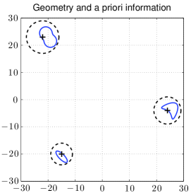
Example 9.1.

We consider a scattering problem with three obstacles as shown in figure 9.1 (left), which are illuminated by a plane wave $u^{i}(x)=e^{\mathrm{i}kx\cdot d}$, $x\in{\mathbb{R}}$, with incident direction $d=(1,0)$ and wave number $k=1$ (i.e., the wave length is $\lambda=2\pi\approx 6.28$).

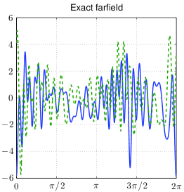
Figure 9.1: Left: Geometry of the scatterers (solid) and a priori information on the source locations (dashed). Right: Real part (solid) and imaginary part (dashed) of the far field $\alpha$.

Assuming that the ellipse is sound soft whereas the kite and the nut are sound hard, the scattered field $u^{s}$ satisfies the homogeneous Helmholtz equation outside the obstacles, the Sommerfeld radiation condition at infinity, and Dirichlet (ellipse) or Neumann boundary conditions (kite and nut) on the boundaries of the obstacles. We simulate the corresponding far field $\alpha$ of $u^{s}$ on an equidistant grid with $512$ points on the unit sphere $S^{1}$ using a Nyström method (cf. [3, 15]). Figure 9.1 (middle) shows the real part (solid line) and the imaginary part (dashed line) of $\alpha$. Since the far field $\alpha$ can be written as a superposition of three far fields radiated by three individual smooth sources supported in arbitrarily small neighborhoods of the scattering obstacles (cf., e.g., [19, lemma 3.6]), this example fits into the framework of the previous sections.

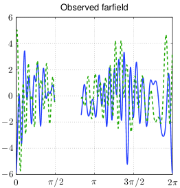
We assume that the far field cannot be measured on the segment

$$\Omega\,=\,\{\theta=(\cos t,\sin t)\in S^{1}\;|\;\pi/2<t<\pi/2+\pi/3\}\,,$$

i.e., $|\Omega|=\pi/3$. We first apply the least squares procedure and use the dashed circles shown in figure 9.1 (left) as a priori information on the approximate source locations $B_{R_{i}}(c_{i})$, $i=1,2,3$. More precisely, $c_{1}=(24,-4)$, $c_{2}=(-22,23)$, $c_{3}=(-15,-20)$ and $R_{1}=5$, $R_{2}=6$ and $R_{3}=4$. Accordingly we choose $N_{1}=7$, $N_{2}=9$ and $N_{3}=6$, and solve the linear system (9.2).

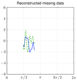
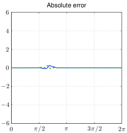
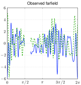
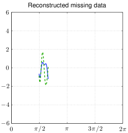
Figure 9.2: Reconstruction of the least squares scheme: Observed far field $\gamma$ (left), reconstruction of the missing part $\alpha|_{\Omega}$ (middle), and difference between exact far field and reconstructed far field (right).

Figure 9.2 shows a plot of the observed data $\gamma$ (left), of the reconstruction of the missing data segment obtained by the least squares algorithm and of the difference between the exact far field and the reconstructed far field. Again the solid line corresponds to the real part while the dashed line corresponds to the imaginary part. The condition number of the matrix is $5.4\times 10^{4}$. We note that the missing data component in this example is actually too large for the assumptions of theorem 5.7 to be satisfied. Nevertheless the least squares approach still gives good results.

Applying the (fast) iterative soft shrinkage algorithm to this example (with regularization parameter $\mu=10^{-3}$ in (9.4)) does not give a useful reconstruction. As indicated by the estimates in theorem 6.8 the ${l^{1}}$ approach seems to be a bit less stable. Hence we halve the missing data segment, consider in the following

$$\Omega\,=\,\{\theta=(\cos t,\sin t)\in S^{1}\;|\;\pi/2<t<\pi/2+\pi/6\}\,,$$

i.e., $|\Omega|=\pi/6$, and apply the ${l^{1}}$ reconstruction scheme to this data.

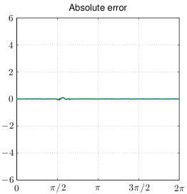
Figure 9.3: Reconstruction of the basis pursuit scheme: Observed far field $\gamma$ (left), reconstruction of the missing part $\alpha|_{\Omega}$ (middle), and difference between exact far field and reconstructed far field (right).

Figure 9.3 shows a plot of the observed data $\gamma$ (left), of the reconstruction of the missing data segment obtained by the fast iterative soft shrinkage algorithm (with $\mu=10^{-3}$) after $10^{3}$ iterations (the initial guess is zero) and of the difference between the exact far field and the reconstructed far field.

The behavior of both algorithms in the presence of noise in the data depends crucially on the geometrical setup of the problem (i.e. on its conditioning). The smaller the missing data segment is and the smaller the dimensions of the individual source components are relative to their distances, the more noise these algorithms can handle. $\lozenge$

Conclusions

We have considered the source problem for the two-dimensional Helmholtz equation when the source is a superposition of finitely many well-separated compactly supported source components. We have presented stability estimates for numerical algorithms to split the far field radiated by this source into the far fields corresponding to the individual source components and to restore missing data segments. Analytic and numerical examples confirm the sharpness of these estimates and illustrate the potential and limitations of the numerical schemes.

The most significant observations are:

• The conditioning of far field splitting and data completion depends on the dimensions of the source components, their relative distances with respect to wavelength and the size of the missing data segment. The results clearly suggest combining data completion with splitting whenever possible in order to improve the conditioning of the data completion problem.

• The conditioning of far field splitting and data completion depends on wave length and deteriorates with increasing wave number. Therefore, in order to increase resolution one not only has to increase the wave number but also the dynamic range of the sensors used to measure the far field data.

Appendix

Appendix A Some properties of the squared singular values $\{s_{n}^{2}(R)\}$ of $\mathcal{F}_{B_{R}(0)}$

In the following we collect some interesting properties of the squared singular values $\{s_{n}^{2}(R)\}$, as introduced in (3.3), of the restricted Fourier transform $\mathcal{F}_{B_{R}(0)}$ from (3.1).

We first note that [21, 10.22.5] implies that the squared singular values from (3.3) satisfy

$$s_{n}^{2}(R)\,=\,\pi R^{2}\bigl{(}J_{n}^{2}(R)-J_{n-1}(R)J_{n+1}(R)\bigr{)}\,,\qquad n\in{\mathbb{Z}}\,,$$

and simple manipulations using recurrence relations for Bessel functions

$$\frac{nJ_{n}(r)}{r} \,=\,\frac{J_{n+1}(r)+J_{n-1}(r)}{2}\,, n\in{\mathbb{Z}}\,,$$ (A.1a)

$$J_{n}^{\prime}(r) \,=\,\frac{J_{n-1}-J_{n+1}(r)}{2}\,, n\in{\mathbb{Z}}\,,$$ (A.1b)

(cf., e.g., [21, 10.6(i)]) show that, for $n\in{\mathbb{Z}}$

$$\begin{split}s_{n}^{2}(R)&\,=\,\pi\bigl{(}n^{2}J_{n}^{2}(R)-R^{2}J_{n-1}(R)J_{n+1}(R)+R^{2}J_{n}(R)-n^{2}J_{n}^{2}(R)\bigr{)}\\ &\,=\,\pi\Bigl{(}\frac{R^{2}}{4}(J_{n-1}(R)+J_{n+1}(R))^{2}-R^{2}J_{n-1}(R)J_{n+1}(R)+(R^{2}-n^{2})J_{n}^{2}(R)\Bigr{)}\\ &\,=\,\pi\Bigl{(}R^{2}\Bigl{(}\frac{J_{n-1}(R)-J_{n+1}(R)}{2}\Bigr{)}^{2}+(R^{2}-n^{2})J_{n}^{2}(R)\Bigr{)}\\ &\,=\,\pi\bigl{(}(RJ_{n}^{\prime}(R))^{2}+(R^{2}-n^{2})J_{n}^{2}(R)\bigr{)}\,.\end{split}$$ (A.2)

Lemma A.1.

$$\sum_{n=-\infty}^{\infty}s_{n}^{2}(R)\,=\,\pi R^{2}\,.$$

Proof.

Since

$$\sum_{n=-\infty}^{\infty}J_{n}^{2}(r)\,=\,1$$

(cf. [21, 10.23.3]), the definition (3.3) yields

$$\sum_{n=-\infty}^{\infty}s_{n}^{2}(R)\,=\,2\pi\int_{0}^{R}\Bigl{(}\sum_{n=-\infty}^{\infty}J_{n}^{2}(r)\Bigr{)}r\,\operatorname{d\!}r\,=\,2\pi\int_{0}^{R}r\,\operatorname{d\!}r\,=\,\pi R^{2}\,.$$

∎

The next lemma shows that odd and even squared singular values, $s_{n}^{2}(R)$, are monotonically decreasing for $n\geq 0$ and monotonically increasing for $n\leq 0$.

Lemma A.2.

$$s_{n-1}^{2}(R)-s_{n+1}^{2}(R)\,\geq\,0\,,\qquad n\geq 0\,.$$

Proof.

Using the recurrence relations (A.1) we find that

$$J_{n-1}^{2}(r)-J_{n+1}^{2}(r)\,=\,\frac{4n}{r}J_{n}(r)J_{n}^{\prime}(r)\,=\,\frac{2n}{r}(J_{n}^{2})^{\prime}(r)\,.$$

Thus,

$$\begin{split}s_{n-1}^{2}(R)-s_{n+1}^{2}(R)&\,=\,2\pi\Bigl{(}\int_{0}^{R}J_{n-1}^{2}(r)r\,\operatorname{d\!}r-\int_{0}^{R}J_{n+1}^{2}(r)r\,\operatorname{d\!}r\Bigr{)}\\ &\,=\,2\pi\int_{0}^{R}2n(J_{n}^{2})^{\prime}(r)\,\operatorname{d\!}r\,=\,4\pi nJ_{n}^{2}(R)\,\geq\,0\,.\end{split}$$

∎

Integrating sharp estimates for $J_{n}(r)$ from [17], we obtain upper bounds for $s_{n}^{2}(R)$ when $|n|\geq R>0$. Since $s_{n}^{2}(R)=s_{-n}^{2}(R)$, $n\in{\mathbb{Z}}$, it is sufficient to consider $n\geq R$.

Lemma A.3.

Suppose that $n\geq R>0$. Then

$$s_{n}^{2}(R)\,\leq\,\frac{\pi 2^{\frac{2}{3}}n^{\frac{2}{3}}}{3^{\frac{4}{3}}\bigl{(}\Gamma(\frac{2}{3})\bigr{)}^{2}}\Bigl{(}\frac{n+\frac{1}{2}}{n}\Bigr{)}^{n+1}\Bigl{(}\frac{R^{2}}{n^{2}}e^{1-\frac{R^{2}}{n^{2}}}\Bigr{)}^{n}\frac{R^{2}}{n^{2}}\,.$$

Proof.

From theorem 2 of [17] we obtain for $0<r\leq n$ that

$$J_{n}^{2}(r)\,\leq\,\frac{2^{\frac{2}{3}}}{3^{\frac{4}{3}}\bigl{(}\Gamma(\frac{2}{3})\bigr{)}^{2}}\frac{r^{2n}}{n^{2n+\frac{2}{3}}}e^{\frac{n^{2}-r^{2}}{n+\frac{1}{2}}}\,.$$

Substituting this into (3.3) yields

$$\begin{split}s_{n}^{2}(R)&\,\leq\,2\pi\frac{2^{\frac{2}{3}}}{3^{\frac{4}{3}}\bigl{(}\Gamma(\frac{2}{3})\bigr{)}^{2}}\frac{e^{\frac{n^{2}}{n+\frac{1}{2}}}}{n^{2n+\frac{2}{3}}}\int_{0}^{R}r^{2n}e^{-\frac{r^{2}}{n+\frac{1}{2}}}r\,\operatorname{d\!}r\\ &\,=\,\pi\frac{2^{\frac{2}{3}}}{3^{\frac{4}{3}}\bigl{(}\Gamma(\frac{2}{3})\bigr{)}^{2}}\frac{e^{\frac{n^{2}}{n+\frac{1}{2}}}}{n^{2n+\frac{2}{3}}}\Bigl{(}n+\frac{1}{2}\Bigr{)}^{n+1}\int_{0}^{\frac{R^{2}}{n+\frac{1}{2}}}t^{n}e^{-t}\,\operatorname{d\!}t\\ &\,\leq\,\pi\frac{2^{\frac{2}{3}}}{3^{\frac{4}{3}}\bigl{(}\Gamma(\frac{2}{3})\bigr{)}^{2}}\frac{e^{n}}{n^{2n+\frac{2}{3}}}\Bigl{(}n+\frac{1}{2}\Bigr{)}^{n+1}\int_{0}^{\frac{R^{2}}{n}}t^{n}e^{-t}\,\operatorname{d\!}t\,.\end{split}$$

Since $t^{n}e^{-t}$ is monotonically increasing for $0<t<\frac{R^{2}}{n}\leq n$, we see

$$\begin{split}s_{n}^{2}(R)&\,=\,\pi\frac{2^{\frac{2}{3}}}{3^{\frac{4}{3}}\bigl{(}\Gamma(\frac{2}{3})\bigr{)}^{2}}\frac{(n+\frac{1}{2})^{n+1}}{n^{2n+\frac{2}{3}}}e^{n}\frac{R^{2}}{n}\frac{R^{2n}}{n^{n}}e^{-\frac{R^{2}}{n}}\\ &\,=\,\pi\frac{2^{\frac{2}{3}}}{3^{\frac{4}{3}}\bigl{(}\Gamma(\frac{2}{3})\bigr{)}^{2}}n^{\frac{2}{3}}\Bigl{(}\frac{n+\frac{1}{2}}{n}\Bigr{)}^{n+1}\Bigl{(}\frac{R^{2}}{n^{2}}e^{1-\frac{R^{2}}{n^{2}}}\Bigr{)}^{n}\frac{R^{2}}{n^{2}}\,.\end{split}$$

∎

On the other hand, the squared singular values $s_{n}^{2}(R)$ are not small for $|n|<R$.

Theorem A.4.

Suppose that $R>n\geq 0$, define $\alpha\in(0,\frac{\pi}{2})$ by $\cos\alpha=\frac{n}{R}$, and therefore $\sin\alpha=\sqrt{1-(\frac{n}{R})^{2}}$, and assume $\alpha>\varepsilon>0$. Then

$$\biggl{|}J_{n}(R)-\sqrt{\frac{2}{\pi R\sin\alpha}}\cos\Bigl{(}R(\sin\alpha-\alpha\cos\alpha)-\frac{\pi}{4}\Bigr{)}\biggr{|} \,\leq\,\frac{C(\varepsilon)}{R}\,,$$ (A.3)

$$\biggl{|}J_{n}^{\prime}(R)+\sqrt{\frac{2}{\pi R\sin\alpha}}\sin\alpha\sin\Bigl{(}R(\sin\alpha-\alpha\cos\alpha)-\frac{\pi}{4}\Bigr{)}\biggr{|} \,\leq\,\frac{C(\varepsilon)}{R}\,.$$ (A.4)

where the constant $C(\varepsilon)$ depends on the lower bound $\varepsilon$ but is otherwise independent of $n$ and $R$.

Proof.

By definition,

$$J_{n}(R)\,=\,\frac{1}{2\pi}\int_{-\pi}^{\pi}e^{\mathrm{i}(R\sin{t}-n{t})}\,\operatorname{d\!}t\,=\,\frac{1}{2\pi}\int_{-\pi}^{\pi}e^{\mathrm{i}R(\sin{t}-{t}\cos\alpha)}\,\operatorname{d\!}t\,=\,\frac{1}{2\pi}\int_{-\pi}^{\pi}e^{\mathrm{i}R\phi({t})}\,\operatorname{d\!}t$$ (A.5)

with

$$\phi({t})\,=\,\sin{t}-{t}\cos\alpha\,,\quad\phi^{\prime}({t})\,=\,\cos{t}-\cos\alpha\,,\quad\phi^{\prime\prime}({t})\,=\,-\sin{t}\,.$$

The phase function $\phi$ has stationary points at $\pm\alpha$, and $\phi^{\prime\prime}$ vanishes at $0$ and $\pi$. We will apply stationary phase in a neighborhood of each stationary point. The neighborhood must be small enough to guarantee that $|\phi^{\prime\prime}({t})|$ is bounded from below there. Integration by parts will be used to estimate integral in regions where $\phi^{\prime}$ is bounded below. The hypothesis that $\alpha>\varepsilon>0$ will guarantee that the union of these two regions covers the whole interval $(-\pi,\pi)$.

To separate the two regions, let $a_{\varepsilon}(\tau)=a\bigl{(}\frac{\tau}{\varepsilon}\bigr{)}$, $\tau\in{\mathbb{R}}$, be a $C^{\infty}$ cutoff function satisfying

$$a_{\varepsilon}(\tau)\,=\,\begin{cases}1&\text{if }|\tau|>2\varepsilon\\ 0&\text{if }|\tau|<\varepsilon\end{cases}\qquad\text{and}\qquad|a_{\varepsilon}^{(j)}(\tau)|\,\leq\,\frac{C_{j}}{\varepsilon^{j}}$$

with the $C_{j}>0$ independent of $\varepsilon>0$. Define $A_{\varepsilon}({t}):=a_{\varepsilon}(\phi^{\prime}({t}))$, ${t}\in(-\pi,\pi)$, then

$$A_{\varepsilon}({t})\,=\,\begin{cases}1&\text{if }|\phi^{\prime}({t})|>2\varepsilon\,,\\ 0&\text{if }|\phi^{\prime}({t})|<\varepsilon\,.\end{cases}$$ (A.6)

Theorem 7.7.1 of [13] tells us that for any integer $k\geq 0$

$$\biggl{|}\int_{-\pi}^{\pi}e^{\mathrm{i}R\phi({t})}A_{\varepsilon}({t})\,\operatorname{d\!}t\biggr{|}\,\leq\,\frac{C}{R^{k}}\sum_{j=0}^{k}\sup_{{t}\in\operatorname{supp}A_{\varepsilon}}\biggl{|}\frac{A_{\varepsilon}^{(j)}({t})}{(\phi^{\prime}({t}))^{2k-j}}\biggr{|}\,\leq\,\frac{C}{R^{k}\varepsilon^{2k}}\sum_{j=0}^{k}C_{j}$$ (A.7)

with $C$ only depending on an upper bound for the higher order derivatives of $\phi$. For the second inequality we have used (A.6) and the fact that all higher derivatives of $\phi$ are bounded by 1.

We will estimate the remainder of the integral using Theorem 7.7.5 of [13], which tells us that, if $t_{0}$ is the unique stationary point of $\phi$ in the support of a smooth function $B$, and $|\phi^{\prime\prime}({t})|>\delta>0$ on the support of $B$, then

$$\biggl{|}\int_{-\pi}^{\pi}e^{\mathrm{i}R\phi({t})}B({t})\,\operatorname{d\!}t-\sqrt{\frac{2\pi\mathrm{i}}{R\phi^{\prime\prime}(t_{0})}}e^{\mathrm{i}R\phi(t_{0})}B(t_{0})\biggr{|}\,\leq\,\frac{C}{R}\sum_{j=0}^{2}\sup_{{t}\in\operatorname{supp}B}|B^{(j)}({t})|$$ (A.8)

with $C>0$ depending only on the lower bound $\delta$ for $|\phi^{\prime\prime}({t})|$ and an upper bound for higher derivatives of $\phi$ on the support of $B$. We will set $B=1-A_{\varepsilon}({t})$, which is supported in two intervals, one containing $\alpha$ and the other containing $-\alpha$, so (A.8), becomes

$$\biggl{|}\int_{-\pi}^{\pi}e^{\mathrm{i}R\phi({t})}(1-A_{\varepsilon}({t}))\,\operatorname{d\!}t-\sqrt{\frac{2\pi}{R\sin\alpha}}2\cos\Bigr{(}R(\sin\alpha-\alpha\cos\alpha)-\frac{\pi}{4}\Bigr{)}\biggr{|}\,\leq\,\frac{C}{R}\mathop{\sum}\limits_{j=0}^{2}\frac{C_{j}}{\varepsilon^{j}}$$ (A.9)

as long as $\varepsilon$ is chosen so that $|\phi^{\prime\prime}({t})|=|\sin({t})|\geq\delta$ on the support of $1-A_{\varepsilon}({t})$.

The following lemma suggests a proper choice of $\varepsilon$. ∎

Lemma A.5.

Let ${t}$ and $\alpha$ belong to $\bigl{[}0,\frac{\pi}{2}\bigr{]}$ then

$$|\cos{t}-\cos\alpha|\,<\,\varepsilon$$

implies that

$$\sin{t}\,>\,\sin\alpha-\frac{2\varepsilon}{\sin\alpha}\,.$$

Proof.

Since

$$\sin^{2}{t}-\sin^{2}\alpha\,=\,\cos^{2}\alpha-\cos^{2}{t}$$

we deduce

$$\sin{t}-\sin\alpha\,=\,\frac{\cos\alpha+\cos{t}}{\sin{t}+\sin\alpha}(\cos\alpha-\cos{t})\,.$$

Consequently

$$|\sin{t}-\sin\alpha|\,\leq\,\frac{2}{\sin\alpha}\varepsilon\,.$$

∎

End of proof of theorem A.4.

We choose $\varepsilon=\frac{\sin^{2}\alpha}{4}$ and assume that $|\phi^{\prime}(t)|=|\cos t-\cos\alpha|<\varepsilon$, then lemma A.5 gives $\sin{t}>\frac{\sin\alpha}{2}$. We use this value of $\varepsilon$ in (A.6), i.e.

$$|\phi^{\prime}({t})|\,>\,2\varepsilon\quad\text{on }\operatorname{supp}A_{\varepsilon}\qquad\text{and}\qquad|\phi^{\prime}({t})|\,<\,\varepsilon\quad\text{on }\operatorname{supp}(1-A_{\varepsilon})\,.$$

Accordingly,

$$|\phi^{\prime\prime}({t})|\,=\,|\sin{t}|\,>\,\frac{\sin\alpha}{2}\,=\,\sqrt{\varepsilon}\,=:\,\delta\qquad\text{on }\operatorname{supp}(1-A_{\varepsilon})\,.$$

Now, adding (A.7) and (A.9) establishes (A.3).

The calculation for (A.4) is analogous with (A.5) replaced by

$$J_{n}^{\prime}(R)\,=\,\frac{1}{2\pi}\int_{-\pi}^{\pi}\mathrm{i}\sin({t})e^{\mathrm{i}(R\sin{t}-n{t})}\,\operatorname{d\!}t\,=\,\frac{1}{2\pi}\int_{-\pi}^{\pi}\mathrm{i}\sin({t})e^{\mathrm{i}R\phi({t})}\,\operatorname{d\!}t\,,$$

which has the same phase and hence the same stationary points. The only difference is that the term $B(t_{0})$ in (A.8) at $t_{0}=\pm\alpha$ will be $\pm\mathrm{i}\sin\alpha$ rather than 1. ∎

We now combine (A.3) and (A.4) with the equality (A.2) to obtain, for $\cos\alpha=\frac{n}{R}<1-\varepsilon$

$$\bigl{|}s_{n}^{2}(R)-2R\sin\alpha\bigr{|}\,=\,\bigl{|}s_{n}^{2}(R)-2\sqrt{R^{2}-n^{2}}\bigr{|}\,\leq\,C(\varepsilon)\sqrt{R}\,.$$

Since equation (A.5) is only a valid definition of the Bessel function $J_{n}(R)$ when $n$ is an integer, we denote in the following by $\lceil\nu R\rceil$ is smallest integer that is greater than or equal to $\nu R$, so that we can state a convergence result.

Corollary A.6.

$$\lim_{R\rightarrow\infty}\frac{s_{\lceil\nu R\rceil}^{2}(R)}{2R}\,=\,\begin{cases}\sqrt{1-\nu^{2}}&\nu\leq 1\\ 0&\nu\geq 1\end{cases}$$

Appendix B Proof of estimate (4.11)

Let $n\in{\mathbb{Z}}$ and $\mu:=(2n+1)(2n+3)$. Theorem 2 of [16] establishes that for $r>\frac{\sqrt{\mu+\mu^{\frac{3}{2}}}}{2}$,

$$J_{n}^{2}(r)\,\leq\,\frac{4(4r^{2}-(2n+1)(2n+5))}{\pi((4r^{2}-\mu)^{\frac{3}{2}}-\mu)}\,.$$ (B.1)

The following lemma shows that, under the assumptions of theorem 4.6, the estimate (B.1) implies (4.11).

Lemma B.1.

Let $M,N\geq 1$ and $r>2(M+N+1)$, then

$$\sup_{-(M+N)<n<(M+N)}J_{n}^{2}(r)\,\leq\,\frac{b}{r}\qquad\text{with $b\approx 0.7595$}\,.$$

Proof.

Since $J_{-n}^{2}(r)=J_{n}^{2}(r)$ we may assume w.l.o.g. that $n\geq 0$. Let $\eta:=\sqrt{(n+\frac{1}{2})(n+\frac{3}{2})}$. Then $\frac{\mu}{4}=\eta^{2}=n^{2}+2n+\frac{3}{4}$, i.e.

$$\frac{3}{4}\,\leq\,\eta^{2}\,\leq\,(n+1)^{2}$$ (B.2)

and therefore our assumption $r>2(M+N+1)$ implies for $0\leq n<M+N$ that

$$r\,>\,2(n+1)\,\geq\,2\eta\,.$$ (B.3)

Accordingly,

$$\frac{1}{2}\sqrt{\mu+\mu^{\frac{3}{2}}}\,=\,\frac{1}{2}\sqrt{4\eta^{2}+(4\eta^{2})^{\frac{3}{2}}}\,=\,\eta\sqrt{1+\frac{1}{(4\eta^{2})^{\frac{1}{3}}}}\,\leq\,\eta\sqrt{1+\frac{1}{(4\bigl{(}\frac{3}{4}\bigr{)}^{2})^{\frac{1}{3}}}}\,\leq\,\sqrt{2}\eta\,\leq\,\frac{r}{\sqrt{2}}\,\leq\,r\,.$$

This shows that the assumptions of theorem 2 of [16] are satisfied.

Next we consider (B.1) and further estimate its right hand side:

$$\begin{split}J_{n}^{2}(r)&\,\leq\,\frac{4(4r^{2}-(2n+1)(2n+5))}{\pi((4r^{2}-\mu)^{3/2}-\mu)}\,\leq\,\frac{4(4r^{2}-4\eta^{2})}{\pi(8(r^{2}-\eta^{2})^{\frac{3}{2}}-4\eta^{2})}\\ &\,=\,\frac{2}{\pi}\frac{1}{(r^{2}-\eta^{2})^{\frac{1}{2}}}\frac{1}{1-\frac{1}{2}\frac{\eta^{2}}{(r^{2}-\eta^{2})^{\frac{3}{2}}}}\,=\,\frac{2}{\pi}\frac{1}{r}\frac{1}{\bigl{(}1-\bigl{(}\frac{\eta}{r}\bigr{)}^{2}\bigr{)}^{\frac{1}{2}}}\frac{1}{1-\frac{1}{2}\frac{\eta^{2}}{(r^{2}-\eta^{2})^{\frac{3}{2}}}}\,.\end{split}$$

Since $r>2(M+N+1)\geq 6$, applying (B.2) and (B.3) yields

$$\frac{\eta^{2}}{(r^{2}-\eta^{2})^{\frac{3}{2}}}\,=\,\frac{1}{r}\frac{\bigl{(}\frac{\eta}{r}\bigr{)}^{2}}{\bigl{(}1-\bigl{(}\frac{\eta}{r}\bigr{)}^{2}\bigr{)}^{\frac{3}{2}}}\,\leq\,\frac{1}{r}\frac{\frac{1}{4}}{\bigl{(}\frac{3}{4}\bigr{)}^{\frac{3}{2}}}\,=\,\frac{1}{3\sqrt{27}}\,,$$

whence

$$J_{n}^{2}(r)\,\leq\,\frac{2}{\pi}\frac{1}{r}\Bigl{(}\frac{4}{3}\Bigr{)}^{\frac{1}{2}}\frac{1}{1-\frac{1}{2}\frac{1}{3\sqrt{27}}}\,=\,\frac{b}{r}\qquad\text{with }b\approx 0.7595\,.$$

∎

Appendix C Some elementary inequalities

Here we prove some elementary inequalities that we haven’t been able to find in the literature.

Lemma C.1.

Let $a_{1},\ldots,a_{I}\in{\mathbb{R}}$. Then

• $$\sum_{i=1}^{I}\sum_{j\not=i}a_{i}a_{j}\,\leq\,(I-1)\sum_{i=1}^{I}a_{i}^{2}\,,$$ (C.1)

• $$\Bigl{(}\sum_{i=1}^{I}a_{i}\Bigr{)}^{2}\,\leq\,I\sum_{i=1}^{I}a_{i}^{2}\,,$$ (C.2)

• $$\sum_{i=1}^{I}\sum_{j\not=i}a_{i}a_{j}\,\leq\,\frac{I-1}{I}\Bigl{(}\sum_{i=1}^{I}a_{i}\Bigr{)}^{2}\,.$$ (C.3)

Proof.

• $$0\,\leq\,\sum_{i=1}^{I}\sum_{j\not=i}(a_{j}-a_{i})^{2}\,=\,\sum_{i=1}^{I}\sum_{j\not=i}(a_{i}^{2}-2a_{i}a_{j}+a_{j}^{2})\,=\,2(I-1)\sum_{i=1}^{I}a_{i}^{2}-2\sum_{i=1}^{I}\sum_{j\not=i}a_{i}a_{j}\,.$$

• Using (C.1) we find that

  $$\Bigl{(}\sum_{i=1}^{I}a_{i}\Bigr{)}^{2}\,=\,\sum_{i=1}^{I}a_{i}^{2}+\sum_{i=1}^{I}\sum_{j\not=i}a_{i}a_{j}\,\leq\,I\sum_{i=1}^{I}a_{i}^{2}\,.$$

• Proceeding as in (b) but applying (C.1) the other way round yields

  $$\Bigl{(}\sum_{i=1}^{I}a_{i}\Bigr{)}^{2}\,=\,\sum_{i=1}^{I}a_{i}^{2}+\sum_{i=1}^{I}\sum_{j\not=i}a_{i}a_{j}\,\geq\,\frac{I}{I-1}\sum_{i=1}^{I}\sum_{j\not=i}a_{i}a_{j}\,.$$

∎