Is there a concordance value for ?
Abstract
Context. We test the theoretical predictions of several cosmological models against different observables to compare the indirect estimates of the current expansion rate of the Universe determined from model fitting with the direct measurements based on Cepheids data published recently.
Aims. We perform a statistical analysis of type Ia supernova (SN Ia), Hubble parameter, and baryon acoustic oscillation data. A joint analysis of these datasets allows us to better constrain cosmological parameters, but also to break the degeneracy that appears in the distance modulus definition between and the absolute B-band magnitude of SN Ia, .
Methods. From the theoretical side, we considered spatially flat and curvature-free CDM, CDM, and inhomogeneous Lemaître-Tolman-Bondi (LTB) models. To analyse SN Ia we took into account the distributions of SN Ia intrinsic parameters.
Results. For the CDM model we find that , km sMpc, while the corrected SN absolute magnitude has a normal distribution . The CDM model provides the same value for , while km sMpc and . When an inhomogeneous LTB model is considered, the combined fit provides km sMpc.
Conclusions. Both the Akaike information criterion and the Bayes factor analysis cannot clearly distinguish between CDM and CDM cosmologies, while they clearly disfavour the LTB model. For the CDM, our joint analysis of the SN Ia, the Hubble parameter, and the baryon acoustic oscillation datasets provides values that are consistent with cosmic microwave background (CMB)-only Planck measurements, but they differ by from the value based on Cepheids data.
Key Words.:
cosmology: cosmological parameters, distance scale, dark matter, dark energy1 Introduction
Since the early determination by Hubble (Hubble, 1929), the Hubble constant was for a long time believed to be between 50 and 100 km sMpc (Kirshner, 2003). Recent findings are obtained by means of space facilities, improved control of systematics, and the use of different calibration techniques, as in the Hubble Space Telescope Key Project, which estimated km sMpc (Freedman et al., 2001). Riess et al. (2016) provided the most recent direct estimate of the expansion rate of the Universe: km sMpc. Together with these extraordinary improvements in the direct determination of the distance ladder, there are by now different classes of observations that allow an indirect estimate of the Hubble constant. Among others, the observations of the cosmic microwave background (CMB) anisotropy by WMAP (Hinshaw et al., 2013) and Planck Collaboration (2015) satellites yielded values of km sMpc and km sMpc, respectively. In addition to the CMB anisotropy measurements, other observables have been crucial to constrain the cosmological parameters, such as type Ia supernovae (SN Ia). The high-z supernova search team led by Adam Riess together with Brian P. Schmidt (Riess et al., 1998) and the supernova cosmology project led by Saul Perlmutter (Perlmutter et al., 1999) reported the first evidence for an accelerated cosmic expansion. Since then, the number of observed SN Ia increased by about an order of magnitude. Different publicly available compilations have been used to constrain cosmological models: Union2 (Amanullah et al., 2010), Union2.1 (Suzuki et al., 2012), Constitution set (Hicken et al., 2009), and JLA (Betoule et al., 2014). The results confirm the need for a late accelerated expansion of the Universe, consistent with the findings of the WMAP and Planck missions. Unfortunately, the observations of SN Ia by themselves are not able to provide a value for the local expansion rate of the Universe, , since this parameter is degenerate with the SN absolute magnitude. However, there are other cosmological observables that are more directly sensitive to the value of the Hubble constant. On one hand, passively evolving red galaxies, which are dominated by the older stellar population, whose age can be accurately estimated from a spectroscopic analysis (also known as cosmic chronometers), can be used to provide the redshift dependence of the expansion rate, , as suggested by Jimenez & Loeb (2002). Fitting these observational Hubble data (OHD), Liu et al. (2015) found a value of km sMpc. On the other hand, the baryon acoustic oscillation (BAO) data have been used to constrain the cosmological parameters, providing results that agree with the most recent findings of the Planck Collaboration. In particular, a recent estimate of the Hubble constant provides km sMpc (Cheng & Huang, 2015).
It is clear that the indirect estimates of the Hubble constant lead to lower values of compared to the direct measurements. Even the earlier estimate of km sMpc by Riess et al. (2011) and the latest one (Riess et al., 2016) contradict the most recent result from Planck (TT, TE, EE + lowP) at the and level, respectively. The question now is whether this difference hides new physics beyond what is by now commonly called the concordance model. This point has been addressed by Efstathiou (2014), who reanalysed the Cepheid data used by Riess et al. (2011). He obtained a value km sMpc, reducing the difference to Planck to only and concluding that there is no evidence for new physics (see also Chen & Ratra (2011) and Marra et al. (2013)). We here extend this discussion to determine whether any difference is present when observables other than CMB are considered. To do so, we perform a separate and a joint analysis of SN Ia, OHD, and BAO data. The joint analysis promises to provide more stringent constraints on the cosmological models, and to break the degeneracy between the SN absolute magnitude and the Hubble constant, which is peculiar to the SN analysis.
Several SN datasets (such as Union and Constitution) provide cosmological distance moduli that are derived assuming a flat CDM model. Hence, these datasets need to be treated with caution when used to constrain cosmological models that are different from CDM. We used the JLA dataset, which provides model-independent apparent magnitudes instead of model-dependent distance moduli. Moreover, the increase in the amount of data and the improvement in systematics imply that a more complete statistical analysis is necessary. We therefore followed the approach proposed by Trøst Nielsen et al. (2015) for the SN data analysis. For the theoretical models we considered the standard flat CDM model and its extensions, which include the curvature-free CDM model and a dark energy model characterised by an equation of state (EoS) , with . In addition, we also considered a different class of models, based on the Lemaître-Tolman-Bondi (LTB) metric, which describes an isotropic but inhomogeneous Universe (Lemaître, 1933; Tolman, 1934; Bondi, 1947; Krasiński, 1997), to stress the dependence of the Hubble constant estimates on the assumed theoretical model.
The plan of the paper is as follows. In Section 2 we review the theoretical models we considered. In Section 3 we review the observables and datasets used in our analysis. In Section 4 we show the results of our comparison between theory and observations. Finally, in Section 6 we summarise our findings and conclusions.
2 Theoretical models
All the models considered here arise from the exact solutions of the Einstein field equations (EE) , where is the Einstein tensor, , and is the form of the energy-momentum tensor for a perfect fluid in the comoving frame. Here and (pressure and density of the fluid) are related by the equation of state (EoS) .
2.1 Friedmann-Lemaître-Robertson-Walker models
Friedmann-Lemaître-Robertson-Walker (FLRW) models describe a homogeneous and isotropic Universe. Under such conditions, EE can be solved exactly, which results in the metric (Friedmann, 1922, 1924; Robertson, 1935; Walker, 1937)
| (1) |
where is a scale factor in units of length and is a curvature parameter for the open, flat, and closed 3D space geometry, respectively. The Hubble expansion rate as a function of redshift is defined as
| (2) |
Using the Friedmann equation, it can be expressed as
| (3) |
where , while the adimensional Hubble parameter is given by
| (4) |
Here and is the age of the Universe, while the sum runs over all the components of the cosmological fluid, which are each characterised by its own EoS and density parameter, , and the present density of the -th component in units of the critical density . The functional dependence of the luminosity distance with the redshift is fixed by the cosmological model. In the FLRW model is calculated according to the equation
| (5) |
where the function depends on the curvature,
| (6) |
Eqs. 3 and 5 are used in Section 4 to fit theoretical models to observables such as the Hubble expansion rate and the SN Ia.
There is overwhelming evidence that about a quarter of the critical density in the Universe is in the form of a cold, weakly interacting dark matter (CDM) and that an extra component in the cosmological fluid is needed for closing the Universe. Although the physical nature of this dark energy (DE) component is poorly understood, it currently provides the only explanation for the accelerated expansion of the Universe in a FLRW cosmology (Riess et al., 1998; Perlmutter et al., 1999). The second Friedmann equation
| (7) |
shows that for the cosmic fluid to be in an accelerated expansion, at least one component must have . The density evolution is provided by the time component of the conservation equations :
| (8) |
While DM is more constrained and commonly considered cold and pressureless (), the DE models consider various EoS for DE fluid. For , the DE density is constant (cf. Eq. 8) and can be described in terms of a non-vanishing cosmological constant . This case recovers the flat concordance CDM model considered to be the simplest way of best-fitting current cosmological observations. We also consider a CDM model with , which we assume to be constant with respect to the cosmic expansion.
2.2 LTB models
To explain the accelerated expansion suggested by SN Ia observations, the homogeneous and isotropic FLRW model must resort to DE. However, the same effect can be explained in an alternative way, by relaxing the homogeneity requirement of the cosmological principle and presuming an isotropic Gpc-size underdensity in matter distribution (see e.g. Alnes et al. (2006)). Under pressureless conditions, the local isotropic, but inhomogeneous Universe is described by the LTB metric
| (9) |
where determines the spatial curvature of 3D space. We denote derivatives with respect to the comoving radial coordinate and to the time with prime and dot, respectively. As before, is the scale factor in units of length, and we can introduce the reduced scale factor as well: , with . Unlike the standard model, the LTB model is characterised by radial and transverse expansion rates:
| (10) | ||||
| (11) |
Obviously, at the centre of symmetry . Then, the local expansion rate at the present time, , is given by
| (12) |
As in the FLRW metric, is an adimensional coordinate and not a measure of a physical distance. Being a flag coordinate, we have the freedom of rescaling such that, for example, . As we are considering an isotropic, but inhomogeneous fluid, all its parameters such as pressure, density, and EoS parameter may in principle depend not only on time, but also on the radial coordinate. For LTB models we consider the cosmic fluid with two components: the pressureless inhomogeneous cold matter (with ) and the DE fluid (with trivial EoS parameter ). Such a DE fluid component is equivalent to having an inhomogeneous term that is constant in time and on every sphere of radius , but with a possible radial profile . Recalling the Birkhoff theorem, we can expect that each shell evolves independently of the others, as a FLRW model with the same values of the fluid parameters. Hence, solving EE leads to the analogue of the Friedmann equation
| (13) |
Here . As in the FLRW model, , and are rescaled densities in units of the critical density. We still have for each shell . Eq. 13 is a differential equation for [cf. Eq. 11]. In the most general case, it can be solved only numerically. Here we concentrate our analysis on two special cases for which Eq. 13 can be solved analytically, namely and . The solution of the former is
| (14) | ||||
| (15) | ||||
| (16) |
where and are dimensionless parameters related to the conformal time, while is the Big Bang time of a given shell. We chose a homogeneous age of the Universe (in particular, ), as it has been shown that a Big Bang time different from shell to shell introduces decaying modes (Zibin, 2008), which in turn implies large CMB spectral distortions (Zibin, 2011). In the second simple case of the flat Universe we find a solution
| (17) |
Obviously, as , the profile of the term is defined by the profile of matter density. This case recovers the CDM model for . We here consider LTB models with a specific matter density profile:
| (18) |
where are the density parameters at the centre and beyond this underdensity (also called void), while the parameter defines its size. Clearly, for we recover a FLRW model with . We fixed the value of to unity for consistency with the inflationary paradigm. This simple density profile provides a smooth transition from the local to the distant matter density, without introducing too many free parameters. Furthermore, we assumed the observer to be located at the centre of the void. This is obviously a privileged position, against the Copernican principle, but the assumption can be relaxed with some complication of the mathematical formalism (Alnes & Amarzguioui, 2006). We will address these aspects in a forthcoming paper.
The two physical observables of interest, radial cosmic expansion rate and luminosity distance, are derived from observing photons that arrive radially in the chosen reference frame. Therefore, we used the relation of the two independent coordinates and with the redshift along the radial null geodesic (Enqvist & Mattsson, 2007)
| (19) | ||||
| (20) |
Finally, the solutions of Eqs. 19 and 20 can be used in combination with Eqs. 10 and 11 to relate any observable as a function of the redshift. The luminosity and the angular diameter distances in LTB model (see Ellis (2007)) are given by
| (21) |
and can be calculated numerically as functions of the redshift using the equations above.
3 Data analysis: methods
We tested the theoretical models described in Section 2 against a number of independent observables that are SN Ia, OHD, and BAO. Our goal is to address specifically the determination out of these measurements, also discussing the estimates of the other cosmological parameters. We analysed each of the datasets separately and then jointly to improve the sensitivity of our estimates.
3.1 SN Ia
The first dataset we consider is the JLA sample of SN Ia, for the reason we gave in the introduction. After a SN Ia is identified, the raw measurements are corrected for the Galactic extinction and the cross-filter change from observed band to the SN rest-frame B band. The JLA catalogue is built by processing these data with the use of the SALT light curve and spectral fitters (Guy et al., 2007), which provide the data points that can further be used in a cosmological study. Each SN is characterised by its redshift , the value for the maximum B-band apparent magnitude , then stretch and colour correction factors, and , respectively. Although considered the best-known high-redshift standard candles in cosmology, SN Ia still show small variations in their maximum absolute luminosity, and hence, in the B-band absolute magnitude, . To take this into account, the maximum absolute magnitude has been so far corrected through the empirical relation
| (22) |
where and the two correction parameters, and , are assumed to be constant for all the SN Ia (Hamuy et al., 1995; Kasen & Woosley, 2007). The distance modulus is related to the luminosity distance, , which contains all the cosmological information. Here, Mpc is the Hubble radius, while is a “Hubble constant-free” dimensionless luminosity distance, which depends on the other cosmological parameters. Therefore, the relation can be written as follows
| (23) |
This equation has so far been used to simultaneously fit the three nuisance parameters (, and ) together with the cosmological parameters relevant for the calculation of . It is evident that the distance moduli provided in SN datasets, depending on such estimates of the nuisance parameters, are consequently biased as a result of the pre-assumption of the CDM model. It follows from the definition of that the estimates of the cosmological parameters are insensitive to the actual value of , which plays the role of an overall offset in Eq. 23.
Assuming , and as constant means that every SN has the same corrected absolute magnitude and that no further corrections are needed. This statement has been questioned by Trøst Nielsen et al. (2015), who extended the procedure to consider the variation of the corrected absolute magnitude from one to another SN. For the sake of simplicity, , and are assumed to be independent Gaussian variables with normal distributions , and , respectively. In contrast, and are still considered constant coefficients of Eq. 22. Here we follow the same approach. Therefore, the joint probability for the values of the intrinsic SN parameters can be written as
| (24) |
where is a -vector of the true values of the intrinsic parameters for each of the supernovae; is a -vector with the central values of the parameter distributions; is the covariance matrix. The measured values (, , ) are conveniently expressed with the -vector . Following Trøst Nielsen et al. (2015), we define as the full set of free parameters, which describe both the astrophysical properties of SN and the cosmology. Then, the likelihood of the observed values, given the theoretical model , can conveniently be written as
| (25) |
where is the covariance matrix of the data (Betoule et al., 2014), and is the block-diagonal matrix
| (26) |
In analysing the JLA dataset by itself, we did not assume any prior on because we estimated the total offset . The distribution implies the distribution of : , with and . Hence, using this method, eight parameters describe the physics of SN Ia: , , , , , , , and (instead of three parameters, as in the conventional approach), which need to be fitted simultaneously with the cosmological parameters.
3.2 OHD
We have shown in Section 2. that the radial cosmic expansion rate is proportional to for FLRW (cf. Eq. 2) and LTB models (cf. Eqs. 10 and 20). Therefore, by measuring the age difference of two objects at two close redshift points, we can estimate the radial expansion rate at the corresponding redshift. For this purpose, Jimenez & Loeb (2002) proposed what is called the differential age (DA) method, which uses pairs of passively evolving red galaxies found at very similar redshifts. Another way to determine the expansion history of the Universe is using BAO (Gaztañaga et al., 2009; Delubac et al., 2015; Sahni et al., 2014). We here used the 23 DA points from the dataset collected and updated by Ding et al. (2015). The shape of the curve constrains the cosmological models, while the offset value provides the local cosmic expansion rate, . For this dataset, we performed a simple likelihood analysis considering that all the data points are uncorrelated,
| (27) |
Here is the observed value at redshift with its own uncertainty . For the theoretical prediction we used for either Eq. 3 for the FLRW models or Eq. 10 for LTB cosmologies.
3.3 BAO
The large-scale structure of the Universe has been extensively studied through redshift surveys, such as the six-degree field galaxy survey 6dFGS (Beutler et al., 2011) and the Sloan Digital Sky Survey-SDSS (Gil-Marín et al., 2015). The estimated galaxy correlation function shows a peak at large scales that is interpreted as the signature of the baryon acoustic oscillation in the relativistic plasma of the early Universe. In FLRW cosmology, the acoustic-scale distance ratio is defined by , where
| (28) |
is the comoving sound horizon at the redshift of the baryon drag epoch (Eisenstein et al., 1998), and
| (29) |
is a spherically averaged distance measure introduced by Eisenstein et al. (2005). In LTB cosmology, structure formation is poorly understood, which is the reason why using the BAO data for this model is still controversial (Zibin, 2008; Clarkson et al., 2009).
We used the measurements from the 6dFGS (Beutler et al., 2011), the SDSS DR7 (Ross et al., 2015), and the BOSS DR11 (Anderson et al., 2014) samples and the Ly forest measurements from BOSS DR11 (Delubac et al., 2015; Font-Ribera et al., 2014). The 6dFGS sample we used contains 75,117 galaxies up to and gives at an effective redshift . The SDSS DR7 catalogue contains 63,163 galaxies at and the measurement given is Mpc, where Mpc in their fiducial cosmology. BOSS DR11 contains nearly one million galaxies in the redshift range and the two measurements given are Mpc and Mpc with Mpc. The Ly forest of BOSS DR11 consists of 137,562 quasars in the redshift range and provides , at , and , at , where . To homogenise the measured BAO quantity as , we inverted the results of SDSS DR7 and BOSS DR11 using their fiducial values and combined the measurements of Ly forest from BOSS DR11 by means of Eq. 29. The observed values are shown in Table 1.
| Ref. | |||
| 0.106 | 0.336 | 0.015 | Beutler et al. (2011) |
| 0.15 | 0.2239 | 0.0084 | Ross et al. (2015) |
| 0.32 | 0.1181 | 0.0023 | Anderson et al. (2014) |
| 0.57 | 0.0726 | 0.0007 | Anderson et al. (2014) |
| 2.34 | 0.0320 | 0.0016 | Delubac et al. (2015) |
| 2.36 | 0.0329 | 0.0012 | Font-Ribera et al. (2014) |
The acoustic scale has also been measured by Kazin et al. (2014) using the WiggleZ galaxy survey. They reported three correlated measurements at redshifts 0.44, 0.60, and 0.73. However, we decided not to use these measurements because the WiggleZ volume partially overlaps that of the BOSS sample and the correlations between the two surveys have not been quantified.
As all the BAO data points in Table 1 are uncorrelated, we performed a simple likelihood analysis:
| (30) |
Here is the observed value at redshift with its own uncertainty (see Table 1). The theoretical estimate, , has been evaluated using Eqs. 29 and 28 and by exploiting the fitting formula for given in Eisenstein et al. (1998).
3.4 Combined analysis
We show in the next section that each of the three datasets we considered provides good estimates of the cosmological parameters. However, it is worthwhile combining all three datasets to obtain more stringent constraints. Moreover, the joint analysis allows us to provide separate estimates for the SN absolute magnitude and the Hubble constant. Assuming that the three datasets are independent, we evaluated the total likelihood as the product of the likelihoods of the single datasets. Therefore, for FLRW models , while for LTB cosmologies because in this case we did not consider the BAO dataset.
4 Data analysis: results
We present the results for cosmological models based on the FLRW and the LTB metrics. Several FLRW models have been analysed by Trøst Nielsen et al. (2015) using the JLA dataset, and we fully agree with their results. We extend their discussion to the CDM and LTB models, and also present the constraints derived from the OHD and BAO datasets. The JLA, OHD, and BAO data strongly constrain the apparent acceleration of the cosmic expansion, the current expansion rate, and the curvature of the Universe, respectively. A joint analysis, then, allows us to see what improvement we may have in the estimation of the cosmological parameters.
4.1 Constraints on flat CDM model
The flat CDM model has so far been tested with the available cosmological observables and is commonly considered the concordance model in cosmology.
| Data | [Mpc] | ||
| JLA | - | ||
| OHD | |||
| BAO | |||
| JLA+OHD | |||
| JLA+OHD+BAO |
The results of our analysis for this model are presented in Table 2. In particular, using the JLA dataset alone, we reproduce the value found by Trøst Nielsen et al. (2015). In addition to their results, we also quote the uncertainties in the parameter estimates, which show that the JLA dataset provides consistent results with those we find for OHD and BAO samples. However, our values for , obtained from JLA alone and JLA+OHD+BAO are both different by about 1.9 from the most recent determination of Planck (TT, TE, EE + lowP), which provided .
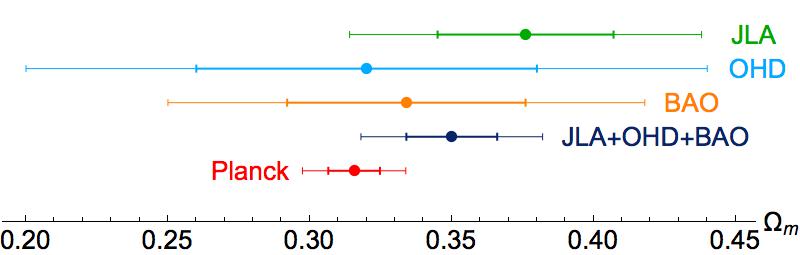
(a) Constraints on matter density
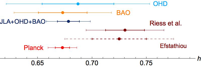 (b) Constraints on Hubble constant
The estimates derived from the OHD and BAO data for the current expansion rate are consistent by themselves and with Planck. The JLA dataset by itself is insensitive to . However, in the joint analysis JLA constrains other parameters of the fit, which in turn affect the estimate of . The final value for derived from the joint JLA+OHD+BAO analysis is in excellent agreement with the value from Planck (Figure 1), but is still different by and from the findings by Efstathiou (2014) and Riess et al. (2016).
4.2 Constraints on CDM model
This model is completely defined by the three cosmological parameters , , and . The best-fit values together with their statistical errors in Table 3 show a clear consistency of the results obtained by analysing the single datasets.
| Data | [Mpc] | ||
| JLA | - | ||
| OHD | |||
| BAO | |||
| JLA+OHD | |||
| JLA+OHD+BAO |
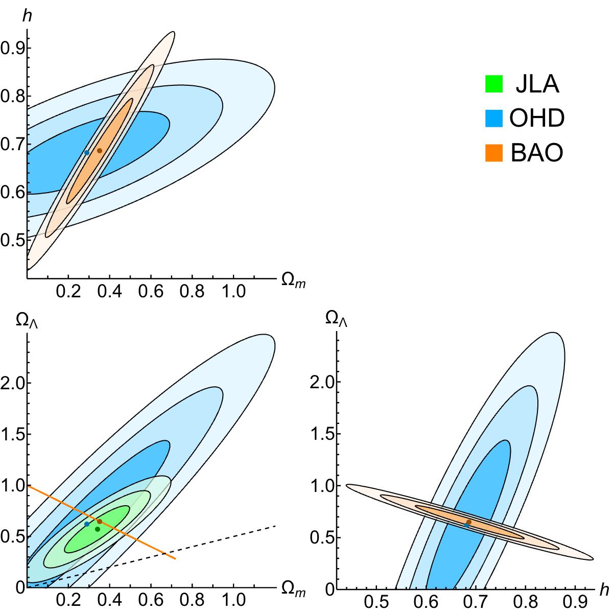
We present the confidence regions for the CDM model in Figure 2. Our results show that the BAO data constrain the curvature of the Universe quite strictly to be zero, leading to a strong correlation between and and shrinking the confidence regions to a line in plane. An alternative way to study the BAO data is by parametrising the CDM model with and . In this case, the result for is the same as in Table 3, while the best-fit value of is vanishingly small and consistent with zero. For this reason, the best-fit values of and are not exactly the same as those obtained for CDM (cf. Table 2), although they agree very well. The constraints from the JLA and OHD samples are fully consistent with the flat cosmology, although the best-fit values slightly differ from this line. The confidence regions in the and planes, resulting from the OHD and BAO data, fully overlap. The estimates for derived from the BAO and OHD analysis are consistent by themselves (see Table 3). In our full joint analysis, the CDM and the CDM models provide almost the same parameter estimates.
4.3 Constraints on CDM model
The CDM model considers a DE fluid with a free EoS parameter instead of a constant term corresponding to . The addition of one more parameter implies larger error bars in the and determinations presented in Table 4.
| Data | [Mpc] | ||
| JLA | - | ||
| OHD | |||
| BAO | |||
| JLA+OHD | |||
| JLA+OHD+BAO |
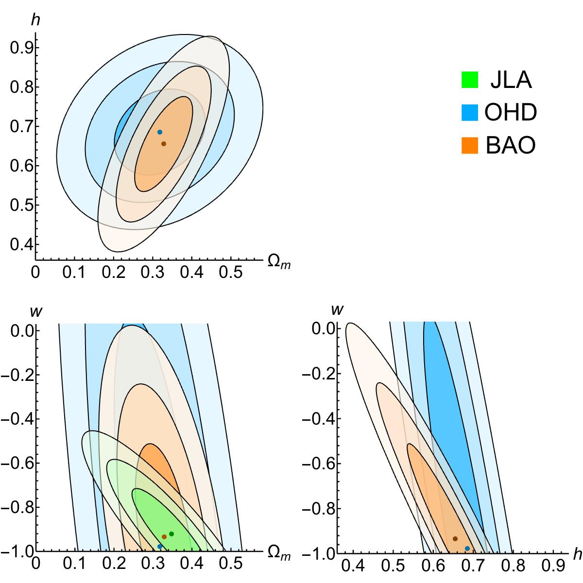
The confidence regions derived from the single datasets are consistent among themselves (see Figure 3). In particular, the estimates of are consistent with , the CDM model. The value of resulting from the full joint analysis is very close to the value obtained for the CDM model. The OHD and BAO estimates of are poorly constrained. However, again, the joint JLA+OHD+BAO analysis provides a value of that is different by and from the results of Efstathiou (2014) and Riess et al. (2016) , respectively.
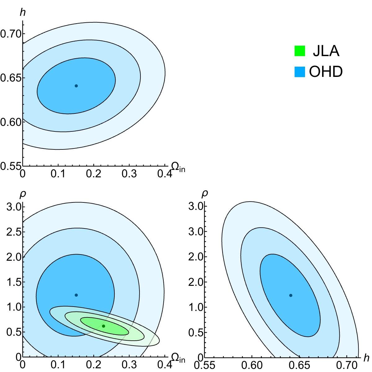
4.4 Constraints on LTB model
Here we extend the discussion of Trøst Nielsen et al. (2015) to consider LTB models. In the LTB model, the apparent acceleration of the local Universe arises because the matter density decreases radially from high to local redshifts. The radial matter density profile is in our case completely defined by Eq. 18, where we fixed and the remaining free parameters are the local value of the matter density and the dimensionless parameter , related to the size of the void. For the JLA data, these two are the only cosmological parameters in the fit because is included in the offset . Instead, for the OHD data we can fit all the three cosmological parameters.
| Data | [Mpc] | ||
| JLA | - | ||
| OHD | |||
| JLA+OHD |
The JLA sample constrains to be about a quarter of the critical density, while the value resulting from the OHD dataset is lower, but agrees within the errors (cf. Table 5). To gauge the physical size of the void, we considered the comoving angular diameter distance . The age of the Universe, , in the LTB model is related to through Eq. 14. Hence, we evaluated the angular diameter distance using km s. For the best-fit value from the JLA analysis we obtain Gpc. The OHD analysis prefers a much larger void, but with a profile consistent with the JLA data (see Figure 4).
We similarly performed a joint JLA+OHD analysis for the LTB model. The best-fit value is lower than the value obtained for CDM. This characteristic of LTB models has been observed in earlier works: our estimate is consistent within with the findings of Nadathur & Sarkar (2011) and at the level with the value from Freedman et al. (2001). However, our value differs by from the result of Efstathiou (2014) and by from the value given by Riess et al. (2016). These disagreements are even stronger than for the CDM model. In our analysis we also considered the LTB model, and found that it converges to CDM when both JLA and OHD datasets are used (see Table 6). The best-fit value of is equal to obtained for CDM, while the size of the void tends to infinity.
| Data | [Mpc] | ||
| JLA | - | ||
| OHD | |||
| JLA+OHD |
To better compare the considered cosmologies, we used the Akaike information criterion (AIC) and Bayes factor (). The Akaike estimate of minimum information (Akaike, 1974) for a given theoretical model and a given dataset is defined as
| (31) |
where is the number of independent parameters. By definition, this test gives preference to the model with the lowest AIC. In Table 7 we present the differences, (AIC), of the AIC values between each theoretical scenario and CDM. The Bayes factor similarly provides a criterion for choosing between two models by comparing their best likelihood values. The Bayes factor, represents the odds for the model against the alternative model . It is commonly considered that odds lower than 1:10 indicate a strong evidence against (Jeffreys, 1983). In reversed reading, odds greater than indicate a strong evidence against . In Table 7 we also show the Bayes factor of every model considered in this work against CDM.
| Model | (AIC) | |
| CDM | 0 | 1 |
| CDM | 1.69 | |
| CDM | 1.40 | |
| LTB | 9.41 | |
| LTB | 2 |
The standard CDM model is preferred by the Akaike criterion for fitting the JLA+OHD data. We note that the CDM and CDM models both have one parameter more than CDM. Nevertheless, the latter still has a lower AIC value, since the Akaike criterion rewards the model with fewer parameters. The LTB model is strongly disfavoured over CDM by both the AIC criterion and the Bayes factor. This behaviour mostly arises from the SN data. From our fit to the OHD data alone we obtain values of and for LTB and CDM, from which we conclude that LTB can be used to fit OHD data, as found by Wang & Zhang (2012). However, after using the JLA dataset alone with the Trøst Nielsen et al. (2015) approach, we obtain values of and for the LTB and CDM models, respectively. We therefore conclude that the LTB model is not performing as well as the concordance model in fitting the SN Ia data. This is in contrast to the previous findings in the literature (Alnes et al., 2006; Garfinkle, 2006; Blomqvist & Mörtsell, 2010), and consistent with the work by Vargas et al. (2015).
4.5 SN Ia intrinsic parameters
When performing the combined analysis, we were able to simultaneously fit all the cosmological parameters and the eight intrinsic astrophysical parameters of SN Ia. The latter are those characterising the normal distributions , and , and the constant coefficients and of Eq. 22.
| 0.108 0.005 | 0.038 0.038 | 0.932 0.027 | |
| -0.016 0.005 | 0.071 0.002 | 0.134 0.006 | 3.059 0.087 |
As an example, we present in Table 8 estimates of these nuisance parameters for the CDM model as they result from a combined fit with all the three datasets. The peak luminosity of SN does not have a constant value even after the corrections for the stretch and colour factors: the variation in the corrected SN Ia absolute magnitude is about at the level. In addition to light-curve shape and colour, the peak luminosity was similarly correlated to other parameters, including the host galaxy mass and the metallicity (Kelly et al., 2010; Hayden et al., 2013). Even these effects can be naturally taken into account in the distribution , considering that any additional correlations are expected to decrease the distribution width. Interestingly enough, the best-fit results of the SN parameters seem to be independent of the cosmological model under consideration: changing the model at most introduces variations on the last significant digit in the numbers given in Table 8. The only exception is the central value of obtained from the combined JLA+OHD fit for the LTB model: . This is due to the lower value of resulting from the fit to the OHD data.
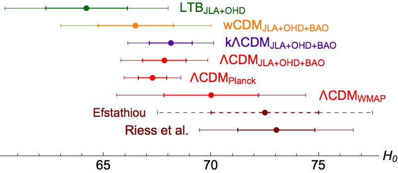
5 Indirect estimates
The estimates of the Hubble constant from our joint analysis and from WMAP and Planck are shown in Figure 5 together with the most recent direct estimates by Efstathiou (2014) and Riess et al. (2016). The excellent agreement between our value of for CDM and the CMB-only Planck measurement is remarkable, as is the consistency of the results we obtained for different FLRW cosmologies. On the other hand, the value of in LTB is lower than those of the FLRW models.
The indirect estimates of result to be systematically lower than the direct estimates. The best-fit values of for the CDM and the LTB models differ by and from the value of Efstathiou (2014), and differ by and from the result of Riess et al. (2016). For CDM, Riess et al. (2016) suggested that an additional source of dark radiation in the early Universe might allow a best-fit of the Planck data with a higher value for . This change would certainly affect the value of the sound horizon and consequently our estimate from BAO. However, this change cannot affect our result from the JLA+OHD analysis, which still differs by 2.4 from the results of Riess et al. (2016) and completely agrees with Planck. We conclude that this difference cannot be eliminated by changing in the concordance model or by invoking possible systematic uncertainties in the CMB measurements. If this were the case, we would not have found a good agreement between our JLA+OHD+BAO result and Planck (TT, TE, EE + lowP).
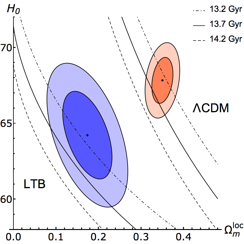
In a cosmological model, the age of the Universe, , is completely defined by the estimates. Here we used the result of our combined analysis for the Hubble constant to compare with the estimate of the absolute ages of stellar systems (Bono et al., 2010; Monelli et al., 2015). There is a quite good convergence on the value Gyr from different classes of observations (see, for a review, Freedman & Madore (2010)). Therefore, we show in Figure 6 the iso-ages corresponding to 13.2, 13.7, and 14.2 Gyr for the CDM and LTB models. We show the theoretical predictions in the same plane, where the local matter density corresponds to or to for the CDM or LTB model, respectively. Our estimates for the age of the Universe derived from the best-fit results of the combined analysis described above are Gyr for CDM and Gyr for LTB. In Figure 6 we also show the and confidence regions resulting from the JLA+OHD+BAO analysis for the CDM model, and those obtained from the JLA+OHD analysis for LTB. They are completely consistent with the observational estimate of quoted above.
6 Summary and conclusions
The combined analysis of JLA, OHD and BAO datasets allowed us to reach more stringent constraints on the cosmological parameters111Our analysis has been implemented in Mathematica 10. The code is available upon request. and to break the degeneracy between the SN absolute magnitude and the cosmic expansion rate. Our main findings can be summarised as follows.
By fitting the cosmological and the SN intrinsic parameters to the combined set of JLA, OHD, and BAO data, we constrained the distributions of SN absolute magnitude, stretch, and colour. The resulting values are cosmological-model independent, with the exception of the value obtained for LTB. The method we used can in principle be extended to include the effects related to mass and metallicity of the host galaxies.
We studied the CDM model and its extensions to consider non-vanishing spatial curvature and different assumptions for the DE component. The combined analysis clearly prefers the concordance model, as it forces the curvature to vanish and the DE EoS to be consistent with .
We also studied an LTB model with a Gaussian profile, which is strongly disfavoured with respect to the concordance model by information criteria, such as AIC analysis or Bayes factor.
For the CDM model, the JLA+OHD+BAO analysis provides a value of km sMpc that is fully consistent with the Planck (TT, TE, EE + lowP) result. This means that the difference with the direct measurements by Riess et al. (2016) is very likely not due to systematics in the Planck CMB measurements. It also seems difficult to reconcile direct and indirect measurements by considering an additional source of dark radiation in the early Universe, as this would not affect the JLA+OHD fit, which is still consistent with Planck. Therefore, it is still unclear wether it is necessary to extend the concordance CDM model.
Acknowledgements.
We are grateful to Jeppe Trøst Nielsen for useful discussions on the JLA data analysis, and to Martin White for his advice about the BAO data. We thank Giuseppe Bono and the referee for their constructive comments and helpful suggestions.References
- Akaike (1974) Akaike, H. 1974, IEEE Transactions on Automatic Control, 19, 716
- Alnes & Amarzguioui (2006) Alnes, H. & Amarzguioui, M. 2006, Phys. Rev. D, 74, 103520
- Alnes et al. (2006) Alnes, H., Amarzguioui, M., & Grøn, Ø. 2006, Phys. Rev. D, 73, 083519
- Amanullah et al. (2010) Amanullah, R., Lidman, C., Rubin, D., et al. 2010, ApJ, 716, 712
- Anderson et al. (2014) Anderson, L., Aubourg, É., Bailey, S., et al. 2014, MNRAS, 441, 24
- Betoule et al. (2014) Betoule, M., Kessler, R., Guy, J., et al. 2014, A&A, 568, A22
- Beutler et al. (2011) Beutler, F., Blake, C., Colless, M., et al. 2011, MNRAS, 416, 3017
- Blomqvist & Mörtsell (2010) Blomqvist, M. & Mörtsell, E. 2010, J. Cosmology Astropart. Phys., 5, 006
- Bondi (1947) Bondi, H. 1947, MNRAS, 107, 410
- Bono et al. (2010) Bono, G., Stetson, P. B., VandenBerg, D. A., et al. 2010, ApJ, 708, L74
- Chen & Ratra (2011) Chen, G. & Ratra, B. 2011, PASP, 123, 1127
- Cheng & Huang (2015) Cheng, C. & Huang, Q. 2015, Science China Physics, Mechanics, and Astronomy, 58, 095684
- Clarkson et al. (2009) Clarkson, C., Clifton, T., & February, S. 2009, J. Cosmology Astropart. Phys., 6, 25
- Delubac et al. (2015) Delubac, T., Bautista, J. E., Busca, N. G., et al. 2015, A&A, 574, A59
- Ding et al. (2015) Ding, X., Biesiada, M., Cao, S., Li, Z., & Zhu, Z.-H. 2015, ApJ, 803, L22
- Efstathiou (2014) Efstathiou, G. 2014, MNRAS, 440, 1138
- Eisenstein et al. (1998) Eisenstein, D. J., Hu, W., & Tegmark, M. 1998, ApJ, 504, L57
- Eisenstein et al. (2005) Eisenstein, D. J., Zehavi, I., Hogg, D. W., et al. 2005, ApJ, 633, 560
- Ellis (2007) Ellis, G. F. R. 2007, General Relativity and Gravitation, 39, 1047
- Enqvist & Mattsson (2007) Enqvist, K. & Mattsson, T. 2007, J. Cosmology Astropart. Phys., 2, 19
- Font-Ribera et al. (2014) Font-Ribera, A., Kirkby, D., Busca, N., et al. 2014, J. Cosmology Astropart. Phys., 5, 27
- Freedman & Madore (2010) Freedman, W. L. & Madore, B. F. 2010, ARA&A, 48, 673
- Freedman et al. (2001) Freedman, W. L., Madore, B. F., Gibson, B. K., et al. 2001, ApJ, 553, 47
- Friedmann (1922) Friedmann, A. 1922, Zeitschrift fur Physik, 10, 377
- Friedmann (1924) Friedmann, A. 1924, Zeitschrift fur Physik, 21, 326
- Garfinkle (2006) Garfinkle, D. 2006, Classical and Quantum Gravity, 23, 4811
- Gaztañaga et al. (2009) Gaztañaga, E., Cabré, A., & Hui, L. 2009, MNRAS, 399, 1663
- Gil-Marín et al. (2015) Gil-Marín, H., Percival, W. J., Cuesta, A. J., et al. 2015, arXiv:1509.06373
- Guy et al. (2007) Guy, J., Astier, P., Baumont, S., et al. 2007, A&A, 466, 11
- Hamuy et al. (1995) Hamuy, M., Phillips, M. M., Maza, J., et al. 1995, AJ, 109, 1
- Hayden et al. (2013) Hayden, B. T., Gupta, R. R., Garnavich, P. M., et al. 2013, ApJ, 764, 191
- Hicken et al. (2009) Hicken, M., Wood-Vasey, W. M., Blondin, S., et al. 2009, ApJ, 700, 1097
- Hinshaw et al. (2013) Hinshaw, G., Larson, D., Komatsu, E., et al. 2013, ApJS, 208, 19
- Hubble (1929) Hubble, E. 1929, Proceedings of the National Academy of Science, 15, 168
- Jeffreys (1983) Jeffreys, H. S. 1983, Theory of probability, The International series of monographs on physics (Oxford: Clarendon Press New York)
- Jimenez & Loeb (2002) Jimenez, R. & Loeb, A. 2002, ApJ, 573, 37
- Kasen & Woosley (2007) Kasen, D. & Woosley, S. E. 2007, ApJ, 656, 661
- Kazin et al. (2014) Kazin, E. A., Koda, J., Blake, C., et al. 2014, MNRAS, 441, 3524
- Kelly et al. (2010) Kelly, P. L., Hicken, M., Burke, D. L., Mandel, K. S., & Kirshner, R. P. 2010, ApJ, 715, 743
- Kirshner (2003) Kirshner, R. P. 2003, Proceedings of the National Academy of Science, 101, 8
- Krasiński (1997) Krasiński, A. 1997, Inhomogeneous Cosmological Models (Cambridge University Press), cambridge Books Online
- Lemaître (1933) Lemaître, G. 1933, Annales de la Société Scientifique de Bruxelles, 53, 51
- Liu et al. (2015) Liu, Z.-E., Qin, H.-F., Zhang, T.-J., Wang, B.-Q., & Bi, S.-L. 2015, arXiv:1501.04176
- Marra et al. (2013) Marra, V., Amendola, L., Sawicki, I., & Valkenburg, W. 2013, Phys. Rev. Lett., 110, 241305
- Monelli et al. (2015) Monelli, M., Testa, V., Bono, G., et al. 2015, ApJ, 812, 25
- Nadathur & Sarkar (2011) Nadathur, S. & Sarkar, S. 2011, Phys. Rev. D, 83, 063506
- Perlmutter et al. (1999) Perlmutter, S., Aldering, G., Goldhaber, G., et al. 1999, ApJ, 517, 565
- Planck Collaboration (2015) Planck Collaboration. 2015, arXiv:1502.01589
- Riess et al. (1998) Riess, A. G., Filippenko, A. V., Challis, P., et al. 1998, AJ, 116, 1009
- Riess et al. (2011) Riess, A. G., Macri, L., Casertano, S., et al. 2011, ApJ, 730, 119
- Riess et al. (2016) Riess, A. G., Macri, L. M., Hoffmann, S. L., et al. 2016, arXiv:1604.01424v1
- Robertson (1935) Robertson, H. P. 1935, ApJ, 82, 284
- Ross et al. (2015) Ross, A. J., Samushia, L., Howlett, C., et al. 2015, MNRAS, 449, 835
- Sahni et al. (2014) Sahni, V., Shafieloo, A., & Starobinsky, A. A. 2014, ApJ, 793, L40
- Suzuki et al. (2012) Suzuki, N., Rubin, D., Lidman, C., et al. 2012, ApJ, 746, 85
- Tolman (1934) Tolman, R. C. 1934, Proceedings of the National Academy of Science, 20, 169
- Trøst Nielsen et al. (2015) Trøst Nielsen, J., Guffanti, A., & Sarkar, S. 2015, arXiv:1506.01354
- Vargas et al. (2015) Vargas, C. Z., Falciano, F. T., & Reis, R. R. R. 2015, arXiv:1512.02571
- Walker (1937) Walker, A. G. 1937, Proceedings of the London Mathematical Society, s2-42, 90
- Wang & Zhang (2012) Wang, H. & Zhang, T.-J. 2012, ApJ, 748, 111
- Zibin (2008) Zibin, J. P. 2008, Phys. Rev. D, 78, 043504
- Zibin (2011) Zibin, J. P. 2011, Phys. Rev. D, 84, 123508