Magnetic anisotropy in the Kitaev model systems Na2IrO3 and RuCl3
Abstract
We study the ordered moment direction in the extended Kitaev-Heisenberg model relevant to honeycomb lattice magnets with strong spin-orbit coupling. We utilize numerical diagonalization and analyze the exact cluster groundstates using a particular set of spin coherent states, obtaining thereby quantum corrections to the magnetic anisotropy beyond conventional perturbative methods. It is found that the quantum fluctuations strongly modify the moment direction obtained at a classical level, and are thus crucial for a precise quantification of the interactions. The results show that the moment direction is a sensitive probe of the model parameters in real materials. Focusing on the experimentally relevant zigzag phases of the model, we analyze the currently available neutron and resonant x-ray diffraction data on Na2IrO3 and RuCl3, and discuss the parameter regimes plausible in these Kitaev-Heisenberg model systems.
pacs:
75.10.Jm, 75.25.Dk, 75.30.EtI Introduction
Due to their intermediate spatial extension, -electrons in transition metal compounds comprise both the localized and itinerant features. This duality is manifested in a rich variety of metal-insulator transitions [1; 2]. Even deep in the Mott-insulating phase, the -electrons partially retain their kinetic energy, by making virtual hoppings to the neighboring sites and forming the covalent bonds. The internal structure of these bonds is dictated by the orbital shape of -electrons as well as by Pauli principle and Hund’s interactions among spins. This results in an intimate link between the nature of chemical bonds (“orbital order”) and magnetism [3], which can be cast in terms of phenomenological Goodenough-Kanamori rules.
The Kugel-Khomskii models [4] form a theoretical framework where the “spin physics” and “orbital chemistry” are treated on equal footing. A special feature of these models is that the -orbital is spatially anisotropic and hence cannot satisfy all the bonds simultaneously. In high symmetry crystals, this results in a picture of fluctuating orbitals [5; 6], where the frustration among different covalent bonds is resolved by virtue of their quantum superposition, lifting the orbital degeneracy without a static order.
It might seem that a relativistic spin-orbit coupling, which lifts the orbital degeneracy already on a single ion level [3; 4], will readily eliminate the orbital frustration problem. This coupling does indeed greatly reduce the initially large spin-orbital Hilbert space of -ions, leaving often just a twofold degenerate Kramers level with an effective (“pseudo”) spin one-half [7]. It turns out, however, that the pseudospins still well “remember” the orbital frustration, by inheriting the bond-directional nature of orbital interactions via the spin-orbit entanglement [6].
The bond-directional nature of pseudospin interactions has profound consequences for magnetism (as well as for the properties of doped systems [8]). The most remarkable example, pointed out in Ref. 9, is a possible realization of the Kitaev’s honeycomb model [10] in materials with the electronic configuration such as Na2IrO3. This theoretical proposal has sparked a broad interest in honeycomb lattice pseudospin systems (see the recent review article [11] and references therein).
There is a direct experimental evidence [12] that the Kitaev-type interactions are indeed dominant in Na2IrO3. Unusual features pointing towards the Kitaev model has been observed [13] also in spin excitation spectra of RuCl3 (this compound was suggested [14] to host pseudospin physics, too). On the other hand, it is also clear that there are terms in the pseudospin Hamiltonian that take these systems away from the Kitaev spin-liquid phase window [15]. The identification of these “undesired” interactions and clarification of their dependence on material parameters is an important issue that has been in the focus of many recent studies.
Experimentally, the strength of a dominant Kitaev coupling can readily be evaluated from an overall bandwidth of spin excitations; however, the determination of its sign and quantification of the subdominant terms is not straightforward and needs a theory support. The aim of this paper is to show that the direction of the ordered moments, which can be extracted from the neutron and x-ray diffraction data, contains a valuable information on the model parameters, including the sign of . Considering a symmetry dictated form of the model Hamiltonian, we calculate the pseudospin direction fully including quantum fluctuations which are expected to be crucial in frustrated spin models. We will point out that the pseudospin itself is not directly probed by neutrons; rather, they detect the direction of the magnetic moment which is not the same as that of the pseudospin. Similarly, we will describe how to extract the pseudospin direction from resonant x-ray scattering (RXS) data.
The paper is organized as follows. Section II introduces the model Hamiltonian. Section III briefly discusses the pseudospin easy axis direction on a classical level. Section IV introduces the method of deriving the moment direction from exact diagonalization (ED) data. Section V presents the ED results on moment direction as a function of model parameters. Section VI considers a relation between the pseudospins and magnetic moments probed by neutron diffraction and RXS experiments, and discusses implications of the theory for Na2IrO3 and RuCl3. Appendix A compares the method of Sec. IV with the standard approach. Appendix B derives the equations used in the analysis of RXS data. Finally, Appendix C discusses how the trigonal field can be extracted from magnetic excitation spectra.
II Extended Kitaev-Heisenberg model
To describe the interactions among the pseudospins (referred to as “spins” below), we adopt a model containing all symmetry allowed nearest-neighbor (NN) terms and the longer-range Heisenberg interactions
| (1) |
The nearest neighbor contribution is the extended Kitaev-Heisenberg model [16; 17; 18] that, apart from the Heisenberg interaction, includes all the bond-anisotropic interactions compatible with the symmetries of a trigonally-distorted honeycomb lattice. Its -bond contribution (see Fig. 1 for the definitions of the bonds and spin axes) takes the following form:
| (2) |
The Hamiltonian contributions for the other bonds ( and ) are obtained by a cyclic permutation among . The resulting alternation of the local easy axis directions from bond-to-bond, imposed by the Ising-like term , brings about a strong frustration which, as discussed above, can be traced back to the orbital frustration problem in Kugel-Khomskii type models. An extensive discussion of the above Hamiltonian and its nontrivial symmetry properties can be found in Ref. 19.
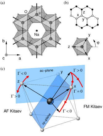
With the Kitaev-coupling alone, the model has a spin-liquid ground state. Both Na2IrO3 and RuCl3 show spin order where the zigzag-type ferromagnetic (FM) chains, running along -direction, are coupled to each other antiferromagnetically (AF), see Fig. 1(b). This order becomes a ground state of the Kitaev model with (AF sign), when a small FM Heisenberg coupling is added [20]. If the Kitaev coupling is negative, (FM sign), then zigzag order emerges due to longer-range AF couplings [21; 22] and/or terms [17; 18; 19]. Given that the stability of the Kitaev-liquid phase against perturbations strongly depends on the sign of [20], which scenario is realized in a given compound becomes an important issue.
Leaving aside the “orbital chemistry” aspects that decide the sign of as well as the other model parameters, we just mention that various ab-initio estimates (see, e.g., [16; 23; 24]) generally support FM regime, most likely reflecting the decisive role of Hund’s coupling effect on emphasized earlier [9; 15]. However, we take here a phenomenological approach, considering the model with free parameter values including both signs of . The , , and values are varied such that the ground state stays within the zigzag phase. Based on a recent result [24] that third-NN Heisenberg coupling is more significant than second-NN in both Na2IrO3 and RuCl3, we replace in (1) by , reducing thereby the parameter space.
The magnetic anisotropy in the present model is a nontrivial problem, since the leading term is anisotropic by itself, and, on top of this highly frustrated interaction, the other terms which eventually drive a magnetic order in real compounds have a strong impact on magnetic energy profile. As illustrated in Fig. 1(c) and discussed in detail below, the ordered moment direction is very sensitive to the model parameters, and it shows a qualitatively different behavior in case of FM and AF Kitaev couplings. We note that the “moment direction” in this figure refers to that of pseudospin; Section VI explains how it is related to the magnetic moments probed by neutron and x-ray diffraction experiments.
III Classical Moment direction
Let us briefly mention the results of a classical analysis (for details see Appendix B of Ref. 19) assuming the zigzag order with antiferromagnetic -bonds as shown in Fig. 1(b). On this level, the moment direction is determined solely by the anisotropy parameters , , and and corresponds to the eigenvector of the matrix
| (3) |
that has the lowest eigenvalue. This minimizes the anisotropic contribution in the classical energy per site of the zigzag phase, , where is a unit vector. The dominant Kitaev interaction contributing by the diagonal terms makes the main choice – it prefers either the -plane (FM ) or the -axis (AF ). The smaller and terms lead to a finer selection of the ordered moment direction.
In the case of the zigzag order stabilized by AF and FM , the ordered moment direction is close to the -axis being slightly tilted in the -plane mainly by virtue of [see Fig. 1(c)].
The FM case, where the zigzag order is stabilized by and terms, is more complex. With , the entire -plane is degenerate on a classical level. Further selection depends on the sign of , with the positive and negative sign making the moment to jump into the -plane or the -axis in the honeycomb plane, respectively. In the former case, an increasing further pushes the moment closer to the honeycomb plane. As it has been found earlier [15; 25] and discussed below, the Kitaev term generates an additional magnetic anisotropy due to quantum and/or thermal fluctuations, pinning the moment direction to the cubic axes. This will turn the above jumps into a gradual rotation of the easy axis with changing , along the path shown in Fig. 1(c).
IV Extraction of the moment direction from a cluster groundstate
To determine the groundstate of the Hamiltonian (1) and obtain the moment direction as a function of model parameters more rigorously than in the previous perturbative methods, we have performed an exact diagonalization using a hexagon-shaped 24-site supercell covering the honeycomb lattice. This cluster is highly symmetric and compatible with all the hidden symmetries of the model [19] so that no bias induced by the cluster geometry is expected.
Since the cluster groundstate does not spontaneously break the symmetry and corresponds to a superposition of all possible degenerate orderings, the identification of the ordered moment direction is not straightforward. One possibility is to evaluate the correlation matrix () at the ordering vector and to take the direction of the eigenvector corresponding to its largest eigenvalue. Because of specific problems of this standard approach in the present context (see Appendix A for details), we have developed here another method that brings a more intuitive picture of the exact groundstate by “measuring” the presence of the classical states with a varying moment direction. As a basic building block, we utilize the spin- coherent state
| (4) |
that is fully polarized along -direction [26]. Here the cubic axes are used as a convenient reference frame and , are the conventional spherical angles. A spin coherent state on the cluster is constructed as a direct product
| (5) |
with the unit vectors forming the desired pattern. In this fully polarized, classical state and the energy is thus equal to the classical energy. We consider only collinear states of FM, AF, and zigzag type. For example, a FM state with the moment direction is explicitly expressed as
| (6) |
By varying and and evaluating the overlap with the exact cluster groundstate , we obtain the probability map . The ordered moment direction is then identified by locating the maxima of .
There is an intrinsic width of the peaks in due to the nonzero overlap of the spin coherent states, namely , where is the angle between the directions and . This gives an approximate half-width at half-maximum of (in terms of the angular distance from the maximum), evaluating to about for . Despite this sizable intrinsic width, the ordered moment direction can be detected with a high accuracy (limited only by the accuracy of the groundstate vector), as we see below.
V Moment direction – exact diagonalization results
V.1 Testing the method: nearly Heisenberg limit
Before discussing in detail the ordered moment direction in the zigzag phases, relevant for actual compounds Na2IrO3 and RuCl3, let us demonstrate the above method by considering the Kitaev-Heisenberg model close to the Heisenberg limit, , with both signs of . In such a situation, the FM or AF order is established by the dominant isotropic interaction, while the anisotropic Kitaev interaction merely selects the easy axis direction via an order-from-disorder mechanism [27].
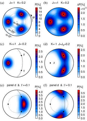
We start with the FM case . Presented Fig. 2(a) is the corresponding probability map obtained by the method of previous Sec. IV for . The probability is clearly peaked at the directions of the cubic axes attaining there the maximum value slightly less than . This is due to the cluster groundstate being a superposition of six possible classical states and a small contribution of quantum fluctuations. The width of the peaks matches well the intrinsic width estimated in Sec. IV.
That the -term favors cubic axes for the ordered moment follows also from simple analytical calculations. By treating the quantum fluctuations within second order perturbation expansion (see Ref. 28 for details), we obtain the magnetic anisotropy energy
| (7) |
depending on the moment direction given by a unit vector . This quantum correction on top of the isotropic classical energy is minimized for pointing along the cubic axes that become the easy axes, consistent with the ED result.
The case of the AF is rather different due to the presence of large quantum fluctuations already in the Heisenberg limit. This is manifested in an almost flat probability profile with of about [see Fig. 2(b)]. Nevertheless, the probability maxima again precisely locate the directions for the ordered moments, consistent with the “order-from-disorder” calculations [29; 15; 30; 28; 25] in the models containing compass- or Kitaev-type bond-directional anisotropy.
V.2 Moment direction in the zigzag phases
Having verified the method, we now move to the zigzag phases observed in Na2IrO3 and RuCl3. We first inspect the case of when the anisotropy is due to the Kitaev-term alone. Shown in Fig. 2(c) is the probability map for AF and FM , where the -axis is selected already on the classical level as discussed in Sec. III [31]. The probability is indeed strongly peaked at the direction of the -axis. The small of about is again a signature of large quantum fluctuations in the groundstate. Note that this number contains an overall reduction factor of due to the six possible zigzag states being superposed in the cluster groundstate.
The probability map Fig. 2(d) for the FM zigzag case reveals the moment being constrained to the vicinity of the -plane, as expected from classical considerations. Within this plane, the order-from-disorder mechanism selects the cubic axes and where the probability reaches its maxima. Concluding the survey of the probability maps, we show calculated including a large enough that leads to the selection of a direction within the -plane [, Fig. 2(e)] or the -axis [, Fig. 2(f)].
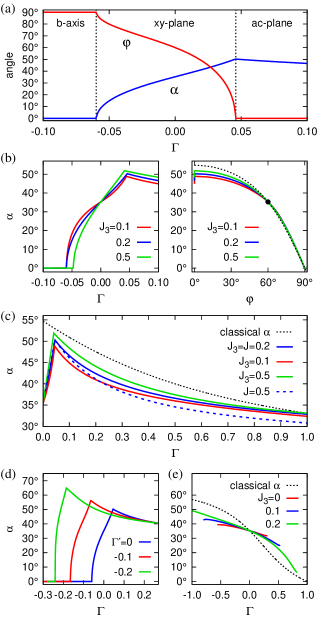
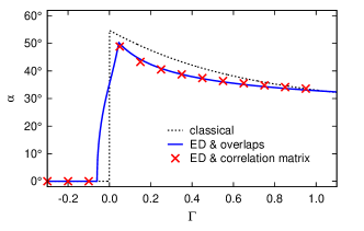
The above three examples for the FM zigzag indicate a rather complex behavior of the moments in this case, as already suggested in Fig. 1(c). In the following, we therefore focus on the full -dependence presented in Fig. 3(a) in the form of the angles (the angle to the honeycomb plane) and (polar angle of the projection into the honeycomb plane). Instead of the jump in obtained on a classical level, we find a finite window of an order-from-disorder stabilized phase, where the moment direction gradually moves from the cubic axis () to either -axis () or to the -plane (). Once the critical value of is reached, the moment either stays along the -axis or is pushed down within the -plane closer to the honeycomb plane. Fig. 3(b) illustrates the evolution of for different values of stabilizing the zigzag order. For small , the dominant directional Kitaev term makes the moment more pinned to the cubic axes, which is manifested by a significantly reduced slope of near compared to the large- case. On the other hand, the critical values of are only slightly affected by .
The above crossover behavior near may be easily understood and even semi-quantitatively reproduced by considering a competition of the classical energy and the order-from-disorder potential as follows. Keeping the moment within the -plane preferred by , we can evaluate the classical energy per site
| (8) |
In this contribution, the anisotropy is due to the - and -terms only. is complemented by an order-from-disorder potential that should contain four equivalent minima at corresponding to the cubic axes (supported by the term). Such a potential can be represented by the following form:
| (9) |
approximating by its lowest harmonic. This function is characterized by a single unknown parameter – the barrier height , determined mainly by the dominant . Assuming , the minimization of the total energy gives and the critical value . This enables us to extract effective from our numerical data. By taking observed in Fig. 3(a,b) we get . Furthermore, converting in the -plane to the angle to the honeycomb plane, we obtain “phenomenological” that roughly approximates the numerical data. The agreement between these two profiles improves with increasing , when the order-from-disorder potential becomes more harmonic and the deviation of the moment direction from the -plane for reduces [see Fig. 3(b)]. In fact, the above equations (8) and (9), together with the value of extracted from the ED data, may be used for a semi-quantitative determination of the easy axis direction within the -plane.
For curiosity, we have evaluated the potential barrier also analytically, by two slightly different methods. First, as in Sec. V.1, we estimated quantum corrections for zigzag phase along the lines of Ref. 28. This reproduced the above form (9) of the anisotropy potential, and provided a consistent estimate of . An alternative evaluation of the anisotropy potential within the linear spin-wave framework resulted in zero-point energy of the same form as (9) again, but with an overestimated value of .
In Na2IrO3 the moment direction was found [12] in the -plane suggesting that for this material. We thus focus on this particular case and investigate how the precise value of is affected by the model parameters in more detail. Already on a classical level, finite rotates the moment within the -plane from (corresponding to the -plane) toward the honeycomb plane (). Such an effect is well visible also in Fig. 3(a,b). Presented in Fig. 3(c) are a few representative curves for larger values of up to that serve as a test of the classical prediction
| (10) |
derived in Ref. 19. As we find, the quantum fluctuations included in the exact groundstate push the ordered moments much closer to the honeycomb plane. The difference is substantial and needs to be considered when trying to quantify the model parameters based on the experimental data.
So far, we have considered only, while a small negative is expected to be generated by a trigonal compression [32; 18; 19]. Based on Eq. (8), is expected to effectively shift the value of in the first approximation. Indeed, as shown in Fig. 3(d), the rough three-phase picture as in Fig. 3(a) is preserved and the negative shifts the curve in the negative direction. This enables to reach higher values, even above the -plane angle .
Finally, in Fig. 3(e) we briefly analyze the AF situation with the moment near the -axis. In contrast to the FM case, small has a relatively little effect here, because the -axis is classically selected by the dominant itself. Quantum fluctuations are found to generate an even stronger pinning to the -axis, compared to the classical solution of Ref. 19. Only a very large coupling is able to take the spin away from the -axis.
VI Comparison to experiment
VI.1 Extracting pseudospin direction from resonant x-ray and neutron scattering data
Having quantified the pseudospin easy axis direction as a function of the Hamiltonian parameters, we consider now how this “pseudomoment” direction is related to that of real magnetic moments measured by neutron and x-ray scattering experiments. To this end, we first define the pseudospin one-half wavefunctions including crystal field of trigonal symmetry. The latter splits the manifold into an orbital singlet , and the doublet . Denoting this splitting by and using the hole-representation, we have:
| (11) |
Within a point-charge model, positive (negative) would correspond to a compression (elongation) of octahedra along the trigonal -axis. The actual value of in real material is decided by various factors, but this issue is not relevant in the present context.
In terms of the effective angular momentum of the shell, state corresponds to the state, while the doublet hosts the states, using the quantization axis suggested by the trigonal crystal field. Explicitly,
| (12) | ||||
| (13) |
Via these states, pseudospin- wavefunctions are defined as:
| (14) | ||||
| (15) |
where and refer to the projections of the hole spin on the trigonal -axis. The spin-orbit “mixing” angle is given by , where .
Using the wavefunctions (14) and (15), we may express the spin and orbital moments of a hole via the pseudospin . In a cubic limit, i.e. , one has , , and total magnetic moment (note a negative -factor ). These relations imply that the pseudospin easy axis direction is identical to that of spin, orbital, and magnetic moments when trigonal field is zero. However, this is no longer valid at finite . For instance, strong compression () would completely suppress the -plane components of magnetic moments, so the pseudospin and magnetic moment will not be parallel anymore (unless pseudospin is ordered along the -axis).
The x-rays and neutrons couple initially to the spin and orbital moments, and the scattering operator has to be projected onto the pseudospin basis. We first consider an effective RXS operator. For pseudospin one-half in a trigonal field, it has to have a form , where and () is the polarization of the incoming (outgoing) photon. This can be written as , introducing a vector with . The RXS data determines a direction of this auxiliary vector ; in Na2IrO3, it was found to make an angle to the -plane [12]. However, this is not yet the pseudospin direction, since and hence , unless the trigonal field is exactly zero (unlikely in real materials). To access the pseudospin angle and quantify the model parameters, one has to know the “RXS-factors” and .
We have derived the -factors (see Appendix B for details). For the edge, they read as:
| (16) | ||||
| (17) |
Here, , , and . Fig. 4(a) shows the -factors as a function of trigonal field parameter . In cubic limit, one has hence is parallel to , as expected.
For completeness, we show also the -factors for the edge:
| (18) |
which vanish at limit, as a consequence of the spin-orbit entangled nature of pseudospins [33].
In neutron diffraction experiments, the magnetic moment is probed. For the pseudospins as defined above, the -factors are (neglecting covalency effects [7]):
| (19) | ||||
| (20) |
The -factor anisotropy can quantify the strength of the trigonal field, as illustrated in Fig. 4(b). Again, magnetic moment direction is in general different from that of pseudospin, and to access the latter one needs to know the -factors.
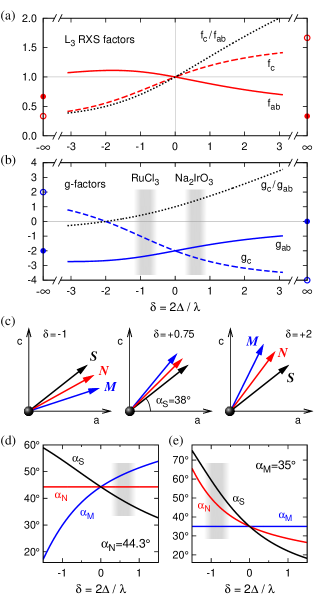
These considerations imply that the orientations of the (x-ray) vector and magnetic moment differ from each other, and also from that of pseudospin which enters the model Hamiltonian. As we show in Fig. 4(c), their relative angles come in the order for positive , and in reversed order for negative . Ideally, having measured both and directions in the same compound, one could extract the crystal field parameter using the above equations, and uniquely fix the pseudospin easy axis angle . In principle, the -factor anisotropy provides the same information on , but obtaining -factors in magnetically concentrated systems is somewhat nontrivial task. Alternatively, one could extract the value and sign of directly from the splitting and anisotropy of high-energy quartet in single crystals (see Appendix C for details).
VI.2 Implications for Na2IrO3 and RuCl3
Armed with the above relations between different moments, and using the results of Sec. V.2, let us now analyze the available experimental data on Na2IrO3 and RuCl3.
Starting with the case of Na2IrO3, we utilize the value determined recently by RXS [12]. Keeping this experimental constraint, in Fig. 4(d) we plot the remaining angles and as functions of the relative strength of the trigonal crystal field . In Ref. 19, the value was deduced based on the splitting of quartet [37]. As seen in Fig. 4(b), the corresponding is also roughly consistent with the anisotropy of the -factors, , obtained by fitting the temperature-dependent magnetic susceptibilities [36]. The data in Fig. 4(d) then suggests that the magnetic moment takes an angle of about to the honeycomb plane, while the pseudospin angle is roughly . Such a deviation of the pseudospin from the -plane () implies a sizable value. Based on Fig. 3(c) we may naively expect the ratio in the range . We emphasize, however, that this conclusion relies on the above estimate of the trigonal field, that should be verified by measuring the “magnetic” angle directly by neutron scattering.
Compared to Na2IrO3, RuCl3 shows an opposite magnetic anisotropy behavior with [34]. The magnetic structure has been recently investigated by neutron scattering [38], with the result and being equal to either or . Similarly to Fig. 4(d), in Fig. 4(e) we keep the measured angle, now , fixed at its experimental value, and plot and for varying . This parameter could be obtained from the anisotropy of transitions in single crystals (see Appendix C). We are not aware of such a direct measurement in RuCl3, so the trigonal field is best assessed by considering the anisotropy of the -factors. Refs. 34; 35 reported in-plane and out-of-plane magnetization curves measured for high fields up to . Even though the saturation was not reached, the data indicate the value . A similar ratio was also found by Yadav et al. [39] using quantum chemistry methods and by fitting the high-field data of Ref. 35. The corresponding puts the pseudospin angle at relatively high values of about [see Fig. 4(e)]. Adopting this estimate, we will try to identify a consistent parameter window.
Unfortunately, the present neutron experiment [38] could not directly resolve the orientation of the moments with respect to the -axis, i.e. whether or . The absence of this most conclusive evidence for the sign of the Kitaev interaction requires us to consider both possibilities.
We assume first FM as obtained in two recent ab-initio calculations of the exchange interactions in RuCl3 [24; 39]. Fig. 3(c) gives a hint that the estimated can be reached for small only. As seen in Fig. 3(d), by including small negative that shifts the crossover towards negative , the pseudospin direction may rotate even far above the -plane. Interestingly, the corresponding parameter regime matches well the prediction by quantum chemistry calculations [39].
Now we analyze the AF case, proposed for RuCl3 in Refs. 40; 38; 13. In this case, the zigzag order is obtained on the level of the two-parameter Kitaev-Heisenberg model [20] alone, and this simplicity makes the AF scenario particularly attractive. In the zigzag phase of the two-parameter model, the pseudospins point along the cubic -axis leading to . This can be reconciled with the experimental value only in a nearly cubic situation with a small trigonal distortion. Considering however the large anisotropy of the -factors discussed above and the resulting , it seems that the AF Kitaev interaction needs to be supplemented by other anisotropic interactions lifting the pseudospin considerably up. This scenario is addressed in Fig. 3(e). We have found, that does not influence much so that we focus on the -dependence. Since the AF zigzag phase becomes fragile if the other anisotropy terms are included, the model has to be additionally extended by . Based on the data of Fig. 3(e), we may conclude that large negative comparable to is needed to obtain . It should be carefully checked if such a substantially extended model is still consistent with other experimental data, in particular with the spin excitation spectrum with small only gaps [13].
We would like to stress again, that our analysis of RuCl3 for both and heavily relied on the relative trigonal field strength inferred solely from the magnetization anisotropy in high magnetic fields. It is thus highly desirable to measure the complementary angle by RXS and quantify more precisely, as suggested in the previous subsection. As discussed in Appendix C, measuring the anisotropy of states by inelastic neutron scattering in single crystals would be also very helpful.
To summarize this section, in Na2IrO3, the measured moment direction [12] with well fixes the FM sign of the Kitaev interaction, and our analysis of its angle from the -plane suggests that coupling is present. Concerning RuCl3, the current ambiguity in the angle ( or ) leaves open the issue of the sign of . There is also an uncertainty in the trigonal field value ; based so far on the -factor anisotropy, we found that FM with relatively small , values would be consistent with the data, while AF situation requires large couplings comparable to .
VII Conclusions
We have investigated the ordered moment direction in the zigzag phases of the extended Kitaev-Heisenberg model for honeycomb lattice magnets. Our method analyzes the exact cluster groundstates using a particular set of spin coherent states and as such fully accounts for the quantum fluctuations. The interplay among the various anisotropic interactions leads to a complex behavior of the ordered moment direction as a function of the model parameters. We have found substantial corrections to the results of a classical analysis that are important when quantifying the exchange interactions based on the experimental data.
We have pointed out that, away from the ideal cubic situation, the notion of the “ordered moment direction” has to be precisely specified. Assuming a trigonal field relevant to the layered honeycomb systems, we have derived relations among the directions of (i) the pseudospins entering the model Hamiltonian, (ii) the magnetic moments measured by neutron diffraction, and (iii) the moment direction as probed by resonant magnetic x-ray scattering. These relations and a combination of neutron and x-ray data should enable a reliable quantification of the trigonal field as well as the pseudospin direction in future experiments.
Using the above results, we have analyzed the currently available experimental data on Na2IrO3 and RuCl3 and identified plausible parameter regimes in these compounds.
Acknowledgements.
We would like to thank G. Jackeli, B.J. Kim, S.E. Nagler, and J. Rusnačko for helpful discussions. JC acknowledges support by Czech Science Foundation (GAČR) under project no. GJ15-14523Y and MŠMT ČR under NPU II project CEITEC 2020 (LQ1601).Appendix A Comparison of numerical methods
As mentioned in the main text, the standard method to obtain the ordered moment direction using the ED groundstate is to evaluate the spin-spin correlation matrix () at the ordering vector and to find its eigenvector corresponding to the largest eigenvalue. However, there are two main problems associated with this simple method, both emerging since the cluster groundstate is a linear superposition of degenerate orderings where the individual orderings have equal weights:
(i) If there are several equivalent easy axis directions associated with the selected ordering vector , they will be characterized by the same eigenvalue. This leads to a degenerate eigenspace and prevents us to resolve such directions. The most severe cases are those with a dominant Heisenberg interaction presented in Fig. 2(a,b). Here we have three degenerate easy axes , , which makes the correlation matrix proportional to a unit matrix and thus isotropic. In the FM zigzag situation shown in Fig. 2(d) and the entire middle phase in Fig. 3(a), two degenerate moment directions for a particular zigzag pattern (selected by ) are possible and the correlation matrix therefore just uncovers the softness of the -plane. Only after these two directions merge a for large enough , the moment direction can be identified.
(ii) The zigzag pattern to be probed is selected by choosing the ordering vector . In contrast to an infinite lattice, at a finite cluster this separation of the three zigzag directions is not perfect. The range of spin correlations is limited by the size of the cluster and the corresponding momentum space peaks become broad. The correlation matrix at given is thus “polluted” by small contributions of the two other zigzags in the groundstate, that are associated with the remaining ordering vectors.
Our method introduced in Sec. IV does not suffer from the above problems and is able to handle all the situations encountered. This is due to the full resolution of the various degenerate orderings present in the cluster groundstate by using a prescribed ordering pattern and by a construction of a full directional map.
Appendix B Derivation of the L-edge RXS operator
Resonant x-ray scattering is conceptually similar to the Raman light scattering, in a sense that both processes involve the intermediate states created and subsequently eliminated by incoming and outgoing photons. However, the nature of the intermediate states in these two cases is radically different: while the Raman light scattering involves intersite transitions, the x-rays create the high-energy on-site transitions. As a result, the Raman light scattering probes intersite (two-magnon) spin flips, while the presence of strong spin-orbit coupled -core hole in the RXS intermediate states makes a single-ion spin flips a dominant magnetic scattering channel (see the recent review [41] and references therein for details).
A complex time-dynamics of the intermediate states makes the x-ray scattering process hard to analyze microscopically. However, as far as one is concerned with the low-energy excitations in Mott insulators, the problem of the intermediate states can be disentangled and cast in the form of frequency independent phenomenological constants [42; 43; 44]. This results is an effective RXS operator formulated in terms of low-energy (orbital, spin, …) degrees of freedom alone. The form of this operator is dictated by symmetry. In essence, this approach is similar to that of Fleury and Loudon [45] widely used in the theories of Raman light scattering in quantum magnets.
While the RXS operator used in the main text follows from an underlying trigonal symmetry, the ratio between and constants requires specific calculations. This can be easily done, with some routine modifications of the previous work for the case of tetragonal symmetry [46; 47], as outlined below.
In cubic axes (see Fig. 1), a dipolar to transition operator reads as:
| (21) |
where are the polarization factors, and , , . Here and below, it is implied that and operators carry also the spin quantum numbers (, ) over which summation is taken.
In the quantization axes , suggested by the trigonal crystal field, this operator takes the following form:
| (22) |
where
| (23) |
Here, the indices and stand for the orbital quantum numbers of and electrons.
Within the above Fleury-Loudon-like approach to the x-ray scattering problem, effective RXS operator is given by , and its part responsible for the magnetic scattering reads as .
Next, the core-hole operators in (23) are expressed in terms of spin-orbit split and eigenstates of the level, resulting in two sets of operators active in and edges, correspondingly. After “integrating out” these and operators, the product becomes a simple quadratic form of operators. Finally, projecting this form onto a pseudospin doublet (given by Eqs. 14 and 15 of the main text), we arrive at the RXS operator , with the -factors shown in the main text. Via the pseudospin wavefunctions, the RXS -factors are sensitive to a trigonal field strength.
Appendix C Determination of the trigonal field from magnetic excitation spectra
Under spin-orbit coupling and trigonal crystal field , -hole states split into three levels , , and , see Fig. 6(a). The level hosts a Kramers pseudospin one-half (corresponding to in the cubic limit), with the wavefunctions
| (24) | ||||
| (25) |
as were given by Eqs. 14 and 15 of the main text. The upper Kramers doublets and are derived from spin-orbit quartet. The former correspond to pure states of moment:
| (26) | ||||
| (27) |
while the level wavefunctions are given by
| (28) | ||||
| (29) |
corresponding to states of quartet in the cubic limit, and containing some admixture of the original doublet at finite . The energies of these states are: and .
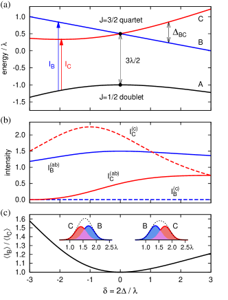
Transitions from the ground state level to and states are magnetically active; their spectral weights in the dynamical spin structure factor are determined by matrix elements of the magnetic moment :
| (30) | ||||
| (31) |
Out-of-plane moment matrix elements between and vanish (independent of the spin-orbit mixing angle ), while
| (32) |
In the magnetic excitation spectra, a transition gives a peak at the energy
| (33) |
with the following intensities for different components of the dynamical spin structure factor
| (34) |
The second transition is peaked at the energy
| (35) |
and has the intensity
| (36) |
The and peaks are separated by ; at small trigonal splitting , this can be approximated as . At positive (negative) , the peak position is lower (higher) than that of peak, see Fig. 6(a).
Fig. 6(b) shows that the intensities of both transitions are highly anisotropic with respect to -plane and -axis polarizations, with the opposite behavior of and contributions. The out-of-plane response is due to the transition exclusively, while peak dominates the -plane intensity. This should enable to distinguish them and determine thereby both the sign and value of trigonal field parameter from a single-crystal, spin-polarized neutron scattering data.
On the other hand, the powder averaged intensities of and peaks are nearly the same for realistic values of , see Fig. 6(c). Even at , the two peaks may overlap to give a single broad line, leaving an ambiguity in the sign of parameter .
References
- [1] N.F. Mott, Metal-Insulator Transitions (Taylor and Francis, London, 1974).
- [2] M. Imada, A. Fujimori, and Y. Tokura, Rev. Mod. Phys. 70, 1039 (1998).
- [3] J.B. Goodenough, Magnetism and the Chemical Bond (Interscience Publ., New York, 1963).
- [4] K.I. Kugel and D.I. Khomskii, Sov. Phys. Usp. 25, 231 (1982).
- [5] G. Khaliullin and S. Maekawa, Phys. Rev. Lett. 85, 3950 (2000).
- [6] G. Khaliullin, Prog. Theor. Phys. Suppl. 160, 155 (2005).
- [7] A. Abragam and B. Bleaney, Electron Paramagnetic Resonance of Transition Ions (Clarendon Press, Oxford, 1970).
- [8] G. Khaliullin, W. Koshibae, and S. Maekawa, Phys. Rev. Lett. 93, 176401 (2004).
- [9] G. Jackeli and G. Khaliullin, Phys. Rev. Lett. 102, 017205 (2009).
- [10] A. Kitaev, Ann. Phys. 321, 2 (2006).
- [11] J.G. Rau, E.K.-H. Lee, and H.-Y. Kee, Annu. Rev. Condens. Matter Phys. 7, 195 (2016).
- [12] S.H. Chun, J.-W. Kim, Jungho Kim, H. Zheng, C.C. Stoumpos, C.D. Malliakas, J.F. Mitchell, K. Mehlawat, Y. Singh, Y. Choi, T. Gog, A. Al-Zein, M. Moretti Sala, M. Krisch, J. Chaloupka, G. Jackeli, G. Khaliullin, and B.J. Kim, Nature Phys. 11, 462 (2015).
- [13] A. Banerjee, C.A. Bridges, J.-Q. Yan, A.A. Aczel, L. Li, M.B. Stone, G.E. Granroth, M.D. Lumsden, Y. Yiu, J. Knolle, S. Bhattacharjee, D.L. Kovrizhin, R. Moessner, D.A. Tennant, D.G. Mandrus, and S.E. Nagler, Nature Mater. 15, 733 (2016).
- [14] K.W. Plumb, J.P. Clancy, L.J. Sandilands, V.V. Shankar, Y.F. Hu, K.S. Burch, H.-Y. Kee, and Y.-J. Kim, Phys. Rev. B 90, 041112(R) (2014).
- [15] J. Chaloupka, G. Jackeli, and G. Khaliullin, Phys. Rev. Lett. 105, 027204 (2010).
- [16] V.M. Katukuri, S. Nishimoto, V. Yushankhai, A. Stoyanova, H. Kandpal, S. Choi, R. Coldea, I. Rousochatzakis, L. Hozoi, and J. van den Brink, New J. Phys. 16, 013056 (2014).
- [17] J.G. Rau, E.K.-H. Lee, and H.-Y. Kee, Phys. Rev. Lett. 112, 077204 (2014).
- [18] J.G. Rau and H.-Y. Kee, ArXiv e-prints (2014), arXiv:1408.4811 [cond-mat.str-el].
- [19] J. Chaloupka and G. Khaliullin, Phys. Rev. B 92, 024413 (2015).
- [20] J. Chaloupka, G. Jackeli, and G. Khaliullin, Phys. Rev. Lett. 110, 097204 (2013).
- [21] I. Kimchi and Y.-Z. You, Phys. Rev. B 84, 180407(R) (2011).
- [22] S.K. Choi, R. Coldea, A.N. Kolmogorov, T. Lancaster, I.I. Mazin, S.J. Blundell, P.G. Radaelli, Y. Singh, P. Gegenwart, K.R. Choi, S.-W. Cheong, P.J. Baker, C. Stock, and J. Taylor, Phys. Rev. Lett. 108, 127204 (2012).
- [23] Y. Yamaji, Y. Nomura, M. Kurita, R. Arita, and M. Imada, Phys. Rev. Lett. 113, 107201 (2014).
- [24] S.M. Winter, Y. Li, H.O. Jeschke, and R. Valentí, Phys. Rev. B 93, 214431 (2016).
- [25] Y. Sizyuk, P. Wölfle, and N.B. Perkins, ArXiv e-prints (2016), arXiv:1603.06487 [cond-mat.str-el].
- [26] A. Auerbach, Interacting Electrons and Quantum Magnetism (Springer, New York, 1994).
- [27] For a discussion of the order-from-disorder phenomena in frustrated spin systems, see A.M. Tsvelik, Quantum Field Theory in Condensed Matter Physics (Cambridge University Press, Cambridge, 1995), Chap. 17, and references therein.
- [28] G. Jackeli and A. Avella, Phys. Rev. B 92, 184416 (2015).
- [29] G. Khaliullin, Phys. Rev. B 64, 212405 (2001).
- [30] Z. Nussinov and J. van den Brink, Rev. Mod. Phys. 87, 1 (2015).
- [31] However, the separation of the individual zigzag chain directions is an order-from-disorder effect, since a linear combination of different zigzag patterns is a classical groundstate as well.
- [32] S. Bhattacharjee, S.-S. Lee, and Y.B. Kim, New J. Phys. 14, 073015 (2012).
- [33] B.J. Kim, H. Ohsumi, T. Komesu, S. Sakai, T. Morita, H. Takagi, and T. Arima, Science 323, 1329 (2009).
- [34] Y. Kubota, H. Tanaka, T. Ono, Y. Narumi, and K. Kindo, Phys. Rev. B 91, 094422 (2015).
- [35] R.D. Johnson, S.C. Williams, A.A. Haghighirad, J. Singleton, V. Zapf, P. Manuel, I.I. Mazin, Y. Li, H.O. Jeschke, R. Valentí, and R. Coldea, Phys. Rev. B 92, 235119 (2015).
- [36] Y. Singh and P. Gegenwart, Phys. Rev. B 82, 064412 (2010).
- [37] H. Gretarsson, J.P. Clancy, X. Liu, J.P. Hill, E. Bozin, Y. Singh, S. Manni, P. Gegenwart, J. Kim, A.H. Said, D. Casa, T. Gog, M.H. Upton, H.-S. Kim, J. Yu, V.M. Katukuri, L. Hozoi, J. van den Brink, and Y.-J. Kim, Phys. Rev. Lett. 110, 076402 (2013).
- [38] H.B. Cao, A. Banerjee, J.-Q. Yan, C.A. Bridges, M.D. Lumsden, D.G. Mandrus, D.A. Tennant, B.C. Chakoumakos, and S.E. Nagler, Phys. Rev. B 93, 134423 (2016).
- [39] R. Yadav, N.A. Bogdanov, V.M. Katukuri, S. Nishimoto, J. van den Brink, and L. Hozoi, ArXiv e-prints (2016), arXiv:1604.04755 [cond-mat.str-el].
- [40] H.-S. Kim, V. Shankar, A. Catuneanu, and H.-Y. Kee, Phys. Rev. B 91, 241110 (2015).
- [41] L.J.P. Ament, M. van Veenendaal, T.P. Deveraux, J.P. Hill, and J. van den Brink, Rev. Mod. Phys. 83, 705 (2011).
- [42] L.J.P. Ament and G. Khaliullin, Phys. Rev. B 81, 125118 (2010).
- [43] M.W. Haverkort, Phys. Rev. Lett. 105, 167404 (2010).
- [44] L. Savary and T. Senthil, ArXiv e-prints (2015), arXiv:1506.04752 [cond-mat.str-el].
- [45] P.A. Fleury and R. Loudon, Phys. Rev. 166, 514 (1968).
- [46] L.J.P. Ament, G. Khaliullin, and J. van den Brink, Phys. Rev. B 84, 020403(R) (2011).
- [47] J. Kim, D. Casa, M.H. Upton, T. Gog, Y.-J. Kim, J.F. Mitchell, M. van Veenendaal, M. Daghofer, J. van den Brink, G. Khaliullin, and B.J. Kim, Phys. Rev. Lett. 108, 177003 (2012).