Sparse Estimation of Generalized Linear Models (GLM)
via Approximated Information Criteria

Abstract

We propose a new sparse estimation method, termed MIC (Minimum approximated Information Criterion), for generalized linear models (GLM) in fixed dimensions. What is essentially involved in MIC is the approximation of the $\ell_{0}$-norm with a continuous unit dent function. Besides, a reparameterization step is devised to enforce sparsity in parameter estimates while maintaining the smoothness of the objective function. MIC yields superior performance in sparse estimation by optimizing the approximated information criterion without reducing the search space and is computationally advantageous since no selection of tuning parameters is required. Moreover, the reparameterization tactic leads to valid significance testing results that are free of post-selection inference. We explore the asymptotic properties of MIC and illustrate its usage with both simulated experiments and empirical examples.

Key Words:  BIC; Generalized linear models; Post-selection inference; Sparse estimation; Regularization; Variable selection

1 Introduction

Suppose that data $\mathcal{L}:=\{(y_{i},\mathbf{x}_{i}):i=1,\ldots,n\}$ consist of $n$ i.i.d. copies of $\{y,\mathbf{x}\}$, where $y$ is the response variable and $\mathbf{x}=(x_{1},\ldots,x_{p})^{T}\in\mathbb{R}^{p}$ is the predictor vector. WLOG, we assume that the $x_{ij}$’s are standardized throughout the paper. Consider the regression models that link the mean response $y$ and covariates $\mathbf{x}$ through its linear predictor $\mathbf{x}^{T}\mbox{\boldmath$\beta$}$ with $\mbox{\boldmath$\beta$}=(\beta_{1},\ldots,\beta_{p})^{T}$, e.g., generalized linear models (GLM; McCullagh and Nelder, 1989). Concerning variable selection, the true $\beta$ is often sparse in the sense that some of its components are zeros. To this end, we assume that either there is no nuisance parameter involved or the nuisance parameters and $\beta$ are orthogonal (Cox and Reid, 1987). Hence we simply denote the log-likelihood function as $L(\mbox{\boldmath$\beta$})=\sum_{i=1}^{n}\log f(y_{i};\mathbf{x}_{i},\mbox{\boldmath$\beta$}).$

A classical variable selection procedure is the best subset selection (BSS), and two commonly-used information criteria are AIC (Akaike, 1974) and BIC (Schwarz, 1978). BSS can be formulated as

$$\min_{\mbox{\boldmath$\beta$}\,\in\,\Omega}~{}~{}-2\cdot L(\mbox{\boldmath$\beta$})+\lambda_{0}\cdot\parallel\mbox{\boldmath$\beta$}\parallel_{0},$$ (1.1)

where the penalty parameter $\lambda_{0}$ is fixed as 2 in AIC or $\ln(n)$ in BIC. We shall focus more on the use of BIC for its superior empirical performance in variable selection widely reported in the literature. In addition, the ‘$\ell_{0}$-norm’ $\parallel\mbox{\boldmath$\beta$}\parallel_{0}=\mbox{card}(\mbox{\boldmath$\beta$})=\sum_{j=1}^{p}I(\beta_{j}\neq 0)$ denotes the cardinality or the number of nonzero components in $\beta$ and the search space in (1.1) is the entire parameter space $\Omega$ for $\mbox{\boldmath$\beta$}.$ Due to the discrete nature of cardinality, $\Omega$ consists of $\beta$ associated with all possible $2^{p}$ sparsity structures. Optimization of (1.1) proceeds in two steps: first maximize the log-likelihood function for every known sparsity structure in $\beta$ and then compare the resulting information criteria $-2\cdot L(\widehat{}\mbox{\boldmath$\beta$})+\lambda_{0}\cdot\parallel\widehat{}\mbox{\boldmath$\beta$}\parallel_{0}$ across all model choices, where $\widehat{}\mbox{\boldmath$\beta$}$ denotes the maximum likelihood estimator of $\beta$ and hence $L(\widehat{}\mbox{\boldmath$\beta$})$ corresponds to the maximized log-likelihood function. While faster algorithms (Furnival and Wilson, 1974) are available, solving (1.1) is non-convex and NP-hard. As a result, the best subset selection becomes infeasible when $p$ is moderately large.

Both ridge regression (Hoerl and Kennard, 1970) and LASSO (Tibshirani, 1996) were proposed as convex relaxations of (1.1). Their general form is given by

$$\min_{\mbox{\boldmath$\beta$}}~{}-2\cdot L(\mbox{\boldmath$\beta$})+\lambda\,\cdot\parallel\mbox{\boldmath$\beta$}\parallel_{r},$$ (1.2)

where $\parallel\mbox{\boldmath$\beta$}\parallel_{r}=\sum_{j=1}^{p}|\beta_{j}|^{r}$ for some $r>0$. To assure convexity, $r\geq 1$ is typically considered, and $r=1$ and $r=2$ result in LASSO and ridge regression, respectively. While both methods provide a continuous regularization process for ill-posed estimation problems, LASSO enjoys the additional property of enforcing sparsity. Its regularization path is shown to be piecewise-linear and can be efficiently computed via either the homotopy algorithm (Osborne, Presnell, and Turlach, 2000 and and Efron et al., 2004) or the coordinate descent (Fu, 1998 and Friedman, Hastie, and Tibshirani, 2010). Since the proposal of LASSO, a vast statistical literature has been devoted to the study of $\ell_{1}$ regularization, and numerous variants have been developed for enhancement and expansion. An up-to-date literature review can be found in Zhang (2010), Breheny and Huang (2011), Shen, Pan, and Zhu (2012) and references therein.

However, the convex relaxation methods with $\parallel\mbox{\boldmath$\beta$}\parallel_{r}$ are mainly motivated by optimization theory; by no means are they intended as an approximation of $\parallel\mbox{\boldmath$\beta$}\parallel_{0}$ in (1.1). With the formulation (1.2), one would lose track of $\lambda_{0}$. As a result, $\lambda$ in (1.2) becomes a tuning parameter and its choice has to be selected with extra efforts. The common practice of regularization involves two steps as well: first compute the whole regularization path, i.e., the solution of $\beta$ for every tuning parameter $\lambda\geq 0$, and then tune for the best $\lambda^{\star}$ via some criterion such as cross validation or BIC (see, e.g., Wang, Li, and Tsai, 2007). This practice amounts to first reducing the search space from the $p$-dimensional $\Omega$ to a one-dimensional curve (often termed as regularization path) $\{\widehat{\mbox{\boldmath$\beta$}}(\lambda):\lambda\geq 0\}$, and subsequently selecting the best estimator $\widehat{\mbox{\boldmath$\beta$}}(\lambda^{\star})$. To have correct variable selection, it is essential that the true sparsity structure be included in the much reduced search space, i.e., the regularization path. However, this requirement cannot be guaranteed for many existing $\ell_{1}$ regularization methods. In particular, selection consistency of LASSO entails a strong irrepresentable assumption (Zhao and Yu, 2006). This has motivated the proposals of non-convex penalties such as SCAD (Fan and Li, 2001) and MCP (Zhang, 2010). Another statistically awkward issue with regularization is the selection of the tuning parameter, which is conventional in optimization. Selecting of the best tuning parameter $\hat{\lambda}$ is computationally costly. Moreover, even though $\hat{\lambda}$ is clearly a statistics, selection of the tuning parameter is never treated as a statistical estimation problem and no statistical inference is routinely done for unknown reasons, at least in the frequentist’s approach.

Another inherent problem with both BSS and regularization is the post-selection inference. Conventional statistical inference is made on the final model with selected variables or nonzero coefficients by ignoring the effect of model selection, which can be problematic as pointed out by Leeb and Pötscher (2005) among others. One evidence is that no statistical inference is available for parameters associated with those unselected variables in BSS or zero estimates in regularization. How to make valid post-selection inference is currently under intensive statistical research. See, e.g., Berk et al. (2013), Efron (2014), and Lockhart et al. (2014).

In this article, we propose a new sparse estimation method for GLM, termed Minimum approximated Information Criterion (MIC). The main idea is to reformulate the problem by approximating the $\ell_{0}$ norm in (1.1) with a continuous function. This leads to a smoothed version of BIC that can be directly optimized. We then devise a reparameterization step that helps enforce sparsity in parameter estimates while maintaining smoothness of the objective function at the same time. The formulation results in a non-convex yet smooth programming problem. This setup allows us to borrow strength from established methods and theories in both optimization and statistical estimation. Many available smooth optimization algorithms can be conveniently used to solve MIC. At the same time, the smoothness of the estimating equation allows us to derive valid significance testings on parameters that are free of post-selection inference.

Our proposed MIC method combines model selection and parameter estimation together under the common framework of optimization and accomplishes both within one single step. Compared to many currently available methods, it offers the three major advantages. First, MIC yields the best performance to date in sparse estimation with fixed dimensions because it seeks optimization of BIC, albeit approximated, without reducing the search space. Secondly, MIC is computationally advantageous by avoiding selection of the tuning parameters. Thirdly, MIC makes available inference results for both zero and non-zero coefficient estimates via the reparameterization trick. MIC was first proposed by Su (2015) in linear regression with focus on variable selection only.

We emphasize again all our discussions are restricted to fixed dimensions. The remainder of this article is organized as follows. Section 2 presents the MIC method in detail. In Section 3, we explore its asymptotic properties under regular conditions. Section 4 presents simulation studies and data analysis examples. Section 5 ends the article with a brief discussion.

2 Minimizing the Approximated BIC

Our proposed method conducts sparse estimation of GLM by minimizing an approximated Bayesian information criterion. In its final form, MIC simply solves the following unconstrained smooth optimization problem:

$$\min_{\displaystyle\mbox{\boldmath$\gamma$}}~{}~{}~{}-2\,L(\mathbf{W}\mbox{\boldmath$\gamma$})~{}+~{}\log(n)\cdot\mbox{tr}(\mathbf{W}),$$ (2.1)

where $\mbox{\boldmath$\beta$}=\mathbf{W}\mbox{\boldmath$\gamma$}$ and $\mathbf{W}=\mbox{diag}\left(w_{j}\right)$ with $w_{j}=w(\gamma_{j})=\tanh(a\,\gamma_{j}^{2})$ for $j=1,\ldots,p.$ The formulation of (2.1) involves a nonnegative parameters $a$, which controls the sharpness of approximation. Although asymptotic results suggest $a=O(n)$, the empirical performance of MIC is rather stable with respect to the choice of $a$. Thus $a$ will be fixed a priori.

The MIC method in (2.1) can be described in two steps: (i.) approximating cardinality with a unit dent function and (ii.) achieving sparsity with reparameterization. We shall explain the detailed procedure step-by-step in the ensuing subsections.

2.1 Unit Dent Functions

First of all, we seek an approximation to the cardinality in (1.1) with a continuous or smooth surrogate function $w(\cdot)$. This will make the discrete optimization problem in (1.1) continuous. For the convenience of presentation, we shall use $\beta$ as a generic notation for $\beta_{j}$ from time to time. The cardinality of $\beta$ is $\sum I\{\beta_{j}\neq 0\}$ and hence it reduces to approximating the indicator function $I\{\beta\neq 0\}.$ To this end, a suitable surrogate function $w(\beta)$ must be a unit dent function, as defined below.

Definition.

Denote $\bar{\mathbb{R}}=R\cup\{-\infty,\infty\}$. A unit dent function is a continuous function $w:\bar{\mathbb{R}}\rightarrow[0,1]$ that satisfies the following properties:

1. $w(\cdot)$ is an even function such that $w(\beta)=w(-\beta);$

2. $w(0)=0$ and $\lim_{\beta\rightarrow\infty}w(\beta)=1$;

3. $w(\beta)$ is increasing on $\mathbb{R}_{+}$.

The above definition implies that $w(\beta)$ is decreasing on $\mathbb{R}_{-}$ and $\lim_{\beta\rightarrow-\infty}w(\beta)=1.$ If $w(\beta)$ is differentiable, then $\dot{w}(\beta)\geq 0$ on $\mathbb{R}+$ and $\dot{w}(\beta)\leq 0$ on $\mathbb{R}_{-}$. The $[0,1]$ range requirement essentially makes $w(\cdot)$ non-convex, but this is necessary in order for $\sum w(\beta)$ to approximate cardinality, namely, $\parallel\!\mbox{\boldmath$\beta$}\!\parallel_{0}\approx\,\sum_{j=1}^{p}w(\beta_{j}).$ In addition, the condition $\lim_{|\beta|\rightarrow\infty}w(\beta)=1$ implies that $w(\beta)$ is approximately a constant function and hence $\dot{w}(\beta)=0$ for large $\beta$. As a consequence, when used as a penalty function, $w(\beta)$ essentially does not alter the related normal equations or score equations. Motivated by bump functions, we name $w(\cdot)$ a ‘dent’ function. A special family of bump functions, called mollifiers, are known as smooth approximations to the identity (Friedrichs, 1944). If a mollifier $\phi(\cdot)$ is normalized to have the range $[0,1]$, then $1-\phi(\cdot)$ is a unit dent function.

Let $\mathcal{D}$ denote the family of all unit dent functions. It can be easily seen that $\mathcal{D}$ is closed under operations such as composition and product. In particular, it is closed under power transformation. Namely, if $w(\beta)\in\mathcal{D}$, then $w^{k}(\beta)\in\mathcal{D}$ for $k\in\mathbb{N}$. It is worth noting that unit dent functions have appeared in the regularization literature. These include the truncated $\ell_{r}$ penalty studied by Shen, Pan, and Zhu (2012). The penalty functions SCAD (Fan and Li, 2001) and MCP (Zhang, 2010) can also be modified into unit dent functions. See Figure 1 for graphical illustrations of a number of unit dent functions.

To enforce sparsity, it is necessary for the penalty function to be non-smooth with a singularity at $\beta=0$, as indicated by Fan and Li (2001). In our proposal, however, we advocate the use of smooth unit dent functions. The primary reason is that we want the proposed method to be a natural extension of maximum likelihood estimation. Since most likelihood or log-likelihood functions are smooth, we do not want to alter this nature. Furthermore, the smoothness property allows us to capitalize on well-developed theories and methods in both optimization and statistical inference. Our approach is to have smooth penalty functions and achieve sparsity in a different way.

While many smooth unit dent functions can be considered, we shall mainly focuses on the hyperbolic tangent function,

$$w(\beta)\,=\,\tanh(a\beta^{2})\,=\,\frac{\exp(2a\beta^{2})-1}{\exp(\displaystyle 2a\beta^{2})+1}\,=\,2\,\mbox{logistic}(2a\beta^{2})-1.$$ (2.2)

Figure 1: Several unit dent functions for approximating $I(\beta\neq 0).$ (a) Truncated $L_{r}$: $w(\beta;a,r)=\left(|\beta|/a\right)^{r}$ if $|\beta|\leq a$ and 1 otherwise; (b) modified SCAD: $w(\beta;a)=a|\beta|$ if $|\beta|\leq a$; $\{2a(2-a^{2})|\beta|-a^{4}-a^{2}\beta^{2}\}/\{4(1-a^{2})\}$ if $a<|\beta|<(2-a^{2})/a$; and 1 if $|\beta|>(2-a^{2})/a$ for $0<a<\sqrt{2/3}$; (c) modified MCP: $w(\beta;a)=a|\beta|-a^{2}\beta^{2}/4$ if $|\beta|\leq 2/a$ and 1 if $|\beta|>2/a$ for $0<a<\sqrt{2}$; (d) hyperbolic tangent $w(\beta;a)=\tanh(a\cdot\beta^{2});$ (e) Weight Elimination (WE); (f) Converse Mollifier (CM) $w(\beta)=1-\exp\left\{-\beta^{2}/(b^{2}-\beta^{2})\right\}\cdot I\left\{|\beta|\leq b\right\}$ for $b>0$.

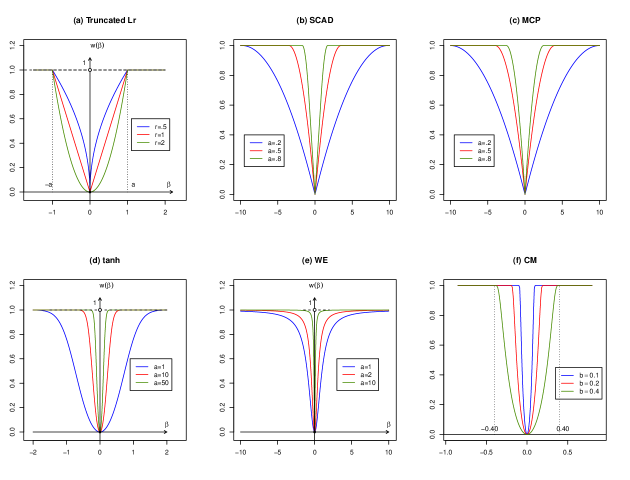
This is because its derivatives are easily calculated, with the first two given by $\dot{w}(\beta)~{}=~{}2a\beta(1-w^{2})$ and $\ddot{w}(\beta)~{}=~{}2a(1-w^{2})(1-4a\beta^{2}w).$ In addition, the $\tanh(\cdot)$ function is associated with the logistic or expit function which is widely used in statistics. A plot of $w(\beta)$ versus $\beta$ for different $a$ values is provided in Figure 1(d). It can be seen that a larger $a$ yields a sharper approximation to the indicator function $I\{\beta\neq 0\}.$

With the surrogate function $w(\beta)=\tanh(a\beta^{2})$, we seek to solve

$$\min_{\mbox{\boldmath$\beta$}}~{}~{}-2\cdot L(\mbox{\boldmath$\beta$})+\lambda_{0}\cdot\sum_{j=1}^{p}w(\beta_{j}).$$ (2.3)

Expanding $L(\mbox{\boldmath$\beta$})$ at the MLE $\widehat{\mbox{\boldmath$\beta$}}$ and then using the fact that $\nabla L(\widehat{\mbox{\boldmath$\beta$}})=\mathbf{0}$, we have

$$L(\mbox{\boldmath$\beta$})\,\approx\,L(\widehat{\mbox{\boldmath$\beta$}})+(\mbox{\boldmath$\beta$}-\widehat{\mbox{\boldmath$\beta$}})^{T}\left\{\nabla^{2}L(\widehat{\mbox{\boldmath$\beta$}})/2\right\}(\mbox{\boldmath$\beta$}-\widehat{\mbox{\boldmath$\beta$}}),$$

where $\nabla L(\widehat{\mbox{\boldmath$\beta$}})$ and $\nabla^{2}L(\widehat{\mbox{\boldmath$\beta$}})$ are the gradient vector and Hessian matrix of $L(\mbox{\boldmath$\beta$})$ evaluated at $\widehat{\mbox{\boldmath$\beta$}}$, respectively. Thus, the penalized optimization form in (2.3) can be viewed as the Lagrangian that roughly corresponds to a constrained optimization problem:

$$\min_{\mbox{\boldmath$\beta$}}~{}~{}(\mbox{\boldmath$\beta$}-\widehat{\mbox{\boldmath$\beta$}})^{T}\left\{-\,\nabla^{2}L(\widehat{\mbox{\boldmath$\beta$}})\right\}(\mbox{\boldmath$\beta$}-\widehat{\mbox{\boldmath$\beta$}})\mbox{~{}~{}subject to~{}~{}}\sum_{j=1}^{p}w(\beta_{j})\leq t_{0},$$ (2.4)

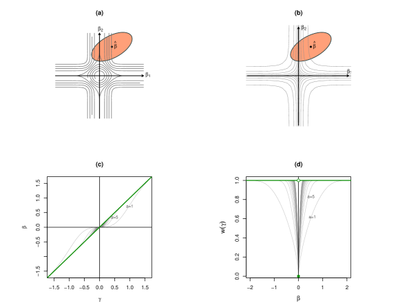
for some $t_{0}\geq 0$. Figure 2(a) presents a graphical illustration of the optimization problem (2.4) in the two-dimensional case. The objective function in (2.4) is an ellipsoid centered at MLE $\widehat{\mbox{\boldmath$\beta$}}$. The feasible set for the constraint $w(\beta_{1})+w(\beta_{2})\leq t_{0}$ contains both sharpened diamonds for large $t_{0}$ and discs for small $t_{0}$ as shown in the contour plots of Figure 2(a). By the Taylor expansion, $w(\beta)=a\beta^{2}+O(\beta^{6})$ for $\beta\rightarrow 0$. Thus, it is not surprising that $w(\beta)$ behaves similarly to the ridge $\ell_{2}$ penalty around 0. This implies that sparsity may not be enforced. We shall address this issue in the next section. Hereafter, we consider $w(\beta)$ to be the hyperbolic tangent penalty, unless otherwise explicitly stated.

Figure 2: Illustration of the reparameterization step: (a) the contour plot for the optimization problem in the two-dimensional scenario before reparameterization; (b) the contour plot after reparameterization; (c) $\beta=\gamma w(\gamma)$ vs. $\gamma$; and (d) $w(\gamma)$ as a penalty function for $\beta$. Different $a$ values in {1, 5, 10, 15, …, 100} are used .

2.2 Reparameterization

To enforce sparsity, we consider a reparameterization procedure originally motivated from the nonnegative garrotte (NG) of Breiman (1995). NG can be viewed as a sign-constrained regularization that is based on the decomposition $\beta=\mbox{sgn}(\beta)|\beta|$. Supposing that the sign of each $\beta_{j}$ can be correctly specified by the MLE $\widehat{\mbox{\boldmath$\beta$}}$, it remains to estimate $|\mbox{\boldmath$\beta$}_{j}|$. Reparameterizing $\mbox{\boldmath$\beta$}=\mbox{diag}(\widehat{\mbox{\boldmath$\beta$}})\,\mbox{\boldmath$\gamma$}$ for some nonnegative vector $\gamma$ such that $\gamma_{j}=|\beta_{j}|$ leads to the NG formulation

$$\min_{\mbox{\boldmath$\gamma$}}-2L(\mbox{\boldmath$\beta$})\mbox{~{}~{}s.t.~{}}\sum_{j=1}^{p}\gamma_{j}\leq t\mbox{~{}and~{}}\gamma_{j}\geq 0,$$

where $t$ is a tuning parameter. One fundamental problem with sign-constrained regularization is that if any sign is wrongly specified by the initial estimator $\widehat{\mbox{\boldmath$\beta$}}$, which occurs often with real data owing to multicollinearity or other complexities, then it is not possible to make correction.

Our immediate aim is to introduce singularity to the penalty function at 0. For this purpose, we consider the decomposition $\beta=\beta\,I\{\beta\neq 0\}$. Set $\gamma=\beta$ and approximate $I\{\gamma\neq 0\}$ with $w(\gamma)$. Namely,

$$\gamma\,=\,\gamma\,I\{\gamma\neq 0\}~{}\approx~{}\gamma w(\gamma).$$

This motivates the reparameterization $\beta_{j}$ as $\beta_{j}=\gamma_{j}w(\gamma_{j})$ for $j=1,\ldots,p.$ In matrix form, $\mbox{\boldmath$\beta$}=\mathbf{W}\mbox{\boldmath$\gamma$},$ where matrix $\mathbf{W}$ is defined earlier in (2.1). As shown in Figure 2(c), $\beta$ is an strictly increasing function of $\gamma$ and $\beta=\gamma$ except for a small neighborhood of 0, in which a shrinkage on $|\beta|$ is imposed.

To see how the reparameterization helps with enforcing sparsity, consider the resulting optimization problem:

$$\min_{\mbox{\boldmath$\beta$}}~{}~{}-2\cdot L(\mbox{\boldmath$\beta$})+\ln(n)\cdot\sum_{j=1}^{p}w(\gamma_{j}).$$ (2.5)

Compared to (2.3), the only change is that the penalty function $w(\cdot)$ is now applied to the reparameterized $\gamma_{j}$ instead of $\beta_{j}.$ It is worth noting that the penalty function $w(\gamma_{j})$ in (2.5) is an implicit function of $\beta_{j}$. Figure 2(d) plots $w(\gamma)$ as a penalty function of $\beta$ for different values of $a,$ which now shows a similar pattern to the non-convex SCAD or MCP penalty with a cusp at $\beta=0$. It can be easily verified that $w(\gamma)$ remains a unit dent function of $\beta$ that well approximates $I(\beta\neq 0).$

The singularity at 0 can be further confirmed by calculating the derivatives of $w(\gamma)$ at $\beta$. Applying the chain rule gives

$$\frac{d\,w(\gamma)}{d\,\beta}=\frac{d\,w(\gamma)}{d\,\gamma}\cdot\frac{d\,\gamma}{d\,\beta}=\frac{d\,w(\gamma)}{d\,\gamma}\cdot\left(\frac{d\,\beta}{d\,\gamma}\right)^{-1}=\frac{\displaystyle\dot{w}}{\displaystyle w+\gamma\dot{w}},$$ (2.6)

where we denote $w=w(\gamma)$ and $\dot{w}=\dot{w}(\gamma)=2a\gamma(1-w^{2}),$ and it follows $d\,\beta/d\,\gamma=w+\gamma\dot{w}.$ The first derivative in (2.6) is expressed in terms of $\gamma$ via implicit differentiation since the explicit formula of $\gamma$ in terms of $\beta$ is unavailable. The validity of (2.6), however, requires $d\,\beta/d\,\gamma~{}\neq~{}0$, which holds everywhere except at $\beta=0.$ Similar arguments can be used to derive the form of the higher-order derivatives. For example, the second-derivative is given by

$$\frac{\displaystyle d^{2}\,w(\gamma)}{\displaystyle d\,{\beta}^{2}}=\frac{\displaystyle w\,\ddot{w}-2\,\dot{w}^{2}}{\displaystyle(w+\gamma\dot{w})^{3}}$$

with $\ddot{w}=\ddot{w}(\gamma)=2a(1-w^{2})(1-4a\gamma^{2}w),$ which again does not exist at $\beta=0.$ It can be verified that $w(\gamma)$ is a smooth function of $\beta$ except at $\beta=0.$

It is worth mentioning that the property that the reparameterization $\beta=\gamma w(\gamma)$ helps enforce singularity at 0 holds for any smooth function in $\mathcal{D}$. We have utilized the differentiation of the inverse function to achieve this. Accordingly, the derivatives of $w(\gamma)$ as a function of $\beta$ exist everywhere except when $\beta=0$. There should be other ways of introducing singularities for smooth functions.

Figure 2(b) provides a two-dimensional illustration of the constrained optimization version that corresponds to (2.5):

$$\min_{\mbox{\boldmath$\beta$}}~{}~{}(\mbox{\boldmath$\beta$}-\widehat{\mbox{\boldmath$\beta$}})^{T}\left\{-\,\nabla^{2}L(\widehat{\mbox{\boldmath$\beta$}})\right\}(\mbox{\boldmath$\beta$}-\widehat{\mbox{\boldmath$\beta$}})\mbox{~{}~{}subject to~{}~{}}\mbox{tr}(\mathbf{W})\leq t_{0}\mbox{~{}with~{}}\mbox{\boldmath$\beta$}=\mathbf{W}\mbox{\boldmath$\gamma$}.$$

The contour lines of the constraint $w(\gamma_{1})+w(\gamma_{2})\leq t$ (as a function of $\beta_{1}$ and $\beta_{2}$ now) become sharpened diamonds, which serves better for the variable selection purpose.

Besides achieving sparsity, the smooth formulation facilitated by reparameterization allows us to further capitalize on available results in both optimization theory and statistical inference and leads to some important conveniences and advantages. For the computation purpose, we shall estimate $\gamma$ instead by solving (2.1). Compared to (2.5) where the objective function is nonsmooth in $\beta$, we have now switched the decision vector to $\gamma$ instead of $\mbox{\boldmath$\beta$}.$ Solving (2.1) is a smooth optimization problem and many standard algorithms can be applied. Estimation of $\gamma$ is meaningful in its own right. The fact that the correspondence between $\beta$ and $\gamma$ is one-to-one with $\beta_{j}=0$ iff $\gamma_{j}=0$ allows us to derive significance testing results for $\beta$ through $\gamma$, which are free of post-selection inference. The objective function in (2.1) is smooth for estimating $\mbox{\boldmath$\gamma$}.$ Thus standard arguments in M-estimators can be applied for obtaining inference on $\mbox{\boldmath$\gamma$}.$ The detailed procedure will be explained in next section.

3 Asymptotic Properties

In this section, we first study the asymptotic oracle properties of the MIC estimator $\widetilde{\mbox{\boldmath$\beta$}}$, including its $\sqrt{n}$-consistency, selection consistency, and the asymptotic normality of its nonzero components. We then present significance testing on $\beta$ via $\gamma$, which is free of post-selection inference. Once again, we emphasize that all our discusses are restricted to the fixed $p$ scenarios.

3.1 Oracle Properties of the MIC Estimator $\widetilde{\mbox{\boldmath$\beta$}}$

For theoretical investigation, we consider the MIC estimator $\widetilde{\mbox{\boldmath$\beta$}}$ obtained from minimizing the objective function in (2.5)

$$Q_{n}(\mbox{\boldmath$\beta$})=-2\,\frac{L(\mbox{\boldmath$\beta$})}{n}+\frac{\ln(n)}{n}\,\sum_{j=1}^{p}w(\gamma_{j}),$$ (3.1)

where $L(\mbox{\boldmath$\beta$})=\sum_{i=1}^{n}l_{i}(\mbox{\boldmath$\beta$})$ with $l_{i}(\mbox{\boldmath$\beta$})=\log f(\mathbf{X}_{i},Y_{i};\mbox{\boldmath$\beta$})$. We shall denote $a$ as $a_{n}$ so that $\beta_{j}=\gamma_{j}w(\gamma_{j})=\gamma_{j}\tanh(a_{n}\beta_{j}^{2})$ and assume $a_{n}=O(n)$; this rate for $a_{n}$ will be manifested in the derivation.

Denote the true parameter as $\mbox{\boldmath$\beta$}_{0}=({\mbox{\boldmath$\beta$}}_{0(1)}^{T},{\mbox{\boldmath$\beta$}}_{0(0)}^{T})^{T},$ where ${\mbox{\boldmath$\beta$}}_{0(1)}\in\mathbb{R}^{q}$ consists of all $q$ nonzero components and ${\mbox{\boldmath$\beta$}}_{0(0)}=\mathbf{0}$ consists of all the $(p-q)$ zero components. As generic notation, we use $\widetilde{\mbox{\boldmath$\beta$}}$ and $\widehat{\mbox{\boldmath$\beta$}}$ to denote the MIC and MLE estimators, respectively. Let $\mathbf{I}=\mathbf{I}(\mbox{\boldmath$\beta$}_{0})$ be the expected Fisher information matrix for the whole model and let $\mathbf{I}_{1}$ be the Fisher information corresponding to the reduced true model setting $\mbox{\boldmath$\beta$}_{0(0)}=\mathbf{0}.$ It is well known that $\mathbf{I}_{1}$ is the $q$-th principal submatrix of $\mathbf{I}.$ The following theorem shows that, under regularity conditions, there exists a local minimizer $\widetilde{\mbox{\boldmath$\beta$}}$ of $Q_{n}(\mbox{\boldmath$\beta$})$ that is $\sqrt{n}$-consistent and this $\sqrt{n}$-consistent $\widetilde{\mbox{\boldmath$\beta$}}$ enjoys the ‘oracle’ property.

Theorem 3.1.

Let $\{(\mathbf{X}_{i},Y_{i}):i=1,\ldots,n\}$ be $n$ i.i.d. copies from a density $f(\mathbf{X},Y;\mbox{\boldmath$\beta$}_{0}).$ Under the regularity conditions (A)–(C) in Fan and Li (2001), we have

1. ($\sqrt{n}$-Consistency)   there exists a local minimizer $\widetilde{\mbox{\boldmath$\beta$}}$ of $Q_{n}(\mbox{\boldmath$\beta$})$ that is $\sqrt{n}$-consistent for $\mbox{\boldmath$\beta$}_{0}$ in the sense that $\parallel\widetilde{\mbox{\boldmath$\beta$}}-\mbox{\boldmath$\beta$}_{0}\parallel=O_{p}(n^{-1/2}).$

2. (Sparsity and Asymptotic Normality)   Partition $\widetilde{\mbox{\boldmath$\beta$}}$ in (i) as $(\widetilde{\mbox{\boldmath$\beta$}}_{(1)}^{T},\widetilde{\mbox{\boldmath$\beta$}}_{(0)}^{T})^{T}$ in a similar manner to $\mbox{\boldmath$\beta$}_{0}$. With probability tending to 1 as $n\rightarrow\infty$, $\widetilde{\mbox{\boldmath$\beta$}}$ must satisfy that

   $$\widetilde{\mbox{\boldmath$\beta$}}_{(0)}=\mathbf{0}$$

   and

   $$\sqrt{n}(\widetilde{\mbox{\boldmath$\beta$}}_{(1)}-\mbox{\boldmath$\beta$}_{0(1)})\,\rightarrow\,N\left(\mathbf{0},\,\mathbf{I}_{1}^{-1}\right).$$

The results in Theorem 3.1 are analogous to Theorems 1 & 2 in Fan and Li (2001). It establishes that $\widetilde{\mbox{\boldmath$\beta$}}_{(0)}$ is selection consistent and $\widetilde{\mbox{\boldmath$\beta$}}_{(1)}$ is a best asymptotic normal (BAN; see, e.g., Serfling, 1980) estimator of $\mbox{\boldmath$\beta$}_{0(1)}.$ We defer its proof to the Appendix. The standard errors (SE) for nonzero components in $\widetilde{\mbox{\boldmath$\beta$}}$ can be conveniently computed by replacing $\mathbf{I}_{1}$ in Theorem 3.1(ii) with the observed Fisher information matrix (Efron and Hinkley, 1978) and plugging in $\widetilde{\mbox{\boldmath$\beta$}}$. Since $\widetilde{\mbox{\boldmath$\beta$}}$ is essentially an M-estimator, alternative sandwich SE formulas (Stefanski and Boos, 2002) are available, for which we shall not pursue further. However, as post-selection inferences, all these SE formulas are only available for nonzero components in $\widetilde{\mbox{\boldmath$\beta$}}$ and hence caution should be exercised.

Table 1: Simulation results on MIC (with $\lambda_{0}=\ln(n)$ and $a=10$) in comparison with other methods. Reported quantities include the averaged model errors (ME), the averaged model size (Size), the average number of false positive variables (FP), the average number of false negative variables (FN), the proportion of correct selections (C), all based on 500 realizations.

(a) Model A – Linear Regression
	$n=100$					$n=200$
Method	ME	Size	FP	FN	C	ME	Size	FP	FN	C
MIC	0.054	3.47	0.47	0.00	0.640	0.021	3.25	0.25	0.00	0.790
Oracle	0.034	3.00	0.00	0.00	1.000	0.015	3.00	0.00	0.00	1.000
BIC	0.055	3.35	0.35	0.00	0.710	0.022	3.19	0.19	0.00	0.834
LASSO	0.085	6.09	3.09	0.00	0.092	0.039	6.23	3.23	0.00	0.102
SCAD	0.045	3.58	0.58	0.00	0.752	0.022	3.71	0.71	0.00	0.752
MCP	0.047	3.57	0.57	0.00	0.750	0.020	3.41	0.41	0.00	0.814

(b) Model B – Logistic Regression
	$n=100$					$n=200$
Method	ME	Size	FP	FN	C	ME	Size	FP	FN	C
MIC	0.017	3.74	1.03	0.29	0.354	0.005	3.42	0.49	0.07	0.624
Oracle	0.005	3.00	0.00	0.00	1.000	0.002	3.00	0.00	0.00	1.000
BIC	0.015	3.40	0.67	0.27	0.514	0.005	3.21	0.28	0.06	0.766
LASSO	0.023	6.54	3.79	0.25	0.012	0.012	7.32	4.37	0.05	0.018
SCAD	0.019	3.69	1.09	0.41	0.206	0.012	3.92	1.11	0.19	0.278
MCP	0.019	3.12	0.65	0.53	0.236	0.011	3.39	0.64	0.24	0.420

(c) Model C – Log-Linear Regression
	$n=100$					$n=200$
Method	ME	Size	FP	FN	C	ME	Size	FP	FN	C
MIC	12.310	3.34	0.35	0.00	0.712	4.367	3.23	0.23	0.00	0.828
Oracle	9.289	3.00	0.00	0.00	1.000	3.555	3.00	0.00	0.00	1.000
BIC	25.884	3.39	0.39	0.00	0.714	4.897	3.23	0.23	0.00	0.826
LASSO	600.821	1.55	0.37	1.81	0.184	348.182	1.46	0.18	1.72	0.282
SCAD	40.753	4.08	1.08	0.00	0.336	12.843	3.64	0.64	0.00	0.528

3.2 Inference on $\beta$ via $\gamma$

MIC avoids the two-step estimation process in the best subset selection and regularization by completing both variable selection and parameter estimation in one single optimization step. This brings about a unique opportunity to address the fundamental post-selection inference problem.

Inference on zero components in $\beta$ is unavailable in MIC. This is because asymptotic normality of M-estimators often involves a condition that the expected objective function $E\{Q_{n}(\mbox{\boldmath$\beta$})\}$ admits a second-order Taylor expansion at $\mbox{\boldmath$\beta$}_{0}$ whereas sparsity requires singularity of the penalty function $w(\gamma)$ as a function of $\beta$ at $\beta=0.$ However, the reparameterisation helps us to circumvent this non-smoothness issue. The transformation $\beta=\gamma w(\gamma)$ is a bijection and $\beta=0$ iff $\gamma=0.$ Therefore, testing $H_{0}:~{}\beta_{j}=0$ is equivalent to testing $H_{0}:\gamma_{j}=0.$ As the objective function of $\gamma$, $Q_{n}(\mbox{\boldmath$\gamma$})$ in (3.1) is smooth in $\mbox{\boldmath$\gamma$}.$ Therefore, the statistical properties of $\widetilde{\mbox{\boldmath$\gamma$}}$ are readily available following standard M-estimation arguments, as given in the theorem below.

Theorem 3.2.

Let $\mbox{\boldmath$\gamma$}_{0}$ be the reparameterized parameter vector associated with $\mbox{\boldmath$\beta$}_{0}$ such that $\beta_{0j}=\gamma_{0j}w(\gamma_{0j}).$ It follows that $\parallel\mbox{\boldmath$\gamma$}_{0}-\mbox{\boldmath$\beta$}_{0}\parallel_{2}=O\{\exp(-2a_{n}\min_{1\leq j\leq q}\gamma^{2}_{0j})\}.$ Under the regularity conditions (A)–(C) in Fan and Li (2001), we have

$$\sqrt{n}\left[\mathbf{D}(\mbox{\boldmath$\gamma$}_{0})(\widetilde{\mbox{\boldmath$\gamma$}}-\mbox{\boldmath$\gamma$}_{0})+\mathbf{b}_{n}\right]~{}\stackrel{{\scriptstyle d}}{{\longrightarrow}}~{}N\left\{\mathbf{0},\,\mathbf{I}^{-1}(\mbox{\boldmath$\beta$}_{0})\right\}.$$ (3.2)

where

$$\mathbf{D}(\mbox{\boldmath$\gamma$}_{0})=\left.\mbox{diag}(w_{j}+\gamma_{j}\dot{w}_{j})\right|_{\mbox{\boldmath$\gamma$}=\mbox{\boldmath$\gamma$}_{0}}=\mbox{diag}\left(D_{jj}\right)$$ (3.3)

and the asymptotic bias

$$\mathbf{b}_{n}=\left\{-\nabla^{2}L(\mbox{\boldmath$\beta$}_{0})\right\}^{-1}\,\frac{\ln(n)}{2}\left(\frac{\dot{w}_{j}}{w_{j}+\tilde{\gamma}_{j}\dot{w}_{j}}\right)_{j=1}^{p}\,=\,\left(b_{nj}\right)_{j=1}^{p}$$ (3.4)

satisfy (i) $\lim_{n\rightarrow\infty}D_{jj}=I\{\beta_{0j}\neq 0\}$ and (ii) $\mathbf{b}_{n}=o_{p}(1).$

The proof of Theorem 3.2 is given in the Appendix. One practical implication of Theorem 3.2 is that both $\mathbf{D}(\mbox{\boldmath$\gamma$}_{0})$ and $\mathbf{b}_{n}$ may be ignored in computing the standard errors of $\widetilde{\mbox{\boldmath$\gamma$}}.$ Furthermore, since $\parallel\widetilde{\mbox{\boldmath$\gamma$}}-\mbox{\boldmath$\beta$}_{0}\parallel\,\leq\,\parallel\widetilde{\mbox{\boldmath$\gamma$}}-\mbox{\boldmath$\gamma$}_{0}\parallel+\parallel\mbox{\boldmath$\gamma$}_{0}-\mbox{\boldmath$\beta$}_{0}\parallel=o_{p}(1),$ $\widetilde{\mbox{\boldmath$\gamma$}}$ is a consistent estimator of $\mbox{\boldmath$\beta$}_{0}$ and can be used to replace $\mbox{\boldmath$\beta$}_{0}$ in estimating the Fisher information matrix. Thus, an asymptotic $(1-\alpha)\times 100\%$ confidence interval for $\gamma_{0j}$ can be simply given by

$$\tilde{\gamma}_{j}\,\pm\,z_{1-\alpha/2}\,\sqrt{\left(\mathbf{I}_{n}^{-1}(\widetilde{\mbox{\boldmath$\gamma$}})/n\right)_{jj}},$$ (3.5)

where $\mathbf{I}_{n}$ denotes the observed Fisher information matrix and $z_{1-\alpha/2}$ is the $(1-\alpha/2)$-th percentile of $N(0,1).$ Significance testing on $\gamma_{0j}$ can be done accordingly. There are alternative ways to derive the asymptotic variance of $\widetilde{\mbox{\boldmath$\beta$}}$. We numerically experimented a couple of other sandwich estimators and found that the simple formula in (3.5) performs very well empirically.

4 Numerical Results

In this section, we present simulation experiments and real data examples to illustrate MIC in comparison with other methods.

4.1 Computational Issues

MIC solves for $\widetilde{\mbox{\boldmath$\gamma$}}$ by optimizing (2.1). Considering its nonconvex nature, a global optimization method is desirable. Mullen (2014) provides a comprehensive comparison of many global optimization algorithms currently available in R (R Core Team, 2016). According to her recommendations, we have chosen the GenSA package (Xiang et al., 2013) that implements the generalized simulation annealing of Tsallis and Stariolo (1996), because of its superior performance in both identification of the true optimal point and computing speed. With estimated $\widetilde{\mbox{\boldmath$\gamma$}}$, the MIC estimator $\widetilde{\mbox{\boldmath$\beta$}}$ of $\beta$ can be obtained immediately via the transformation $\widetilde{\mbox{\boldmath$\beta$}}=\widetilde{\mathbf{W}}\widetilde{\mbox{\boldmath$\gamma$}}$, where $\widetilde{\mathbf{W}}=\mbox{diag}(\tilde{w}_{j})$ with $\tilde{w}_{j}=w(\tilde{\gamma}_{j}).$ Because of the shrinkage effect of the reparameterization around 0, estimates $\tilde{\gamma}_{j}$ that are close to 0 would yield very small values of $\tilde{\beta}_{j}$, which can be virtually taken as 0.

Implementation of MIC involves of the choice of $a_{n}$. In theory, the asymptotic results in Section 3 entail that $a_{n}=O(n).$ In order to apply the arguments of Fan and Li (2001), this $O(n)$ rate seems unique. See the proofs of Theorem 3.1 in the appendix. On the other hand, if one is willing to adjust the choice of $\lambda_{0}$, recall that the selection consistency of BIC holds for a wide range of $\lambda$ values, then the choice of $a_{n}$ can be more flexible. However, the conventional choice of $\lambda_{0}=\ln(n)$ is optimal in the Bayesian sense (Schwarz, 1978). Thus it is advisable to keep it as is. In practice, the empirical performance of MIC stays rather stable with respect to the choice of $a_{n},$ as demonstrated in Su (2015) for linear regression. The role of $a$ is quite different from the tuning parameter $\lambda$ in regularization that controls the penalty for complexity or the range of certain constraints. When $\lambda$ varies, the parameter estimates would change dramatically, which necessitates selection of $\lambda.$ In MIC, $a_{n}$ is a shape or scale parameter in the unit dent function that modifies the sharpness of its approximation to the indicator function. The role of $a_{n}$ is largely similar to that of the parameter $a$ in SCAD (Fan and Li, 2001), where $a$ is fixed as $a=3.7.$ In general, a larger $a_{n}$ value enforces a better approximation of the indicator function with the hyperbolic tangent function. On the other hand, a smaller $a_{n}$ is appealing for optimization purposes, by introducing more smoothness. Based on our numerical experiences, applying a $a$ value smaller than 1 leads to less stable and reduced performance. The performance of MIC stabilizes substantially when $a_{n}$ gets large, especially when it is 10 or above. On this basis, we recommend choosing $a_{n}$ at a value in [10, 50] for standardized data. Avoiding tuning $a_{n}$ makes MIC computationally advantageous.

Four known methods are included for comparison with MIC: the best subset selection (BSS) with BIC, LASSO, SCAD, and MCP. The oracle estimate is also added as a benchmark. All the computations are done in R (R Development Core Team, 2015). Specifically, we have used the R package bestglm for BSS, lars and glmnet for LASSO, and ncvreg and SIS for SCAD and MCP. The default settings are used in these implementations, presuming that the default setting is the most recommendable.

Table 2: Simulation results on standard errors of nonzero $\widehat{\mbox{\boldmath$\beta$}}$ with $n=200$ over 500 simulation runs. Reported quantities are MAD of the parameter estimates, Median of the standard errors, and MAD of the standard errors.

(a) Model A – Gaussian Linear Regression
	oracle			MIC			Best Subset
Parameter	MAD	Median SE	MAD SE	MAD	Median SE	MAD SE	MAD	Median SE	MAD SE
$\beta_{1}$	0.083	0.082	0.006	0.083	0.082	0.006	0.084	0.082	0.004
$\beta_{2}$	0.084	0.082	0.006	0.087	0.082	0.006	0.085	0.082	0.004
$\beta_{5}$	0.072	0.072	0.005	0.073	0.072	0.005	0.075	0.072	0.004

(b) Model B – Logistic Regression
	oracle			MIC			Best Subset
Parameter	MAD	Median SE	MAD SE	MAD	Median SE	MAD SE	MAD	Median SE	MAD SE
$\beta_{1}$	0.528	0.475	0.086	0.529	0.492	0.094	0.545	0.488	0.090
$\beta_{2}$	0.399	0.389	0.048	0.448	0.407	0.064	0.435	0.400	0.057
$\beta_{5}$	0.380	0.356	0.059	0.405	0.367	0.061	0.402	0.362	0.061

(c) Model C – Loglinear Regression
	oracle			MIC			Best Subset
Parameter	MAD	Median SE	MAD SE	MAD	Median SE	MAD SE	MAD	Median SE	MAD SE
$\beta_{1}$	0.037	0.036	0.007	0.037	0.036	0.007	0.038	0.036	0.007
$\beta_{2}$	0.039	0.039	0.007	0.040	0.039	0.007	0.041	0.039	0.007
$\beta_{5}$	0.032	0.032	0.006	0.033	0.033	0.006	0.033	0.033	0.006

Table 3: Hypothesis testing on $\mbox{\boldmath$\gamma$}_{0}$ in MIC. Empirical size and empirical power are obtained at the significance level $\alpha=0.05$ based on 1,000 simulation runs.

		Empirical Size									Empirical Power
Model	$n$	$\gamma_{3}$	$\gamma_{4}$	$\gamma_{6}$	$\gamma_{7}$	$\gamma_{8}$	$\gamma_{9}$	$\gamma_{10}$	$\gamma_{11}$	$\gamma_{12}$	$\gamma_{1}$	$\gamma_{2}$	$\gamma_{5}$
A	100	0.054	0.059	0.061	0.060	0.055	0.056	0.054	0.051	0.044	1.000	1.000	1.000
	200	0.049	0.040	0.047	0.040	0.034	0.024	0.039	0.036	0.031	1.000	1.000	1.000
B	100	0.054	0.059	0.061	0.060	0.055	0.056	0.054	0.051	0.044	1.000	1.000	1.000
	200	0.049	0.040	0.047	0.040	0.034	0.024	0.039	0.036	0.031	1.000	1.000	1.000
C	100	0.042	0.048	0.047	0.034	0.030	0.034	0.036	0.044	0.041	1.000	1.000	1.000
	200	0.022	0.025	0.025	0.042	0.024	0.029	0.023	0.021	0.024	1.000	1.000	1.000

4.2 Simulated Experiments

We generate data sets from the following three GLM models by using the same simulation settings as those of Zou and Li (2008). Specifically, the following three models are used:

$$\left\{\begin{array}[]{ll}\mbox{Model A:~{}}&y|\mathbf{x}~{}\sim~{}N\{\mu(\mathbf{x}),1\}\mbox{~{}~{}with~{}}\mu(\mathbf{x})=\mathbf{x}^{T}\mbox{\boldmath$\beta$},\\ \mbox{Model B:~{}}&y|\mathbf{x}~{}\sim~{}\mbox{Bernoulli}\{\mu(\mathbf{x})\}\mbox{~{}~{}with~{}}\mu(\mathbf{x})=\mbox{expit}(\mathbf{x}^{T}\mbox{\boldmath$\beta$}),\\ \mbox{Model C:~{}}&y|\mathbf{x}~{}\sim~{}\mbox{Poisson}\left\{\mu(\mathbf{x})\right\}\mbox{~{}~{}with~{}}\mu(\mathbf{x})=\exp(\mathbf{x}^{T}\mbox{\boldmath$\beta$}),\end{array}\right.$$ (4.1)

where $\mbox{\boldmath$\beta$}=(3,1.5,0,0,2,0,0,0,0,0,0,0)^{T}$ in Models A and B, and $(1.2,.6,0,0,.8,0,0,0,0,0,0,0)^{T}$ in Model C. Each data set involves $p=12$ predictors that follow a multivariate normal distribution $N(\mathbf{0},\,\mbox{\boldmath$\Sigma$})$ with $\mbox{\boldmath$\Sigma$}=(\sigma_{jj^{\prime}})$ and $\sigma_{jj^{\prime}}=0.5^{|j-j^{\prime}|}$ for $j,j^{\prime}=1,\ldots,p.$ In Model B, six binary predictors are created by setting $x_{2j-1}:=I(x_{2j-1}<0)$ for $j=1,\ldots,6.$ Thus, there are six continuous and six binary predictors in Model B. Each simulation includes two different sample sizes $n=100$ and $n=200$, and 500 realizations are generated from each model.

To apply the MIC method, we fix $\lambda_{0}=\ln(n)$ and $a_{n}=10.$ Five performance measures are used for making comparisons. The first one is the empirical model error (ME), defined as $\mbox{ME}=\sum_{i=1}^{n}(\mu_{i}-\hat{\mu}_{i})^{2}/n$, where $\mu_{i}$ is given in (4.1) and $\hat{\mu}_{i}$ is obtained by plugging in the estimate of $\beta$. We compute ME based on an independent test sample of size $n=500$ and then report the averaged ME over $500$ realizations. The other measures are the average model size (Size; defined as the number of nonzero parameter estimates), the average number of false positives (FP; defined as the number of nonzero estimates for zero parameters), the average number of false negatives (FN; defined as the number of zero estimates for nonzero parameters), and the proportion of correct selections (C).

Table 1 indicates that MIC performs similarly to BSS with BIC across all three models. In addition, all performance measures of MIC improve as the sample size increases. By comparing MIC against the other regularization methods, we find that MIC outperforms them in general, except for the Gaussian linear regression case where its performance is only comparable. We think this is mainly because the objective function of MIC involves the Gaussian profile likelihood $n\ln\parallel\mathbf{y}-\mathbf{X}\mbox{\boldmath$\beta$}\parallel^{2}$, which is nonconvex, while regularization methods can work with the convex least squares problem $\parallel\mathbf{y}-\mathbf{X}\mbox{\boldmath$\beta$}\parallel^{2}$ directly. Nevertheless, they all have to deal with the same log-likelihood function in Model B and C. Note that no implementation of MCP is available for the log-linear regression, hence it is not presented for Model C. In sum, MIC not only enjoys computational efficiency, but also demonstrates good finite sample performance.

We next evaluates the standard error formula for nonzero parameter estimates. Table 2 presents the median absolute deviation (MAD) value of $\widetilde{\mbox{\boldmath$\beta$}}_{(1)}$ out of 500 runs, which provides a more robust estimates of its standard deviation. This MAD value matches reasonably well with the median of standard errors of $\widetilde{\mbox{\boldmath$\beta$}}_{(1)}$. Also presented is the MAD of standard errors.

Table 3 presents the empirical size and power results in testing $H_{0}:~{}\gamma_{j}=0$ at the significance level $\alpha=0.05$ over 1,000 simulation runs. It can be seen that the proposed testing procedure has empirical sizes close to the nominal level $0.05$ while showing excellent empirical power. This result pertains closely to the super-efficiency phenomenon (see, e.g., Chapter 8 of van der Vaart, 1998). Although super-efficiency could occur on at most a Lebesgue null set, it does seem to have an impact practically.

Table 4: Illustration of MIC with real data examples.

(a) Linear Regression with Diabetes Data
	Full Model		Best Subset		MIC
	$\hat{\beta}_{j}$	SE	$\hat{\beta}_{j}$	SE	$\hat{\gamma}_{j}$	SE	P-Value	$\hat{\beta}_{j}$	SE	LASSO	SCAD	MCP
age	$-0.006$	0.037			0.000	0.036	1.000
sex	$-0.148$	0.038	$-0.146$	0.037	$-0.315$	0.037	0.000	$-0.137$	0.037	$-0.122$	$-0.149$	$-0.143$
bmi	0.321	0.041	0.323	0.040	0.406	0.041	0.000	0.325	0.040	0.323	0.321	0.328
map	0.200	0.040	0.202	0.039	0.344	0.040	0.000	0.196	0.039	0.184	0.199	0.197
tc	$-0.489$	0.257			0.000	0.257	1.000			$-0.064$	$-0.381$
ldl	0.294	0.209			0.000	0.209	1.000				0.216	$-0.067$
hdl	0.062	0.131	$-0.179$	0.041	$-0.332$	0.131	0.011	$-0.171$	0.041	$-0.138$		$-0.179$
tch	0.109	0.100			0.000	0.099	1.000				0.080
ltg	0.464	0.106	0.293	0.041	0.390	0.106	0.000	0.294	0.041	0.318	0.426	0.300
glu	0.042	0.041			0.000	0.040	1.000			0.034	0.041	0.030
BIC	998.00		975.82		975.82					982.62	986.07	1001.64

(b) Logistic Regression with Heart Data
	Full Model		Best Subset		MIC
	$\hat{\beta}_{j}$	SE	$\hat{\beta}_{j}$	SE	$\hat{\gamma}_{j}$	SE	P-Value	$\hat{\beta}_{j}$	SE	LASSO	SCAD	MCP
intercept	$-0.845$	0.120	$-0.847$	0.120	$-0.842$	0.122	0.000	$-0.842$	0.119	$-0.787$	$-0.846$	$-0.844$
sbp	0.118	0.115			0.000	0.116	1.000			0.041		0.062
tobacco	0.365	0.120	0.371	0.117	0.418	0.123	0.001	0.349	0.116	0.299	0.371	0.369
ldl	0.383	0.119	0.347	0.112	0.407	0.120	0.001	0.326	0.111	0.271	0.350	0.368
famhist	0.463	0.111	0.456	0.110	0.476	0.112	0.000	0.446	0.110	0.371	0.456	0.460
obesity	$-0.146$	0.123			0.000	0.121	1.000			$-0.011$	$-0.086$
alcohol	0.015	0.109			0.000	0.101	1.000
age	0.621	0.149	0.643	0.142	0.656	0.152	0.000	0.656	0.142	0.544	0.645	0.632
BIC	532.26		516.12		516.12					526.14	521.11	521.44

(c) Log-Linear Regression with Fish Data
	Full Model		Best Subset		MIC
	$\hat{\beta}_{j}$	SE	$\hat{\beta}_{j}$	SE	$\hat{\gamma}_{j}$	SE	P-Value	$\hat{\beta}_{j}$	SE	LASSO	SCAD
intercept	$-0.360$	0.090	$-0.313$	0.073	$-0.395$	0.091	0.000	$-0.304$	0.073	0.357	$-1.233$
nofish	$-0.033$	0.059			0.000	0.061	1.000
livebait	0.129	0.090			0.000	0.081	1.000				0.426
camper	$-0.010$	0.051			0.000	0.053	1.000
persons	0.047	0.057			0.000	0.059	1.000
child	$-0.653$	0.103	$-0.643$	0.098	$-0.639$	0.106	0.000	$-0.638$	0.098		$-0.778$
xb	1.447	0.064	1.467	0.034	1.464	0.067	0.000	1.464	0.034	0.331	1.012
zg	0.659	0.136	0.604	0.067	0.606	0.142	0.000	0.604	0.067		0.283
xb:zg	$-0.034$	0.059			0.000	0.061	1.000			0.176	$-0.001$
BIC	636.551		613.91		613.91					850.54	621.08

4.3 Real Data Examples

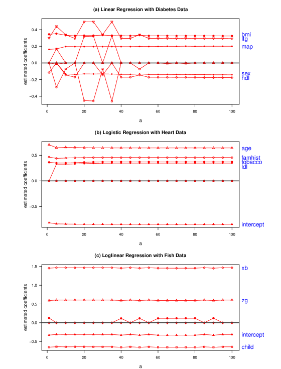
We consider the diabetes data (Efron et al., 2004), the heart data (Hastie, Tisshirani, and Friedman, 2009), and the fish count data (available at http://www.ats.ucla.edu/stat/data/fish.csv) to illustrate linear regression, logistic regression, and log-linear regression models, respectively.

Table 4 shows that MIC (with $\lambda_{0}=\ln(n)$ and $a=10$) provides the similar selection as the best subset selection across all three examples. In addition, the resulting MIC estimates and their standard errors are quite close to these of the BIC model. This finding indicates that MIC approximates the best subset selection method well. This, together with MIC’s computational efficacy, allows us to employ MIC on data with large numbers of covariates, even when BSS becomes infeasible. In the diabetes data, it is particularly interesting to note that the sign of the parameter estimate on hdl is positive under the full model fitting, but becomes negative in MIC and several other methods. This sign change could be problematic for sign-constrained methods such as NG (Breiman, 1995), but it comes out naturally in MIC.

To illustrate the stability of MIC with respect to the value of $a$, we obtain the MIC estimates for $a\in\{1,5,10,15,\ldots,100\}$ and then plot them in Figure 3. While there are some reasonable minor variations mainly owning to the non-convex optimization nature, almost all the estimated coefficients are quite steady in all three examples, showing that the MIC estimation is generally robust to the choice of $a.$

Figure 3: Illustrating the robustness of MIC with respect to the choice of $a$ in three real examples. The values of $a$ considered are $\{1,5,10,15,\ldots,100\}$.

5 Discussion

MIC is the first method that does sparse estimation by explicitly approximating BIC. BIC is optimal in two aspects: it approximates the posterior distribution of candidate models besides being selection-consistent. This is why BIC has been used as an ultimate yardstick in various variable selection and regularization methods. MIC extends the best subset selection to scenario with large $p$ by optimizing an approximated BIC. Formulated as a smooth optimization problem, MIC is computationally advantageous to the discrete-natured best subset selection and enjoys the additional benefit in avoiding the post-selection inference. Moreover, the search space in MIC remains to be the entire parameter space. This explains why we expect MIC to outperform many regularization methods that have a much reduced search space for minimum BIC. By borrowing the knowledge of the fixed penalty parameter for model complexity in BIC, MIC circumvents the tuning parameter selection problem and hence is also computationally advantageous to regularization methods.

Although the hyperbolic tangent function has been used to approximate the cardinality in MIC, it can be replaced by other unit dent functions. Since one focus of this paper is on the variable selection consistency, we have adopted BIC by taking $\lambda_{0}=\ln(n)$. In contrast, if the aim is on the model selection efficiency or predictive accuracy, then we can adopt AIC by setting $\lambda_{0}=2$. It can be shown that the resulting MIC is selection-efficient by applying similar techniques to those used in Zhang, Li, and Tsai (2010). In sum, we can obtain variants of MIC by changing its penalty function $w$ and penalty parameter $\lambda_{0}$ to meet practical needs.

To broaden the usefulness of MIC, we conclude this article by discussing three possible avenues for future research. First, generalize MIC by accommodating the grouped or structured sparsity (see, e.g., Huang and Zhang, 2010). Secondly, extend MIC to other complex model or dependence structures, such as finite mixture models, longitudinal data, and structural equation modelings (SEM). Similar ideas may be applied to approximate the effective degrees of freedom as well. In these settings, MIC can be particularly useful because the log-likelihood function is not concave and having convex penalties does not help anything with the optimization problem. Thirdly, develop the MIC method for data with diverging $p\rightarrow\infty$ yet $p/n\rightarrow 0$ (Fan and Peng, 2004) or ultra-high dimensions with $p\gg n$ (Fan and Lv, 2008) by approximating the extended or generalized BIC as pioneered by Chen and Chen (2008).

APPENDIX: PROOFS

Appendix A Proof of Theorem 1

We first establish (i) by checking conditions in Theorem 1 of Fan and Li (2001). Note that the quantity $p_{\lambda_{n}}(|\beta_{j}|)$ corresponds to

$$p_{\lambda_{n}}(|\beta_{j}|)=\frac{\ln(n)}{2n}\cdot w(\gamma_{j}).$$

in MIC. Some quantities involved in the reparameterization $\beta=\gamma w(\gamma)$ are summarized below:

$$\left\{\begin{array}[]{lclcl}\dot{w}&=&dw(\gamma)/d\gamma&=&2a_{n}\gamma(1-w^{2})\\ \ddot{w}&=&d^{2}w(\gamma)/d\gamma^{2}&=&2a_{n}(1-w^{2})(1-4a_{n}\gamma_{0j}^{2}w)\\ w&=&\tanh(a_{n}\gamma^{2})&=&\left(e^{a_{n}\gamma^{2}}-e^{-a_{n}\gamma^{2}}\right)/\left(e^{a_{n}\gamma^{2}}+e^{-a_{n}\gamma^{2}}\right)\\ 1-w^{2}&=&\mbox{sech}(a_{n}\gamma^{2})&=&2/\left(e^{a_{n}\gamma^{2}}+e^{-a_{n}\gamma^{2}}\right)\\ \end{array}\right.$$

Since $a_{n}=O(n)$, $\gamma\rightarrow\beta$ and $w(\gamma)\rightarrow 1$ for $\beta\neq 0$. It follows that, for $\beta\neq 0$,

$$\dot{p}_{\lambda_{n}}(|\beta|) = \frac{dp_{\lambda_{n}}(|\beta|)}{d\,\beta}\,=\,\frac{\ln(n)}{2n}\,\frac{\dot{w}}{w+\gamma\dot{w}}$$

$$= \frac{\ln(n)}{n}\,\frac{a_{n}\gamma(1-w^{2})}{w+2a_{n}\gamma^{2}(1-w^{2})}$$

$$= \frac{\ln(n)}{n}\,\frac{2a_{n}\gamma}{e^{a_{n}\gamma^{2}}+e^{-a_{n}\gamma^{2}}+4a_{n}\gamma^{2}}$$

$$= \frac{\ln(n)}{n}\,O\left\{a_{n}e^{-a_{n}\gamma^{2}}\right\}$$

$$= o(1/\sqrt{n}).$$

Hence, $\max_{j}\left\{\dot{p}_{\lambda_{n}}(|\beta_{0j}|):~{}\beta_{0j}\neq 0\right\}=o(1/\sqrt{n}).$ Similarly, it can be shown that, for $\beta\neq 0$,

$$\ddot{p}_{\lambda_{n}}(|\beta|)=\frac{d^{2}p_{\lambda_{n}}(|\beta|)}{d\,\beta^{2}}=\frac{\ln(n)}{2n}\,\frac{w\ddot{w}-2\dot{w}^{2}}{(w+\gamma\,\dot{w})^{3}}~{}\stackrel{{\scriptstyle p}}{{\longrightarrow}}~{}0.$$

and so is $\max_{j}\left\{\ddot{p}_{\lambda_{n}}(|\beta_{0j}|):~{}\beta_{0j}\neq 0\right\}$.

Therefore, there exists a local minimizer $\widetilde{\mbox{\boldmath$\beta$}}$ of $Q_{n}(\mbox{\boldmath$\beta$})$ such that $\parallel\widetilde{\mbox{\boldmath$\beta$}}-\mbox{\boldmath$\beta$}_{0}\parallel=O_{p}(1/\sqrt{n})$ by Theorem 1 of Fan and Li (2001). $\square$

To establish sparsity of $\widetilde{\mbox{\boldmath$\beta$}}_{(0)}$ in (ii), it suffices to show that, for any $\sqrt{n}$-consistent $\mbox{\boldmath$\beta$}=(\mbox{\boldmath$\beta$}_{(1)}^{T},\mbox{\boldmath$\beta$}_{(0)}^{T})^{T}$ such that $\parallel\mbox{\boldmath$\beta$}_{(1)}-\mbox{\boldmath$\beta$}_{0(1)}\parallel=O_{p}(1/\sqrt{n})$ and $\parallel\mbox{\boldmath$\beta$}_{(0)}\parallel=O_{p}(1/\sqrt{n}),$ we have

$$\frac{\partial Q_{n}(\mbox{\boldmath$\beta$})}{\partial\beta_{j}}=\begin{cases}>0&\mbox{~{}if~{}}\beta_{j}>0\\ <0&\mbox{~{}if~{}}\beta_{j}<0\end{cases}$$ (A.1)

for any component $\beta_{j}$ of $\mbox{\boldmath$\beta$}_{(0)}$ with probability tending to 1 as $n\rightarrow\infty.$

Consider

$$\frac{\partial Q_{n}(\mbox{\boldmath$\beta$})}{\partial\beta_{j}}~{}=~{}-\,\frac{2}{n}\,\frac{\partial l(\mbox{\boldmath$\beta$})}{\partial\beta_{j}}+\frac{\ln(n)}{n}\cdot\frac{\partial w(\gamma_{j})}{\partial\beta_{j}}\\ ~{}=~{}I+II$$

for $j=(q+1),\ldots,p$ when evaluated at $\mbox{\boldmath$\beta$}.$ Note that $\beta_{j}=O_{p}(1/\sqrt{n})$ yet $\beta_{j}\neq 0$ for $\beta_{j}\in\mbox{\boldmath$\beta$}_{(0)}$. By standard arguments (see Fan and Li, 2002) and using the fact that $\parallel\mbox{\boldmath$\beta$}-\mbox{\boldmath$\beta$}_{0}\parallel=O_{p}(1/\sqrt{n})$, it can be shown that the first term $I$ is of order $O_{p}(1/\sqrt{n})$ under the regularity conditions. For the second term $II,$ the analysis is more subtle, depending on whether $a_{n}\gamma^{2}$ goes to 0, a constant, or $\infty.$ Since it is desirable that

$$\frac{\partial w(\gamma_{j})}{\partial\beta_{j}}=\frac{\dot{w}_{j}}{w_{j}+\gamma_{j}\dot{w}_{j}}~{}=~{}\frac{2a\gamma_{j}(1-w_{j}^{2})}{w_{j}+2a\gamma_{j}^{2}(1-w_{j}^{2})}~{}=~{}\frac{4a_{n}\gamma}{e^{a_{n}\gamma^{2}}+e^{-a_{n}\gamma^{2}}+4a_{n}\gamma^{2}}$$ (A.2)

is $O_{p}(\sqrt{n})$ or even higher to have sparsity, neither the choice $a_{n}\gamma^{2}=o(1)$ or $a_{n}\gamma^{2}\rightarrow\infty$ is not allowable because in either scenario, $\partial w(\gamma_{j})/\partial\beta_{j}$ is $o(1).$ Now set $a_{n}\gamma^{2}=O_{p}(1)$. The condition $\gamma w(\gamma)=\gamma\tanh(a_{n}\gamma^{2})=\beta=O_{p}(1/\sqrt{n})$ leads to the rate $\gamma=1/\sqrt{n}$ and hence $a_{n}=O(n).$ Therefore, the $O(n)$ rate for $a_{n}$ seems to be the unique choice after taking all the side conditions into consideration.

In this case, $\partial w(\gamma_{j})/\partial\beta_{j}=O_{p}(\sqrt{n})$. The second term becomes $II=O_{p}\left(\ln(n)n^{1/2}/n\right)=O_{p}\left(\ln(n)/\sqrt{n}\right)$. Moreover, it can be easily seen that the sign of $\partial w(\gamma_{j})/\partial\beta_{j}$ in (A.2) is determined by $\dot{w}_{j}$ and hence $\gamma_{j}$ or $\beta_{j}$, because $w_{j}\geq 0$ and $\gamma_{j}\dot{w}_{j}\geq 0$. Put together, $\partial Q_{n}(\mbox{\boldmath$\beta$})/\partial\beta_{j}$ in (A.1) is dominated by the second term $II$ and its sign is determined by $\beta_{j}$. Therefore, the desired sparsity of $\widetilde{\mbox{\boldmath$\beta$}}$ is established. $\square$

To show asymptotic normality of $\widetilde{\mbox{\boldmath$\beta$}}_{(1)}$ in (ii), a close look at the proof of Theorem 2 in Fan and Li (2001) reveals that it suffices to show that the contribution from the penalty term to the estimating equation is negligible relative to the gradient of the log-likelihood function. More specifically, if we can show that

$$\frac{\ln(n)}{n}\,\left.\frac{\partial w(\gamma_{j})}{\partial\beta_{j}}\right|_{\beta_{j}=\tilde{\beta}_{j}}~{}=~{}o_{p}\left(\frac{1}{\sqrt{n}}\right),$$ (A.3)

for $j=1,\ldots,q,$ then Slutsky’s theorem can be applied to complete the proof. Equation (A.3) holds since, for any non-zero $\beta_{j}\in\mbox{\boldmath$\beta$}_{0(1)}$, we have $\tilde{\beta}_{j}=\beta_{j}+O_{p}(1/\sqrt{n})$ and hence $\tilde{\gamma}_{j}=\gamma_{j}+o_{p}(1)$ by the continuous mapping theorem, where $\tilde{\beta}_{j}=\tilde{\gamma}_{j}w(\tilde{\gamma}_{j})$ and $\beta_{j}=\gamma_{j}w(\gamma_{j}).$ It follows that $\partial w(\tilde{\gamma}_{j})/\partial\beta_{j}=o_{p}(1)$ in this case as shown earlier in the proof of (i). Therefore $\dot{\rho}_{n}(\widetilde{\beta}_{j})=o_{p}\{\ln(n)/n\}=o_{p}(1/\sqrt{n}).$ The proof is completed. $\square$

Appendix B Proof of Theorem 2

According to the definition, $\mbox{\boldmath$\gamma$}_{0}$ is a constant that depends on $n$ via $a_{n}$. In view of $\gamma-\beta=\gamma-\gamma w(\gamma)=\gamma\{1-\tanh(a_{n}\,\gamma^{2})\}=2\gamma/\{\exp(2a_{n}\gamma^{2})+1)\},$ it follows that $\left|\gamma_{0j}-\beta_{0j}\right|=O\{\exp(-2a_{n}\gamma_{0j}^{2})\}$ for $\gamma_{0j}\neq 0$ and 0 otherwise. Hence

$$\parallel\mbox{\boldmath$\gamma$}_{0}-\mbox{\boldmath$\beta$}_{0}\parallel_{2} \leq \parallel\mbox{\boldmath$\gamma$}_{0}-\mbox{\boldmath$\beta$}_{0}\parallel_{1}\,=\,\sum_{j=1}^{q}\left|\gamma_{0j}-\beta_{0j}\right|$$

$$\leq \frac{2q\max_{1\leq j\leq q}\beta_{j}}{\exp\{2a_{n}\,\min_{1\leq j\leq q}\gamma_{0j}^{2}\}+1}$$

$$= O\left\{\exp\{-2a_{n}\,\min_{1\leq j\leq q}\gamma_{0j}^{2}\}\right\}.$$

Moreover, since the function $\beta=\gamma w(\gamma)$ is continuous and so is its inverse, the continuous mapping theorem yields $\parallel\widetilde{\mbox{\boldmath$\gamma$}}-\mbox{\boldmath$\gamma$}_{0}\parallel=o_{p}(1).$

To study the asymptotic property of $\widetilde{\mbox{\boldmath$\gamma$}},$ we consider $\widetilde{\mbox{\boldmath$\gamma$}}$ as a local minimizer of the objective function $Q_{n}(\cdot)$, as stated in (2.1). Since $Q_{n}(\mbox{\boldmath$\gamma$})$ is smooth in $\gamma$, $\tilde{\gamma}$ satisfies the first-order necessary condition $\partial Q_{n}(\widetilde{\mbox{\boldmath$\gamma$}})/\partial\mbox{\boldmath$\gamma$}=\mathbf{0}$, which gives

$$-\frac{2}{n}\frac{\partial L(\widetilde{\mbox{\boldmath$\beta$}})}{\partial\mbox{\boldmath$\beta$}}\,\frac{\partial\widetilde{\mbox{\boldmath$\beta$}}}{\partial\mbox{\boldmath$\gamma$}}+\frac{\ln(n)}{n}\frac{\partial\sum_{j}w(\tilde{\gamma}_{j})}{\partial\mbox{\boldmath$\gamma$}}=0$$ (B.1)

$$\Longrightarrow \nabla L(\widetilde{\mbox{\boldmath$\beta$}})\,\mbox{diag}\left(w_{j}+\tilde{\gamma}_{j}\dot{w}_{j}\right)=\frac{\ln(n)}{2}\left(\frac{dw_{j}}{d\gamma_{j}}\right)_{j=1}^{p}$$

$$\Longrightarrow \nabla L(\widetilde{\mbox{\boldmath$\beta$}})=\frac{\ln(n)}{2}\left(\frac{\dot{w}_{j}}{w_{j}+\tilde{\gamma}_{j}\dot{w}_{j}}\right)_{j=1}^{p}.$$

Next, applying Taylor’s expansion of the LHS $\nabla L(\widetilde{\mbox{\boldmath$\beta$}})$ at $\mbox{\boldmath$\gamma$}_{0}$ gives

$$\frac{\ln(n)}{2}\left(\frac{\dot{w}_{j}}{w_{j}+\tilde{\gamma}_{j}\dot{w}_{j}}\right)_{j=1}^{p}=\nabla L(\mbox{\boldmath$\beta$}_{0})+\nabla^{2}L(\mbox{\boldmath$\beta$}_{0})\,\left(\left.\frac{\partial\mbox{\boldmath$\beta$}}{\partial\mbox{\boldmath$\gamma$}}\right|_{\mbox{\boldmath$\gamma$}=\mbox{\boldmath$\gamma$}_{0}}\right)\,(\widetilde{\mbox{\boldmath$\gamma$}}-\mbox{\boldmath$\gamma$}_{0})+\mathbf{r}_{n},$$

where $\mathbf{r}_{n}$ denotes the remainder term. It follows that

$$\left(\left.\mbox{diag}(w_{j}+\gamma_{j}\dot{w}_{j})\right|_{\mbox{\boldmath$\gamma$}=\mbox{\boldmath$\gamma$}_{0}}\right)\,(\widetilde{\mbox{\boldmath$\gamma$}}-\mbox{\boldmath$\gamma$}_{0})\,=\,\left\{-\nabla^{2}L(\mbox{\boldmath$\beta$}_{0})\right\}^{-1}\,\left[\nabla L(\mbox{\boldmath$\beta$}_{0})-\frac{\ln(n)}{2}\left(\frac{\dot{w}_{j}}{w_{j}+\tilde{\gamma}_{j}\dot{w}_{j}}\right)_{j=1}^{p}+\,\mathbf{r}_{n}\right].$$

Therefore,

$$\sqrt{n}\left[\mathbf{D}(\mbox{\boldmath$\gamma$}_{0})(\widetilde{\mbox{\boldmath$\gamma$}}-\mbox{\boldmath$\gamma$}_{0})+\mathbf{b}_{n}\right]=\left\{-\frac{\nabla^{2}L(\mbox{\boldmath$\beta$}_{0})}{n}\right\}^{-1}\,\frac{\nabla L(\mbox{\boldmath$\beta$}_{0})}{\sqrt{n}}+\mathbf{r}^{\prime}_{n},$$ (B.2)

where $\mathbf{D}(\mbox{\boldmath$\gamma$}_{0})$ and $\mathbf{b}_{n}$ are defined in (3.3) and (3.4), respectively, and the remainder term is

$$\mathbf{r}^{\prime}_{n}=\left\{-\frac{\nabla^{2}L(\mbox{\boldmath$\beta$}_{0})}{n}\right\}^{-1}\,\frac{\mathbf{r}_{n}}{\sqrt{n}}.$$

Under regularity conditions, standard arguments yield $\left\{-\nabla^{2}L(\mbox{\boldmath$\beta$}_{0})/n\right\}^{-1}\stackrel{{\scriptstyle p}}{{\longrightarrow}}\mathbf{I}^{-1}(\mbox{\boldmath$\beta$}_{0})$; $\nabla L(\mbox{\boldmath$\beta$}_{0})/\sqrt{n}\stackrel{{\scriptstyle d}}{{\longrightarrow}}\mathbf{N}\left\{\mathbf{0},\,\mathbf{I}(\mbox{\boldmath$\beta$}_{0})\right\};$ and $\mathbf{r}^{\prime}_{n}=o_{p}(1)$ as $n\rightarrow\infty.$ Bringing these results into (B.2) and an appeal to Slutsky’s Theorem give the desired asymptotic normality in (3.2).

Note that the elements $D_{jj}$ of the diagonal matrix $\mathbf{D}(\mbox{\boldmath$\gamma$}_{0})$ in (3.3) are evaluated at $\mbox{\boldmath$\gamma$}_{0}$. We have

$$D_{jj}=w(\gamma_{j0})+\gamma_{j0}\,\dot{w}(\gamma_{j0})=\frac{e^{a_{n}\gamma_{j0}^{2}}-e^{-a_{n}\gamma_{j0}^{2}}-4a_{n}\gamma_{j0}^{2}}{e^{a_{n}\gamma_{j0}^{2}}+e^{-a_{n}\gamma_{j0}^{2}}}.$$

Since $a_{n}=O(n)$, it can be seen that $\lim_{n\rightarrow\infty}D_{jj}=1$ if $\gamma_{0j}\neq 0$ and $0$ otherwise.

To study the limit of bias $\mathbf{b}_{n}$, we rewrite (3.4) as

$$\mathbf{b}_{n}=\left\{-\frac{\nabla^{2}L(\mbox{\boldmath$\beta$}_{0})}{n}\right\}^{-1}\,\frac{\ln(n)}{2\sqrt{n}}\left(\frac{1}{\sqrt{n}}\,\frac{\dot{w}_{j}}{w_{j}+\tilde{\gamma}_{j}\dot{w}_{j}}\right)_{j=1}^{p}.$$ (B.3)

Note that $\left\{-\nabla^{2}L(\mbox{\boldmath$\beta$}_{0})/n\right\}^{-1}\stackrel{{\scriptstyle p}}{{\longrightarrow}}\mathbf{I}^{-1}(\mbox{\boldmath$\beta$}_{0})\succ 0$ is evaluated at the constant $\mbox{\boldmath$\beta$}_{0}$ or $\mbox{\boldmath$\gamma$}_{0}$ while the last term of $\mathbf{b}_{n}$, with components $\dot{w}/\{\sqrt{n}\,(w+\gamma\dot{w})\}$, is evaluated at $\widetilde{\mbox{\boldmath$\gamma$}}$. For $\gamma_{0j}\neq 0$, we have $\tilde{\gamma}_{j}=\gamma_{0j}+o_{p}(1)$; for $\gamma_{0j}=0$, we have $\tilde{\gamma}_{j}=O_{p}(1/\sqrt{n}).$ Consider

$$\frac{\dot{w}}{w+\gamma\dot{w}}=\frac{4a_{n}\gamma}{e^{a_{n}\gamma^{2}}-e^{-a_{n}\gamma^{2}}+4a_{n}\gamma^{2}}.$$ (B.4)

When $\tilde{\gamma}_{j}=\gamma_{0j}+o_{p}(1)$, $a_{n}\tilde{\gamma}_{j}^{2}\rightarrow\infty$ and hence (B.4) $=O_{p}(a_{n}\,e^{-a_{n}\gamma_{0j}^{2}})=o_{p}(1);$ when $\tilde{\gamma}_{j}=O_{p}(1/\sqrt{n})$, we have shown (B.4) $=O_{p}(1/\tilde{\gamma}_{j})=O_{p}(\sqrt{n})$ earlier. Namely, the last term of $\mathbf{b}_{n}$ is $O_{p}(1)$ in both cases. As a result, $\mathbf{b}_{n}=o_{p}(1)$ as $n\rightarrow\infty$. Its componentwise convergence rates are exponential for estimates of nonzero $\gamma_{0j}$’s and $O_{p}\{\ln(n)/\sqrt{n}\}$ for estimates of zero coefficients. This completes the proof. $\square$

References

- Akaike (1974) Akaike, H. (1974). A new look at model identification. IEEE Transactions an Automatic Control, 19: 716–723.
- Berk et al. (2013) Berk, R., Brown, L., Buja, A., Zhang, K., and Zhao, L. (2013). Valid post-selection inference. The Annals of Statistics, 41, 802–837.
- Breheny and Huang (2011) Breheny, P. and Huang, J. (2011). Coordinate descent algorithms for nonconvex penalized regression, with applications to biological feature selection. Annals of Applied Statistics, 5: 232–253.
- Breiman (1995) Breiman, L. (1995). Better subset regression using the nonnegative garrote. Technometrics, 37: 373–384.
- Chen and Chen (2008) Chen, J. and Chen, Z. (2008). Extended Bayesian information criterion for model selection with large model spaces. Biometrika, 95: 759–771.
- Cox and Reid (1987) Cox, D. R. and Reid, N. (1987). Parameter orthogonality and approximate conditional inference (with discussion). Journal of the Royal Statistical Society, Series B, 49: 1–18.
- Efron (2014) Efron, B. (2014). Estimation and accuracy after model selection. Journal of the American Statistical Association, 109: 991–1007.
- Efron et al. (2004) Efron, B., Hastie, T., Johnstone, I., and Tibshirani, R. (2004). Least angle regression (with discussion). The Annals of Statistics, 32: 407–499.
- Efron and Hinkley (1978) Efron, B. and Hinkley, D. V. (1978). Assessing the accuracy of the maximum likelihood estimator: observed versus expected Fisher information. Biometrika, 65: 457–482.
- Fan and Li (2001) Fan, J. and Li, R. (2001). Variable selection via nonconcave penalized likelihood and its oracle properties. Journal of the American Statistical Association, 96: 1348–1360.
- Fan and Lv (2008) Fan, J. and Lv, J. (2008). Sure independence screening for ultrahigh dimensional feature space. Journal of the Royal Statistical Society, Series B, 70: 849–911.
- Fan and Peng (2004) Fan, J. and Peng, H. (2004). Nonconcave penalized likelihood with a diverging number of parameters. The Annals of Statistics, 32: 928–961.
- Friedman, Hastie, and Tibshirani (2010) Friedman, J. H., Hastie, T., and Tibshirani, R. (2010). Regularization paths for generalized linear models via coordinate descent. Journal of Statistical Software, 33(1).
- Friedrichs (1944) Friedrichs, K. O. (1944). The identity of weak and strong extensions of differential operators. Transactions of the American Mathematical Society, 55: 132–151.
- Furnival and Wilson (1974) Furnival, G. M. and Wilson, R. W. (1974). Regression by Leaps and Bounds. Technometrics, 16: 499–511.
- Fu (1998) Fu, W. (1998). Penalized regressions: the Bridge versus the Lasso. Journal of Computational and Graphical Statistics, 7(3): 397–416.
- Hastie, Tisshirani, and Friedman (2009) Hastie, T., Tibshirani, R. and Friedman, J. (2009). The Elements of Statistical Learning – Data Mining, Inference, and Prediction, 2nd Edition. Springer, New York.
- Hoerl and Kennard (1970) Hoerl, A. E. and Kennard, R. W. (1970). Ridge regression: Biased estimation for nonorthogonal problems. Technometrics, 42: 80–86.
- Huang and Zhang (2010) Huang, J. and Zhang, T. (2010). The benefit of group sparsity. The Annals of Statistics, 38: 1978–2004.
- Kass and Raftery (1995) Kass, R. E. and Raftery, A. E. (1995). Bayes factors. Journal of the American Statistical Association, 90: 773–795.
- Leeb and Pötscher (2005) Leeb, H. and Pötscher, B. M. (2005). Model selection and inference: facts and fiction. Econometric Theory, 21, 21–59.
- Lockhart et al. (2014) Lockhart, R., Taylor, J., Tibshirani, R., and Tibshirani, R. (2014). A significance test for the LASSO. The Annals of Statistics, 42, 413–468.
- Loh and Wainwright (2015) Loh, P.-L. and Wainwright, M. J. (2001). Regularized M-estimators with nonconvexity: Statistical and algorithmic theory for local optima. Journal of Machine Learning Research, 16: 559–616.
- McCullagh and Nelder (1989) McCullagh, P. and Nelder, J. A. (1989). Generalized Linear Models, 2nd ed. Chapman and Hall, London.
- Mullen (2014) Mullen, K. M. (2014). Continuous global optimization in R. Journal of Statistical Software, 60(6).
- Osborne, Presnell, and Turlach (2000) Osborne, M., Presnell, B., and Turlach, B. (2000). On the lasso and its dual. Journal of Computational and Graphical Statistics, 9: 319–337.
- R Core Team (2016) R Core Team (2016). R: A language and environment for statistical computing. R Foundation for Statistical Computing, Vienna, Austria. URL https://www.R-project.org/.
- Schwarz (1978) Schwarz, G. (1978). Estimating the dimension of a model. The Annals of Statistics, 6: 461–464.
- Serfling (1980) Serfling, R. J. (1980). Approximation Theorems of Mathematical Statistics. New York, NY: John Wiley & Sons.
- Shen, Pan, and Zhu (2012) Shen, X., Pan, W., and Zhu, Y. (2012). Likelihood-based selection and sharp parameter estimation. Journal of American Statistical Association, 107: 223–232.
- Stefanski and Boos (2002) Stefanski, L. A. and Boos, D. D. (2002). The calculus of M-estimation. The American Statistician, 56: 29–38.
- Su (2015) Su, X. (2015). Variable selection via subtle uprooting. Journal of Computational and Graphical Statistics, 24(4): 1092–1113.
- Tibshirani (1996) Tibshirani, R. J. (1996). Regression shrinkage and selection via the LASSO. Journal of the Royal Statistical Society, Series B, 58: 267–288.
- Tsallis and Stariolo (1996) Tsallis, C. and Stariolo, D. A. (1996). Generalized simulated annealing. Physica A, 233: 395–406.
- van der Vaart (1998) van der Varrt, A. W. (1998). Asymptotic Statistics. New York, NY: Cambridge University Press.
- Wald (1949) Wald, A. (1949). Note on the consistency of the maximum likelihood estiamte. Annals of Mathematical Statistics, 20: 595–601.
- Wang, Li, and Tsai (2007) Wang, H., Li, R., and Tsai, C.-L. (2007). Tuning parameter selectors for the smoothly clipped absolute deviation method. Biometrika, 94: 553–568.
- Weigend, Rumelhart, and Huberman (1991) Weigend, A. S., Rumelhart, D. E., and Huberman, B. A. (1991). Generalization by weight-elimination with application to forecasting, in Advances in Neural Information Processing Systems 3 (Denver 1990), R. P. Lippmann, J. E. Moody, and D. S. Touretzky, Editors, 875-882. Morgan Kaufmann, San Mateo, CA.
- Xiang et al. (2013) Xiang, Y., Gubian, S., Suomela, B., and Hoeng, J. (2013). Generalized simulated annealing for global optimization: The GenSA package. The R Journal, 5(1).
- Zhang (2010) Zhang, C.-H. (2010). Nearly unbiased variable selection under minimax concave penalty. The Annals of Statistics, 38: 894–942.
- Zhang, Li, and Tsai (2010) Zhang, Y., Li, R., and Tsai, C.-L. (2010). Regularization parameter selections via generalized information criterion. Journal of the American Statistical Association, 105: 312–323.
- Zou and Li (2008) Zou, H. and Li, Y. (2008). One-step sparse estimates in nonconcave penalized likelihood models. The Annals of Statistics, 36: 1509–1533.
- Zhao and Yu (2006) Zhao, P. and Yu, B. (2006). On model selection consistency of LASSO. Journal of Machine Learning, 7: 2541–2563.