Evaluation of Spectral Zeta-Functions with the Renormalization Group

Abstract

We evaluate spectral zeta-functions of certain network Laplacians that can be treated exactly with the renormalization group. As specific examples we consider a class of Hanoi networks and those hierarchical networks obtained by the Migdal-Kadanoff bond moving scheme from regular lattices. As possible applications of these results we mention quantum search algorithms as well as synchronization, which we discuss in more detail.

I Introduction

Spectral zeta-functions have numerous applications in many areas of mathematics (Voros, 1992) and the sciences (Ramond, 1997; Dunne, 2012). Especially notable examples of recent use in physics concern the synchronization dynamics on complex networks (Barahona and Pecora, 2002; Korniss et al., 2003) or quantum search algorithms (Childs and Goldstone, 2004). In both cases, the spectral zeta-function pertains to properties of a lattice Laplacian. For the former case, the zeta function becomes a stand-in to approximate the smallest nontrivial Laplacian eigenvalue, in the latter, it allows us to relate the spectral dimension of the network to the computational complexity of quantum search.

Here, we study these spectral zeta-functions using exact renormalization group methods. To this end, we employ classes of hierarchical networks that exhibit geometric as well as small-world properties. Hierarchies in various forms (Simon, 1962; Southern and Young, 1977; Hoffmann and Sibani, 1988; Boettcher et al., 2008; Agliari et al., 2015) have a number of useful functions while describing a range of behaviors, from lattice-like to mean field. The Hanoi networks (Boettcher et al., 2008, 2009; Boettcher and Brunson, 2011) mix a geometric structure, a one-dimensional loop, with small-world bonds in a tractable, recursive manner. They have been used recently to demonstrate explosive percolation in hierarchical networks (Singh and Boettcher, 2014; Boettcher et al., 2012), as well as to design new, synthetic phase transitions for various spin models (Singh et al., 2014; Boettcher and Brunson, 2015). In turn, the Migdal-Kadanoff renormalization group (MKRG) (Migdal, 1976; Kadanoff, 1976) has already a venerable history, with countless results to successfully describe the phase diagrams of finite-dimensional systems in statistical (Plischke and Bergersen, 1994; Pathria, 1996), condensed matter (Berker and Ostlund, 1979; Fischer and Hertz, 1991), and particle physics (Itzykson and Drouffe, 1989). MKRG provides an effective way to explore the phase diagram of systems on $d$-dimensional lattices. It is particularly useful as a complement to mean-field theory for understanding the properties of lattice models in low dimensions. We find highly nontrivial results for the scaling properties of their Laplacian determinants, as an extension of our previous work (Boettcher and Li, 2015), and in the case of MKRG we can analytically continue results to entire families of lattice models. Elsewhere (Li and Boettcher, to appear, arXiv:1607.05317), we show, how this work can be used, for instance, to predict the efficiency of quantum search as a function of the spectral dimension. Here, we focus specifically on applications to synchronization.

This paper is organized as follows: in Sec. II, we describe the structure and properties of hierarchical networks in which we study spectral zeta functions; in Sec. III, we introduce the spectral zeta functions applied in various scenarios and its evaluation via a heuristic argument; in Sec. IV, we outline the renormalization group procedure on the Hanoi networks for the evaluations of Laplacian determinant and spectral zeta functions; in Sec. V, we derive the RG recursions and spectral zeta function in hierarchical networks from MKRG; in Sec. VI, we conclude by applying the spectral zeta function to describe synchronization. In the Appendix we also apply RG to the power method to determine the largest eigenvalue of the Laplacian for all the networks we consider, as needed for synchronization. Many other details of our investigations are also explained in the Appendix.

II Network Structure

II.1 Hanoi Networks

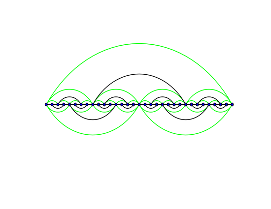
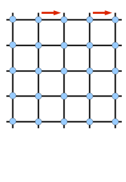
The hanoi networks (Boettcher et al., 2008, 2009; Boettcher and Brunson, 2011; Singh et al., 2014) possess a simple geometric backbone, a one-dimensional line of $N=2^{k}$ sites. Each site is at least connected to its nearest neighbor left and right on the backbone. To generate the small-world hierarchy in these networks, consider parameterizing any number $n<N$ (except for zero) uniquely in terms of two other integers $(i,j)$, $i\geq 1$ and $1\leq j\leq 2^{k-i}$, via

$$n = 2^{i-1}\left(2j-1\right).$$ (1)

Here, $i$ denotes the level in the hierarchy whereas $j$ labels consecutive sites within each hierarchy. To generate the network HN3, we connect each site $n=2^{i-1}(4j-3)$ also with a long-distance neighbor $n^{\prime}=2^{i-1}(4j-1)$ for $1\leq j\leq 2^{k-i-1}$, as shown in Fig. 1. While it is of a fixed, finite degree, we can extend HN3 in the following manner to obtain a new network of average degree 5, called HN5. In addition to the bonds in HN3, in HN5 we also connect all even sites to both of its nearest neighboring sites within the same level of the hierarchy $i\geq 1$ in Eq. (1). The resulting network remains planar but now sites have a hierarchy-dependent degree with an exponential degree distribution, also demonstrated in Fig. 1. Previously(Boettcher et al., 2008), it was found that the average chemical path between sites on HN3 scales as $d^{HN3}\sim\sqrt{N}$, reminiscent of a square-lattice consisting of $N$ lattice sites. In HN5, it is easy to show recursively that this distance grows as $d^{HN5}\sim\log_{2}N$ (Boettcher and Brunson, 2011).

Figure 1: Depiction of the Hanoi networks HN3 (black bonds only) and HN5 (black and green-shaded bonds).

II.2 Migdal-Kadanoff renormalization group

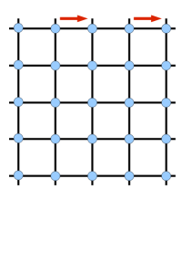
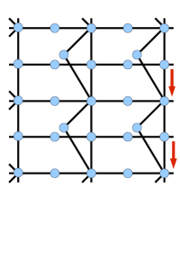
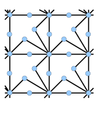
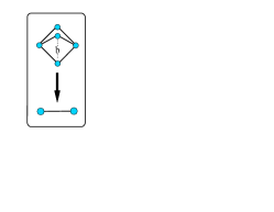
The Migdal-Kadanoff renormalization group (MKRG) (Migdal, 1976; Kadanoff, 1976; Berker and Ostlund, 1979) is a bond-moving scheme that approximates $d$-dimensional lattices. It often provides excellent approximations for $d=2$ and 3 (Southern and Young, 1977), and it becomes trivially exact in $d=1.$ The networks resulting from MKRG have a simple recursive, yet geometric, structure and have been widely studied in statistical physics (Fischer and Hertz, 1991; Plischke and Bergersen, 1994; Pathria, 1996). Starting from generation $\mu$ with a single bond, at each subsequent generation $\mu+1,$ all bonds are replaced with a new sub-graph. This structure of the sub-graph arises from the bond-moving scheme in $d$ dimensions (Migdal, 1976; Kadanoff, 1976), as depicted in Fig. 2: In a hyper-cubic lattice of unit bond length, at first all $l-1$ intervening hyper-planes of bonds, transverse to a chosen direction, are projected into every $l^{{\rm th}}$ hyper-plane, followed by the same step for $l-1$ hyper-planes being projected onto the $l^{{\rm th}}$ plane in the next direction, and so on. In the end, as shown in Fig. 3, one obtains a renormalized hyper-cubic lattice (of bond length $l)$ in generation $\mu+1$ with a renormalized bond of generation $\mu+1$ consisting of a sub-graph of

$$b=l^{d-1}$$ (2)

parallel branches, each having of a series of $l$ bonds of generation $\mu$. In turn, we can rewrite Eq. (2) as

$$d=1+\log_{l}b,$$ (3)

anticipating analytic continuation in $l$ and $b$ to obtain results for arbitrary, real dimensions $d$. In the following, we consider a general series of Migdal-Kadanoff networks by varying $b$ while fixing $l=2$.

Figure 2: Bond-moving scheme in the Migdal–Kadanoff renormalization group, here for a square lattice ($d=2$) with $l=2$, i. e. $b=2$ in Eq. (2). Starting from the lattice with unit bonds (a), bonds in intervening hyper-planes are projected onto every $l^{{\rm th}}$ plane in one direction while bonds connect to the $l^{{\rm th}}$ plane only at every $l^{{\rm th}}$ vertex (b), which is then repeated in subsequent directions (c), to re-obtain a similar hyper-cubic lattice, now of bond-length $l$ (d). The renormalized bonds in this case consist of $b=l^{d-1}=2$ branches, each of a series of $l=2$ bonds; the general RG-step for $l=2$ and arbitrary branches $b$ is depicted in Fig. 3

Figure 3: Hierarchical RG that results from the bond-moving scheme of any $d$-dimensional lattice shown in Fig. 2. A collection of $b$ strings of $l$ bonds at generation $\mu$ each ($l=2$ here) gets renormalized into a single new bond at generation $\mu+1$.

III Spectral Zeta-Functions of Laplacians

The Laplacian matrix is given by

$$\left[{\bf L}\right]_{i,j} = d_{i}\delta_{i,j}-A_{i,j},$$ (4)

where $d_{i}$ specifies the degree of the $i$-th vertex and $A_{i,j}$ is the adjacency matrix of the network. Since the links in the networks are undirected, ${\bf A}$ and ${\bf L}$ are symmetric. By design, all row or column sums in ${\bf L}$ vanish, i.e., $\sum_{i}\left[{\bf L}\right]_{i,j}=\sum_{j}\left[{\bf L}\right]_{i,j}=0$. The fundamental property of the Laplacian matrix is its spectrum of eigenvalues, the solutions $\lambda_{i}$ of the secular equation

$$\det\left[{\bf L}-\lambda{\bf 1}\right] = 0.$$ (5)

With an RG approach (Boettcher and Li, 2015), the effort of determining the spectrum reduces exponentially from solving $2^{k}\times 2^{k}$ determinants to $k$ iterations in a few RG recursion equations for any desired quantity.

We motivate our studies into the spectrum of the Laplacian matrix and their spectral zeta-functions through the intimate connection between various dynamic properties of transport phenomena and the geometry expressed via the Laplacian. In particular, it has been shown that the ratio between lowest and highest (nontrivial) eigenvalue provides a measure for the synchronization ability of coupled identical oscillators located on the nodes of the network(Barahona and Pecora, 2002). Another synchronization problem emerges in the context of parallel discrete-event simulations (PDES) (Korniss et al., 2003; Kozma et al., 2004), where nodes must frequently “synchronize” with their neighbors (on a given network) to ensure causality in the underlying simulated dynamics. The local synchronizations, however, can introduce correlations in the resulting synchronization landscape, leading to strongly nonuniform progress at the individual processing nodes. The above is a prototypical example for synchronization in many systems such as causally constrained queuing networks, supply-chain networks based on electronic transactions (Nagurney et al., 2005), etc.

Consider an arbitrary network in which the nodes interact through the links. The nodes are assumed to be task processing units, such as computers or manufacturing devices. Each node has completed an amount of task $h_{i}$ and these together at all nodes constitute the task-completion (synchronization) landscape $\{h_{i}(t)\}_{i=1}^{N}$. Here $t$ is the discrete number of parallel steps executed by all nodes, which is proportional to the real time, and $N$ is the number of nodes. In this particular model the nodes whose local field variables are incremented by an exponentially distributed random amount at a given step are those whose completed task amount is not greater than the tasks at their neighbors. Thus, denoting the neighborhood of the node $i$ by $S_{i}$, if $h_{i}(t)\leq\min_{j\in S_{i}}\{h_{j}(t)\}$, the node $i$ completes some additional exponentially distributed random amount of task; otherwise, it idles. In its simplest form the evolution equation for the amount of task completed at the node $i$ can be written as

$$h_{i}(t+1)=h_{i}(t)+\eta_{i}(t)\prod_{j\in S_{i}}\Theta\left(h_{j}(t)-h_{i}(t)\right),$$ (6)

where $h_{i}(t)$ is the local field variable (amount of task completed) at node $i$ at time $t$; $\eta_{i}(t)$ are iid random variables with unit mean, delta-correlated in space and time (the new task amount); and $\Theta(...)$ is the Heaviside step function. Despite its simplicity, this rule preserves unaltered the asynchronous dynamics of the underlying system. The larger the disparity in task completion is, the more memory has to be stored in the advanced units, which is costly in the context of limited resources. A measure of that cost, then, is the amount of de-synchronization, which is provided by the average “surface-roughness”

$$\left\langle w^{2}\right\rangle = \frac{1}{N}\sum_{i=2}^{N}\frac{1}{\lambda_{i}},$$ (7)

where $\lambda_{i}$ are the rank-ordered eigenvalues of the Laplacian matrix ${\bf L}$ of the network, leaving out the trivial, lowest eigenvalue $\lambda_{1}=0$. It is very difficult to analytically calculate each eigenvalue individually to evaluate the sum defining $\left\langle w^{2}\right\rangle$ in Eq. (7).

As similar problem is encountered in the evaluation of the efficiency of quantum search on a network (Childs and Goldstone, 2004). However, in this case, we need to access even higher moments of the eigenvalues. So, it becomes useful to define an entire function generating such moments:

$$I_{j}=\frac{1}{N}\,\sum_{i=2}^{N}\left(\frac{1}{\lambda_{i}}\right)^{j},$$ (8)

the spectral zeta-function (Voros, 1992; Akkermans et al., 2009; Dunne, 2012). Note, for instance, that in the evaluation of partition functions in field theory the $I_{j}$ often feature in the continuation to non-integer moments, in particular, the limit $j\to 0$ (Ramond, 1997). In almost all cases, with the exception of regular lattices where Fourier transforms can be applied, and some fractals (Rammal, 1984), it is impossible to find each eigenvalue in the sum of Eq. (8). However, the sum defined in Eq. (8) for $I_{j}$ can be expressed as the $j^{{\rm th}}$ derivative of the determinant ${\bf\mathbf{\mathcal{L}}}+\epsilon\mathbb{I}$ in the limit $\epsilon\to 0$:

$$I_{j} = \frac{1}{N}\,\left.\frac{\left(-1\right)^{j-1}}{\left(j-1\right)!}\left(\frac{\partial}{\partial\epsilon}\right)^{j}\,\sum_{i=2}^{N}\ln\left(\lambda_{i}+\epsilon\right)\right|_{\epsilon\to 0},$$ (9)

$$= \frac{1}{N}\,\left.\frac{\left(-1\right)^{j-1}}{\left(j-1\right)!}\left(\frac{\partial}{\partial\epsilon}\right)^{j}\,\ln\left[\frac{1}{\epsilon}\prod_{i=1}^{N}\left(\lambda_{i}+\epsilon\right)\right]\right|_{\epsilon\to 0},$$

$$= \frac{1}{N}\,\left.\frac{\left(-1\right)^{j-1}}{\left(j-1\right)!}\left(\frac{\partial}{\partial\epsilon}\right)^{j}\,\ln\left[\frac{1}{\epsilon}\det\left({\bf L}+\epsilon{\bf 1}\right)\right]\right|_{\epsilon\to 0},$$

where we have used the fact that $\lambda_{1}=0$. This has the advantage that we do not need to know each individual Laplacian eigenvalue $\lambda_{i}$, as has been previously assumed in the context of quantum search and many other applications(Agliari et al., 2010; Agliari and Tavani, 2017). Note, for instance, that Eq. (7) now reduces to $\left\langle w^{2}\right\rangle=I_{1}$. In the following, we can take advantage of the RG-techniques developed for Laplacian determinants in Ref. (Boettcher and Li, 2015) to derive the scaling of $I_{j}$.

III.1 A Heuristic Argument

Figure 4: Plot of the Laplacian eigenvalues $\lambda_{i}$ ordered by rank $i$ as a function of $\frac{i}{N}$ for various system sizes $N$ of the Hanoi network HN3 (left) and MKRG at $b=3$ (right). The dashed line follows a power law with exponent $2/d_{s}=d_{w}/d_{f}\approx 1.31$ (Boettcher and Gonçalves, 2008) for HN3, and for MKRG with $d_{s}=1+\log_{2}3$. The inset for HN3 shows the same data for only $N=2^{16}$ on a linear scale, showing that the scaling concerns only the part of the spectrum where $\frac{i}{N}$ is small. While the assumptions underlying Eq. (10) seem well-justified for HN3, the high degree of degeneracy in MKRG spectra makes the heuristic argument in Sec. III.1 more dubious, and progressively worse for larger $b$.

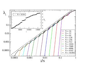
If we assume (Rammal, 1984) that the rank-ordered eigenvalues $0=\lambda_{1}<\lambda_{i}\leq\lambda_{i_{c}}$ for all $2\leq i\leq i_{c}$ up to some $2\leq i_{c}\leq N$ for large $N$ follow a power-law form,

$$\lambda_{i}\sim\left(\frac{i}{N}\right)^{\frac{2}{d_{s}}},$$ (10)

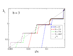
and $\lambda_{i}\sim const$ for $i>i_{c}$. This is shown, for instance, in Fig. 4 to be applicable for the fractal network HN3, for which $2/d_{s}=d_{w}/d_{f}=2-\log_{2}\phi\approx 1.31$ with $\phi=\left(\sqrt{5}+1\right)/2$ (Boettcher and Gonçalves, 2008), but it is at best vaguely satisfied for MKRG even in the best-case scenario, $b=3$, because of an ever higher degree of degeneracy in the spectrum. Note that under these assumptions, it is in fact easy to evaluate the spectral zeta-function in Eq. (8) directly by taking the Riemann limit, $\frac{i}{N}\to\theta$ with $d\theta=\frac{1}{N}$, such that

$$\frac{1}{N}\,\sum_{i=2}^{N}\left(\frac{1}{\lambda_{i}}\right)^{j} \sim \int_{\frac{1}{N}}^{\theta_{c}}d\theta\,\theta^{-\frac{2j}{d_{s}}}+const,$$ (11)

$$\sim N^{\frac{2j}{d_{s}}-1}+const.$$

This result would hold for any $\theta_{c}=\frac{i_{c}}{N}\sim N^{-\nu}$ with $0\leq\nu<1$, such that the $N$-dependent scaling is dominated by the lower limit of the integral.

IV RG for the Spectral Determinant of Hanoi Networks

The determinant of ${\cal L}(\epsilon)={\bf L}+\epsilon{\bf 1}$ in Eq. (9) for fractal lattices can be evaluated asymptotically in a recursive renormalization scheme. We have already described the procedure in great detail in Ref. (Boettcher and Li, 2015). Here we only outline the procedure to be able to focus on the novel aspects need for our calculation here. In general, we employ the well-known formal identity (Ramond, 1997),

$$\frac{1}{\sqrt{\det{\cal L}}} = \idotsint_{-\infty}^{\infty}\left(\prod_{i=1}^{N}\frac{dx_{i}}{\sqrt{\pi}}\right)\exp\left\{-\sum_{n=1}^{N}\sum_{m=1}^{N}x_{n}{\cal L}_{n,m}x_{m}\right\}.$$ (12)

For the RG, we employ a hierarchical scheme by which at each step $\mu$ a fraction $1/b$ of all remaining variables get integrated out while leaving the integral in Eq. (12) invariant, but now with $N^{\prime}\leq N/b$ variables. Formally, say, in case of $b=2$ we integrate out every odd-indexed variable in a network at step $\mu$, we separate $\prod_{i=1}^{N}dx_{i}=\prod_{i=1}^{N/2}dx_{2i}\prod_{j=1}^{N/2}dx_{2j+1}$ and integrate to receive

$$\frac{1}{\sqrt{\det{\cal L}}}=C^{\prime}\idotsint_{-\infty}^{\infty}\left(\prod_{i=1}^{\frac{N}{2}}\frac{dx_{2i}}{\sqrt{\pi}}\right)\exp\left\{-\sum_{n=1}^{\frac{N}{2}}\sum_{m=1}^{\frac{N}{2}}x_{2n}{\cal L}_{n,m}^{\prime}x_{2m}\right\},$$ (13)

where the reduced Laplacian ${\cal L}^{\prime}$ is now a $\frac{N}{2}\times\frac{N}{2}$ matrix that is formally identical with ${\cal L}$ and $C^{\prime}$ is an overall scale-factor. That is, if ${\cal L}={\cal L}\left(q,p,\ldots\right)$ depends on some parameters, then ${\cal L}^{\prime}={\cal L}^{\prime}\left(q^{\prime},p^{\prime},\ldots\right)$ depends on those parameters in the same functional form, thereby revealing the RG-recursion relations, $q^{\prime}=q^{\prime}\left(q,p,\ldots\right)$, $p^{\prime}=p^{\prime}\left(q,p,\ldots\right)$, etc, and $C^{\prime}=C^{\prime}\left(q,p,\ldots\right)$, that encapsulate all information of the original Laplacian. After a sufficient number of such RG-steps, a reduced Laplacian of merely a few variables remains that can be solved by elementary means. This property, of course, is very special and can be iterated in exact form only for certain types of fractal networks.

In Ref. (Boettcher and Li, 2015), we have shown, for example, that for the Hanoi networks HN3 and HN5 we find the RG recursions:

$$q_{\mu+1} = q_{\mu}+2l_{\mu}-2\frac{p_{\mu}^{2}}{q_{\mu}-1},$$

$$p_{\mu+1} = l_{\mu}+\frac{p_{\mu}^{2}}{q_{\mu}-1},$$ (14)

$$l_{\mu+1} = l_{0}+\frac{p_{\mu}^{2}}{q_{\mu}^{2}-1},$$

and

$$C_{k}^{(\mu)} = \prod_{i=0}^{\mu-1}\left[q_{i}^{2}-1\right]^{-2^{k-3-i}},$$ (15)

such that the determinant of the Laplacian after $k-2$ RG-steps becomes:

$$\det\left[{\bf{\bf L}_{k}^{(3,5)}}+\epsilon{\bf 1}\right] \sim \epsilon\left[C_{k}^{(k-2)}\right]^{-2}.$$ (16)

Note that the termination condition for the final RG-step merely contribute a factor of $\sim\epsilon$ that is needed to cancel the $1/\epsilon$ in Eq. (9) due to the $\lambda_{1}=0$-eigenvalue. The asymptotic behavior of the determinant itself arises entirely from $C_{k}^{(k-2)}$. Only the initial conditions on the RG-recursions distinguish between HN3 and HN5. These are:

$$C_{k}^{(0)} = 1,$$

$$q_{0} = 3+\epsilon,$$ (17)

$$p_{0} = 1,$$

$$l_{0} = \begin{cases}0,&{\rm for\,\,HN3}\\ 1,&{\rm for\,\,HN5}\end{cases}.$$

As shown in Ref. (Boettcher and Li, 2015) (and easily verified by insertion), the parameters $\left\{q_{k-2},p_{k-2},l_{k-2}\right\}$ in Eq.(14) in HN3 approach fixed points as

$$q_{\mu} \sim 1+\left(\frac{2}{\phi}\right)^{-\mu}\left(Q_{0}+\epsilon\left(\frac{4}{\phi}\right)^{\mu}Q_{1}+\epsilon^{2}\left(\frac{4}{\phi}\right)^{2\mu}Q_{2}\ldots\right),$$

$$p_{\mu} \sim\left(\frac{2}{\phi}\right)^{-\mu}\left(P_{0}+\epsilon\left(\frac{4}{\phi}\right)^{\mu}P_{1}+\epsilon^{2}\left(\frac{4}{\phi}\right)^{2\mu}P_{2}\ldots\right),$$ (18)

$$l_{\mu} \sim\left(\frac{2}{\phi}\right)^{-\mu}\left(L_{0}+\epsilon\left(\frac{4}{\phi}\right)^{\mu}L_{1}+\epsilon^{2}\left(\frac{4}{\phi}\right)^{2\mu}L_{2}\ldots\right),$$

where $\phi=\left(\sqrt{5}+1\right)/2$. In turn, the set of parameters in Eq.(14) for HN5 approach the fixed points as

$$q_{\mu} \sim\frac{5+\sqrt{41}}{2}+\left(\epsilon 2^{\mu}Q_{1}+\epsilon^{2}2^{2\mu}Q_{2}\ldots\right),$$

$$p_{\mu} \sim\frac{3+\sqrt{41}}{4}+\left(\epsilon 2^{\mu}P_{1}+\epsilon^{2}2^{2\mu}P_{2}\ldots\right),$$ (19)

$$l_{\mu} \sim\frac{3+\sqrt{41}}{8}+\left(\epsilon 2^{\mu}L_{1}+\epsilon^{2}2^{2\mu}L_{2}\right).$$

When Eq. (16) is evaluated for HN3, the overall factor $C_{k}^{\left(k-2\right)}$ is approximated using $q_{\mu}$ in Eq. (18),

$$C_{k}^{(\mu)} \sim \alpha^{N}\prod_{i=0}^{\mu-1}\left[\left(1+\left(\frac{2}{\phi}\right)^{-i}\left(Q_{0}+\epsilon\left(\frac{4}{\phi}\right)^{i}Q_{1}+\epsilon^{2}\left(\frac{4}{\phi}\right)^{2i}Q_{2}\ldots\right)\right)^{2}-1\right]^{-2^{k-3-i}},$$ (20)

in which the parameter $\alpha$ is determined to any accuracy by simple iteration of the recursions in Eq. (14), which was executed in Ref. (Boettcher and Li, 2015). For HN3, $\alpha=2.0189990298\ldots$; for HN5, $\alpha=2.7548806715\ldots$. However, the existence of the factor $\alpha^{N}$ is irrelevant for the scaling of $I_{j}$ since it has no contribution to the derivative of the logarithm of the determinant with respect to $\epsilon$. Applying Eq. (9), the zeta functions for HN3 eventually read as

$$I_{j} \sim \left[\left(\frac{2}{\phi}\right)^{\log_{2}N}\right]^{j},$$ (21)

$$\sim \left[N^{1-\log_{2}\phi}\right]^{j}.$$

Similarly, inserting $q_{i}$ in Eq. (19) into Eqs. (15-16) provides for HN5:

$$I_{j} \sim \begin{cases}\begin{array}[]{c}\log_{2}N\\ N^{2j/2-1}\end{array}&\begin{array}[]{c}j=1,\\ j\geq 2.\end{array}\end{cases}$$ (22)

For HN3 at $j=1$ in Eq. (21), it is easy to identify the exponent as $1-\log_{2}\phi=d_{w}-d_{f}$, in which $d_{w}=2-\log_{2}\phi$ is the random walk dimension obtained for HN3 in Ref. (Boettcher and Gonçalves, 2008) in the metric where the $1d$-backbone defines distances such that $d_{f}=1$. The results for the spectral zeta-function is consistent with that found generally by Ref. (Giacometti et al., 1995),

$$\left\langle w^{2}\right\rangle\sim L^{d_{w}-d_{f}},$$ (23)

for the surface roughness defined in Eq. (7) for which we have shown in Sec. III that $I_{1}=\left\langle w^{2}\right\rangle$. Using $d_{w}=2d_{f}/d_{s}$ (Alexander and Orbach, 1982) and the definition $N=L^{d_{f}}$ then leads to

$$I_{j}\sim N^{\frac{2j}{d_{s}}-1},$$ (24)

for $d_{s}<2j$, uniquely described in terms of the spectral dimension. For HN5, the spectral dimension is $d_{s}=2$, leading to the logarithmic scaling in Eq. (22) for $j=1$ where $d_{s}\geq 2j$. When $j\geq 2$, Eq. (24) also applies to HN5.

Figure 5: Graph-let for the MKRG for the spectral zeta-function, as adapted from the generic structure shown in Fig. 3. In that graph-let, the $b$ inner vertices $y_{1},\ldots,y_{b}$ belong to the currently lowest level ($i=0$) of the hierarchy that will be integrated out (${\bf\times}$-mark) in the next RG-step. One of the two outer vertices, $z$, must be exactly one level higher ($i=1$, here shown right). The other outer vertex, $x$, must be of some unspecified but higher level ($i>1$, left). After the RG-step, symbolized by the arrow, the renormalized link $B_{i-1}^{\prime}$ is bound to have a vertex $z$ with $i=0$ on one end and some vertex $x$ with $i^{\prime}=i-1>0$ on the other. A set of $2b$ of these links then become the input of the – identical – next RG-step.

V RG for the Spectral Determinant of Migdal-Kadanoff

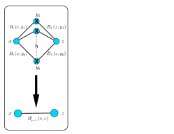
Since we have not considered MKRG before in this way, we derive its RG-recursions here in more detail. To this end, we can reconstruct the integral in Eq. (12) piece-by-piece by defining a simple algebra. As suggested by Fig. 2(c), in each RG-step the lattice consists of a collection of graph-lets of the type shown in Fig. 3, which we have adapted for the following calculation in Fig. 5. In that graph-let, the $b$ inner vertices belong to the currently lowest level ($i=0$) of the hierarchy that will be integrated out in the next RG-step. One of the two outer vertices is exactly one level higher ($i=1$) as it would be integrated at the next step. The other outer vertex must be of some unspecified but higher level ($i>1$). We can now define a helpful function pertaining to each bond, each of which is bound to have a vertex with $i=0$ on one end and some vertex with $i>0$ on the other. Its part of the integrand in Eq. (12) has the form

$$B_{i}\left(x,y\right)=C_{i}\exp\left\{-\frac{q_{i}}{2}x^{2}-\frac{q_{0}}{2}y^{2}+2pxy\right\},$$ (25)

such that the RG-step depicted in Fig. 2(d) amounts to

$$B_{i-1}^{\prime}\left(x,z\right) = \idotsint_{-\infty}^{\infty}\prod_{j=1}^{b}\frac{dy_{j}}{\sqrt{\pi}}\,B_{i}\left(x,y_{j}\right)B_{1}\left(z,y_{j}\right),$$ (26)

$$= C_{i}^{b}C_{1}^{b}\exp\left\{-\frac{b}{2}\left(q_{i}x^{2}+q_{1}z^{2}\right)\right\}\idotsint_{-\infty}^{\infty}\prod_{j=1}^{b}\frac{dy_{j}}{\sqrt{\pi}}\,\exp\left\{-q_{0}y_{j}^{2}+2p\left(x+z\right)y_{j}\right\},$$

$$= C_{i}^{b}C_{1}^{b}q_{0}^{-\frac{b}{2}}\exp\left\{-\frac{b}{2}\left(q_{i}-\frac{2p^{2}}{q_{0}}\right)x^{2}-\frac{b}{2}\left(q_{1}-\frac{2p^{2}}{q_{0}}\right)z^{2}+2b\frac{p^{2}}{q_{0}}xz\right\},$$

$$= C_{i-1}^{\prime}\exp\left\{-\frac{q_{i-1}^{\prime}}{2}x^{2}-\frac{q_{0}^{\prime}}{2}z^{2}+2p^{\prime}xz\right\},$$

where unprimed parameters are $\mu$-times previously renormalized while primes indicate newly $\mu+1$-times renormalized parameters. From the last two lines, we can read off the RG-recursions at the $\mu^{{\rm th}}$ step:

$$C_{i-1}^{(\mu+1)} = \left(\frac{C_{1}^{(\mu)}C_{i}^{(\mu)}}{\sqrt{q_{0}^{(\mu)}}}\right)^{b},$$

$$q_{i-1}^{(\mu+1)} = b\,\left(q_{i}^{(\mu)}-\frac{2\left(p^{(\mu)}\right)^{2}}{q_{0}^{(\mu)}}\right),$$ (27)

$$p^{(\mu+1)} = b\,\frac{\left(p^{(\mu)}\right)^{2}}{q_{0}^{(\mu)}},$$

for $i>0$. Considering that initially, at $\mu=0$ in the unrenormalized network, all vertex-weights defined in Eq. (25) are the same, $q_{i}^{(0)}\equiv 2$ for all $i$, the distinction between levels $i$ in Eq. (27) disappears. Note that a vertex at level $i>0$ contributes to the Gaussian integral $2b^{i}$-fold through respective factors $B_{i}$, and 2-fold for $i=0$ by appearing in two such factors $B_{i^{\prime}}$, $i^{\prime}>0$. In this manner, the lattice Laplacian at $\mu=0$ in Eq. (12) receives its proper weights on its diagonal. Equally, $C_{i}^{(0)}=1$ for all $i>0$. Thus, defining $C_{\mu}=C_{i}^{(\mu)}$, $p_{\mu}=b^{-\mu}p^{(\mu)}$, and $q_{\mu}=b^{-\mu}q_{i}^{(\mu)}$ for all $i\geq 0$, we obtain:

$$C_{\mu+1} = \left[\frac{C_{\mu}^{2}}{\sqrt{b^{\mu}q_{\mu}}}\right]^{b},\qquad\left(C_{0}=1\right),$$

$$q_{\mu+1} = q_{\mu}-2\frac{p_{\mu}^{2}}{q_{\mu}},\qquad\left(q_{0}=2-\epsilon\right),$$ (28)

$$p_{\mu+1} = \frac{p_{\mu}^{2}}{q_{\mu}},\qquad\left(p_{0}=1\right).$$

Note that the recursions in Eq. (28) is not exactly identical to Eq. (27). With eigenvalue $\lambda=-\epsilon$, the initial condition for $q_{i}^{\left(0\right)}$ Eq. (27) is, in fact,

$$q_{i}^{\left(0\right)} = 2+\epsilon/b^{i},\qquad 0\leq i<k,$$ (29)

$$q_{k}^{\left(0\right)} = 2+2\epsilon/b^{k},\qquad i=k,$$

which does not allow to collapse the $i$-th hierarchy like in the Hanoi networks. However, in the Taylor expansion in small $\epsilon$, order-by-order such a collapse is allowed. The difference between the $\left\{q_{0}^{\left(\mu\right)},p^{\left(\mu\right)}\right\}$ from Eq. (28) and $\left\{q_{\mu},p_{\mu}\right\}$ from Eq. (27) is

$$q_{0}^{\left(\mu\right)}-q_{\mu} \sim Q_{1}\epsilon+Q_{2}\epsilon^{2}+Q_{3}\epsilon^{3}+\ldots,$$ (30)

$$p^{\left(\mu\right)}-p_{\mu} \sim P_{1}\epsilon+P_{2}\epsilon^{2}+P_{3}\epsilon^{3}+\ldots$$ (31)

in which coefficients are all constants dependent only on the parameter $b$. After $k-1$ iterations, the network is renormalized to two end nodes, the Laplacian determinant is

$$\det\left[{\bf{\bf L}_{k}^{MK}}+\epsilon{\bf 1}\right] = C_{k}^{-2}b^{2k}\,\det\left[\begin{array}[]{cc}q_{k}/2&-p_{k}\\ -p_{k}&q_{k}/2\end{array}\right]$$ (34)

$$= C_{k}^{-2}b^{2k}\left(q_{k}^{2}/4-p_{k}^{2}\right),$$ (35)

where the $C_{k}^{-2}$ can be expressed in closed form,

$$C_{k}^{-2} = \left(b^{0}q_{0}\right)^{2^{k-1}b^{k}}\left(b^{1}q_{1}\right)^{2^{k-2}b^{k-1}}\left(b^{2}q_{2}\right)^{2^{k-3}b^{k-2}}\ldots\left(b^{k-1}q_{k-1}\right)^{2^{k-k}b}$$

$$= \left(\prod_{\mu=0}^{k-1}b^{\left(2b\right)^{k-\mu}\thinspace\mu/2}\right)\left(\prod_{\mu=0}^{k-1}q_{\mu}^{b\thinspace\left(2b\right)^{k-1-\mu}}\right).$$

The ansatz for fixed points of rescaled $\left\{q_{\mu},p_{\mu}\right\}$ in Eq. (28) is

$$q_{\mu} \sim 2^{-\mu}\left(Q_{0}+\epsilon 4^{\mu}Q_{1}+\epsilon^{2}4^{2\mu}Q_{2}\ldots\right),$$

$$p_{\mu} \sim 2^{-\mu}\left(Q_{0}/2-\epsilon 4{}^{\mu}P_{1}/4+\epsilon^{2}4^{2\mu}P_{2}+\ldots\right).$$ (36)

The fixed point scaling of parameters $q_{\mu}$ and $p_{\mu}$ in Eq. (36) verifies the validity of approximations in Eq. (28), since the differences between the approximated and exact parameters in Eq. (30) will not affect the scaling of any quantity we consider in Eq. (9). With respect to $\epsilon$, we can calculate the $j^{{\rm th}}$ derivative of determinant for any $b$. Note that the asymptotic expression for $\left[C_{k}^{(k-1)}\right]^{-2}$ is approximated to

$$C_{k}^{-2} \sim\alpha^{N} \prod_{\mu=0}^{k-1}\left[q_{\mu}\right]^{b\thinspace\left(2b\right)^{k-1-\mu}},$$

in which $\alpha$ is determined respectively as $1.0594630943\ldots$, $1.0233738919\ldots$, $1.0124545480\ldots$, $1.0077313692\ldots$, and $1.0052649262\ldots$ for $b=2,3,4,5,6$. As argued above, however, any such $\epsilon$-independent factor remains irrelevant after the differentiation in Eq. (9).

The zeta-functions for the Laplacian determinants with varying $b$ are eventually evaluated as

$$I_{j} \sim \begin{cases}\begin{array}[]{c}N^{2j/(1+\log_{2}b)-1}\\ \ln N\\ const\end{array}&\begin{array}[]{c}2j>(1+\log_{2}b)\\ 2j=(1+\log_{2}b)\\ 2j<(1+\log_{2}b)\end{array}\end{cases}$$ (37)

Considering that the spectral dimensions for MKRG with $l=2$(Akkermans et al., 2009) are

$$d_{s} =d= 1+\log_{2}b,$$ (38)

the zeta-functions are again identified as

$$I_{j} \sim N^{2j/d_{s}-1},\qquad 2j>d_{s},$$ (39)

as in Eq, (24).

VI Conclusion

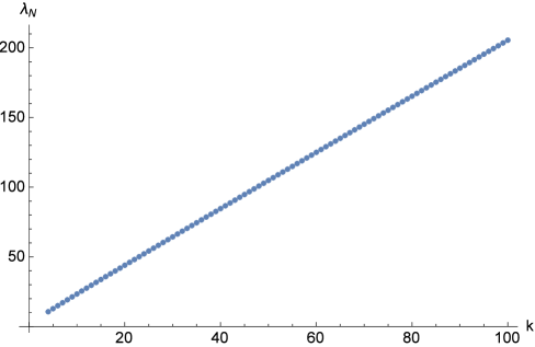
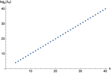
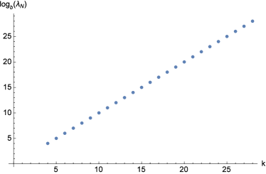
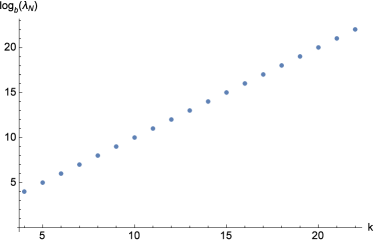
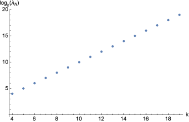
We have calculated the exact asymptotic scaling of spectral zeta-functions for Hanoi networks and MKRG using the renormalization group. The results highlight the importance of the spectral exponent $d_{s}$ for many physical applications, such as synchronization and quantum searches. For example, in Ref. (Li and Boettcher, to appear, arXiv:1607.05317), we use Eq. (24) to show that the efficiency of continuous-time quantum walks is controlled by $d_{s}$ for any network, which generalizes the results previously obtained for hyper-cubic lattices (Childs and Goldstone, 2004). Synchronization of identical dynamical systems in a network has been shown in Ref. (Barahona and Pecora, 2002) to depend on the scaling of the eigenratio of largest to smallest nonzero eigenvalue of the network Laplacian. From our analysis in Sec. IV and Sec. V, the smallest nonzero eigenvalue $\lambda_{2}>0$ can be approximated by $I_{1}$, when $d_{s}<2$ is satisfied. It is also suggested by the argument in Sec. III.1. For HN3, a degree-3 network, the largest eigenvalue is bounded above by $\lambda_{N}\leq 6$, and it is interesting to show (in the Appendix) how to use RG with the “power method” (Kuczynski and Wozniakowski, 1992) for matrices to find that, in fact, $\lambda_{N}=5.37272879308215\ldots$. The same arguments are applied to HN5, for which the asymptotic value of $\lambda_{N}$ evolved with the numerical power method for varying size $N=2^{k}$ is presented in Fig. 6. The largest eigenvalues are shown to scale with $\lambda_{N}\sim 2\log_{2}N$. This method also allows us to obtain the asymptotic value of $\lambda_{N}$ for hierarchical networks from MKRG, which scales as $\lambda_{N}\sim b^{k}\sim N$, shown in Fig. 7.

The calculation on the smallest nonzero and largest eigenvalue $\lambda_{2}$ and $\lambda_{N}$ allows us to analyze the synchronizability of all the relevant networks. The linear stability of the synchronous state is related to an algebraic condition of the Laplacian matrix according to Ref. (Barahona and Pecora, 2002). The generic requirement for the synchronous state to be linearly stable is $\sigma\lambda_{i}\in\left(\alpha_{1},\alpha_{2}\right)$ for all the nonzero eigenvalues of the Laplacian matrix, where $\sigma$ is the globle coupling, and $\left(\alpha_{1},\alpha_{2}\right)$ is the negative region of the master stability function that depends solely on the dynamical system. For dynamical systems on network of arbitrary topology, whether the network is synchronizable is decided by the algebraic condition $\lambda_{N}/\lambda_{2}<\alpha_{2}/\alpha_{1}(=const)$. This eigenratio determines the synchronizability of a network. The eigenratios of HN3, HN5 and MKRG are asymptotically $N^{2-\log_{2}\phi}$,$2N\log_{2}N$ and $N^{\left(3+\log_{2}b\right)/\left(1+\log_{2}b\right)}$. This would imply that the synchronizability for these networks is ranked as HN5>HN3>MKRG, as long as $d_{s}<2/\left(1-\log_{2}\phi\right)\approx 6.54$ (or $b<46.5$).

Acknowledgements:

We acknowledge financial support from the U. S. National Science Foundation through grant DMR-1207431.

Figure 6: Plot of the largest eigenvalue $\lambda_{N}$ for HN5 with system size $k\left(=\log_{2}N\right)$, as obtained by the power-method using the recursions in Eq. (51) . A linear fit provides a scaling of $\lambda_{N}\sim 2.023588046\ldots k+3.460393100\ldots$.

(a) b=2

(b) b=3

(c) b=4

(d) b=5

Figure 7: Plots of the largest eigenvalue $\lambda_{N}$ with system size $k(\sim\log_{b}N)$ for MKRG with $b=2,3,4,5$. It can be fitted respectively as $\log_{b=2}\lambda_{N}=0.9992544987\ldots k+0.0213953207\ldots$, $\log_{b=3}\lambda_{N}=0.9998501326\ldots k+0.0030754291\ldots$, $\log_{b=4}\lambda_{N}=0.9999427813\ldots k+0.0009418968\ldots$, and $\log_{b=5}\lambda_{N}=0.9999734834\ldots k+0.0003826594\ldots$, showing that $\lambda_{N}\sim b^{k}\sim N$.

Appendix:

VI.1 Largest Eigenvalue

We can use the power method, commonly used to numerically extract particular eigenvalues of a matrix, to obtain the largest eigenvalue of the Laplacian for HN3 analytically. The power method simply proceeds as follows: Choose any generic vector ${\bf x}_{0}$ (that is non-zero and not already an eigenvector associated with another eigenvalue), then the evolution of

$${\bf x}_{t+1} = \frac{1}{\bar{\lambda}_{t}}{\bf L}{\bf x}_{t},$$ (40)

converges to the eigenvector associated with the (absolute) largest eigenvalue (if unique) of any matrix ${\bf M}$, where

$$\bar{\lambda_{t}} = \left\|{\bf x}_{t}\right\|$$ (41)

ensures proper normalization of the evolving vector ${\bf x}_{t}$. The magnitude of that largest eigenvalue is provided by $\lambda_{N}=\lim_{t\to\infty}\bar{\lambda}_{t}$. Hence, analytically, we are faced with solving the fixed point equation

$${\bf x}^{*} = \frac{1}{\lambda_{N}}{\bf L}{\bf x}^{*},$$ (42)

which is typically hopeless in general. But in case of the very sparse, hierarchical Laplacian matrix for HN3, the set of $N=2^{k}$ coupled linear equations defined by Eq. (42) can be solved again recursively. Then, we can write for Eq. (42):

$$0 = \left(3-\lambda_{N}\right)x_{0}-x_{2^{k}-1}-x_{1}-x_{2^{k-1}},$$

$$0 = \left(3-\lambda_{N}\right)x_{2^{k-1}}-x_{2^{k-1}-1}-x_{2^{k-1}+1}-x_{0},$$ (43)

$$0 = \left(3-\lambda_{N}\right)x_{2^{i-1}(4j-3)}-x_{2^{i-1}(4j-3)-1}-x_{2^{i-1}(4j-3)+1}-x_{2^{i-1}(4j-1)},$$

$$0 = \left(3-\lambda_{N}\right)x_{2^{i-1}(4j-1)}-x_{2^{i-1}(4j-1)-1}-x_{2^{i-1}(4j-1)+1}-x_{2^{i-1}(4j-3)},$$

for all $1\leq i<k$ and $1\leq j\leq 2^{i-2}$. The recursion consists of solving for and eliminating all odd-index ($i=1$) variables. To that end, we re-write Eqs. (43) as

$$0 = q_{2}\,x_{n-2}-p\left(x_{n-3}+x_{n-1}\right)-l\left(x_{n-4}+x_{n}\right)-x_{+},$$

$$0 = q_{1}\,x_{n-1}-p\left(x_{n-2}+x_{n}\right)-x_{n+1},$$ (44)

$$0 = q_{2}\,x_{n}-p\left(x_{n-1}+x_{n+1}\right)-l\left(x_{n-2}+x_{n+2}\right)-x_{n\pm 4},$$

$$0 = q_{1}\,x_{n+1}-p\left(x_{n+2}+x_{n}\right)-x_{n-1},$$

$$0 = q_{2}\,x_{n+2}-p\left(x_{n+3}+x_{n+1}\right)-l\left(x_{n+4}+x_{n}\right)-x_{-},$$

for all $n=2(2j-1)$, $j=1,\ldots,2^{k-2}$, where initially

$$q_{1}^{(0)}=q_{2}^{(0)} = 3-\lambda_{N},$$

$$p^{(0)} = 1,$$ (45)

$$l^{(0)} = 0.$$

Solving for and eliminating all odd-indexed variables $x_{n\pm 1}$, we find

$$0 = \left(q_{2}-\frac{2p^{2}q_{1}}{q_{1}^{2}-1}\right)\,x_{n-2}-\left(l+\frac{p^{2}}{q_{1}-1}\right)\left(x_{n-3}+x_{n-1}\right)-\frac{p^{2}}{q_{1}^{2}-1}\left(x_{n-4}+x_{n}\right)-x_{+},$$

$$0 = \left(q_{2}-\frac{2p^{2}}{q_{1}-1}\right)\,x_{n}-\left(l+\frac{p^{2}}{q_{1}-1}\right)\left(x_{n-2}+x_{n+2}\right)-x_{n\pm 4},$$ (46)

$$0 = \left(q_{2}-\frac{2p^{2}q_{1}}{q_{1}^{2}-1}\right)\,x_{n+2}-\left(l+\frac{p^{2}}{q_{1}-1}\right)\left(x_{n+3}+x_{n+1}\right)-\frac{p^{2}}{q_{1}^{2}-1}\left(x_{n+4}+x_{n}\right)-x_{-}.$$

Similar to the renormalization group treatment of HN3 in Sect. IV, we relabel $x^{\prime}_{n^{\prime}+2}=x_{n+2}$, $x^{\prime}_{n^{\prime}+1}=x_{n}$, and $x^{\prime}_{n^{\prime}}=x_{n-2}$, and obtain

$$q^{\prime}_{1} = q_{2}-\frac{2p^{2}}{q_{1}-1},$$

$$q^{\prime}_{2} = q_{2}-\frac{2p^{2}q_{1}}{q_{1}^{2}-1},$$

$$p^{\prime} = l+\frac{p^{2}}{q_{1}-1},$$ (47)

$$l^{\prime} = \frac{p^{2}}{q_{1}^{2}-1},$$

considering which should be compared with Eqs. (14). Then, Eqs. (46) in terms of the primed quantities take on exactly the form of the (lower three) Eqs. (44) and the circle closes. The recursion terminates after $k-2$ steps with the equations

$$0 = q_{2}^{(k-2)}\,x_{0}-p^{(k-2)}\left(x_{1}+x_{3}\right)-\left(2l^{(k-2)}+1\right)x_{2},$$

$$0 = q_{1}^{(k-2)}\,x_{1}-p^{(k-2)}\left(x_{0}+x_{2}\right)-x_{3},$$ (48)

$$0 = q_{2}^{(k-2)}\,x_{2}-p^{(k-2)}\left(x_{1}+x_{3}\right)-\left(2l^{(k-2)}+1\right)x_{0},$$

$$0 = q_{1}^{(k-2)}\,x_{3}-p^{(k-2)}\left(x_{0}+x_{2}\right)-x_{1},$$

which lead to the constraint

$$0 = q_{2}^{(k-2)}-2l^{(k-2)}+1.$$ (49)

Combining Eqs. (45), (47), and (49) provide an efficient procedure to determine the largest eigenvalue $\lambda_{N}$, albeit implicit. For instance, for $k=2$, we can directly insert Eqs. (45) into Eq. (49) to find $\lambda_{4}=4$, for $k=3$, we recur the initial conditions in Eqs. (45) once through Eqs. (47) before we apply the constraint in Eq. (49) to get

$$0 = \left(3-\lambda_{8}\right)-\frac{2\left(3-\lambda_{8}\right)}{\left(3-\lambda_{8}\right)^{2}-1}+\frac{2}{\left(3-\lambda_{8}\right)^{2}-1}+1$$

with the solution $\lambda_{8}=4+\sqrt{2}=5.414\ldots$. Beyond that, a closed-form solution becomes quite difficult, and we have to resort to an implicit “shooting” procedure, which is nonetheless exponentially more efficient, $O(k=\log_{2}N)$, than a numerical evaluation with the power method: simply choose a trial value for $\lambda_{N}$ in Eqs. (45) and evolve the recursion in Eqs. (47) until the right-hand side of Eq. (49) has sufficiently converged, then vary the value of $\lambda_{N}$ (using bisectioning or regula-falsi) such that the constraint in Eq. (49) is ever-better satisfied. In this way, we find

$$\lambda_{N} = 5.37272879308215\ldots,$$ (50)

where in the end we need to evolve the recursions in Eq. (47) nearly 50 times before we can discern the convergence of the constraint. This corresponds to an accuracy in the asymptotic value of $\lambda_{N}$ that would have required to evolve with the numerical power method the Laplacian for HN3 of size $N=2^{50}$.

Similar to HN3, the renormalization group treatment with power method is also applied to HN5. We obtain the recursions as

$$q^{\prime} = q+2l-\frac{2p^{2}}{q-1},$$

$$r^{\prime} = r-\frac{2p^{2}q}{q^{2}-1},$$

$$p^{\prime} = l+\frac{p^{2}}{q-1},$$ (51)

$$l^{\prime} = 1+\frac{p^{2}}{q^{2}-1},$$

the initial condition is

$$q^{\left(0\right)} = 3-\lambda_{N},$$

$$r^{\left(0\right)} = 2\thinspace k-\lambda_{N},$$ (52)

$$p^{(0)} = 1,$$ (53)

$$l^{(0)} = 1.$$

The recursion terminates after $k-2$ steps with the equations

$$0 = r^{\left(k-2\right)}\,x_{0}-p^{(k-2)}\left(x_{1}+x_{3}\right)-2l^{(k-2)}x_{2},$$

$$0 = q^{\left(k-2\right)}\,x_{1}-p^{(k-2)}\left(x_{0}+x_{2}\right)-x_{3},$$ (54)

$$0 = r^{\left(k-2\right)}\,x_{2}-p^{(k-2)}\left(x_{1}+x_{3}\right)-2l^{(k-2)}x_{0},$$

$$0 = q^{\left(k-2\right)}\,x_{3}-p^{(k-2)}\left(x_{0}+x_{2}\right)-x_{1},$$

which lead to the constraint

$$0 = r^{\left(k-2\right)}+2l^{(k-2)}.$$ (55)

Same method also apply to MKRG, in which the recursions

$$q_{i}^{\prime} = q_{i+1}-2\frac{p^{2}}{q_{0}},$$

$$p^{\prime} = \frac{p^{2}}{q_{0}},$$ (56)

the initial condition is

$$q_{i}^{\left(0\right)} = 2-\lambda_{N}/b^{i},\qquad 0\leq i<k,$$

$$q_{k}^{\left(0\right)} = 2-2\lambda_{N}/b^{k},$$ (57)

$$p^{(0)} = 1.$$ (58)

The recursion terminates after $k$ steps with the equations

$$0 = b^{k}\left[q^{\left(k\right)}/2\,x_{0}-p^{(k)}x_{1}\right],$$

$$0 = b^{k}\left[q^{\left(k\right)}/2\,x_{1}-p^{(k)}x_{0}\right],$$ (59)

which lead to the constraint

$$0 = q^{\left(k\right)}/2+p^{(k)}.$$ (60)

References

- Voros (1992) A. Voros, Advanced Studies in Pure Mathematics 21, 327 (1992).
- Ramond (1997) P. Ramond, Field Theory: A Modern Primer (Westview Press, 1997).
- Dunne (2012) G. V. Dunne, J.Phys. A 45, 374016 (2012).
- Barahona and Pecora (2002) M. Barahona and L. M. Pecora, Phys. Rev. Lett. 89, 054101 (2002).
- Korniss et al. (2003) G. Korniss, M. A. Novotny, H. Guclu, Z. Toroczkai, and P. A. Rikvold, Science 299, 677 (2003).
- Childs and Goldstone (2004) A. M. Childs and J. Goldstone, Phys. Rev. A 70, 022314 (2004).
- Simon (1962) H. A. Simon, Proc. of the American Philosophical Society 106, 467 (1962).
- Southern and Young (1977) B. W. Southern and A. P. Young, J. Phys. C: Solid State Phys. 10, 2179 (1977).
- Hoffmann and Sibani (1988) K. H. Hoffmann and P. Sibani, Phys. Rev. A 38, 4261 (1988).
- Boettcher et al. (2008) S. Boettcher, B. Gonçalves, and H. Guclu, J. Phys. A: Math. Theor. 41, 252001 (2008).
- Agliari et al. (2015) E. Agliari, A. Barra, A. Galluzzi, F. Guerra, D. Tantari, and F. Tavani, Phys. Rev. Lett. 114, 028103 (2015).
- Boettcher et al. (2009) S. Boettcher, J. L. Cook, and R. M. Ziff, Phys. Rev. E 80, 041115 (2009).
- Boettcher and Brunson (2011) S. Boettcher and C. T. Brunson, Phys. Rev. E 83, 021103 (2011).
- Singh and Boettcher (2014) V. Singh and S. Boettcher, Physical Review E 90, 012117 (2014).
- Boettcher et al. (2012) S. Boettcher, V. Singh, and R. M. Ziff, Nature Communications 3, 787 (2012).
- Singh et al. (2014) V. Singh, C. T. Brunson, and S. Boettcher, Physical Review E 90, 052119 (2014).
- Boettcher and Brunson (2015) S. Boettcher and C. T. Brunson, EPL (Europhysics Letters) 110, 26005 (2015).
- Migdal (1976) A. A. Migdal, J. Exp. Theo. Phys. 42, 743 (1976).
- Kadanoff (1976) L. P. Kadanoff, Ann. Phys. 100, 359 (1976).
- Plischke and Bergersen (1994) M. Plischke and B. Bergersen, Equilibrium Statistical Physics, 2nd edition (World Scientifc, Singapore, 1994).
- Pathria (1996) R. K. Pathria, Statistical Mechanics, 2nd Ed. (Butterworth-Heinemann, Boston, 1996).
- Berker and Ostlund (1979) A. N. Berker and S. Ostlund, Journal of Physics C: Solid State Physics 12, 4961 (1979).
- Fischer and Hertz (1991) K. H. Fischer and J. A. Hertz, Spin Glasses (Cambridge University Press, Cambridge, 1991).
- Itzykson and Drouffe (1989) C. Itzykson and D. Drouffe, Cambridge Monographs on Mathematical Physics (1989).
- Boettcher and Li (2015) S. Boettcher and S. Li, J. Phys. A 48, 415001 (2015).
- Li and Boettcher (to appear, arXiv:1607.05317) S. Li and S. Boettcher, Phys. Rev. A (to appear, arXiv:1607.05317).
- Kozma et al. (2004) B. Kozma, M. B. Hastings, and G. Korniss, Phys. Rev. Lett. 92, 108701 (2004).
- Nagurney et al. (2005) A. Nagurney, J. Cruz, J. Dong, and D. Zhang, European Journal of Operational Research 26, 120 (2005).
- Akkermans et al. (2009) E. Akkermans, G. V. Dunne, and A. Teplyaev, EPL (Europhysics Letters) 88, 40007 (2009).
- Rammal (1984) R. Rammal, J. Physique 45, 191 (1984).
- Agliari et al. (2010) E. Agliari, A. Blumen, and O. Mülken, Phys. Rev. A 82, 012305 (2010).
- Agliari and Tavani (2017) E. Agliari and F. Tavani, Scientific Reports 7, 39962 (2017).
- Boettcher and Gonçalves (2008) S. Boettcher and B. Gonçalves, Europhysics Letters 84, 30002 (2008).
- Giacometti et al. (1995) A. Giacometti, A. Maritan, F. Toigo, and J. R. Banavar, J. Stat. Phys. 79, 649 (1995).
- Alexander and Orbach (1982) S. Alexander and R. Orbach, J. Physique Lett. 43, L625 (1982).
- Kuczynski and Wozniakowski (1992) J. Kuczynski and H. Wozniakowski, SIAM journal on matrix analysis and applications 13, 1094 (1992).