Natural guide-star processing for wide-field laser-assisted AO systems

Abstract

Sky-coverage in laser-assisted AO observations largely depends on the system’s capability to guide on the faintest natural guide-stars possible. Here we give an up-to-date status of our natural guide-star processing tailored to the European-ELT’s visible and near-infrared (0.47 to 2.45 $\mu m$) integral field spectrograph – Harmoni.

We tour the processing of both the isoplanatic and anisoplanatic tilt modes using the spatio-angular approach whereby the wavefront is estimated directly in the pupil plane avoiding a cumbersome explicit layered estimation on the 35-layer profiles we’re currently using.

Taking the case of Harmoni, we cover the choice of wave-front sensors, the number and field location of guide-stars, the optimised algorithms to beat down angular anisoplanatism and the performance obtained with different temporal controllers under split high-order/low-order tomography or joint tomography. We consider both atmospheric and far greater telescope wind buffeting disturbances. In addition we provide the sky-coverage estimates thus obtained.

1 Introduction

In this work we layout the NGS modes processing for laser tomography AO systems. We start by addressing the common tilt mode (isoplanatic) considering different control strategies from the ESO-suggested double stage, double integrators with lead filters and Linear-Quadratic-Gaussian (LQG) controllers under two distinct operating scenarios: in stand-alone mode or in tandem with the telescope’s image stabilisation controller averaging tip/tilt signals from three NGS off-axis.

We then move on to handle the anisoplanatic tilt. Three models are presented:
i) tilt-tomography using a combination of tilt and high-altitude quadratic modes that produce pure tilt through cone projected ray-tracing through the wave-front profiles [1];
ii) a spatio-angular MMSE tilt estimation anywhere in the field that is more general.
iii) the (straightforward) generalisation to dynamic controllers using near-Markovian time-progression models from [2].

These controllers will be used for the HARMONI NGS modes [3, 4, 5].

2 Design of HARMONI (E-IFU) tilt (an)isoplanatism controllers

2.1 AO loop transfer functions

We will model the AO loop as independent transfer-function mode-per-mode ignoring any eventual cross-spectrum recurring to the customarily-used Laplace-transformed transforms and variables $s=2\pi i\nu$ with $\nu\in[0:1/(2T_{s})]$ the temporal frequency vector. For the cases where the discrete Z-transform needs be used we assume $z=e^{2i\pi\nu}$.

The open-loop transfer function is assembled as follows [6]

$$h_{ol}(s)=h_{WFS}h_{dac}h_{lag}h_{ctr}(h_{low}h_{m5}+(1-h_{low})h_{m4})$$ (1)

where the tilt correction is provided jointly by the E-ELT’s M4 and M5 mirrors whose transfer functions are [7]

$$h_{m4}(s)=\frac{w^{2}}{s^{2}+2\xi ws+w^{2}},\xi=0.35,w=2\pi\times 500[rad/s]$$ (2)

and

$$h_{m5}(s)=\frac{w}{s+w},w=2\pi\times 10[rad/s]$$ (3)

We have opted for low temporally filtering the off-load to M5 using a low-pass filter $h_{low}$, which we take to be a order-1 filter [8].

In case the controller $h_{ctr}$ is the double-integrator+lead filter [1]

$$h_{ctr}(s)=g\left(\frac{1}{1-e^{-2\pi\nu T_{s}}}\right)^{2}\left(\frac{1+2\pi\nu T_{l}}{1-2\pi\nu T_{l}}\right),T_{l}=\frac{1}{\sqrt{2\pi\nu_{0}\sqrt{a}}}$$ (4)

with $\{\nu_{o},T_{l},a\}$ the lead filter parameters to be optimised [9].

For the LQG case the synthesis is done in discrete-time leading to [10]

$$h_{ctr}({z})=-\left[\mathbf{I}+\mathcal{K}_{\infty}\Lambda_{p}\left({z}^{-d}\mathcal{L}_{\infty}\mathcal{D}+\mathcal{B}_{\mathsf{tur}}\right)\right]^{-1}\mathcal{K}_{\infty}\Lambda_{p}\mathcal{A}_{\mathsf{tur}}\mathcal{H}_{\infty},$$ (5)

where

$$\Lambda_{p}=\left(\mathbf{I}-{z}^{-1}\mathcal{A}_{\mathsf{tur}}\left(\mathbf{I}-\mathcal{H}_{\infty}\mathcal{C}_{\mathsf{tur}}\right)\right)^{-1}.$$ (6)

with $\mathcal{K}_{\infty}\triangleq\mathcal{A}_{\mathsf{tur}}\mathcal{H}_{\infty}$ the solution of the discrete algebraic Riccati equation[11] and $\{\mathcal{A}_{\mathsf{tur}},\mathcal{B}_{\mathsf{tur}},\mathcal{C}_{\mathsf{tur}},\mathcal{D}_{\mathsf{tur}}\}$ the compound matrices of discrete-time state-space model and $d$ the delay in integer multiples of the sampling interval $T_{s}$.

One other option is considered below, namely ESO’s double-stage controller [9911-39], this conference [7].

2.2 Measurement model with time-averaged variables

We assume a straight Zernike-to-slopes static model (i.e. no temporal averaging as done elsewhere [1]); the modal matrix $\mathbf{G}$ translates modal coefficients of TT modes into average slopes over the illuminated sub-region of each sub-aperture with

$$\mathbf{G} \triangleq\left(\begin{array}[]{cc}\gamma_{\textsf{T}}&0\\ 0&\gamma_{\textsf{T}}\end{array}\right)$$ (9)

where $\gamma_{\textsf{T}}=2$ for full-aperture TT-WFS and can easily be generalised when more sub-apertures are present in the SH-WFS.

2.3 Noise model

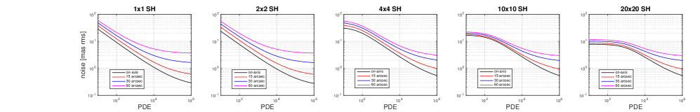
We have simulated tilt-removed random draws from the residual tomographic PSDs across the field simulated with Fast-F [12] for multiple wavelengths. We consider SH-WFS with 1, 2, 4, 10 and 20 sub-apertures (linear).

Figure 1 shows the noise curves fitted to the simulated ones for all the LO-WFS cases considered – with photon-noise only for the time being. These curves are in good agreement with standard expressions (in angle rms units)

$$\sigma_{\eta}=\frac{\theta_{b}}{\textsf{SNR}},[radrms]$$ (10)

where $\theta_{b}$ is the effective spot size of the sub-aperture and SNR is the signal-to-noise ratio of a single sub-aperture, when the field-dependent Strehl-ratio (SR) and PSF FWHM across the field are taken into account. However, these curves have a major advantage: non-linear effects like saturation at low flux levels and aliasing causing the roll-off at high-fluxes are taken into account. The behaviour far from these extremes is, as expected, $\propto n_{ph}^{-1/2}$

Figure 1: Noise curves comparing the model in this section to FAST-F computed noise levels as a function of the PDE (photon-detection equivalent) for full-pupil SH (1x1) to 20x20 SH operating in H-band. Saturation occurs on low-flux with increasing number of sub-apertures. Aliasing is seen on the high-end flux cases due to aliasing.

3 Isoplanatic tilt correction

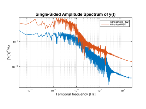
3.1 Isoplanatic input disturbances

We consider stationary and non-stationary sources of tilt. The former are depicted in Fig. 2 where the temporal PSD of both the turbulent tilt modes causing image jitter and wind-buffeting on the telescope structure cause image motion.

Figure 2: Power-spectral densities for the atmosphere-induced and wind-induced image jitter. The latter was simulated with wind face on aligned with the main axis are depicted (ESO internal report). For the meadian seeing conditions simulated (see below Fig. 9 for the Cn2 profiles) we get $\sim$ 20 mas rms and $\sim$270 mas rms input disturbances respectively.

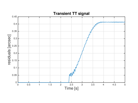
We further consider the non-stationary tilt from M1-3 off-loading to M4 causing a transient signal of about 400 mas rms roughly every 5 min (baseline) represented in Fig 3.

Figure 3: Transient signal affecting M4 every 5 minutes.

3.2 Handover scenarios

Isoplanatic tilt will be corrected at the telescope level by up to three off-axis tilt sensors guiding on faint stars not vignetting the instrument’s field.

We are currently evaluating two scenarios

1. sequential handover, where the instrument tilt signal alone drives M4/M5 after a transitioning period from the telescope over to the instrument

2. cascaded handover, where the off-axis tilt signals from the telescope and the on-axis (or closer in) instrument tilt are mingled to drive M4/M5

Although we do not cover the transitioning period in this work, we note the approach outlined in Raynaud et al [13]

3.3 Sequential handover

We consider four control strategies broadly cited in the literature [14, 15, 9]

1. double-stage composed of two single integrators and off-load loops

2. optimised gain double integrator with lead filter

3. LQG with i) AR1 and ii) AR2 temporal evolution models

The last three are coupled to a order-1 temporal filter with a 10 Hz cut-off frequency (subject to optimisation not done here although possible[14]) that low-pass filters tilt signals to M5 and assigns its complement to M4.

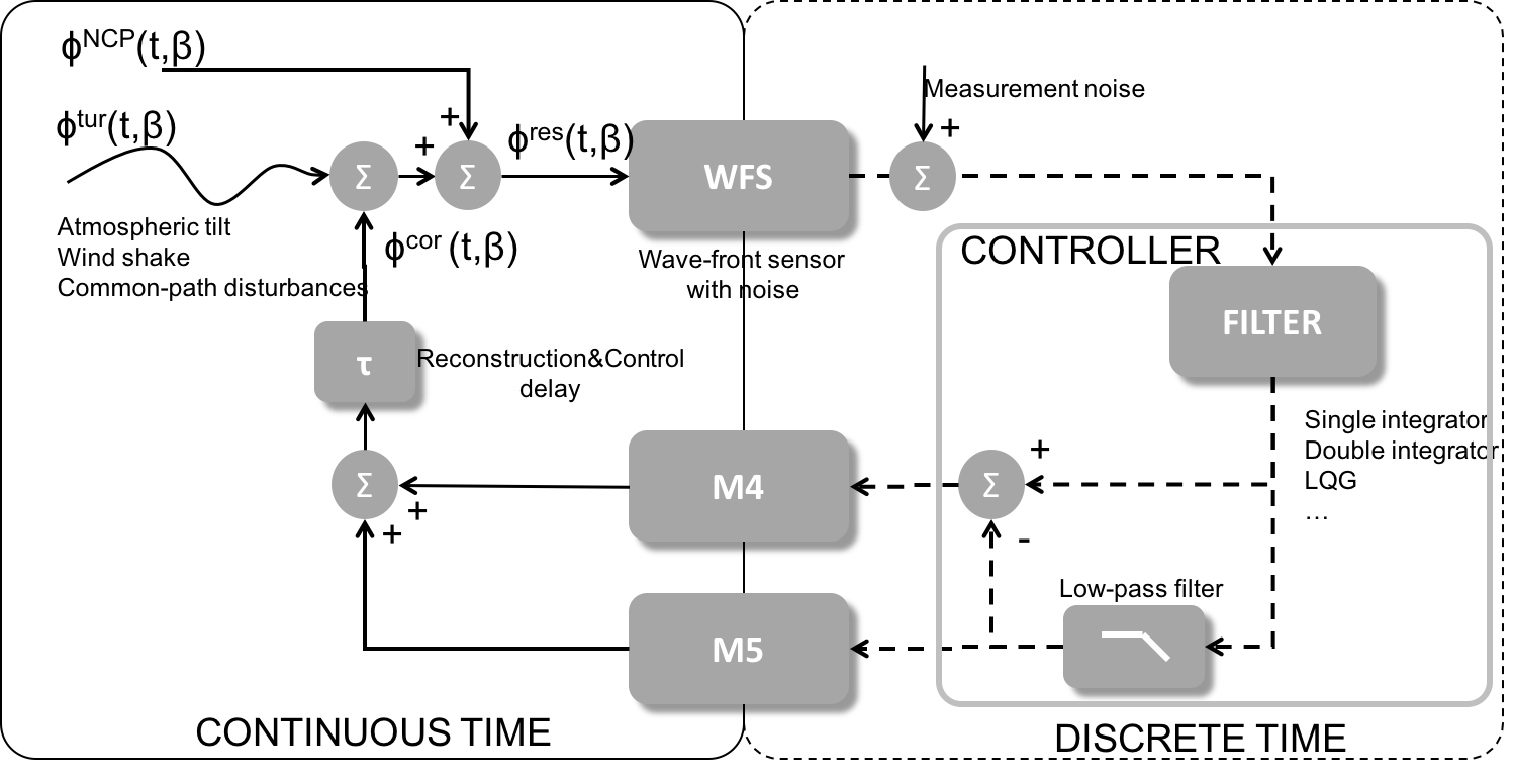
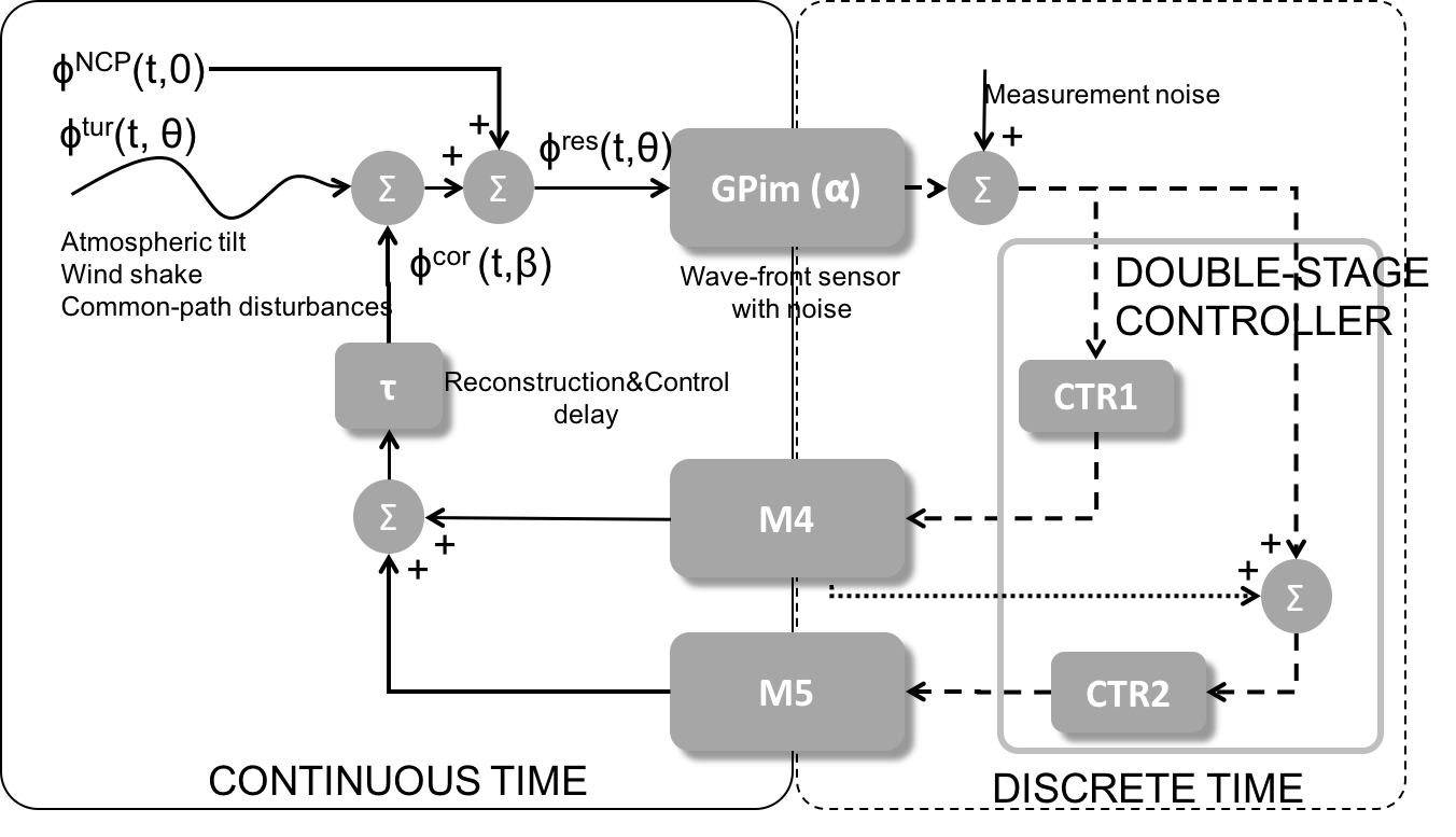
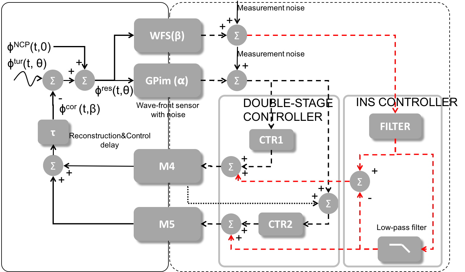
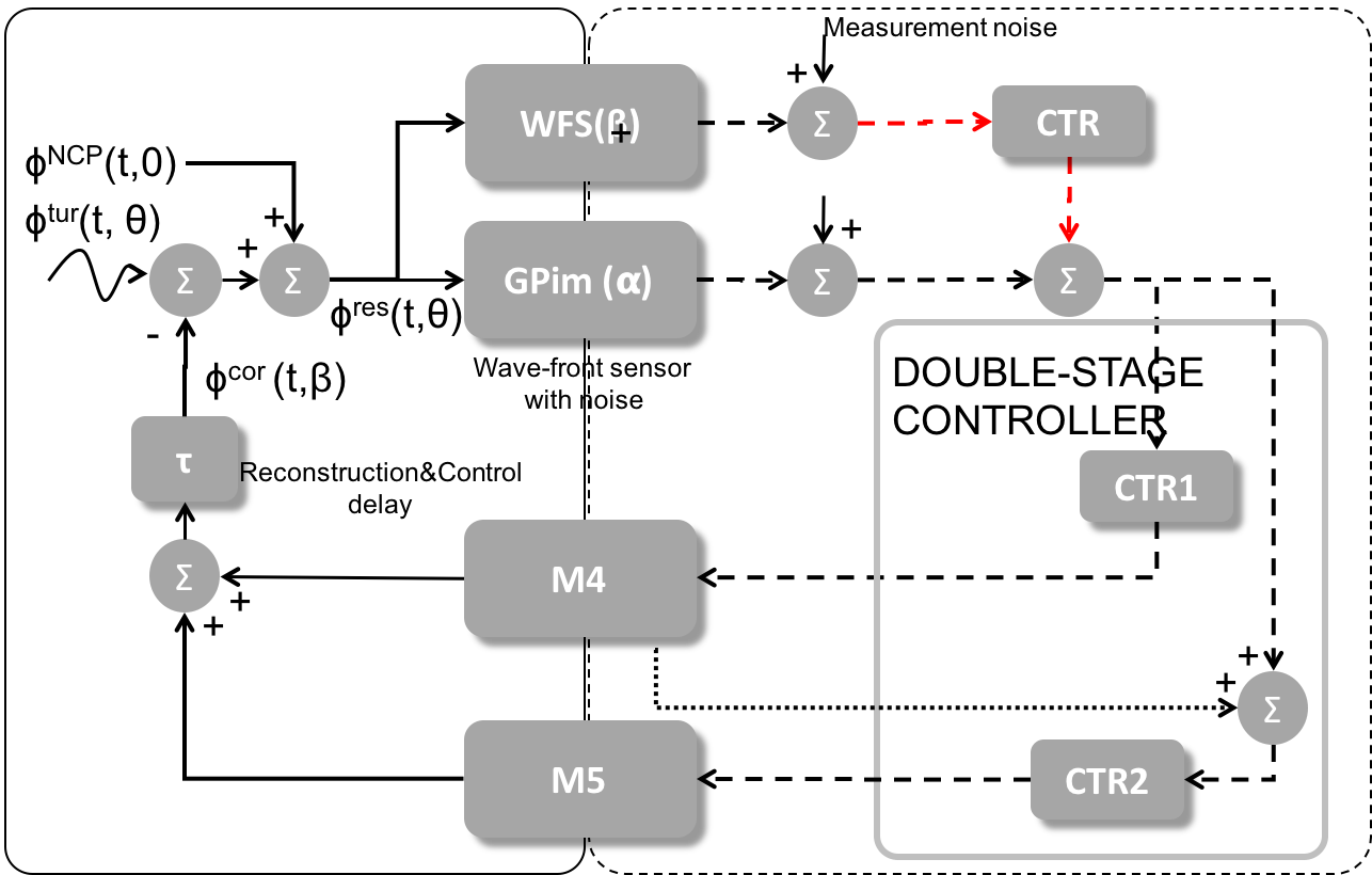
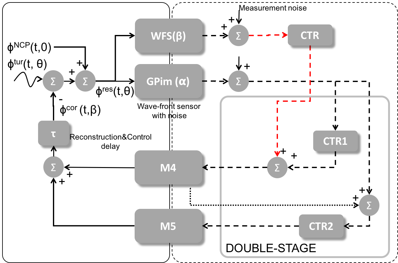
Figure 4 provides a block-diagram for integrator-based and LQG controllers.

Figure 4: General block diagram for TT control. The low-pass filter is subject to optimisation in terms of its cut-off frequency and model order.

For the double-stage controller, a different off-loading strategy is obtained with two single integrators as is shown in Fig. 5, but with an overall low-frequency rejection typical of a double-integrator i.e. 20dB/decade.

Figure 5: Double-stage block diagram for TT control where CRT1 and CRT2 are integrators of the kind $g/({1-e^{-T_{s}s}})$. The electric signal off from M4 consists in positioning sensors outputs.

3.3.1 Atmospheric and wind-induced tilt handling

The rejection transfer function is gathered as

$$H_{RTF}=\left|\frac{1}{1+h_{ol}}\right|^{2}$$ (11)

and

$$H_{NTF}=\left|\frac{h_{sys}}{1+h_{ol}}\right|^{2}$$ (12)

where $h_{sys}=h_{ol}/h_{wfs}$.

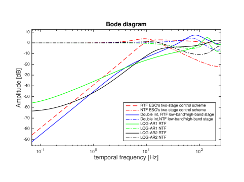
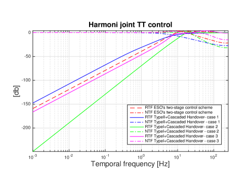
Figure 6 summarises the results thus far, depicting the rejection and noise transfer functions. In Table 1 numerical results are provided.

Figure 6: Controller’s rejection and noise transfer functions.

Table 1: Residuals in nm rms, noise propagation coefficients and stability margins.

Controller	Residual	Noise-propagation	gain margin	phase margin
	mas rms	coefficient
Double stage	2.6	0.17	16dB@73Hz	44.5o@13.1Hz
Double-integrator+lead	1.57	0.99	5.7dB@101Hz	42.7o@50.9Hz
LQG + AR1	1.81	0.46	7.5dB@145Hz	29.9o@64.4Hz
LQG + AR2	1.15	0.31	12dB@215Hz	149o@30.2Hz

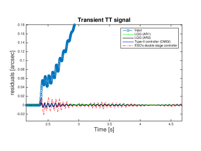
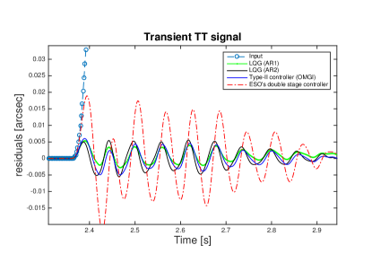
3.3.2 Transient handling

When dealing with non-stationary signals as the transient caused by off-loading M1-3-accumulated errors over to M4, transfer function analysis can no longer be applied. We thus run the transient through the controllers using time-domain simulations – Fig. 7. Note all the controllers but the double-stage keep the residual to within $\sim$6 mas whereas the latter, on account of its limited temporal bandwidth presents a spike of roughly 3 times as much, i.e. $\sim$18 mas.

Figure 7: Transient handling by the different controllers. The double-integrator+lead and the LQGs all keep the residual within $\pm$ 6 mas rms whereas the double-stage, on account of its limited closed-loop bandwidth achieves an intolerable 18 mas peak value.

3.3.3 Vibrations handling

Although we have processed various input signals with vibration peaks following [8] we defer to a later stage the full results when spectra from the E-ELT becomes available [7].

3.4 Cascaded handover

In cascaded handover, M4&M5 are driven jointly by the telescope and instrument’s tilt signals.

We foresee three options

1. LOWFS signals are processed and filtered with a custom-filter and dispatched directly to M4 and M5 following the low-pass/high-pass strategy presented above. The overall open-loop transfer function becomes

   $$h_{ol}=h_{WFS}h_{dac}h_{lag}\left\{\begin{array}[]{c}\left[\gamma h_{C4}+(1-\gamma)h_{CTR}(1-h_{low})\right]h_{m4}+\\ \left[-\gamma+\left[-\gamma h_{C4}+(1-\gamma)h_{CTR}(1-h_{low})\right]h_{m4}\right]h_{C5}h_{m5}+\\ (1-\gamma)h_{CTR}h_{low}h_{m5}\end{array}\right\}$$ (13)

   where $\gamma\in[0\cdots 1]$ is a user-defined parameter that balances the relative weight on the instrument LOWFS with respect to the telescope off-axis tilt signals

2. instrument tilt is added in series to telescope tilt and later filtered by the double-stage

   $$h_{ol}=h_{WFS}\left[-\gamma+(1-\gamma)h_{CTR}\right]h_{dac}h_{lag}\left(h_{C4}h_{m4}+h_{C5}h_{m5}+h_{C4}h_{m4}h_{C5}h_{m5}\right)$$ (14)

3. instrument tilt is affected solely to M4, the double stage taking charge of off-loading it to M5 as is goes

   $$h_{ol}=h_{WFS}h_{lag}\left[-\gamma+(1-\gamma)h_{CTR}\right]h_{dac}h_{lag}\left(h_{C4}h_{m4}+h_{C5}h_{m5}+h_{C4}h_{m4}h_{C5}h_{m5}\right)$$ (15)

conveniently depicted in Fig 8. A joint optimisation of $\gamma$ and the integrator gains (both for the two single integrators in the double-stage and the one for the instrument controller) has not been conducted. Results may therefore be different from the ones depicted in Fig 8; however in a cascaded handover the double-stage bandwidth will always limit the overall bandwidth of the controller.

Figure 8: (Top:) Three options tested for the cascaded handover scenario. (Bottom:) the corresponding rejection transfer functions when the instrument tilt controller is an optimised-gain double-integrator+lead-filter (blue-left, case 1), whereas cases 2 and 3 (respectively green and magenta) used a single optimised-gain integrator. All cases with $\gamma$ = 1/2. Red-dashed curves for the double-integrator in stand-alone mode for comparison.

4 Tilt anisoplanatism in laser-assisted AO tomography

The NGS modes in laser-tomography AO are defined as the null modes of the high-order LGS measurement space, i.e., modes that produce average slope $\neq$ 0, but that due to the LGS tilt indetermination, cannot be measured by the latter. In other words, the null space can be thought of as the combination of all the modes that have non-null projection onto the angle-of-arrival ( = not just Zernike tip and tilt but also higher order Zernike modes).

4.1 Tilt tomography

To estimate the tilt in the science direction of interest we consider the following options

1. Tilt tomography with spatio-angular reconstruction [2, 16]

   Since for LTAO only pupil-plane tilt is required (no fitting on multiple DMs) we use a simplified measurement model involving the pupil-plane turbulence only

   $${\mathbf{s}}_{\boldsymbol{\alpha}}(t)=\mathbf{G}{\boldsymbol{\psi}}_{\boldsymbol{\alpha}}(t)+{\boldsymbol{\eta}}(t)$$ (16)

   The minimum mean square error (MMSE) tilt estimate assuming ${\mathbf{s}}$ and ${\boldsymbol{\psi}}$ are zero-mean and jointly Gaussian is seamlessly found to be, for the $N_{\beta}$-science directions of interest [17]

   $$\mathcal{E}\{{\boldsymbol{\psi}}_{\boldsymbol{\beta}}|{\mathbf{s}}_{\boldsymbol{\alpha}}\}\triangleq\boldsymbol{\Sigma}_{({\boldsymbol{\psi}}_{\boldsymbol{\beta}},{\mathbf{s}}_{\boldsymbol{\alpha}})}\boldsymbol{\Sigma}^{-1}_{{\mathbf{s}}_{\boldsymbol{\alpha}}}{{\mathbf{s}}}_{\boldsymbol{\alpha}}=\widehat{{\boldsymbol{\psi}}}_{\boldsymbol{\beta}}$$ (17)

   where $\mathcal{E}\{X|Y\}$ stands for mathematical expectation of $X$ conditioned to $Y$. Since in general ${\boldsymbol{\beta}}\neq{\boldsymbol{\alpha}}$, Eq. (17) follows from $\mathcal{E}\{{\boldsymbol{\psi}}_{\boldsymbol{\beta}}|{\mathbf{s}}_{\boldsymbol{\alpha}}\}=\mathcal{E}\{{\boldsymbol{\psi}}_{\boldsymbol{\beta}}|\mathcal{E}\{{\boldsymbol{\psi}}_{\boldsymbol{\alpha}}|{\mathbf{s}}_{\boldsymbol{\alpha}}\}\}$. Matrices $\boldsymbol{\Sigma}_{({\boldsymbol{\psi}}_{\boldsymbol{\beta}},{\mathbf{s}}_{\boldsymbol{\alpha}})}$ and $\boldsymbol{\Sigma}_{{\mathbf{s}}_{\boldsymbol{\alpha}}}$ are spatio-angular covariance matrices that relate the tilt on direction ${\boldsymbol{\alpha}}$ to that on direction ${\boldsymbol{\beta}}$. These matrices are computed using formulae in [18] integrated in the simulator OOMAO [19], provided knowledge of the $C_{n}^{2}$ atmospheric profile is passed as input. Figure 9 depicts the 35-layer $C_{n}^{2}$ profile from ESO’s site testing campaigns with a seeing of $0.65^{\prime\prime}$ (for a $r_{0}=0.151\,m@0.5\mu m$) and $L_{0}=25\,m$.

   

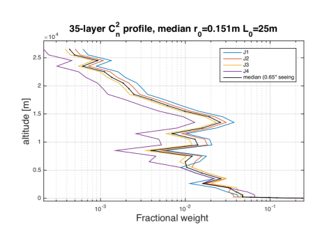
   Figure 9: 35-layer median $C_{n}^{2}$ profile;

   Under the spatio-angular approach, it is also possible to compute ${\boldsymbol{\psi}}(\boldsymbol{\rho},{\boldsymbol{\beta}},t+\Delta)$, i.e., temporally predict the TT ahead in time by adjusting the angles over which the correlations are computed [2].

   $$\mathbf{E}=\boldsymbol{\Sigma}_{({\boldsymbol{\psi}}_{\boldsymbol{\beta}},{\mathbf{s}}_{\boldsymbol{\alpha}})}\boldsymbol{\Sigma}^{-1}_{{\mathbf{s}}_{\boldsymbol{\alpha}}}{{\mathbf{s}}}_{\boldsymbol{\alpha}}$$ (18)

2. Isoplanatic tilt correction (GLAO-like) which consists in averaging the tilt measurements obtained across the field

   $$\mathbf{E}=\frac{1}{nGs}\sum_{i=1}^{nGs}\mathbf{G}^{\dagger}{{\mathbf{s}}}_{{\boldsymbol{\alpha}},i}$$ (19)

3. Tilt tomography using virtual DMs over two layers [1]

   $$\mathbf{E}=\mathbf{H}_{\boldsymbol{\beta}}\left(\mathbf{H}_{\boldsymbol{\alpha}}^{\mathsf{T}}\mathbf{G}^{\mathsf{T}}\boldsymbol{\Sigma}_{\eta}^{-1}\mathbf{G}\mathbf{H}_{\boldsymbol{\alpha}}\right)^{-1}\mathbf{H}_{\boldsymbol{\alpha}}^{\mathsf{T}}\mathbf{G}^{\mathsf{T}}\boldsymbol{\Sigma}_{\eta}^{-1}$$ (20)

   where we used the measurement model

   $${\mathbf{s}}_{\boldsymbol{\alpha}}(t)=\mathbf{G}\mathbf{H}_{\boldsymbol{\alpha}}{\boldsymbol{\varphi}}(t)+{\boldsymbol{\eta}}(t)$$ (21)

   where $\mathbf{G}$ is an aperture-plane phase-to-gradient matrix representing the SH-WFS and $\mathbf{H}$ a ray-tracing operator from atmospheric layers to the pupil-plane.

   This reconstructor is a noise-weighted reconstructor. In case of equally noisy measurements it boils down to the simple averaging (GLAO-like) case.

4.2 Tomographic error in open-loop

For the MMSE case, the standard performance assessment formulae apply.

Starting from

$$\sigma^{2}({\boldsymbol{\beta}})=\left\langle{\left\|{\boldsymbol{\psi}}({\boldsymbol{\beta}})-\widehat{{\boldsymbol{\psi}}}({\boldsymbol{\beta}})\right\|^{2}}\right\rangle$$ (22)

with $\widehat{{\boldsymbol{\psi}}}({\boldsymbol{\beta}})=\mathbf{R}{{\mathbf{s}}}({\boldsymbol{\alpha}})$ we get

$$\sigma^{2}({\boldsymbol{\beta}}) =\operatorname{trace}\{\boldsymbol{\Sigma}_{\boldsymbol{\beta}}\}+\operatorname{trace}\{\mathbf{R}\mathbf{G}\boldsymbol{\Sigma}_{\boldsymbol{\alpha}}\mathbf{G}^{\mathsf{T}}\mathbf{R}^{\mathsf{T}}\}$$ (23)

$$-\operatorname{trace}\{\mathbf{R}\mathbf{G}\boldsymbol{\Sigma}_{{\boldsymbol{\beta}},{\boldsymbol{\alpha}}}\}-\operatorname{trace}\{\boldsymbol{\Sigma}_{{\boldsymbol{\alpha}},{\boldsymbol{\beta}}}\mathbf{G}^{\mathsf{T}}\mathbf{R}^{\mathsf{T}}\}$$ (24)

$$+\operatorname{trace}\{\mathbf{R}\boldsymbol{\Sigma}_{\boldsymbol{\eta}}\mathbf{R}^{\mathsf{T}}\}$$ (25)

$$=\sigma^{2}_{aniso}+\sigma^{2}_{noise}$$ (26)

For stars of equal magnitude, the virtual DMs tomography boils down to the GLAO-like reconstructor as it is straightforward to show for diagonal noise covariance matrices of equal entries. Simulations have shown that in open loop the spatio-angular reconstructor is superior specially for large off-axis distances. In what follows we will always use it and leave a more complete comparison for later work.

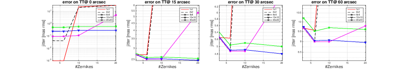
Figure 10 depicts the tomographic error as a function of the number of Zernike modes estimated from measurements out of LOWFS from 1x1 to 20x20 sub-apertures. As expected, for on-axis observations the least number of sub-apertures is preferred whereas for off-axis the optimum seems to be a 10x10 sub-aperture SHWFS with 20+ Zernike modes estimated. We understand this as a trade-off between the noise propagation (more sub-apertures means more noise) and the pure tomographic error (exploiting correlations of tilt with higher-order modes is beneficial).

Figure 10: Tomographic error as a function of the number of Zernike modes estimated from measurements

4.3 Error budget in closed-loop

We splat the the errors as tomographic, noise and temporal under the assumption that they are independent [20]

$$\sigma^{2}({\boldsymbol{\beta}})=\sigma^{2}_{aniso}+\sigma^{2}_{noise}+\sigma^{2}_{tempo}$$ (27)

where $\sigma^{2}_{aniso}$ is computed as in Eq. (22) and

$$\sigma^{2}_{noise}=\operatorname{trace}\{\mathbf{R}\boldsymbol{\Sigma}_{{\boldsymbol{\eta}}^{\prime}}\mathbf{R}^{\mathsf{T}}\}$$ (28)

with the horizontal elements of the loop-filtered noise covariance matrix populated with

$$\sigma^{2}_{{\boldsymbol{\eta}}^{\prime}}=2T_{s}\int_{0}^{1/2/T_{s}}NTF(\nu)\mathrm{d}\nu\,\,\,\sigma^{2}_{{\boldsymbol{\eta}}}$$ (29)

with $NTF(\nu)$ from Eq. (12). The temporal error

$$\sigma^{2}_{tempo}=\int_{0}^{1/2/T_{s}}RTF(\nu)PSD_{\varphi}(\nu)\mathrm{d}\nu$$ (30)

where $RTF(\nu)$ is gathered for different controller options from Eq. (11).

5 Assessing sky-coverage

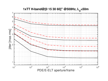
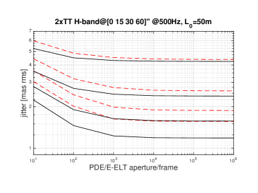
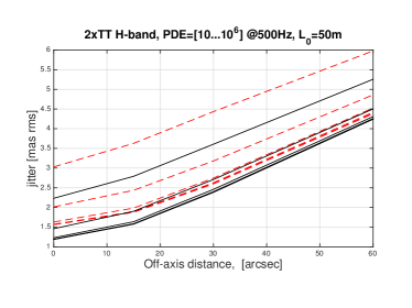
In this section we investigate the residual jitter as a function of the field and the photon flux. We have used the LQG+AR2 shown previously which provided the least isoplanatic tilt residual – see Table 1. Figure 11 shows the residual jitter with one or two TT measurements in the field (symmetric around the origin, same flux on both). We obtain a 1.2  mas rms jitter for $10^{6}$ PDE/aperture/$m^{2}$ on axis with 1 SH and only a small improvement with 2 SH.

On the opposite end, residual jitter of roughly 5.5 mas rms for 10 PDE/aperture/$m^{2}$ 1 arcmin off-axis which lowers to 5 mas rms in case 2 TT stars are used.

Figure 11: (Top-panel) Left: Residual jitter (ATM+wind-shake on 1 axis) as a function of the PDE/aperture/frame using a single-aperture SH-WFS probing a 35-layer ESO atmospheric profile with $L_{0}$= 50 m at angles [0, 15, 30, 60] arcsec. Red: optimised double integrator+lead filter, black: LQG. Left: same data plotted as a function of the off-axis-distance for different noise levels as a function of the PDE rangin from 10 to $10^{6}$. (Bottom-panel): same as top-panel with a second TT for secondary guiding.

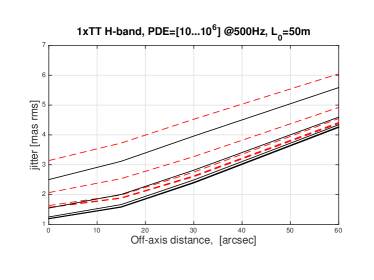
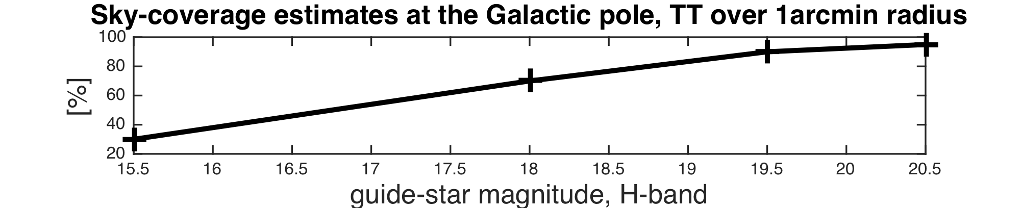
With these values we could compute sky-coverage estimates at the galactic pole considering a wide-band tilt measurement from I- to K-band in a field of 1 arcmin radius – as is shown in Fig. 12 as a function of the H-band magnitude[4].

Figure 12: Sky-coverage estimates at the galactic pole.

6 Outlook

Our simulations of isoplanatic tilt control for the Harmoni project show that LQG controllers in stand-alone mode (i.e. sequential handover) ensuring a 40db/dec at low-frequencies with 500Hz temporal frame-rate ensure the least residual whilst being stable even in the presence of non-stationary transients affecting the system every 5 minutes. Work on the cascaded handover mode where the instrument and telescope’s TT controllers work in tandem needs further parameter optimisation, although it seems to us a less promising path at this time.

Regarding tilt anisoplanatism we’ve found

• the use of secondary guiding improves the use of 1 single tilt measurement in the field only slightly (less than 10%)

• use of single-aperture SH for tilt measurement is best in the centre of the field whereas a 10x10 SH seems a better option when using a start farther off-axis up to 1 arcmin radius

• the spatio-angular tilt tomography controller ensures least residuals when compared to a GLAO-like reconstructor averaging the tilt in the field or to the virtual-DM reconstructor used in MCAO

Our preliminary sky-coverage estimates indicate 70% for H- magnitude guide-stars at the galactic pole over 1 arcmin radius.