Reanalysis of the $X(3915)$, $X(4500)$ and $X(4700)$ with QCD sum rules

Zhi-Gang Wang 111E-mail: zgwang@aliyun.com.

Department of Physics, North China Electric Power University, Baoding 071003, P. R. China

Abstract

In this article, we study the $C\gamma_{5}\otimes\gamma_{5}C$ type and $C\otimes C$ type scalar $cs\bar{c}\bar{s}$ tetraquark states with the QCD sum rules by calculating the contributions of the vacuum condensates up to dimension 10 in a consistent way. The ground state masses $M_{C\gamma_{5}\otimes\gamma_{5}C}=3.89\pm 0.05\,\rm{GeV}$ and $M_{C\otimes C}=5.48\pm 0.10\,\rm{GeV}$ support assigning the $X(3915)$ to be the ground state $C\gamma_{5}\otimes\gamma_{5}C$ type tetraquark state with $J^{PC}=0^{++}$, but do not support assigning the $X(4700)$ to be the ground state $C\otimes C$ type $cs\bar{c}\bar{s}$ tetraquark state with $J^{PC}=0^{++}$. Then we tentatively assign the $X(3915)$ and $X(4500)$ to be the 1S and 2S $C\gamma_{5}\otimes\gamma_{5}C$ type scalar $cs\bar{c}\bar{s}$ tetraquark states respectively, and obtain the 1S mass $M_{\rm 1S}=3.85^{+0.18}_{-0.17}\,\rm{GeV}$ and 2S mass $M_{\rm 2S}=4.35^{+0.10}_{-0.11}\,\rm{GeV}$ from the QCD sum rules, which support assigning the $X(3915)$ to be the 1S $C\gamma_{5}\otimes\gamma_{5}C$ type tetraquark state, but do not support assigning the $X(4500)$ to be the 2S $C\gamma_{5}\otimes\gamma_{5}C$ type tetraquark state.

PACS number: 12.39.Mk, 12.38.Lg

Key words: Tetraquark state, QCD sum rules

1 Introduction

Recently, the LHCb collaboration performed the first full amplitude analysis of the decays $B^{+}\to J/\psi\phi K^{+}$ with $J/\psi\to\mu^{+}\mu^{-}$, $\phi\to K^{+}K^{-}$ with a data sample of 3 fb-1 of $pp$ collision data collected at $\sqrt{s}=7$ and $8$ TeV with the LHCb detector, confirmed the two old particles $X(4140)$ and $X(4274)$ in the $J/\psi\phi$ mass spectrum with statistical significance $8.4\sigma$ and $6.0\sigma$, respectively, determined the quantum numbers to be $J^{PC}=1^{++}$ with statistical significance $5.7\sigma$ and $5.8\sigma$, respectively [1]. Moreover, the LHCb collaboration observed two new particles $X(4500)$ and $X(4700)$ in the $J/\psi\phi$ mass spectrum with statistical significance $6.1\sigma$ and $5.6\sigma$, respectively, determined the quantum numbers to be $J^{PC}=0^{++}$ with statistical significance $4.0\sigma$ and $4.5\sigma$, respectively [1]. The measured masses and widths are

$\displaystyle X(4140):M=4146.5\pm 4.5^{+4.6}_{-2.8}\mbox{ MeV}\,,\,\Gamma=83\pm 21^{+21}_{-14}\mbox{ MeV}\,,$
$\displaystyle X(4274):M=4273.3\pm 8.3^{+17.2}_{-3.6}\mbox{ MeV}\,,\,\Gamma=56\pm 11^{+8}_{-11}\mbox{ MeV}\,,$
$\displaystyle X(4500):M=4506\pm 11^{+12}_{-15}\mbox{ MeV}\,,\,\Gamma=92\pm 21^{+21}_{-20}\mbox{ MeV}\,,$
$\displaystyle X(4700):M=4704\pm 10^{+14}_{-24}\mbox{ MeV}\,,\,\Gamma=120\pm 31^{+42}_{-33}\mbox{ MeV}\,.$ (1)

There have been several possible assignments for the two new particles $X(4500)$ and $X(4700)$.

In Ref.[2], Chen et al study the newly observed $X(4500)$ and $X(4700)$ based on the diquark-antidiquark configuration within the framework of QCD sum rules, and interpret them as the D-wave $cs\bar{c}\bar{s}$ tetraquark states with $J^{P}=0^{+}$.

In Ref.[3], Liu studies the possible rescattering effects contribute to the process $B^{+}\to J/\psi\phi K^{+}$, and observes that the $D_{s}^{*+}D_{s}^{-}$ rescattering via the open-charmed meson loops and the $\psi^{\prime}\phi$ rescattering via the $\psi^{\prime}K_{1}$ loops may simulate the structures of the $X(4140)$ and $X(4700)$, respectively, and it is hard to attribute the $X(4274)$ and $X(4500)$ to the P-wave threshold rescattering effects.

In Ref.[4], Maiani, Polosa and Riquer assign the $X(4500)$ and $X(4700)$ to be the 2S tetraquark states based on the constituent diquark model. Also in Ref.[5], Zhu assigns the $X(4500)$ and $X(4700)$ to be the 2S tetraquark states based on the constituent diquark model.

In Ref.[6], Lebed and Polosa propose that the $X(3915)$ is the ground state $cs\bar{c}\bar{s}$ state based on lacking of the observed $D\bar{D}$ and $D^{*}\bar{D}^{*}$ decays, and attribute the single known decay mode $J/\psi\omega$ to the $\omega-\phi$ mixing effect.

The diquarks $\varepsilon^{ijk}q^{T}_{j}C\Gamma q^{\prime}_{k}$ in color antitriplet have five structures in Dirac spinor space, where $C\Gamma=C\gamma_{5}$, $C$, $C\gamma_{\mu}\gamma_{5}$, $C\gamma_{\mu}$ and $C\sigma_{\mu\nu}$ for the scalar, pseudoscalar, vector, axialvector and tensor diquarks, respectively. In Ref.[7], we study the masses and pole residues of the $X(3915)$, $X(4500)$ and $X(4700)$ in the scenario of tetraquark states with the QCD sum rules by calculating the contributions of the vacuum condensates up to dimension 10. The theoretical calculations support assigning the $X(3915)$ and $X(4500)$ to be the 1S and 2S $C\gamma_{\mu}\otimes\gamma^{\mu}C$ type scalar $cs\bar{c}\bar{s}$ tetraquark states, respectively, and assigning the $X(4700)$ to be the 1S $C\gamma_{\mu}\gamma_{5}\otimes\gamma_{5}\gamma^{\mu}C$ type scalar $cs\bar{c}\bar{s}$ tetraquark state. In subsequent work, we take the $X(4140)$ as the diquark-antidiquark type $cs\bar{c}\bar{s}$ tetraquark state with $J^{PC}=1^{++}$, and study the mass and pole residue with the QCD sum rules in details by constructing two types interpolating currents. The numerical results $M_{X_{L,+}}=3.95\pm 0.09\,\rm{GeV}$ and $M_{X_{H,+}}=5.00\pm 0.10\,\rm{GeV}$ disfavor assigning the $X(4140)$ to be the $C\gamma_{5}\otimes\gamma_{\mu}C+C\gamma_{\mu}\otimes\gamma_{5}C$ type or $C\otimes\gamma_{5}\gamma_{\mu}C+C\gamma_{\mu}\gamma_{5}\otimes C$ type tetraquark state with $J^{PC}=1^{++}$ [8].

The attractive interactions of one-gluon exchange favor formation of the diquarks in color antitriplet $\overline{3}_{c}$, flavor antitriplet $\overline{3}_{f}$ and spin singlet $1_{s}$ or flavor sextet $6_{f}$ and spin triplet $3_{s}$ [9]. The calculations based on the QCD sum rules also indicate that the favored configurations are the $C\gamma_{5}$ and $C\gamma_{\mu}$ diquark states [10, 11], and the heavy-light $C\gamma_{5}$ and $C\gamma_{\mu}$ diquark states have almost degenerate masses [10]. In Ref.[12], we construct the $C\gamma_{5}\otimes\gamma_{5}C$, $C\gamma_{\mu}\otimes\gamma^{\mu}C$, $C\gamma_{\mu}\gamma_{5}\otimes\gamma_{5}\gamma^{\mu}C$ type interpolating currents to study the scalar tetraquark states with the QCD sum rules in a systematic way, and observe that the $C\gamma_{5}\otimes\gamma_{5}C$ type and $C\gamma_{\mu}\otimes\gamma^{\mu}C$ type scalar $cs\bar{c}\bar{s}$ tetraquark states have almost degenerate masses, about $4.44\,\rm{GeV}$.

The value $4.44\,\rm{GeV}$ is not robust as the masses are extracted from the QCD spectral densities at the energy scale $\mu=1\,\rm{GeV}$. In Refs.[13, 14, 15], we explore the energy scale dependence of the masses $M_{X/Y/Z}$ of the hidden charm (bottom) tetraquark states in details for the first time, and suggest a formula,

$\displaystyle\mu$ $\displaystyle=$ $\displaystyle\sqrt{M^{2}_{X/Y/Z}-(2{\mathbb{M}}_{Q})^{2}}\,,$ (2)

with the effective heavy quark mass ${\mathbb{M}}_{Q}$ to determine the energy scales of the QCD spectral densities in the QCD sum rules, which works well.

Now we take a short digression to discuss the energy scale dependence of the QCD sum rules for the hidden charm or hidden bottom tetraquark states. The correlation functions $\Pi(p)$ can be written as

$\displaystyle\Pi(p)$ $\displaystyle=$ ∫4​mQ2​(ΞΌ)s0𝑑s​ρQ​C​D​(s,ΞΌ)sβˆ’p2+∫s0βˆžπ‘‘s​ρQ​C​D​(s,ΞΌ)sβˆ’p2,superscriptsubscript4subscriptsuperscriptπ‘š2π‘„πœ‡subscript𝑠0differential-d𝑠subscriptπœŒπ‘„πΆπ·π‘ πœ‡π‘ superscript𝑝2superscriptsubscriptsubscript𝑠0differential-d𝑠subscriptπœŒπ‘„πΆπ·π‘ πœ‡π‘ superscript𝑝2\displaystyle\int_{4m^{2}_{Q}(\mu)}^{s_{0}}ds\frac{\rho_{QCD}(s,\mu)}{s-p^{2}}+\int_{s_{0}}^{\infty}ds\frac{\rho_{QCD}(s,\mu)}{s-p^{2}}\,, (3)

through dispersion relation at the QCD side, where the $s_{0}$ are continuum threshold parameters. The $\Pi(p)$ are energy scale independent,

dd​μ​Π​(p)π‘‘π‘‘πœ‡Ξ π‘\displaystyle\frac{d}{d\mu}\Pi(p) $\displaystyle=$ $\displaystyle 0\,,$ (4)

which does not mean

ddβ€‹ΞΌβ€‹βˆ«4​mQ2​(ΞΌ)s0𝑑s​ρQ​C​D​(s,ΞΌ)sβˆ’p2β†’0,β†’π‘‘π‘‘πœ‡superscriptsubscript4subscriptsuperscriptπ‘š2π‘„πœ‡subscript𝑠0differential-d𝑠subscriptπœŒπ‘„πΆπ·π‘ πœ‡π‘ superscript𝑝20\displaystyle\frac{d}{d\mu}\int_{4m^{2}_{Q}(\mu)}^{s_{0}}ds\frac{\rho_{QCD}(s,\mu)}{s-p^{2}}\rightarrow 0\,, (5)

due to the following two reasons inherited from the QCD sum rules:
$\bullet$ Perturbative corrections are neglected, the higher dimensional vacuum condensates are factorized into lower dimensional ones therefore the energy scale dependence of the higher dimensional vacuum condensates is modified;
$\bullet$ Truncations $s_{0}$ set in, the correlation between the threshold $4m^{2}_{Q}(\mu)$ and continuum threshold $s_{0}$ is unknown.

In the QCD sum rules for the hidden charm or hidden bottom tetraquark states, the integrals

∫4​mQ2​(ΞΌ)s0𝑑s​ρQ​C​D​(s,ΞΌ)​exp⁑(βˆ’sT2),superscriptsubscript4subscriptsuperscriptπ‘š2π‘„πœ‡subscript𝑠0differential-d𝑠subscriptπœŒπ‘„πΆπ·π‘ πœ‡π‘ superscript𝑇2\displaystyle\int_{4m^{2}_{Q}(\mu)}^{s_{0}}ds\,\rho_{QCD}(s,\mu)\,\exp\left(-\frac{s}{T^{2}}\right)\,, (6)

are sensitive to the heavy quark masses $m_{Q}(\mu)$ or the energy scales $\mu$, where the $T^{2}$ denotes the Borel parameters. Variations of the heavy quark masses or the energy scales $\mu$ lead to changes of integral ranges $4m_{Q}^{2}(\mu)-s_{0}$ of the variable $ds$ besides the QCD spectral densities ρQ​C​D​(s,ΞΌ)subscriptπœŒπ‘„πΆπ·π‘ πœ‡\rho_{QCD}(s,\mu), therefore changes of the Borel windows and predicted masses and pole residues. We cannot obtain energy scale independent QCD sum rules, but we have an energy scale formula to determine the energy scales consistently.

According to the formula, the energy scale $\mu=1\,\rm{GeV}$ is too low to result in robust predictions [12]. In Ref.[7], we use the energy scale formula in Eq.(2) to determine the energy scales of the QCD spectral densities in the QCD sum rules, and observe that the $X(3915)$ and $X(4500)$ can be assigned to be the 1S and 2S $C\gamma_{\mu}\otimes\gamma^{\mu}C$ type scalar $cs\bar{c}\bar{s}$ tetraquark states, respectively, and the $X(4700)$ can be assigned to be the 1S $C\gamma_{\mu}\gamma_{5}\otimes\gamma_{5}\gamma^{\mu}C$ type scalar $cs\bar{c}\bar{s}$ tetraquark state. In Ref.[7], we obtain the values $M_{X(3915)}=3.91^{+0.21}_{-0.17}\,\rm{GeV}$, $M_{X(4500)}=4.50^{+0.08}_{-0.09}\,\rm{GeV}$ and $M_{X(4700)}=4.70^{+0.08}_{-0.09}\,\rm{GeV}$. The value $M_{X(3915)}=3.91^{+0.21}_{-0.17}\,\rm{GeV}$ is much smaller than the value $4.44\,\rm{GeV}$ obtained in Ref.[12]. If the $C\gamma_{5}\otimes\gamma_{5}C$ type and $C\gamma_{\mu}\otimes\gamma^{\mu}C$ type tetraquark states have degenerate masses, then the $X(3915)$ and $X(4500)$ can have another diquark-antidiquark structure, $C\gamma_{5}\otimes\gamma_{5}C$.

In this article, we study the $C\gamma_{5}\otimes\gamma_{5}C$ type and $C\otimes C$ type scalar $cs\bar{c}\bar{s}$ tetraquark states with the QCD sum rules by calculating the contributions of the vacuum condensates up to dimension 10 in a consistent way. In calculations, we use the energy scale formula to determine the optimal energy scales of the QCD spectral densities to extract to tetraquark masses to identify the $X(3915)$, $X(4500)$ and $X(4700)$.

The article is arranged as follows: we derive the QCD sum rules for the masses and pole residues of the 1S $C\gamma_{5}\otimes\gamma_{5}C$ type and $C\otimes C$ type $cs\bar{c}\bar{s}$ tetraquark states in section 2; in section 3, we derive the QCD sum rules for the masses and pole residues of the 1S and 2S $C\gamma_{5}\otimes\gamma_{5}C$ type $cs\bar{c}\bar{s}$ tetraquark states; section 4 is reserved for our conclusion.

2 QCD sum rules for the scalar tetraquark states $X_{L}$ and $X_{H}$

In the following, we write down the two-point correlation functions Ξ L/H​(p)subscriptΠ𝐿𝐻𝑝\Pi_{L/H}(p) in the QCD sum rules,

Ξ L/H​(p)subscriptΠ𝐿𝐻𝑝\displaystyle\Pi_{L/H}(p) $\displaystyle=$ $\displaystyle i\int d^{4}xe^{ip\cdot x}\langle 0|T\left\{J_{L/H}(x)J_{L/H}^{\dagger}(0)\right\}|0\rangle\,,$ (7)

where

$\displaystyle J_{L}(x)$ $\displaystyle=$ Ο΅i​j​k​ϡi​m​n​sj​(x)​C​γ5​ck​(x)​sΒ―m​(x)​γ5​C​cΒ―n​(x),superscriptitalic-Ο΅π‘–π‘—π‘˜superscriptitalic-Ο΅π‘–π‘šπ‘›superscript𝑠𝑗π‘₯𝐢subscript𝛾5superscriptπ‘π‘˜π‘₯superscriptΒ―π‘ π‘šπ‘₯subscript𝛾5𝐢superscript¯𝑐𝑛π‘₯\displaystyle\epsilon^{ijk}\epsilon^{imn}s^{j}(x)C\gamma_{5}c^{k}(x)\bar{s}^{m}(x)\gamma_{5}C\bar{c}^{n}(x)\,,
$\displaystyle J_{H}(x)$ $\displaystyle=$ Ο΅i​j​k​ϡi​m​n​sj​(x)​C​ck​(x)​sΒ―m​(x)​C​cΒ―n​(x),superscriptitalic-Ο΅π‘–π‘—π‘˜superscriptitalic-Ο΅π‘–π‘šπ‘›superscript𝑠𝑗π‘₯𝐢superscriptπ‘π‘˜π‘₯superscriptΒ―π‘ π‘šπ‘₯𝐢superscript¯𝑐𝑛π‘₯\displaystyle\epsilon^{ijk}\epsilon^{imn}s^{j}(x)Cc^{k}(x)\bar{s}^{m}(x)C\bar{c}^{n}(x)\,, (8)

where the $i$, $j$, $k$, $m$, $n$ are color indexes, the $C$ is the charge conjugation matrix. The scalar diquark states are more stable than the pseudoscalar diquark states, so we expect that the $C\gamma_{5}\otimes\gamma_{5}C$ type tetraquark states have much smaller masses than the corresponding $C\otimes C$ type tetraquark states, and add the subscripts $L$ and $H$ to denote the light and heavy tetraquark states, respectively.

At the phenomenological side, we can insert a complete set of intermediate hadronic states with the same quantum numbers as the current operators $J_{L/H}(x)$ into the correlation functions Ξ L/H​(p)subscriptΠ𝐿𝐻𝑝\Pi_{L/H}(p) to obtain the hadronic representation [16, 17]. After isolating the ground state contributions of the scalar $cs\bar{c}\bar{s}$ tetraquark states $X_{L/H}$, we get the results,

Ξ L​(p)subscriptΠ𝐿𝑝\displaystyle\Pi_{L}(p) $\displaystyle=$ $\displaystyle\frac{\lambda_{X_{L}}^{2}}{M_{X_{L}}^{2}-p^{2}}+\cdots\,\,,$
Ξ H​(p)subscriptΠ𝐻𝑝\displaystyle\Pi_{H}(p) $\displaystyle=$ $\displaystyle\frac{\lambda_{X_{H}}^{2}}{M_{X_{H}}^{2}-p^{2}}+\cdots\,\,,$ (9)

where the pole residues $\lambda_{X_{L/H}}$ are defined by $\langle 0|J_{L/H}(0)|X_{L/H}(p)\rangle=\lambda_{X_{L/H}}$.

In the following, we briefly outline the operator product expansion for the correlation functions Ξ L/H​(p)subscriptΠ𝐿𝐻𝑝\Pi_{L/H}(p) in perturbative QCD. We contract the $s$ and $c$ quark fields in the correlation functions Ξ L/H​(p)subscriptΠ𝐿𝐻𝑝\Pi_{L/H}(p) with Wick theorem, and obtain the results:

Ξ L​(p)subscriptΠ𝐿𝑝\displaystyle\Pi_{L}(p) $\displaystyle=$ $\displaystyle i\epsilon^{ijk}\epsilon^{imn}\epsilon^{i^{\prime}j^{\prime}k^{\prime}}\epsilon^{i^{\prime}m^{\prime}n^{\prime}}\int d^{4}xe^{ip\cdot x}$
$\displaystyle{\rm Tr}\left[\gamma_{5}C^{kk^{\prime}}(x)\gamma_{5}CS^{jj^{\prime}T}(x)C\right]{\rm Tr}\left[\gamma_{5}C^{n^{\prime}n}(-x)\gamma_{5}CS^{m^{\prime}mT}(-x)C\right]\,,$
Ξ H​(p)subscriptΠ𝐻𝑝\displaystyle\Pi_{H}(p) $\displaystyle=$ $\displaystyle i\epsilon^{ijk}\epsilon^{imn}\epsilon^{i^{\prime}j^{\prime}k^{\prime}}\epsilon^{i^{\prime}m^{\prime}n^{\prime}}\int d^{4}xe^{ip\cdot x}$ (10)
$\displaystyle{\rm Tr}\left[C^{kk^{\prime}}(x)CS^{jj^{\prime}T}(x)C\right]{\rm Tr}\left[C^{n^{\prime}n}(-x)CS^{m^{\prime}mT}(-x)C\right]\,,$

where the $S_{ij}(x)$ and $C_{ij}(x)$ are the full $s$ and $c$ quark propagators, respectively [17, 18],

$\displaystyle S^{ij}(x)$ $\displaystyle=$ i​δi​j​​x2​π2​x4βˆ’Ξ΄i​j​ms4​π2​x2βˆ’Ξ΄i​jβ€‹βŸ¨s¯​s⟩12+i​δi​j​​x​msβ€‹βŸ¨s¯​s⟩48βˆ’Ξ΄i​j​x2β€‹βŸ¨s¯​gs​σ​G​s⟩192+i​δi​j​x2​​x​msβ€‹βŸ¨s¯​gs​σ​G​s⟩1152𝑖subscript𝛿𝑖𝑗π‘₯2superscriptπœ‹2superscriptπ‘₯4subscript𝛿𝑖𝑗subscriptπ‘šπ‘ 4superscriptπœ‹2superscriptπ‘₯2subscript𝛿𝑖𝑗delimited-βŸ¨βŸ©Β―π‘ π‘ 12𝑖subscript𝛿𝑖𝑗π‘₯subscriptπ‘šπ‘ delimited-βŸ¨βŸ©Β―π‘ π‘ 48subscript𝛿𝑖𝑗superscriptπ‘₯2delimited-βŸ¨βŸ©Β―π‘ subscriptπ‘”π‘ πœŽπΊπ‘ 192𝑖subscript𝛿𝑖𝑗superscriptπ‘₯2π‘₯subscriptπ‘šπ‘ delimited-βŸ¨βŸ©Β―π‘ subscriptπ‘”π‘ πœŽπΊπ‘ 1152\displaystyle\frac{i\delta_{ij}\!\not\!{x}}{2\pi^{2}x^{4}}-\frac{\delta_{ij}m_{s}}{4\pi^{2}x^{2}}-\frac{\delta_{ij}\langle\bar{s}s\rangle}{12}+\frac{i\delta_{ij}\!\not\!{x}m_{s}\langle\bar{s}s\rangle}{48}-\frac{\delta_{ij}x^{2}\langle\bar{s}g_{s}\sigma Gs\rangle}{192}+\frac{i\delta_{ij}x^{2}\!\not\!{x}m_{s}\langle\bar{s}g_{s}\sigma Gs\rangle}{1152} (11)
βˆ’i​gs​Gα​βa​ti​ja​(​x​σα​β+σα​β​​x)32​π2​x2βˆ’i​δi​j​x2​​x​gs2β€‹βŸ¨s¯​s⟩27776βˆ’Ξ΄i​j​x4β€‹βŸ¨s¯​sβŸ©β€‹βŸ¨gs2​G​G⟩27648βˆ’18β€‹βŸ¨sΒ―j​σμ​ν​siβŸ©β€‹ΟƒΞΌβ€‹Ξ½π‘–subscript𝑔𝑠subscriptsuperscriptπΊπ‘Žπ›Όπ›½subscriptsuperscriptπ‘‘π‘Žπ‘–π‘—π‘₯superscriptπœŽπ›Όπ›½superscriptπœŽπ›Όπ›½π‘₯32superscriptπœ‹2superscriptπ‘₯2𝑖subscript𝛿𝑖𝑗superscriptπ‘₯2π‘₯superscriptsubscript𝑔𝑠2superscriptdelimited-βŸ¨βŸ©Β―π‘ π‘ 27776subscript𝛿𝑖𝑗superscriptπ‘₯4delimited-βŸ¨βŸ©Β―π‘ π‘ delimited-⟨⟩superscriptsubscript𝑔𝑠2𝐺𝐺2764818delimited-⟨⟩subscript¯𝑠𝑗superscriptπœŽπœ‡πœˆsubscript𝑠𝑖subscriptπœŽπœ‡πœˆ\displaystyle-\frac{ig_{s}G^{a}_{\alpha\beta}t^{a}_{ij}(\!\not\!{x}\sigma^{\alpha\beta}+\sigma^{\alpha\beta}\!\not\!{x})}{32\pi^{2}x^{2}}-\frac{i\delta_{ij}x^{2}\!\not\!{x}g_{s}^{2}\langle\bar{s}s\rangle^{2}}{7776}-\frac{\delta_{ij}x^{4}\langle\bar{s}s\rangle\langle g_{s}^{2}GG\rangle}{27648}-\frac{1}{8}\langle\bar{s}_{j}\sigma^{\mu\nu}s_{i}\rangle\sigma_{\mu\nu}
$\displaystyle-\frac{1}{4}\langle\bar{s}_{j}\gamma^{\mu}s_{i}\rangle\gamma_{\mu}+\cdots\,,$
$\displaystyle C_{ij}(x)$ $\displaystyle=$ $\displaystyle\frac{i}{(2\pi)^{4}}\int d^{4}ke^{-ik\cdot x}\left\{\frac{\delta_{ij}}{\!\not\!{k}-m_{c}}-\frac{g_{s}G^{n}_{\alpha\beta}t^{n}_{ij}}{4}\frac{\sigma^{\alpha\beta}(\!\not\!{k}+m_{c})+(\!\not\!{k}+m_{c})\sigma^{\alpha\beta}}{(k^{2}-m_{c}^{2})^{2}}\right.$
$\displaystyle\left.+\frac{g_{s}D_{\alpha}G^{n}_{\beta\lambda}t^{n}_{ij}(f^{\lambda\beta\alpha}+f^{\lambda\alpha\beta})}{3(k^{2}-m_{c}^{2})^{4}}-\frac{g_{s}^{2}(t^{a}t^{b})_{ij}G^{a}_{\alpha\beta}G^{b}_{\mu\nu}(f^{\alpha\beta\mu\nu}+f^{\alpha\mu\beta\nu}+f^{\alpha\mu\nu\beta})}{4(k^{2}-m_{c}^{2})^{5}}+\cdots\right\}\,,$
$\displaystyle f^{\lambda\alpha\beta}$ $\displaystyle=$ $\displaystyle(\!\not\!{k}+m_{c})\gamma^{\lambda}(\!\not\!{k}+m_{c})\gamma^{\alpha}(\!\not\!{k}+m_{c})\gamma^{\beta}(\!\not\!{k}+m_{c})\,,$
$\displaystyle f^{\alpha\beta\mu\nu}$ $\displaystyle=$ $\displaystyle(\!\not\!{k}+m_{c})\gamma^{\alpha}(\!\not\!{k}+m_{c})\gamma^{\beta}(\!\not\!{k}+m_{c})\gamma^{\mu}(\!\not\!{k}+m_{c})\gamma^{\nu}(\!\not\!{k}+m_{c})\,,$ (13)

and $t^{n}=\frac{\lambda^{n}}{2}$, the $\lambda^{n}$ is the Gell-Mann matrix, $D_{\alpha}=\partial_{\alpha}-ig_{s}G^{n}_{\alpha}t^{n}$ [17]. Then we compute the integrals both in coordinate space and in momentum space, and obtain the correlation functions Ξ L/H​(p)subscriptΠ𝐿𝐻𝑝\Pi_{L/H}(p), therefore the QCD spectral densities through dispersion relation. In this article, we take into account the vacuum condensates which are vacuum expectations of the operators of the orders π’ͺ​(Ξ±sk)π’ͺsuperscriptsubscriptπ›Όπ‘ π‘˜\mathcal{O}(\alpha_{s}^{k}) with $k\leq 1$ consistently. For the technical details, one can consult Ref.[19]. We neglect the radiative $\mathcal{O}(\alpha_{s})$ corrections for the perturbative contributions, it is a challenging or formidable work to calculate the radiative $\mathcal{O}(\alpha_{s})$ corrections in the QCD sum rules for hidden charm or hidden bottom tetraquark states, though the corrections may be large in the presence of two heavy quarks, just like in the QCD sum rules for the vector and axialvector $B_{c}$ mesons [20].

Once the analytical QCD spectral densities are obtained, we take the quark-hadron duality below the continuum thresholds $s^{0}_{L/H}$ and perform Borel transform with respect to the variable $P^{2}=-p^{2}$ to obtain the QCD sum rules:

Ξ»XL2​exp⁑(βˆ’MXL2T2)=∫4​mc2sL0𝑑s​ρL​(s)​exp⁑(βˆ’sT2),subscriptsuperscriptπœ†2subscript𝑋𝐿subscriptsuperscript𝑀2subscript𝑋𝐿superscript𝑇2superscriptsubscript4superscriptsubscriptπ‘šπ‘2superscriptsubscript𝑠𝐿0differential-d𝑠subscriptπœŒπΏπ‘ π‘ superscript𝑇2\displaystyle\lambda^{2}_{X_{L}}\,\exp\left(-\frac{M^{2}_{X_{L}}}{T^{2}}\right)=\int_{4m_{c}^{2}}^{s_{L}^{0}}ds\,\rho_{L}(s)\,\exp\left(-\frac{s}{T^{2}}\right)\,, (14)
Ξ»XH2​exp⁑(βˆ’MXH2T2)=∫4​mc2sH0𝑑s​ρH​(s)​exp⁑(βˆ’sT2),subscriptsuperscriptπœ†2subscript𝑋𝐻subscriptsuperscript𝑀2subscript𝑋𝐻superscript𝑇2superscriptsubscript4superscriptsubscriptπ‘šπ‘2superscriptsubscript𝑠𝐻0differential-d𝑠subscriptπœŒπ»π‘ π‘ superscript𝑇2\displaystyle\lambda^{2}_{X_{H}}\,\exp\left(-\frac{M^{2}_{X_{H}}}{T^{2}}\right)=\int_{4m_{c}^{2}}^{s_{H}^{0}}ds\,\rho_{H}(s)\,\exp\left(-\frac{s}{T^{2}}\right)\,, (15)

where

ρL​(s)subscriptπœŒπΏπ‘ \displaystyle\rho_{L}(s) $\displaystyle=$ $\displaystyle\rho_{0}(s)+\rho_{3}(s)+\rho_{4}(s)+\rho_{5}(s)+\rho_{6}(s)+\rho_{7}(s)+\rho_{8}(s)+\rho_{10}(s)\,,$
ρH​(s)subscriptπœŒπ»π‘ \displaystyle\rho_{H}(s) $\displaystyle=$ ρL​(s)|mcβ†’βˆ’mc,evaluated-atsubscriptπœŒπΏπ‘ β†’subscriptπ‘šπ‘subscriptπ‘šπ‘\displaystyle\rho_{L}(s)|_{m_{c}\to-m_{c}}\,, (16)
$\displaystyle\rho_{0}(s)$ $\displaystyle=$ $\displaystyle\frac{1}{512\pi^{6}}\int_{y_{i}}^{y_{f}}dy\int_{z_{i}}^{1-y}dz\,yz\,(1-y-z)^{3}\left(s-\overline{m}_{c}^{2}\right)^{2}\left(7s^{2}-6s\overline{m}_{c}^{2}+\overline{m}_{c}^{4}\right)$ (17)
+ms​mc256​π6β€‹βˆ«yiyf𝑑yβ€‹βˆ«zi1βˆ’y𝑑z​(y+z)​(1βˆ’yβˆ’z)2​(sβˆ’mΒ―c2)2​(5​sβˆ’2​mΒ―c2),subscriptπ‘šπ‘ subscriptπ‘šπ‘256superscriptπœ‹6superscriptsubscriptsubscript𝑦𝑖subscript𝑦𝑓differential-d𝑦superscriptsubscriptsubscript𝑧𝑖1𝑦differential-d𝑧𝑦𝑧superscript1𝑦𝑧2superscript𝑠superscriptsubscriptΒ―π‘šπ‘225𝑠2superscriptsubscriptΒ―π‘šπ‘2\displaystyle+\frac{m_{s}m_{c}}{256\pi^{6}}\int_{y_{i}}^{y_{f}}dy\int_{z_{i}}^{1-y}dz\,(y+z)\,(1-y-z)^{2}\left(s-\overline{m}_{c}^{2}\right)^{2}\left(5s-2\overline{m}_{c}^{2}\right)\,,
$\displaystyle\rho_{3}(s)$ $\displaystyle=$ βˆ’mcβ€‹βŸ¨s¯​s⟩16​π4β€‹βˆ«yiyf𝑑yβ€‹βˆ«zi1βˆ’y𝑑z​(y+z)​(1βˆ’yβˆ’z)​(sβˆ’mΒ―c2)​(2​sβˆ’mΒ―c2)subscriptπ‘šπ‘delimited-βŸ¨βŸ©Β―π‘ π‘ 16superscriptπœ‹4superscriptsubscriptsubscript𝑦𝑖subscript𝑦𝑓differential-d𝑦superscriptsubscriptsubscript𝑧𝑖1𝑦differential-d𝑧𝑦𝑧1𝑦𝑧𝑠superscriptsubscriptΒ―π‘šπ‘22𝑠superscriptsubscriptΒ―π‘šπ‘2\displaystyle-\frac{m_{c}\langle\bar{s}s\rangle}{16\pi^{4}}\int_{y_{i}}^{y_{f}}dy\int_{z_{i}}^{1-y}dz\,(y+z)(1-y-z)\left(s-\overline{m}_{c}^{2}\right)\left(2s-\overline{m}_{c}^{2}\right) (18)
+msβ€‹βŸ¨s¯​s⟩16​π4β€‹βˆ«yiyf𝑑yβ€‹βˆ«zi1βˆ’y𝑑z​y​z​(1βˆ’yβˆ’z)​(10​s2βˆ’12​s​mΒ―c2+3​mΒ―c4)subscriptπ‘šπ‘ delimited-βŸ¨βŸ©Β―π‘ π‘ 16superscriptπœ‹4superscriptsubscriptsubscript𝑦𝑖subscript𝑦𝑓differential-d𝑦superscriptsubscriptsubscript𝑧𝑖1𝑦differential-d𝑧𝑦𝑧1𝑦𝑧10superscript𝑠212𝑠superscriptsubscriptΒ―π‘šπ‘23superscriptsubscriptΒ―π‘šπ‘4\displaystyle+\frac{m_{s}\langle\bar{s}s\rangle}{16\pi^{4}}\int_{y_{i}}^{y_{f}}dy\int_{z_{i}}^{1-y}dz\,yz\,(1-y-z)\left(10s^{2}-12s\overline{m}_{c}^{2}+3\overline{m}_{c}^{4}\right)
βˆ’ms​mc2β€‹βŸ¨s¯​s⟩8​π4β€‹βˆ«yiyf𝑑yβ€‹βˆ«zi1βˆ’y𝑑z​(sβˆ’mΒ―c2),subscriptπ‘šπ‘ superscriptsubscriptπ‘šπ‘2delimited-βŸ¨βŸ©Β―π‘ π‘ 8superscriptπœ‹4superscriptsubscriptsubscript𝑦𝑖subscript𝑦𝑓differential-d𝑦superscriptsubscriptsubscript𝑧𝑖1𝑦differential-d𝑧𝑠superscriptsubscriptΒ―π‘šπ‘2\displaystyle-\frac{m_{s}m_{c}^{2}\langle\bar{s}s\rangle}{8\pi^{4}}\int_{y_{i}}^{y_{f}}dy\int_{z_{i}}^{1-y}dz\left(s-\overline{m}_{c}^{2}\right)\,,
$\displaystyle\rho_{4}(s)$ $\displaystyle=$ βˆ’mc2384​π4β€‹βŸ¨Ξ±s​G​GΟ€βŸ©β€‹βˆ«yiyf𝑑yβ€‹βˆ«zi1βˆ’y𝑑z​(zy2+yz2)​(1βˆ’yβˆ’z)3superscriptsubscriptπ‘šπ‘2384superscriptπœ‹4delimited-⟨⟩subscriptπ›Όπ‘ πΊπΊπœ‹superscriptsubscriptsubscript𝑦𝑖subscript𝑦𝑓differential-d𝑦superscriptsubscriptsubscript𝑧𝑖1𝑦differential-d𝑧𝑧superscript𝑦2𝑦superscript𝑧2superscript1𝑦𝑧3\displaystyle-\frac{m_{c}^{2}}{384\pi^{4}}\langle\frac{\alpha_{s}GG}{\pi}\rangle\int_{y_{i}}^{y_{f}}dy\int_{z_{i}}^{1-y}dz\left(\frac{z}{y^{2}}+\frac{y}{z^{2}}\right)(1-y-z)^{3} (19)
$\displaystyle\left\{2s-\overline{m}_{c}^{2}+\frac{s^{2}}{6}\delta\left(s-\overline{m}_{c}^{2}\right)\right\}$
+1512​π4β€‹βŸ¨Ξ±s​G​GΟ€βŸ©β€‹βˆ«yiyf𝑑yβ€‹βˆ«zi1βˆ’y𝑑z​(y+z)​(1βˆ’yβˆ’z)2​(10​s2βˆ’12​s​mΒ―c2+3​mΒ―c4)1512superscriptπœ‹4delimited-⟨⟩subscriptπ›Όπ‘ πΊπΊπœ‹superscriptsubscriptsubscript𝑦𝑖subscript𝑦𝑓differential-d𝑦superscriptsubscriptsubscript𝑧𝑖1𝑦differential-d𝑧𝑦𝑧superscript1𝑦𝑧210superscript𝑠212𝑠superscriptsubscriptΒ―π‘šπ‘23superscriptsubscriptΒ―π‘šπ‘4\displaystyle+\frac{1}{512\pi^{4}}\langle\frac{\alpha_{s}GG}{\pi}\rangle\int_{y_{i}}^{y_{f}}dy\int_{z_{i}}^{1-y}dz\left(y+z\right)(1-y-z)^{2}\left(10s^{2}-12s\overline{m}_{c}^{2}+3\overline{m}_{c}^{4}\right)
βˆ’ms​mc3384​π4β€‹βŸ¨Ξ±s​G​GΟ€βŸ©β€‹βˆ«yiyf𝑑yβ€‹βˆ«zi1βˆ’y𝑑z​(1y3+1z3)​(y+z)​(1βˆ’yβˆ’z)2​{1+s2​δ​(sβˆ’mΒ―c2)}subscriptπ‘šπ‘ superscriptsubscriptπ‘šπ‘3384superscriptπœ‹4delimited-⟨⟩subscriptπ›Όπ‘ πΊπΊπœ‹superscriptsubscriptsubscript𝑦𝑖subscript𝑦𝑓differential-d𝑦superscriptsubscriptsubscript𝑧𝑖1𝑦differential-d𝑧1superscript𝑦31superscript𝑧3𝑦𝑧superscript1𝑦𝑧21𝑠2𝛿𝑠superscriptsubscriptΒ―π‘šπ‘2\displaystyle-\frac{m_{s}m_{c}^{3}}{384\pi^{4}}\langle\frac{\alpha_{s}GG}{\pi}\rangle\int_{y_{i}}^{y_{f}}dy\int_{z_{i}}^{1-y}dz\left(\frac{1}{y^{3}}+\frac{1}{z^{3}}\right)\left(y+z\right)(1-y-z)^{2}\left\{1+\frac{s}{2}\delta\left(s-\overline{m}_{c}^{2}\right)\right\}
+ms​mc256​π4β€‹βŸ¨Ξ±s​G​GΟ€βŸ©β€‹βˆ«yiyf𝑑yβ€‹βˆ«zi1βˆ’y𝑑z​(zy2+yz2)​(1βˆ’yβˆ’z)2​(3​sβˆ’2​mΒ―c2)subscriptπ‘šπ‘ subscriptπ‘šπ‘256superscriptπœ‹4delimited-⟨⟩subscriptπ›Όπ‘ πΊπΊπœ‹superscriptsubscriptsubscript𝑦𝑖subscript𝑦𝑓differential-d𝑦superscriptsubscriptsubscript𝑧𝑖1𝑦differential-d𝑧𝑧superscript𝑦2𝑦superscript𝑧2superscript1𝑦𝑧23𝑠2superscriptsubscriptΒ―π‘šπ‘2\displaystyle+\frac{m_{s}m_{c}}{256\pi^{4}}\langle\frac{\alpha_{s}GG}{\pi}\rangle\int_{y_{i}}^{y_{f}}dy\int_{z_{i}}^{1-y}dz\left(\frac{z}{y^{2}}+\frac{y}{z^{2}}\right)(1-y-z)^{2}\left(3s-2\overline{m}_{c}^{2}\right)
+ms​mc128​π4β€‹βŸ¨Ξ±s​G​GΟ€βŸ©β€‹βˆ«yiyf𝑑yβ€‹βˆ«zi1βˆ’y𝑑z​(1βˆ’yβˆ’z)​(3​sβˆ’2​mΒ―c2),subscriptπ‘šπ‘ subscriptπ‘šπ‘128superscriptπœ‹4delimited-⟨⟩subscriptπ›Όπ‘ πΊπΊπœ‹superscriptsubscriptsubscript𝑦𝑖subscript𝑦𝑓differential-d𝑦superscriptsubscriptsubscript𝑧𝑖1𝑦differential-d𝑧1𝑦𝑧3𝑠2superscriptsubscriptΒ―π‘šπ‘2\displaystyle+\frac{m_{s}m_{c}}{128\pi^{4}}\langle\frac{\alpha_{s}GG}{\pi}\rangle\int_{y_{i}}^{y_{f}}dy\int_{z_{i}}^{1-y}dz\,(1-y-z)\left(3s-2\overline{m}_{c}^{2}\right)\,,
$\displaystyle\rho_{5}(s)$ $\displaystyle=$ mcβ€‹βŸ¨s¯​gs​σ​G​s⟩64​π4β€‹βˆ«yiyf𝑑yβ€‹βˆ«zi1βˆ’y𝑑z​(y+z)​(3​sβˆ’2​mΒ―c2)subscriptπ‘šπ‘delimited-βŸ¨βŸ©Β―π‘ subscriptπ‘”π‘ πœŽπΊπ‘ 64superscriptπœ‹4superscriptsubscriptsubscript𝑦𝑖subscript𝑦𝑓differential-d𝑦superscriptsubscriptsubscript𝑧𝑖1𝑦differential-d𝑧𝑦𝑧3𝑠2superscriptsubscriptΒ―π‘šπ‘2\displaystyle\frac{m_{c}\langle\bar{s}g_{s}\sigma Gs\rangle}{64\pi^{4}}\int_{y_{i}}^{y_{f}}dy\int_{z_{i}}^{1-y}dz\,(y+z)\left(3s-2\overline{m}_{c}^{2}\right) (20)
βˆ’mcβ€‹βŸ¨s¯​gs​σ​G​s⟩64​π4β€‹βˆ«yiyf𝑑yβ€‹βˆ«zi1βˆ’y𝑑z​(yz+zy)​(1βˆ’yβˆ’z)​(3​sβˆ’2​mΒ―c2)subscriptπ‘šπ‘delimited-βŸ¨βŸ©Β―π‘ subscriptπ‘”π‘ πœŽπΊπ‘ 64superscriptπœ‹4superscriptsubscriptsubscript𝑦𝑖subscript𝑦𝑓differential-d𝑦superscriptsubscriptsubscript𝑧𝑖1𝑦differential-d𝑧𝑦𝑧𝑧𝑦1𝑦𝑧3𝑠2superscriptsubscriptΒ―π‘šπ‘2\displaystyle-\frac{m_{c}\langle\bar{s}g_{s}\sigma Gs\rangle}{64\pi^{4}}\int_{y_{i}}^{y_{f}}dy\int_{z_{i}}^{1-y}dz\,\left(\frac{y}{z}+\frac{z}{y}\right)(1-y-z)\left(3s-2\overline{m}_{c}^{2}\right)
βˆ’msβ€‹βŸ¨s¯​gs​σ​G​s⟩16​π4β€‹βˆ«yiyf𝑑yβ€‹βˆ«zi1βˆ’y𝑑z​y​z​{2​sβˆ’mΒ―c2+s26​δ​(sβˆ’mΒ―c2)}subscriptπ‘šπ‘ delimited-βŸ¨βŸ©Β―π‘ subscriptπ‘”π‘ πœŽπΊπ‘ 16superscriptπœ‹4superscriptsubscriptsubscript𝑦𝑖subscript𝑦𝑓differential-d𝑦superscriptsubscriptsubscript𝑧𝑖1𝑦differential-d𝑧𝑦𝑧2𝑠superscriptsubscriptΒ―π‘šπ‘2superscript𝑠26𝛿𝑠superscriptsubscriptΒ―π‘šπ‘2\displaystyle-\frac{m_{s}\langle\bar{s}g_{s}\sigma Gs\rangle}{16\pi^{4}}\int_{y_{i}}^{y_{f}}dy\int_{z_{i}}^{1-y}dz\,yz\left\{2s-\overline{m}_{c}^{2}+\frac{s^{2}}{6}\delta\left(s-\overline{m}_{c}^{2}\right)\right\}
+ms​mc2β€‹βŸ¨s¯​gs​σ​G​s⟩32​π4β€‹βˆ«yiyf𝑑ysubscriptπ‘šπ‘ superscriptsubscriptπ‘šπ‘2delimited-βŸ¨βŸ©Β―π‘ subscriptπ‘”π‘ πœŽπΊπ‘ 32superscriptπœ‹4superscriptsubscriptsubscript𝑦𝑖subscript𝑦𝑓differential-d𝑦\displaystyle+\frac{m_{s}m_{c}^{2}\langle\bar{s}g_{s}\sigma Gs\rangle}{32\pi^{4}}\int_{y_{i}}^{y_{f}}dy
βˆ’ms​mc2β€‹βŸ¨s¯​gs​σ​G​s⟩64​π4β€‹βˆ«yiyf𝑑yβ€‹βˆ«zi1βˆ’y𝑑z​(1y+1z),subscriptπ‘šπ‘ superscriptsubscriptπ‘šπ‘2delimited-βŸ¨βŸ©Β―π‘ subscriptπ‘”π‘ πœŽπΊπ‘ 64superscriptπœ‹4superscriptsubscriptsubscript𝑦𝑖subscript𝑦𝑓differential-d𝑦superscriptsubscriptsubscript𝑧𝑖1𝑦differential-d𝑧1𝑦1𝑧\displaystyle-\frac{m_{s}m_{c}^{2}\langle\bar{s}g_{s}\sigma Gs\rangle}{64\pi^{4}}\int_{y_{i}}^{y_{f}}dy\int_{z_{i}}^{1-y}dz\,\left(\frac{1}{y}+\frac{1}{z}\right)\,,
$\displaystyle\rho_{6}(s)$ $\displaystyle=$ mc2β€‹βŸ¨s¯​s⟩212​π2β€‹βˆ«yiyf𝑑y+gs2β€‹βŸ¨s¯​s⟩2108​π4β€‹βˆ«yiyf𝑑yβ€‹βˆ«zi1βˆ’y𝑑z​y​z​{2​sβˆ’mΒ―c2+s26​δ​(sβˆ’mΒ―c2)}superscriptsubscriptπ‘šπ‘2superscriptdelimited-βŸ¨βŸ©Β―π‘ π‘ 212superscriptπœ‹2superscriptsubscriptsubscript𝑦𝑖subscript𝑦𝑓differential-d𝑦superscriptsubscript𝑔𝑠2superscriptdelimited-βŸ¨βŸ©Β―π‘ π‘ 2108superscriptπœ‹4superscriptsubscriptsubscript𝑦𝑖subscript𝑦𝑓differential-d𝑦superscriptsubscriptsubscript𝑧𝑖1𝑦differential-d𝑧𝑦𝑧2𝑠superscriptsubscriptΒ―π‘šπ‘2superscript𝑠26𝛿𝑠superscriptsubscriptΒ―π‘šπ‘2\displaystyle\frac{m_{c}^{2}\langle\bar{s}s\rangle^{2}}{12\pi^{2}}\int_{y_{i}}^{y_{f}}dy+\frac{g_{s}^{2}\langle\bar{s}s\rangle^{2}}{108\pi^{4}}\int_{y_{i}}^{y_{f}}dy\int_{z_{i}}^{1-y}dz\,yz\left\{2s-\overline{m}_{c}^{2}+\frac{s^{2}}{6}\delta\left(s-\overline{m}_{c}^{2}\right)\right\} (21)
$\displaystyle-\frac{g_{s}^{2}\langle\bar{s}s\rangle^{2}}{512\pi^{4}}\int_{y_{i}}^{y_{f}}dy\int_{z_{i}}^{1-y}dz\,(1-y-z)\left\{2\left(\frac{z}{y}+\frac{y}{z}\right)\left(3s-2\overline{m}_{c}^{2}\right)+\left(\frac{z}{y^{2}}+\frac{y}{z^{2}}\right)\right.$
$\displaystyle\left.m_{c}^{2}\left[2+s\,\delta\left(s-\overline{m}_{c}^{2}\right)\right]\right\}$
$\displaystyle-\frac{g_{s}^{2}\langle\bar{s}s\rangle^{2}}{3888\pi^{4}}\int_{y_{i}}^{y_{f}}dy\int_{z_{i}}^{1-y}dz\,(1-y-z)\left\{3\left(\frac{z}{y}+\frac{y}{z}\right)\left(3s-2\overline{m}_{c}^{2}\right)+\left(\frac{z}{y^{2}}+\frac{y}{z^{2}}\right)\right.$
$\displaystyle\left.m_{c}^{2}\left[2+s\,\delta\left(s-\overline{m}_{c}^{2}\right)\right]+(y+z)\left[12\left(2s-\overline{m}_{c}^{2}\right)+2s^{2}\delta\left(s-\overline{m}_{c}^{2}\right)\right]\right\}$
βˆ’ms​mcβ€‹βŸ¨s¯​s⟩212​π2β€‹βˆ«yiyf𝑑y​{1+s2​δ​(sβˆ’m~c2)}subscriptπ‘šπ‘ subscriptπ‘šπ‘superscriptdelimited-βŸ¨βŸ©Β―π‘ π‘ 212superscriptπœ‹2superscriptsubscriptsubscript𝑦𝑖subscript𝑦𝑓differential-d𝑦1𝑠2𝛿𝑠superscriptsubscript~π‘šπ‘2\displaystyle-\frac{m_{s}m_{c}\langle\bar{s}s\rangle^{2}}{12\pi^{2}}\int_{y_{i}}^{y_{f}}dy\left\{1+\frac{s}{2}\delta\left(s-\widetilde{m}_{c}^{2}\right)\right\}
+ms​mc​gs2β€‹βŸ¨s¯​s⟩2648​π4β€‹βˆ«yiyf𝑑y​{1+s2​δ​(sβˆ’m~c2)}subscriptπ‘šπ‘ subscriptπ‘šπ‘superscriptsubscript𝑔𝑠2superscriptdelimited-βŸ¨βŸ©Β―π‘ π‘ 2648superscriptπœ‹4superscriptsubscriptsubscript𝑦𝑖subscript𝑦𝑓differential-d𝑦1𝑠2𝛿𝑠superscriptsubscript~π‘šπ‘2\displaystyle+\frac{m_{s}m_{c}g_{s}^{2}\langle\bar{s}s\rangle^{2}}{648\pi^{4}}\int_{y_{i}}^{y_{f}}dy\left\{1+\frac{s}{2}\delta\left(s-\widetilde{m}_{c}^{2}\right)\right\}
βˆ’ms​mc​gs2β€‹βŸ¨s¯​s⟩2216​π4β€‹βˆ«yiyf𝑑yβ€‹βˆ«zi1βˆ’y𝑑z​{1y+1z+(1y2+1z2)​mc22​δ​(sβˆ’mΒ―c2)}subscriptπ‘šπ‘ subscriptπ‘šπ‘superscriptsubscript𝑔𝑠2superscriptdelimited-βŸ¨βŸ©Β―π‘ π‘ 2216superscriptπœ‹4superscriptsubscriptsubscript𝑦𝑖subscript𝑦𝑓differential-d𝑦superscriptsubscriptsubscript𝑧𝑖1𝑦differential-d𝑧1𝑦1𝑧1superscript𝑦21superscript𝑧2superscriptsubscriptπ‘šπ‘22𝛿𝑠superscriptsubscriptΒ―π‘šπ‘2\displaystyle-\frac{m_{s}m_{c}g_{s}^{2}\langle\bar{s}s\rangle^{2}}{216\pi^{4}}\int_{y_{i}}^{y_{f}}dy\int_{z_{i}}^{1-y}dz\left\{\frac{1}{y}+\frac{1}{z}+\left(\frac{1}{y^{2}}+\frac{1}{z^{2}}\right)\frac{m_{c}^{2}}{2}\delta\left(s-\overline{m}_{c}^{2}\right)\right\}
βˆ’ms​mc​gs2β€‹βŸ¨s¯​s⟩2648​π4β€‹βˆ«yiyf𝑑yβ€‹βˆ«zi1βˆ’y𝑑z​(yz+zy)​{1+s2​δ​(sβˆ’mΒ―c2)},subscriptπ‘šπ‘ subscriptπ‘šπ‘superscriptsubscript𝑔𝑠2superscriptdelimited-βŸ¨βŸ©Β―π‘ π‘ 2648superscriptπœ‹4superscriptsubscriptsubscript𝑦𝑖subscript𝑦𝑓differential-d𝑦superscriptsubscriptsubscript𝑧𝑖1𝑦differential-d𝑧𝑦𝑧𝑧𝑦1𝑠2𝛿𝑠superscriptsubscriptΒ―π‘šπ‘2\displaystyle-\frac{m_{s}m_{c}g_{s}^{2}\langle\bar{s}s\rangle^{2}}{648\pi^{4}}\int_{y_{i}}^{y_{f}}dy\int_{z_{i}}^{1-y}dz\left(\frac{y}{z}+\frac{z}{y}\right)\left\{1+\frac{s}{2}\delta\left(s-\overline{m}_{c}^{2}\right)\right\}\,,
$\displaystyle\rho_{7}(s)$ $\displaystyle=$ mc3β€‹βŸ¨s¯​s⟩288​π2β€‹βŸ¨Ξ±s​G​GΟ€βŸ©β€‹βˆ«yiyf𝑑yβ€‹βˆ«zi1βˆ’y𝑑z​(1y3+1z3)​(y+z)​(1βˆ’yβˆ’z)​(1+sT2)​δ​(sβˆ’mΒ―c2)superscriptsubscriptπ‘šπ‘3delimited-βŸ¨βŸ©Β―π‘ π‘ 288superscriptπœ‹2delimited-⟨⟩subscriptπ›Όπ‘ πΊπΊπœ‹superscriptsubscriptsubscript𝑦𝑖subscript𝑦𝑓differential-d𝑦superscriptsubscriptsubscript𝑧𝑖1𝑦differential-d𝑧1superscript𝑦31superscript𝑧3𝑦𝑧1𝑦𝑧1𝑠superscript𝑇2𝛿𝑠superscriptsubscriptΒ―π‘šπ‘2\displaystyle\frac{m_{c}^{3}\langle\bar{s}s\rangle}{288\pi^{2}}\langle\frac{\alpha_{s}GG}{\pi}\rangle\int_{y_{i}}^{y_{f}}dy\int_{z_{i}}^{1-y}dz\left(\frac{1}{y^{3}}+\frac{1}{z^{3}}\right)(y+z)(1-y-z)\left(1+\frac{s}{T^{2}}\right)\delta\left(s-\overline{m}_{c}^{2}\right) (22)
βˆ’mcβ€‹βŸ¨s¯​s⟩96​π2β€‹βŸ¨Ξ±s​G​GΟ€βŸ©β€‹βˆ«yiyf𝑑yβ€‹βˆ«zi1βˆ’y𝑑z​(yz2+zy2)​(1βˆ’yβˆ’z)​{2+s​δ​(sβˆ’mΒ―c2)}subscriptπ‘šπ‘delimited-βŸ¨βŸ©Β―π‘ π‘ 96superscriptπœ‹2delimited-⟨⟩subscriptπ›Όπ‘ πΊπΊπœ‹superscriptsubscriptsubscript𝑦𝑖subscript𝑦𝑓differential-d𝑦superscriptsubscriptsubscript𝑧𝑖1𝑦differential-d𝑧𝑦superscript𝑧2𝑧superscript𝑦21𝑦𝑧2𝑠𝛿𝑠superscriptsubscriptΒ―π‘šπ‘2\displaystyle-\frac{m_{c}\langle\bar{s}s\rangle}{96\pi^{2}}\langle\frac{\alpha_{s}GG}{\pi}\rangle\int_{y_{i}}^{y_{f}}dy\int_{z_{i}}^{1-y}dz\left(\frac{y}{z^{2}}+\frac{z}{y^{2}}\right)(1-y-z)\left\{2+s\,\delta\left(s-\overline{m}_{c}^{2}\right)\right\}
βˆ’mcβ€‹βŸ¨s¯​s⟩96​π2β€‹βŸ¨Ξ±s​G​GΟ€βŸ©β€‹βˆ«yiyf𝑑yβ€‹βˆ«zi1βˆ’y𝑑z​{2+s​δ​(sβˆ’mΒ―c2)}subscriptπ‘šπ‘delimited-βŸ¨βŸ©Β―π‘ π‘ 96superscriptπœ‹2delimited-⟨⟩subscriptπ›Όπ‘ πΊπΊπœ‹superscriptsubscriptsubscript𝑦𝑖subscript𝑦𝑓differential-d𝑦superscriptsubscriptsubscript𝑧𝑖1𝑦differential-d𝑧2𝑠𝛿𝑠superscriptsubscriptΒ―π‘šπ‘2\displaystyle-\frac{m_{c}\langle\bar{s}s\rangle}{96\pi^{2}}\langle\frac{\alpha_{s}GG}{\pi}\rangle\int_{y_{i}}^{y_{f}}dy\int_{z_{i}}^{1-y}dz\left\{2+s\,\delta\left(s-\overline{m}_{c}^{2}\right)\right\}
βˆ’mcβ€‹βŸ¨s¯​s⟩576​π2β€‹βŸ¨Ξ±s​G​GΟ€βŸ©β€‹βˆ«yiyf𝑑y​{2+s​δ​(sβˆ’m~c2)}subscriptπ‘šπ‘delimited-βŸ¨βŸ©Β―π‘ π‘ 576superscriptπœ‹2delimited-⟨⟩subscriptπ›Όπ‘ πΊπΊπœ‹superscriptsubscriptsubscript𝑦𝑖subscript𝑦𝑓differential-d𝑦2𝑠𝛿𝑠superscriptsubscript~π‘šπ‘2\displaystyle-\frac{m_{c}\langle\bar{s}s\rangle}{576\pi^{2}}\langle\frac{\alpha_{s}GG}{\pi}\rangle\int_{y_{i}}^{y_{f}}dy\left\{2+s\,\delta\left(s-\widetilde{m}_{c}^{2}\right)\right\}
βˆ’ms​mc2β€‹βŸ¨s¯​s⟩144​π2β€‹βŸ¨Ξ±s​G​GΟ€βŸ©β€‹βˆ«01𝑑yβ€‹βˆ«01βˆ’y𝑑z​(zy2+yz2)​(1βˆ’yβˆ’z)​(1+sT2+2​s2T4)​δ​(sβˆ’mΒ―c2)subscriptπ‘šπ‘ superscriptsubscriptπ‘šπ‘2delimited-βŸ¨βŸ©Β―π‘ π‘ 144superscriptπœ‹2delimited-⟨⟩subscriptπ›Όπ‘ πΊπΊπœ‹superscriptsubscript01differential-d𝑦superscriptsubscript01𝑦differential-d𝑧𝑧superscript𝑦2𝑦superscript𝑧21𝑦𝑧1𝑠superscript𝑇22superscript𝑠2superscript𝑇4𝛿𝑠superscriptsubscriptΒ―π‘šπ‘2\displaystyle-\frac{m_{s}m_{c}^{2}\langle\bar{s}s\rangle}{144\pi^{2}}\langle\frac{\alpha_{s}GG}{\pi}\rangle\int_{0}^{1}dy\int_{0}^{1-y}dz\left(\frac{z}{y^{2}}+\frac{y}{z^{2}}\right)(1-y-z)\left(1+\frac{s}{T^{2}}+\frac{2s^{2}}{T^{4}}\right)\delta\left(s-\overline{m}_{c}^{2}\right)
+ms​mc4β€‹βŸ¨s¯​s⟩144​π2​T2β€‹βŸ¨Ξ±s​G​GΟ€βŸ©β€‹βˆ«01𝑑yβ€‹βˆ«01βˆ’y𝑑z​(1y3+1z3)​δ​(sβˆ’mΒ―c2)subscriptπ‘šπ‘ superscriptsubscriptπ‘šπ‘4delimited-βŸ¨βŸ©Β―π‘ π‘ 144superscriptπœ‹2superscript𝑇2delimited-⟨⟩subscriptπ›Όπ‘ πΊπΊπœ‹superscriptsubscript01differential-d𝑦superscriptsubscript01𝑦differential-d𝑧1superscript𝑦31superscript𝑧3𝛿𝑠superscriptsubscriptΒ―π‘šπ‘2\displaystyle+\frac{m_{s}m_{c}^{4}\langle\bar{s}s\rangle}{144\pi^{2}T^{2}}\langle\frac{\alpha_{s}GG}{\pi}\rangle\int_{0}^{1}dy\int_{0}^{1-y}dz\left(\frac{1}{y^{3}}+\frac{1}{z^{3}}\right)\delta\left(s-\overline{m}_{c}^{2}\right)
βˆ’ms​mc2β€‹βŸ¨s¯​s⟩48​π2β€‹βŸ¨Ξ±s​G​GΟ€βŸ©β€‹βˆ«01𝑑yβ€‹βˆ«01βˆ’y𝑑z​(1y2+1z2)​δ​(sβˆ’mΒ―c2)subscriptπ‘šπ‘ superscriptsubscriptπ‘šπ‘2delimited-βŸ¨βŸ©Β―π‘ π‘ 48superscriptπœ‹2delimited-⟨⟩subscriptπ›Όπ‘ πΊπΊπœ‹superscriptsubscript01differential-d𝑦superscriptsubscript01𝑦differential-d𝑧1superscript𝑦21superscript𝑧2𝛿𝑠superscriptsubscriptΒ―π‘šπ‘2\displaystyle-\frac{m_{s}m_{c}^{2}\langle\bar{s}s\rangle}{48\pi^{2}}\langle\frac{\alpha_{s}GG}{\pi}\rangle\int_{0}^{1}dy\int_{0}^{1-y}dz\left(\frac{1}{y^{2}}+\frac{1}{z^{2}}\right)\delta\left(s-\overline{m}_{c}^{2}\right)
+msβ€‹βŸ¨s¯​s⟩64​π2β€‹βŸ¨Ξ±s​G​GΟ€βŸ©β€‹βˆ«yiyf𝑑yβ€‹βˆ«zi1βˆ’y𝑑z​(y+z)​{1+(2​s3+s26​T2)​δ​(sβˆ’mΒ―c2)}subscriptπ‘šπ‘ delimited-βŸ¨βŸ©Β―π‘ π‘ 64superscriptπœ‹2delimited-⟨⟩subscriptπ›Όπ‘ πΊπΊπœ‹superscriptsubscriptsubscript𝑦𝑖subscript𝑦𝑓differential-d𝑦superscriptsubscriptsubscript𝑧𝑖1𝑦differential-d𝑧𝑦𝑧12𝑠3superscript𝑠26superscript𝑇2𝛿𝑠superscriptsubscriptΒ―π‘šπ‘2\displaystyle+\frac{m_{s}\langle\bar{s}s\rangle}{64\pi^{2}}\langle\frac{\alpha_{s}GG}{\pi}\rangle\int_{y_{i}}^{y_{f}}dy\int_{z_{i}}^{1-y}dz\left(y+z\right)\left\{1+\left(\frac{2s}{3}+\frac{s^{2}}{6T^{2}}\right)\delta\left(s-\overline{m}_{c}^{2}\right)\right\}
βˆ’ms​mc2β€‹βŸ¨s¯​s⟩288​π2β€‹βŸ¨Ξ±s​G​GΟ€βŸ©β€‹βˆ«01𝑑y​(1+sT2)​δ​(sβˆ’m~c2),subscriptπ‘šπ‘ superscriptsubscriptπ‘šπ‘2delimited-βŸ¨βŸ©Β―π‘ π‘ 288superscriptπœ‹2delimited-⟨⟩subscriptπ›Όπ‘ πΊπΊπœ‹superscriptsubscript01differential-d𝑦1𝑠superscript𝑇2𝛿𝑠superscriptsubscript~π‘šπ‘2\displaystyle-\frac{m_{s}m_{c}^{2}\langle\bar{s}s\rangle}{288\pi^{2}}\langle\frac{\alpha_{s}GG}{\pi}\rangle\int_{0}^{1}dy\left(1+\frac{s}{T^{2}}\right)\delta\left(s-\widetilde{m}_{c}^{2}\right)\,,
$\displaystyle\rho_{8}(s)$ $\displaystyle=$ βˆ’mc2β€‹βŸ¨s¯​sβŸ©β€‹βŸ¨s¯​gs​σ​G​s⟩24​π2β€‹βˆ«01𝑑y​(1+sT2)​δ​(sβˆ’m~c2)superscriptsubscriptπ‘šπ‘2delimited-βŸ¨βŸ©Β―π‘ π‘ delimited-βŸ¨βŸ©Β―π‘ subscriptπ‘”π‘ πœŽπΊπ‘ 24superscriptπœ‹2superscriptsubscript01differential-d𝑦1𝑠superscript𝑇2𝛿𝑠superscriptsubscript~π‘šπ‘2\displaystyle-\frac{m_{c}^{2}\langle\bar{s}s\rangle\langle\bar{s}g_{s}\sigma Gs\rangle}{24\pi^{2}}\int_{0}^{1}dy\left(1+\frac{s}{T^{2}}\right)\delta\left(s-\widetilde{m}_{c}^{2}\right) (23)
+⟨s¯​sβŸ©β€‹βŸ¨s¯​gs​σ​G​s⟩48​π2β€‹βˆ«01𝑑y​s​δ​(sβˆ’m~c2)delimited-βŸ¨βŸ©Β―π‘ π‘ delimited-βŸ¨βŸ©Β―π‘ subscriptπ‘”π‘ πœŽπΊπ‘ 48superscriptπœ‹2superscriptsubscript01differential-d𝑦𝑠𝛿𝑠superscriptsubscript~π‘šπ‘2\displaystyle+\frac{\langle\bar{s}s\rangle\langle\bar{s}g_{s}\sigma Gs\rangle}{48\pi^{2}}\int_{0}^{1}dy\,s\,\delta\left(s-\widetilde{m}_{c}^{2}\right)
+5​ms​mcβ€‹βŸ¨s¯​sβŸ©β€‹βŸ¨s¯​gs​σ​G​s⟩144​π2β€‹βˆ«01𝑑y​(1+sT2+s22​T4)​δ​(sβˆ’m~c2)5subscriptπ‘šπ‘ subscriptπ‘šπ‘delimited-βŸ¨βŸ©Β―π‘ π‘ delimited-βŸ¨βŸ©Β―π‘ subscriptπ‘”π‘ πœŽπΊπ‘ 144superscriptπœ‹2superscriptsubscript01differential-d𝑦1𝑠superscript𝑇2superscript𝑠22superscript𝑇4𝛿𝑠superscriptsubscript~π‘šπ‘2\displaystyle+\frac{5m_{s}m_{c}\langle\bar{s}s\rangle\langle\bar{s}g_{s}\sigma Gs\rangle}{144\pi^{2}}\int_{0}^{1}dy\left(1+\frac{s}{T^{2}}+\frac{s^{2}}{2T^{4}}\right)\delta\left(s-\widetilde{m}_{c}^{2}\right)
βˆ’ms​mcβ€‹βŸ¨s¯​sβŸ©β€‹βŸ¨s¯​gs​σ​G​s⟩96​π2β€‹βˆ«01𝑑y​(1βˆ’yy+y1βˆ’y)​(1+sT2)​δ​(sβˆ’m~c2),subscriptπ‘šπ‘ subscriptπ‘šπ‘delimited-βŸ¨βŸ©Β―π‘ π‘ delimited-βŸ¨βŸ©Β―π‘ subscriptπ‘”π‘ πœŽπΊπ‘ 96superscriptπœ‹2superscriptsubscript01differential-d𝑦1𝑦𝑦𝑦1𝑦1𝑠superscript𝑇2𝛿𝑠superscriptsubscript~π‘šπ‘2\displaystyle-\frac{m_{s}m_{c}\langle\bar{s}s\rangle\langle\bar{s}g_{s}\sigma Gs\rangle}{96\pi^{2}}\int_{0}^{1}dy\left(\frac{1-y}{y}+\frac{y}{1-y}\right)\left(1+\frac{s}{T^{2}}\right)\delta\left(s-\widetilde{m}_{c}^{2}\right)\,,
$\displaystyle\rho_{10}(s)$ $\displaystyle=$ mc2β€‹βŸ¨s¯​gs​σ​G​s⟩2192​π2​T6β€‹βˆ«01𝑑y​s2​δ​(sβˆ’m~c2)superscriptsubscriptπ‘šπ‘2superscriptdelimited-βŸ¨βŸ©Β―π‘ subscriptπ‘”π‘ πœŽπΊπ‘ 2192superscriptπœ‹2superscript𝑇6superscriptsubscript01differential-d𝑦superscript𝑠2𝛿𝑠superscriptsubscript~π‘šπ‘2\displaystyle\frac{m_{c}^{2}\langle\bar{s}g_{s}\sigma Gs\rangle^{2}}{192\pi^{2}T^{6}}\int_{0}^{1}dy\,s^{2}\,\delta\left(s-\widetilde{m}_{c}^{2}\right) (24)
βˆ’mc4β€‹βŸ¨s¯​s⟩2216​T4β€‹βŸ¨Ξ±s​G​GΟ€βŸ©β€‹βˆ«01𝑑y​{1y3+1(1βˆ’y)3}​δ​(sβˆ’m~c2)superscriptsubscriptπ‘šπ‘4superscriptdelimited-βŸ¨βŸ©Β―π‘ π‘ 2216superscript𝑇4delimited-⟨⟩subscriptπ›Όπ‘ πΊπΊπœ‹superscriptsubscript01differential-d𝑦1superscript𝑦31superscript1𝑦3𝛿𝑠superscriptsubscript~π‘šπ‘2\displaystyle-\frac{m_{c}^{4}\langle\bar{s}s\rangle^{2}}{216T^{4}}\langle\frac{\alpha_{s}GG}{\pi}\rangle\int_{0}^{1}dy\left\{\frac{1}{y^{3}}+\frac{1}{(1-y)^{3}}\right\}\delta\left(s-\widetilde{m}_{c}^{2}\right)
+mc2β€‹βŸ¨s¯​s⟩272​T2β€‹βŸ¨Ξ±s​G​GΟ€βŸ©β€‹βˆ«01𝑑y​{1y2+1(1βˆ’y)2}​δ​(sβˆ’m~c2)superscriptsubscriptπ‘šπ‘2superscriptdelimited-βŸ¨βŸ©Β―π‘ π‘ 272superscript𝑇2delimited-⟨⟩subscriptπ›Όπ‘ πΊπΊπœ‹superscriptsubscript01differential-d𝑦1superscript𝑦21superscript1𝑦2𝛿𝑠superscriptsubscript~π‘šπ‘2\displaystyle+\frac{m_{c}^{2}\langle\bar{s}s\rangle^{2}}{72T^{2}}\langle\frac{\alpha_{s}GG}{\pi}\rangle\int_{0}^{1}dy\left\{\frac{1}{y^{2}}+\frac{1}{(1-y)^{2}}\right\}\delta\left(s-\widetilde{m}_{c}^{2}\right)
βˆ’βŸ¨s¯​gs​σ​G​s⟩2192​π2​T4β€‹βˆ«01𝑑y​s2​δ​(sβˆ’m~c2)superscriptdelimited-βŸ¨βŸ©Β―π‘ subscriptπ‘”π‘ πœŽπΊπ‘ 2192superscriptπœ‹2superscript𝑇4superscriptsubscript01differential-d𝑦superscript𝑠2𝛿𝑠superscriptsubscript~π‘šπ‘2\displaystyle-\frac{\langle\bar{s}g_{s}\sigma Gs\rangle^{2}}{192\pi^{2}T^{4}}\int_{0}^{1}dy\,s^{2}\,\delta\left(s-\widetilde{m}_{c}^{2}\right)
+⟨s¯​gs​σ​G​s⟩2128​π2​T2β€‹βˆ«01𝑑y​s​δ​(sβˆ’m~c2)superscriptdelimited-βŸ¨βŸ©Β―π‘ subscriptπ‘”π‘ πœŽπΊπ‘ 2128superscriptπœ‹2superscript𝑇2superscriptsubscript01differential-d𝑦𝑠𝛿𝑠superscriptsubscript~π‘šπ‘2\displaystyle+\frac{\langle\bar{s}g_{s}\sigma Gs\rangle^{2}}{128\pi^{2}T^{2}}\int_{0}^{1}dy\,s\,\delta\left(s-\widetilde{m}_{c}^{2}\right)
+mc2β€‹βŸ¨s¯​s⟩2216​T6β€‹βŸ¨Ξ±s​G​GΟ€βŸ©β€‹βˆ«01𝑑y​s2​δ​(sβˆ’m~c2)superscriptsubscriptπ‘šπ‘2superscriptdelimited-βŸ¨βŸ©Β―π‘ π‘ 2216superscript𝑇6delimited-⟨⟩subscriptπ›Όπ‘ πΊπΊπœ‹superscriptsubscript01differential-d𝑦superscript𝑠2𝛿𝑠superscriptsubscript~π‘šπ‘2\displaystyle+\frac{m_{c}^{2}\langle\bar{s}s\rangle^{2}}{216T^{6}}\langle\frac{\alpha_{s}GG}{\pi}\rangle\int_{0}^{1}dy\,s^{2}\,\delta\left(s-\widetilde{m}_{c}^{2}\right)
βˆ’ms​mcβ€‹βŸ¨s¯​gs​σ​G​s⟩2576​π2​T8β€‹βˆ«01𝑑y​s3​δ​(sβˆ’m~c2)subscriptπ‘šπ‘ subscriptπ‘šπ‘superscriptdelimited-βŸ¨βŸ©Β―π‘ subscriptπ‘”π‘ πœŽπΊπ‘ 2576superscriptπœ‹2superscript𝑇8superscriptsubscript01differential-d𝑦superscript𝑠3𝛿𝑠superscriptsubscript~π‘šπ‘2\displaystyle-\frac{m_{s}m_{c}\langle\bar{s}g_{s}\sigma Gs\rangle^{2}}{576\pi^{2}T^{8}}\int_{0}^{1}dy\,s^{3}\,\delta\left(s-\widetilde{m}_{c}^{2}\right)
βˆ’ms​mc3β€‹βŸ¨s¯​s⟩2432​T4β€‹βŸ¨Ξ±s​G​GΟ€βŸ©β€‹βˆ«01𝑑y​{1y3+1(1βˆ’y)3}​(1βˆ’sT2)​δ​(sβˆ’m~c2)subscriptπ‘šπ‘ superscriptsubscriptπ‘šπ‘3superscriptdelimited-βŸ¨βŸ©Β―π‘ π‘ 2432superscript𝑇4delimited-⟨⟩subscriptπ›Όπ‘ πΊπΊπœ‹superscriptsubscript01differential-d𝑦1superscript𝑦31superscript1𝑦31𝑠superscript𝑇2𝛿𝑠superscriptsubscript~π‘šπ‘2\displaystyle-\frac{m_{s}m_{c}^{3}\langle\bar{s}s\rangle^{2}}{432T^{4}}\langle\frac{\alpha_{s}GG}{\pi}\rangle\int_{0}^{1}dy\left\{\frac{1}{y^{3}}+\frac{1}{(1-y)^{3}}\right\}\left(1-\frac{s}{T^{2}}\right)\delta\left(s-\widetilde{m}_{c}^{2}\right)
βˆ’ms​mcβ€‹βŸ¨s¯​s⟩2144​T4β€‹βŸ¨Ξ±s​G​GΟ€βŸ©β€‹βˆ«01𝑑y​{1βˆ’yy2+y(1βˆ’y)2}​s​δ​(sβˆ’m~c2)subscriptπ‘šπ‘ subscriptπ‘šπ‘superscriptdelimited-βŸ¨βŸ©Β―π‘ π‘ 2144superscript𝑇4delimited-⟨⟩subscriptπ›Όπ‘ πΊπΊπœ‹superscriptsubscript01differential-d𝑦1𝑦superscript𝑦2𝑦superscript1𝑦2𝑠𝛿𝑠superscriptsubscript~π‘šπ‘2\displaystyle-\frac{m_{s}m_{c}\langle\bar{s}s\rangle^{2}}{144T^{4}}\langle\frac{\alpha_{s}GG}{\pi}\rangle\int_{0}^{1}dy\left\{\frac{1-y}{y^{2}}+\frac{y}{(1-y)^{2}}\right\}\,s\,\delta\left(s-\widetilde{m}_{c}^{2}\right)
+ms​mcβ€‹βŸ¨s¯​gs​σ​G​s⟩2576​π2​T6β€‹βˆ«01𝑑y​(1βˆ’yy+y1βˆ’y)​s2​δ​(sβˆ’m~c2)subscriptπ‘šπ‘ subscriptπ‘šπ‘superscriptdelimited-βŸ¨βŸ©Β―π‘ subscriptπ‘”π‘ πœŽπΊπ‘ 2576superscriptπœ‹2superscript𝑇6superscriptsubscript01differential-d𝑦1𝑦𝑦𝑦1𝑦superscript𝑠2𝛿𝑠superscriptsubscript~π‘šπ‘2\displaystyle+\frac{m_{s}m_{c}\langle\bar{s}g_{s}\sigma Gs\rangle^{2}}{576\pi^{2}T^{6}}\int_{0}^{1}dy\left(\frac{1-y}{y}+\frac{y}{1-y}\right)\,s^{2}\,\delta\left(s-\widetilde{m}_{c}^{2}\right)
βˆ’ms​mcβ€‹βŸ¨s¯​s⟩2864​T8β€‹βŸ¨Ξ±s​G​GΟ€βŸ©β€‹βˆ«01𝑑y​s3​δ​(sβˆ’m~c2),subscriptπ‘šπ‘ subscriptπ‘šπ‘superscriptdelimited-βŸ¨βŸ©Β―π‘ π‘ 2864superscript𝑇8delimited-⟨⟩subscriptπ›Όπ‘ πΊπΊπœ‹superscriptsubscript01differential-d𝑦superscript𝑠3𝛿𝑠superscriptsubscript~π‘šπ‘2\displaystyle-\frac{m_{s}m_{c}\langle\bar{s}s\rangle^{2}}{864T^{8}}\langle\frac{\alpha_{s}GG}{\pi}\rangle\int_{0}^{1}dy\,s^{3}\,\delta\left(s-\widetilde{m}_{c}^{2}\right)\,,

the subscripts 00, $3$, $4$, $5$, $6$, $7$, $8$, $10$ denote the dimensions of the vacuum condensates, $y_{f}=\frac{1+\sqrt{1-4m_{c}^{2}/s}}{2}$, $y_{i}=\frac{1-\sqrt{1-4m_{c}^{2}/s}}{2}$, $z_{i}=\frac{ym_{c}^{2}}{ys-m_{c}^{2}}$, $\overline{m}_{c}^{2}=\frac{(y+z)m_{c}^{2}}{yz}$, $\widetilde{m}_{c}^{2}=\frac{m_{c}^{2}}{y(1-y)}$, $\int_{y_{i}}^{y_{f}}dy\to\int_{0}^{1}dy$, $\int_{z_{i}}^{1-y}dz\to\int_{0}^{1-y}dz$, when the $\delta$ functions $\delta\left(s-\overline{m}_{c}^{2}\right)$ and $\delta\left(s-\widetilde{m}_{c}^{2}\right)$ appear.

We derive Eqs.(14-15) with respect to $\frac{1}{T^{2}}$, then eliminate the pole residues $\lambda_{X_{L/H}}$, and obtain the QCD sum rules for the masses $M_{X_{L/H}}$ of the scalar tetraquark states,

$\displaystyle M^{2}_{X_{L/H}}$ $\displaystyle=$ βˆ’βˆ«4​mc2s0𝑑s​dd​(1/T2)​ρL/H​(s)​exp⁑(βˆ’sT2)∫4​mc2s0𝑑s​ρL/H​(s)​exp⁑(βˆ’sT2).superscriptsubscript4superscriptsubscriptπ‘šπ‘2subscript𝑠0differential-d𝑠𝑑𝑑1superscript𝑇2subscriptπœŒπΏπ»π‘ π‘ superscript𝑇2superscriptsubscript4superscriptsubscriptπ‘šπ‘2subscript𝑠0differential-d𝑠subscriptπœŒπΏπ»π‘ π‘ superscript𝑇2\displaystyle-\frac{\int_{4m_{c}^{2}}^{s_{0}}ds\,\frac{d}{d\left(1/T^{2}\right)}\,\rho_{L/H}(s)\,\exp\left(-\frac{s}{T^{2}}\right)}{\int_{4m_{c}^{2}}^{s_{0}}ds\,\rho_{L/H}(s)\,\exp\left(-\frac{s}{T^{2}}\right)}\,. (25)

The vacuum condensates are taken to be the standard values $\langle\bar{q}q\rangle=-(0.24\pm 0.01\,\rm{GeV})^{3}$, ⟨s¯​s⟩=(0.8Β±0.1)β€‹βŸ¨q¯​q⟩delimited-βŸ¨βŸ©Β―π‘ π‘ plus-or-minus0.80.1delimited-βŸ¨βŸ©Β―π‘žπ‘ž\langle\bar{s}s\rangle=(0.8\pm 0.1)\langle\bar{q}q\rangle, ⟨s¯​gs​σ​G​s⟩=m02β€‹βŸ¨s¯​s⟩delimited-βŸ¨βŸ©Β―π‘ subscriptπ‘”π‘ πœŽπΊπ‘ superscriptsubscriptπ‘š02delimited-βŸ¨βŸ©Β―π‘ π‘ \langle\bar{s}g_{s}\sigma Gs\rangle=m_{0}^{2}\langle\bar{s}s\rangle, $m_{0}^{2}=(0.8\pm 0.1)\,\rm{GeV}^{2}$, ⟨αs​G​GΟ€βŸ©=(0.33​GeV)4delimited-⟨⟩subscriptπ›Όπ‘ πΊπΊπœ‹superscript0.33GeV4\langle\frac{\alpha_{s}GG}{\pi}\rangle=(0.33\,\rm{GeV})^{4} at the energy scale $\mu=1\,\rm{GeV}$ [16, 17, 21]. The quark condensates and mixed quark condensates evolve with the renormalization group equation, ⟨s¯​sβŸ©β€‹(ΞΌ)=⟨s¯​sβŸ©β€‹(Q)​[Ξ±s​(Q)Ξ±s​(ΞΌ)]49delimited-βŸ¨βŸ©Β―π‘ π‘ πœ‡delimited-βŸ¨βŸ©Β―π‘ π‘ π‘„superscriptdelimited-[]subscript𝛼𝑠𝑄subscriptπ›Όπ‘ πœ‡49\langle\bar{s}s\rangle(\mu)=\langle\bar{s}s\rangle(Q)\left[\frac{\alpha_{s}(Q)}{\alpha_{s}(\mu)}\right]^{\frac{4}{9}}, and ⟨s¯​gs​σ​G​sβŸ©β€‹(ΞΌ)=⟨s¯​gs​σ​G​sβŸ©β€‹(Q)​[Ξ±s​(Q)Ξ±s​(ΞΌ)]227delimited-βŸ¨βŸ©Β―π‘ subscriptπ‘”π‘ πœŽπΊπ‘ πœ‡delimited-βŸ¨βŸ©Β―π‘ subscriptπ‘”π‘ πœŽπΊπ‘ π‘„superscriptdelimited-[]subscript𝛼𝑠𝑄subscriptπ›Όπ‘ πœ‡227\langle\bar{s}g_{s}\sigma Gs\rangle(\mu)=\langle\bar{s}g_{s}\sigma Gs\rangle(Q)\left[\frac{\alpha_{s}(Q)}{\alpha_{s}(\mu)}\right]^{\frac{2}{27}} [22].

We take the $\overline{MS}$ masses $m_{c}(m_{c})=(1.275\pm 0.025)\,\rm{GeV}$ and ms​(ΞΌ=2​GeV)=(0.095Β±0.005)​GeVsubscriptπ‘šπ‘ πœ‡2GeVplus-or-minus0.0950.005GeVm_{s}(\mu=2\,\rm{GeV})=(0.095\pm 0.005)\,\rm{GeV} from the Particle Data Group [23], and take into account the energy-scale dependence of the $\overline{MS}$ masses from the renormalization group equation,

$\displaystyle m_{c}(\mu)$ $\displaystyle=$ mc​(mc)​[Ξ±s​(ΞΌ)Ξ±s​(mc)]1225,subscriptπ‘šπ‘subscriptπ‘šπ‘superscriptdelimited-[]subscriptπ›Όπ‘ πœ‡subscript𝛼𝑠subscriptπ‘šπ‘1225\displaystyle m_{c}(m_{c})\left[\frac{\alpha_{s}(\mu)}{\alpha_{s}(m_{c})}\right]^{\frac{12}{25}}\,,
ms​(ΞΌ)subscriptπ‘šπ‘ πœ‡\displaystyle m_{s}(\mu) $\displaystyle=$ ms​(2​G​e​V)​[Ξ±s​(ΞΌ)Ξ±s​(2​G​e​V)]49,subscriptπ‘šπ‘ 2GeVsuperscriptdelimited-[]subscriptπ›Όπ‘ πœ‡subscript𝛼𝑠2GeV49\displaystyle m_{s}({\rm 2GeV})\left[\frac{\alpha_{s}(\mu)}{\alpha_{s}({\rm 2GeV})}\right]^{\frac{4}{9}}\,,
Ξ±s​(ΞΌ)subscriptπ›Όπ‘ πœ‡\displaystyle\alpha_{s}(\mu) $\displaystyle=$ $\displaystyle\frac{1}{b_{0}t}\left[1-\frac{b_{1}}{b_{0}^{2}}\frac{\log t}{t}+\frac{b_{1}^{2}(\log^{2}{t}-\log{t}-1)+b_{0}b_{2}}{b_{0}^{4}t^{2}}\right]\,,$ (26)

where $t=\log\frac{\mu^{2}}{\Lambda^{2}}$, $b_{0}=\frac{33-2n_{f}}{12\pi}$, $b_{1}=\frac{153-19n_{f}}{24\pi^{2}}$, $b_{2}=\frac{2857-\frac{5033}{9}n_{f}+\frac{325}{27}n_{f}^{2}}{128\pi^{3}}$, $\Lambda=213\,\rm{MeV}$, $296\,\rm{MeV}$ and $339\,\rm{MeV}$ for the flavors $n_{f}=5$, $4$ and $3$, respectively [23].

In the four-quark system $q\bar{q}^{\prime}Q\bar{Q}$, the $Q$-quark serves as a static well potential and attracts the light quark $q$ to form a heavy diquark $\mathcal{D}$ in color antitriplet, while the $\bar{Q}$-quark serves as another static well potential and attracts the light antiquark $\bar{q}^{\prime}$ to form a heavy antidiquark $\mathcal{\bar{D}}$ in color triplet [13, 14, 15, 19]. Then the $\mathcal{D}$ and $\mathcal{\bar{D}}$ attract each other to form a compact tetraquark state [13, 14, 15, 19], the two heavy quarks $Q$ and $\bar{Q}$ stabilize the tetraquark state [24]. The tetraquark states $\mathcal{D\bar{D}}$ are characterized by the effective heavy quark masses ${\mathbb{M}}_{Q}$ and the virtuality $V=\sqrt{M^{2}_{X/Y/Z}-(2{\mathbb{M}}_{Q})^{2}}$. It is natural to take the energy scale $\mu=V$. We cannot obtain energy scale independent QCD sum rules, but we have an energy scale formula to determine the energy scales consistently. We fit the effective $Q$-quark mass ${\mathbb{M}}_{Q}$ to reproduce the experimental value $M_{Z_{c}(3900)/Z_{b}(10610)}$, the empirical effective $Q$-quark mass ${\mathbb{M}}_{Q}$ is universal in the QCD sum rules for the hidden-charm or hidden bottom tetraquark states and embodies the net effects of the complex dynamics. We take the empirical energy scale formula and reproduce the experimental values of the masses of the $X(3872)$, $Z_{c}(3900)$, $Z_{c}(4020)$, $Z_{c}(4025)$, $Z(4430)$, $Y(4660)$, $Z_{b}(10610)$ and $Z_{b}(10650)$ in the scenario of tetraquark states [13, 14, 15, 19, 25, 26]. In this article, we take the updated value ${\mathbb{M}}_{c}=1.82\,\rm{GeV}$ [25].

We search for the Borel parameters $T^{2}$ and continuum threshold parameters $s^{0}_{L/H}$ according to the four criteria:

$\bf{1_{\cdot}}$ Pole dominance at the phenomenological side;

$\bf{2_{\cdot}}$ Convergence of the operator product expansion;

$\bf{3_{\cdot}}$ Appearance of the Borel platforms;

$\bf{4_{\cdot}}$ Satisfying the energy scale formula.

Now we take a short digression to discuss how to choose the Borel parameters. At the phenomenological side of the QCD sum rules, we prefer smaller Borel parameters so as to depress the contributions of the higher excited states and continuum states and determine the upper bound of the Borel parameters $T^{2}_{max}$. At the QCD side of the QCD sum rules, we prefer larger Borel parameters so as to warrant the convergence of the operator product expansion and determine the lower bound of the Borel parameters $T^{2}_{min}$. In the QCD sum rules for the tetraquark states, the operator product expansion converges slowly, the $T^{2}_{min}$ is postponed to large value, the Borel window $T^{2}_{max}-T^{2}_{min}$ is rather small. However, the small Borel window does exist, the Borel parameter is just a free parameter, the predicted masses and pole residues should be independent on this parameter, in other words, there appears Borel platform.

The resulting Borel parameters $T^{2}$ and threshold parameters $s^{0}_{L/H}$ are

$\displaystyle X_{L}$ $\displaystyle:$ $\displaystyle T^{2}=(2.7-3.1)\mbox{ GeV}^{2}\,,\,s^{0}_{L}=(4.4\pm 0.1\mbox{ GeV})^{2}\,,$ (27)
$\displaystyle X_{H}$ $\displaystyle:$ $\displaystyle T^{2}=(5.2-5.6)\mbox{ GeV}^{2}\,,\,s^{0}_{H}=(6.0\pm 0.1\mbox{ GeV})^{2}\,.$ (28)

The pole contributions are

$\displaystyle X_{L}$ $\displaystyle:$ $\displaystyle{\rm pole}=(39-62)\%\,\,\,{\rm at}\,\,\,\mu=1.40\mbox{ GeV}\,,$ (29)
$\displaystyle X_{H}$ $\displaystyle:$ $\displaystyle{\rm pole}=(43-58)\%\,\,\,{\rm at}\,\,\,\mu=4.10\mbox{ GeV}\,,$ (30)

the pole dominance condition is satisfied.

The contributions come from the vacuum condensates of dimension $i$ $D_{i}$ are

$\displaystyle X_{L}$ $\displaystyle:$ $\displaystyle D_{0}=(37-39)\%\,,\,\,D_{3}=(65-67)\%\,,\,\,D_{4}=1\%\,,\,\,D_{5}=-(14-17)\%\,,\,\,D_{6}=(9-11)\%\,,$ (31)
$\displaystyle D_{7}=2\%\,,\,\,D_{8}=-(1-2)\%\,,\,\,D_{10}\ll 1\%\,\,\,{\rm at}\,\,\,\mu=1.40\mbox{ GeV}\,,$
$\displaystyle X_{H}$ $\displaystyle:$ $\displaystyle D_{0}=(165-174)\%\,,\,\,D_{3}=-(69-78)\%\,,\,\,D_{4}=1\%\,,\,\,D_{5}=1\%\,,\,\,D_{6}=(2-3)\%\,,$ (32)
$\displaystyle D_{7}=-1\%\,,\,\,D_{8}\ll 1\%\,,\,\,D_{10}\ll 1\%\,\,\,{\rm at}\,\,\,\mu=4.10\mbox{ GeV}\,,$

where $i=0,\,3,\,4,\,5,\,6,\,7,\,8,\,10$, the operator product expansion is well convergent.

Now we take into account uncertainties of all the input parameters, and obtain the values of the masses and pole residues of the $X_{L}$ and $X_{H}$,

$\displaystyle M_{X_{L}}$ $\displaystyle=$ 3.89Β±0.05​GeV,Experimental​value​    3918.4Β±1.9​MeV​[23],plus-or-minus3.890.05GeVplus-or-minusExperimentalvalue3918.41.9MeV[23]\displaystyle 3.89\pm 0.05\,\rm{GeV}\,,\,\,\,{\rm Experimental\,\,value}\,\,\,\,3918.4\pm 1.9\,\rm{MeV}\,\cite[cite]{[\@@bibref{}{PDG}{}{}]}\,, (33)
$\displaystyle M_{X_{H}}$ $\displaystyle=$ 5.48Β±0.10​GeV,Experimental​value​    4704Β±10βˆ’24+14​ GeV​[1],plus-or-minus5.480.10GeVplus-or-minusExperimentalvalue4704subscriptsuperscript101424Β GeV[1]\displaystyle 5.48\pm 0.10\,\rm{GeV}\,,\,\,\,{\rm Experimental\,\,value}\,\,\,\,4704\pm 10^{+14}_{-24}\mbox{ GeV}\,\cite[cite]{[\@@bibref{}{LHCb-4500-1606}{}{}]}\,, (34)
$\displaystyle\lambda_{X_{L}}$ $\displaystyle=$ $\displaystyle(2.21\pm 0.22)\times 10^{-2}\,\rm{GeV}^{5}\,,$
$\displaystyle\lambda_{X_{H}}$ $\displaystyle=$ $\displaystyle(1.98\pm 0.08)\times 10^{-1}\,\rm{GeV}^{5}\,,$ (35)

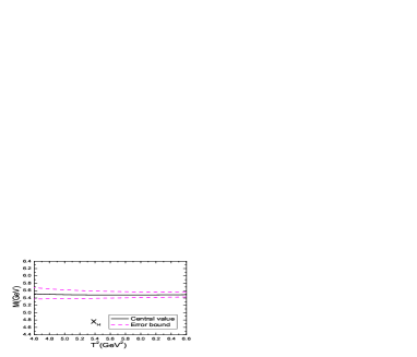
which are also shown in Figs.1-2. In Figs.1-2, we plot the masses and pole residues with variations of the Borel parameters at much larger intervals than the Borel windows shown in Eqs.(27-28). From Eqs.(33-34) and Figs.1-2, we can see that the energy scale formula is satisfied and there appear platforms in the Borel windows, the uncertainties originate from the Borel parameters in the Borel windows are very small, $\delta M_{X_{L}}/M_{X_{L}},\,\delta M_{X_{H}}/M_{X_{H}}\ll 1\%$, while the uncertainties originate from the Borel parameters outside of the Borel windows are rather large compared to the central values, where the criterion $\bf{1}$ or the criterion $\bf{2}$ is not satisfied. In the Borel windows, the four criteria are all satisfied, we expect to make reliable predictions. In calculations, we observe that the predicted masses $M_{X_{L}}$ and $M_{X_{H}}$ decrease monotonously with increase of the energy scales, the uncertainty $\delta\mu=\pm 0.1\,\rm{GeV}$ can lead to uncertainties $\delta M_{X_{L}}=\pm 20\,\rm{MeV}$ and $\delta M_{X_{H}}=\pm 3\,\rm{MeV}$.

The present prediction $M_{X_{L}}=3.89\pm 0.05\,\rm{GeV}$ is compatible with the experimental value $M_{X(3915)}=3918.4\pm 1.9\,\rm{MeV}$ [23], so it is reasonable to assign the $X_{L}$ to be the $X(3915)$. The predicted mass $M_{X_{H}}=5.48\pm 0.10\,\rm{GeV}$ lies above the upper bound of the experimental value $M_{X(4700)}=4704\pm 10^{+14}_{-24}\mbox{ GeV}$, it is impossible to assign the $X(4700)$ to be the $C-C$ type scalar tetraquark state. In Ref.[7], we obtain the values $M_{X(3915)}=3.91^{+0.21}_{-0.17}\,\rm{GeV}$, $M_{X(4500)}=4.50^{+0.08}_{-0.09}\,\rm{GeV}$, $M_{X(4700)}=4.70^{+0.08}_{-0.09}\,\rm{GeV}$, which are in excellent agreement with the experimental data, and support assigning the $X(3915)$ and $X(4500)$ to be the 1S and 2S $C\gamma_{\mu}\otimes\gamma^{\mu}C$ type tetraquark states, and support assigning the $X(4700)$ to be the 1S $C\gamma_{\mu}\gamma_{5}\otimes\gamma_{5}\gamma^{\mu}C$ type tetraquark state.

For the hidden-charm mesons, the energy gaps between the ground states and the first radial excited states are $M_{\psi^{\prime}}-M_{J/\psi}=589\,\rm{MeV}$, $M_{\eta_{c}^{\prime}}-M_{\eta_{c}}=656\,\rm{MeV}$ [23], $M_{Z(4430)}-M_{Z_{c}(3900)}=576\,\rm{MeV}$ [26]. In this article, we choose the continuum threshold parameters as $\sqrt{s^{0}_{L}}-M_{X_{L}}=0.4\sim 0.6\mbox{ GeV}$ and $\sqrt{s^{0}_{H}}-M_{X_{H}}=0.4\sim 0.6\mbox{ GeV}$, the contaminations of the radial excited states can be neglected. On the other hand, the currents $J_{L/H}(x)$ couple potentially to the scattering states $J/\psi\omega$, $J/\psi\phi$, $D_{s}^{*\pm}D_{s}^{*\mp}$, $\cdots$, we can take into account the contributions of the intermediate meson-loops. All the renormalized self-energies contribute a finite imaginary part to modify the dispersion relation, we can take into account the finite width effects by the simple replacement of the hadronic spectral densities,

$\displaystyle\delta\left(s-M^{2}_{L/H}\right)$ $\displaystyle\to$ 1π​s​ΓL/H​(s)(sβˆ’ML/H2)2+s​ΓL/H2​(s).1πœ‹π‘ subscriptΓ𝐿𝐻𝑠superscript𝑠superscriptsubscript𝑀𝐿𝐻22𝑠superscriptsubscriptΓ𝐿𝐻2𝑠\displaystyle\frac{1}{\pi}\frac{\sqrt{s}\,\Gamma_{L/H}(s)}{\left(s-M_{L/H}^{2}\right)^{2}+s\,\Gamma_{L/H}^{2}(s)}\,. (36)

The widths $\Gamma_{X(3915)}=20\pm 5\mbox{ MeV}$ [23] and $\Gamma_{X(4700)}=120\pm 31{}^{+42}_{-33}\mbox{ MeV}$ [1] are not broad, the effects of the finite widths can be absorbed safely into the pole residues [7, 8, 28], the present predictions of the masses are reasonable.

Now we can obtain the conclusion tentatively that the $X(3915)$ maybe have both $C\gamma_{\mu}\otimes\gamma^{\mu}C$ type and $C\gamma_{5}\otimes\gamma_{5}C$ type tetraquark components.

Refer to caption
Refer to caption
Figure 1: The masses $M_{X_{L}}$ and $M_{X_{H}}$ with variations of the Borel parameters $T^{2}$, where the experimental value denotes the experimental value of the mass $M_{X(3915)}$.
Refer to caption
Refer to caption
Figure 2: The pole residues $\lambda_{X_{L}}$ and $\lambda_{X_{H}}$ with variations of the Borel parameters $T^{2}$.

In the following, we perform Fierz re-arrangement to the currents $J_{L}$ and $J_{H}$ both in the color and Dirac-spinor spaces to obtain the results,

$\displaystyle J_{L}$ $\displaystyle=$ $\displaystyle\frac{1}{4}\left\{\,-\bar{c}c\,\bar{s}s+\bar{c}i\gamma_{5}c\,\bar{s}i\gamma_{5}s-\bar{c}\gamma^{\mu}c\,\bar{s}\gamma_{\mu}s-\bar{c}\gamma^{\mu}\gamma_{5}c\,\bar{s}\gamma_{\mu}\gamma_{5}s+\frac{1}{2}\bar{c}\sigma_{\mu\nu}c\,\bar{s}\sigma^{\mu\nu}s\right.$ (37)
$\displaystyle\left.+\bar{c}s\,\bar{s}c-\bar{c}i\gamma_{5}s\,\bar{s}i\gamma_{5}c+\bar{c}\gamma^{\mu}s\,\bar{s}\gamma_{\mu}c+\bar{c}\gamma^{\mu}\gamma_{5}s\,\bar{s}\gamma_{\mu}\gamma_{5}c-\frac{1}{2}\bar{c}\sigma_{\mu\nu}s\,\bar{s}\sigma^{\mu\nu}c\,\right\}\,,$
$\displaystyle J_{H}$ $\displaystyle=$ $\displaystyle\frac{1}{4}\left\{\,\bar{c}i\gamma_{5}c\,\bar{s}i\gamma_{5}s-\bar{c}c\,\bar{s}s+\bar{c}\gamma^{\mu}\gamma_{5}c\,\bar{s}\gamma_{\mu}\gamma_{5}s+\bar{c}\gamma^{\mu}c\,\bar{s}\gamma_{\mu}s+\frac{1}{2}\bar{c}\sigma_{\mu\nu}\gamma_{5}c\,\bar{s}\sigma^{\mu\nu}\gamma_{5}s\right.$ (38)
$\displaystyle\left.+\bar{c}s\,\bar{s}c-\bar{c}i\gamma_{5}s\,\bar{s}i\gamma_{5}c-\bar{c}\gamma^{\mu}s\,\bar{s}\gamma_{\mu}c-\bar{c}\gamma^{\mu}\gamma_{5}s\,\bar{s}\gamma_{\mu}\gamma_{5}c-\frac{1}{2}\bar{c}\sigma_{\mu\nu}s\,\bar{s}\sigma^{\mu\nu}c\,\right\}\,,$

the components couple to the meson pairs, for example, $J/\psi\phi$, $D_{s}\bar{D}_{s}$, $D_{s}^{*}\bar{D}_{s}^{*}$. The two-body strong decays

$\displaystyle X_{L}$ $\displaystyle\to$ $\displaystyle J/\psi\phi\to J/\psi\omega\,\,\,(\phi-\omega\,\,{\rm mixing})\,,$
$\displaystyle X_{H}$ $\displaystyle\to$ $\displaystyle J/\psi\phi\,\,,\,\,D_{s}\bar{D}_{s}\,\,,\,\,D^{*}_{s}\bar{D}^{*}_{s}\,\,,\,\,D_{s0}\bar{D}_{s0}\,\,,\,\,D_{s1}\bar{D}_{s1}$ (39)

are Okubo-Zweig-Iizuka super-allowed. We can search for the $X_{L}$ and $X_{H}$ in those decays in the future. The diquark-antidiquark type tetraquark state can be taken as a special superposition of a series of meson-meson pairs, and embodies the net effects. The decays to its components, for example, $J/\psi\phi$, are Okubo-Zweig-Iizuka super-allowed, but the re-arrangements in the color-space are non-trivial.

3 QCD sum rules for the $X(3915)$ and $X(4500)$ as the $C\gamma_{5}\otimes\gamma_{5}C$ type tetraquark states

Now we tentatively assign the $X(3915)$ and $X(4500)$ to be the 1S and 2S $C\gamma_{5}\otimes\gamma_{5}C$ type tetraquark states, respectively, and study their masses and pole residues with the QCD sum rules. At the phenomenological side, we isolate the 1S and 2S scalar $cs\bar{c}\bar{s}$ tetraquark states in the correlation function Ξ L​(p)subscriptΠ𝐿𝑝\Pi_{L}(p), and get the following result,

Ξ L​(p)subscriptΠ𝐿𝑝\displaystyle\Pi_{L}(p) $\displaystyle=$ $\displaystyle\frac{\lambda_{X_{L}{(\rm 1S)}}^{2}}{M_{X_{L}{(\rm 1S)}}^{2}-p^{2}}+\frac{\lambda_{X_{L}{(\rm 2S)}}^{2}}{M_{X_{L}{(\rm 2S)}}^{2}-p^{2}}+\cdots\,\,,$ (40)

where the pole residues $\lambda_{X_{L}{(\rm 1S,2S)}}$ are defined by $\langle 0|J_{L}(0)|X_{L}{(\rm 1S,2S)}(p)\rangle=\lambda_{X_{L}{(\rm 1S,2S)}}$. As the current $J_{L}(x)$ couples potentially to the scattering states $J/\psi\omega$, $J/\psi\phi$, $D_{s}^{*\pm}D_{s}^{*\mp}$, $\cdots$, which contribute a finite imaginary part to modify the dispersion relation, we can take into account the finite width effects according to Eq.(36), and absorb the finite width effects into the pole residues [7, 8, 28]. The contributions of the scattering states $J/\psi\omega$, $J/\psi\phi$, $D_{s}^{*\pm}D_{s}^{*\mp}$, $\cdots$ can be safely neglected if only the predicted masses $M_{X_{L}{(\rm 1S,2S)}}$ are concerned.

We take into account the contribution of the $X(4500)$ and postpone the continuum threshold $s_{L}^{0}$ to the large value $s_{X(4500)}^{0}$ in the QCD sum rule in Eq.(14) to obtain the QCD sum rule,

Ξ»XL​(1​S)2​exp⁑(βˆ’MXL​(1​S)2T2)+Ξ»XL​(2​S)2​exp⁑(βˆ’MXL​(2​S)2T2)=∫4​mc2sX​(4500)0𝑑s​ρL​(s)​exp⁑(βˆ’sT2),subscriptsuperscriptπœ†2subscript𝑋𝐿1Ssubscriptsuperscript𝑀2subscript𝑋𝐿1Ssuperscript𝑇2subscriptsuperscriptπœ†2subscript𝑋𝐿2Ssubscriptsuperscript𝑀2subscript𝑋𝐿2Ssuperscript𝑇2superscriptsubscript4superscriptsubscriptπ‘šπ‘2superscriptsubscript𝑠𝑋45000differential-d𝑠subscriptπœŒπΏπ‘ π‘ superscript𝑇2\displaystyle\lambda^{2}_{X_{L}{(\rm 1S)}}\,\exp\left(-\frac{M^{2}_{X_{L}{(\rm 1S)}}}{T^{2}}\right)+\lambda^{2}_{X_{L}{(\rm 2S)}}\,\exp\left(-\frac{M^{2}_{X_{L}{(\rm 2S)}}}{T^{2}}\right)=\int_{4m_{c}^{2}}^{s_{X(4500)}^{0}}ds\,\rho_{L}(s)\,\exp\left(-\frac{s}{T^{2}}\right)\,, (41)

then we introduce the notations $\tau=\frac{1}{T^{2}}$, $D^{n}=\left(-\frac{d}{d\tau}\right)^{n}$, and use the subscripts $1$ and $2$ to denote the 1S state $X(3915)$ and the 2S state $X(4500)$ respectively for simplicity. The QCD sum rule can be rewritten as

$\displaystyle\lambda_{1}^{2}\exp\left(-\tau M_{1}^{2}\right)+\lambda_{2}^{2}\exp\left(-\tau M_{2}^{2}\right)$ $\displaystyle=$ Ξ Q​C​D​(Ο„),subscriptΞ π‘„πΆπ·πœ\displaystyle\Pi_{QCD}(\tau)\,, (42)

here we add the subscript $QCD$ to denote the QCD side of the correlation function Ξ L​(Ο„)subscriptΠ𝐿𝜏\Pi_{L}(\tau). We derive the QCD sum rule in Eq.(42) with respect to $\tau$ to obtain

$\displaystyle\lambda_{1}^{2}M_{1}^{2}\exp\left(-\tau M_{1}^{2}\right)+\lambda_{2}^{2}M_{2}^{2}\exp\left(-\tau M_{2}^{2}\right)$ $\displaystyle=$ D​ΠQ​C​D​(Ο„).𝐷subscriptΞ π‘„πΆπ·πœ\displaystyle D\Pi_{QCD}(\tau)\,. (43)

Then we have two equations, and obtain the QCD sum rules,

$\displaystyle\lambda_{i}^{2}\exp\left(-\tau M_{i}^{2}\right)$ $\displaystyle=$ (Dβˆ’Mj2)​ΠQ​C​D​(Ο„)Mi2βˆ’Mj2,𝐷superscriptsubscript𝑀𝑗2subscriptΞ π‘„πΆπ·πœsuperscriptsubscript𝑀𝑖2superscriptsubscript𝑀𝑗2\displaystyle\frac{\left(D-M_{j}^{2}\right)\Pi_{QCD}(\tau)}{M_{i}^{2}-M_{j}^{2}}\,, (44)

where iβ‰ j𝑖𝑗i\neq j. Now we derive the QCD sum rules in Eq.(44) with respect to $\tau$ to obtain

$\displaystyle M_{i}^{2}$ $\displaystyle=$ (D2βˆ’Mj2​D)​ΠQ​C​D​(Ο„)(Dβˆ’Mj2)​ΠQ​C​D​(Ο„),superscript𝐷2superscriptsubscript𝑀𝑗2𝐷subscriptΞ π‘„πΆπ·πœπ·superscriptsubscript𝑀𝑗2subscriptΞ π‘„πΆπ·πœ\displaystyle\frac{\left(D^{2}-M_{j}^{2}D\right)\Pi_{QCD}(\tau)}{\left(D-M_{j}^{2}\right)\Pi_{QCD}(\tau)}\,,
$\displaystyle M_{i}^{4}$ $\displaystyle=$ (D3βˆ’Mj2​D2)​ΠQ​C​D​(Ο„)(Dβˆ’Mj2)​ΠQ​C​D​(Ο„).superscript𝐷3superscriptsubscript𝑀𝑗2superscript𝐷2subscriptΞ π‘„πΆπ·πœπ·superscriptsubscript𝑀𝑗2subscriptΞ π‘„πΆπ·πœ\displaystyle\frac{\left(D^{3}-M_{j}^{2}D^{2}\right)\Pi_{QCD}(\tau)}{\left(D-M_{j}^{2}\right)\Pi_{QCD}(\tau)}\,. (45)

The squared masses $M_{i}^{2}$ satisfy the following equation,

$\displaystyle M_{i}^{4}-bM_{i}^{2}+c$ $\displaystyle=$ $\displaystyle 0\,,$ (46)

where

$\displaystyle b$ $\displaystyle=$ $\displaystyle\frac{D^{3}\otimes D^{0}-D^{2}\otimes D}{D^{2}\otimes D^{0}-D\otimes D}\,,$
$\displaystyle c$ $\displaystyle=$ $\displaystyle\frac{D^{3}\otimes D-D^{2}\otimes D^{2}}{D^{2}\otimes D^{0}-D\otimes D}\,,$
$\displaystyle D^{j}\otimes D^{k}$ $\displaystyle=$ Dj​ΠQ​C​D​(Ο„)​Dk​ΠQ​C​D​(Ο„),superscript𝐷𝑗subscriptΞ π‘„πΆπ·πœsuperscriptπ·π‘˜subscriptΞ π‘„πΆπ·πœ\displaystyle D^{j}\Pi_{QCD}(\tau)\,D^{k}\Pi_{QCD}(\tau)\,, (47)

$i=1,2$, $j,k=0,1,2,3$. We solve the equation in Eq.(46) and obtain the solutions

$\displaystyle M_{1}^{2}=\frac{b-\sqrt{b^{2}-4c}}{2}\,,$ (48)
$\displaystyle M_{2}^{2}=\frac{b+\sqrt{b^{2}-4c}}{2}\,.$ (49)

In Ref.[27], M. S. Maior de Sousa and R. Rodrigues da Silva study the masses and decay constants of the $\rho({\rm 1S,2S})$, $\psi({\rm 1S,2S})$, $\Upsilon({\rm 1S,2S})$ using Eqs.(48-49), and observe that the ground state masses are (much) smaller than the experimental values. In Ref.[26], we apply this approach to study the $Z_{c}(3900)$ and $Z(4430)$ as the 1S and 2S axialvector hidden-charm tetraquark states, respectively, and use the energy scale formula $\mu=\sqrt{M^{2}_{X/Y/Z}-(2{\mathbb{M}}_{c})^{2}}$ to overcome the shortcoming [27], and reproduce the experimental values of the masses $M_{Z_{c}(3900)}$ and $M_{Z(4430)}$. In Ref.[7], we use the same approach to study the $X(3915)$ and $X(4500)$ as the 1S and 2S $C\gamma_{\mu}\otimes\gamma^{\mu}C$ type scalar $cs\bar{c}\bar{s}$ tetraquark states, respectively, and reproduce the experimental values of the masses $M_{X(3915)}$ and $M_{X(4500)}$. Now we tentatively assign the $X(3915)$ and $X(4500)$ to be the 1S and 2S $C\gamma_{5}\otimes\gamma_{5}C$ type tetraquark states, respectively, and resort to the same approach study the masses and pole residues with the QCD sum rules.

Again, we search for the Borel parameter $T^{2}$ and continuum threshold parameter $s^{0}_{X(4500)}$ according to the four criteria:

$\bf{1_{\cdot}}$ Pole dominance at the phenomenological side;

$\bf{2_{\cdot}}$ Convergence of the operator product expansion;

$\bf{3_{\cdot}}$ Appearance of the Borel platforms;

$\bf{4_{\cdot}}$ Satisfying the energy scale formula.
The resulting Borel parameter and threshold parameter are

$\displaystyle X(3890/4350)$ $\displaystyle:$ $\displaystyle T^{2}=(1.8-2.2)\mbox{ GeV}^{2}\,,\,s^{0}_{X(4350)}=(4.9\pm 0.1\mbox{ GeV})^{2}\,,$ (50)

here we use the notations $3890$ and $4350$ in stead of $3915$ and $4500$ according to the masses extracted from the QCD sum rules. The pole contributions are

$\displaystyle X(3890)+X(4350)$ $\displaystyle:$ $\displaystyle{\rm pole}=(87-98)\%\,\,\,{\rm at}\,\,\,\mu=1.25\mbox{ GeV}\,,$ (51)
$\displaystyle X(3890)+X(4350)$ $\displaystyle:$ $\displaystyle{\rm pole}=(93-99)\%\,\,\,{\rm at}\,\,\,\mu=2.40\mbox{ GeV}\,,$ (52)

the pole dominance condition is well satisfied. The contributions come from the vacuum condensates of dimension 10 $D_{10}$ are

$\displaystyle X(3890)+X(4350)$ $\displaystyle:$ $\displaystyle D_{10}=(1-3)\%\,\,\,{\rm at}\,\,\,\mu=1.25\mbox{ GeV}\,,$ (53)
$\displaystyle X(3890)+X(4350)$ $\displaystyle:$ $\displaystyle D_{10}=(0-1)\%\,\,\,{\rm at}\,\,\,\mu=2.40\mbox{ GeV}\,,$ (54)

the operator product expansion is well convergent.

Now we take into account uncertainties of all the input parameters, and obtain the masses and pole residues of the $X(3890)$ and $X(4350)$,

$\displaystyle M_{X(3890)}$ $\displaystyle=$ 3.85βˆ’0.17+0.18​GeV,Experimental​value​    3918.4Β±1.9​MeV​[23],subscriptsuperscript3.850.180.17GeVplus-or-minusExperimentalvalue3918.41.9MeV[23]\displaystyle 3.85^{+0.18}_{-0.17}\,\rm{GeV}\,,\,\,\,{\rm Experimental\,\,value}\,\,\,\,3918.4\pm 1.9\,\rm{MeV}\,\cite[cite]{[\@@bibref{}{PDG}{}{}]}\,,
$\displaystyle M_{X(4350)}$ $\displaystyle=$ $\displaystyle 4.83\,\rm{GeV}\,,$
$\displaystyle\lambda_{X(3890)}$ $\displaystyle=$ $\displaystyle 1.84^{+0.76}_{-0.54}\times 10^{-2}\,\rm{GeV}^{5}\,,$
$\displaystyle\lambda_{X(4350)}$ $\displaystyle=$ $\displaystyle 5.82\times 10^{-2}\,\rm{GeV}^{5}\,,$ (55)

at the energy scale $\mu=1.25\,\rm{GeV}$,

$\displaystyle M_{X(3890)}$ $\displaystyle=$ $\displaystyle 3.29\,\rm{GeV}\,,$
$\displaystyle M_{X(4350)}$ $\displaystyle=$ 4.35βˆ’0.11+0.10​GeV,Experimental​value​    4506Β±11βˆ’15+12​MeV​[1],subscriptsuperscript4.350.100.11GeVplus-or-minusExperimentalvalue4506subscriptsuperscript111215MeV[1]\displaystyle 4.35^{+0.10}_{-0.11}\,\rm{GeV}\,,\,\,\,{\rm Experimental\,\,value}\,\,\,\,4506\pm 11^{+12}_{-15}\,\rm{MeV}\,\cite[cite]{[\@@bibref{}{LHCb-4500-1606}{}{}]}\,,
$\displaystyle\lambda_{X(3890)}$ $\displaystyle=$ $\displaystyle 1.16\times 10^{-2}\,\rm{GeV}^{5}\,,$
$\displaystyle\lambda_{X(4350)}$ $\displaystyle=$ $\displaystyle 6.01^{+0.93}_{-0.80}\times 10^{-2}\,\rm{GeV}^{5}\,,$ (56)

at the energy scale $\mu=2.40\,\rm{GeV}$, where we have neglected the uncertainties out of control.
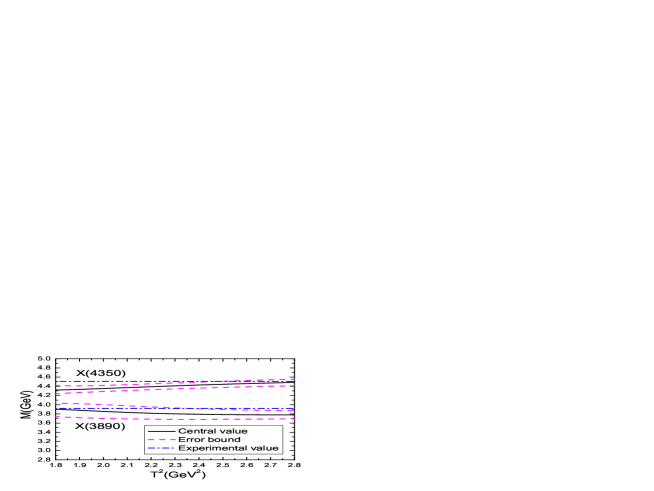
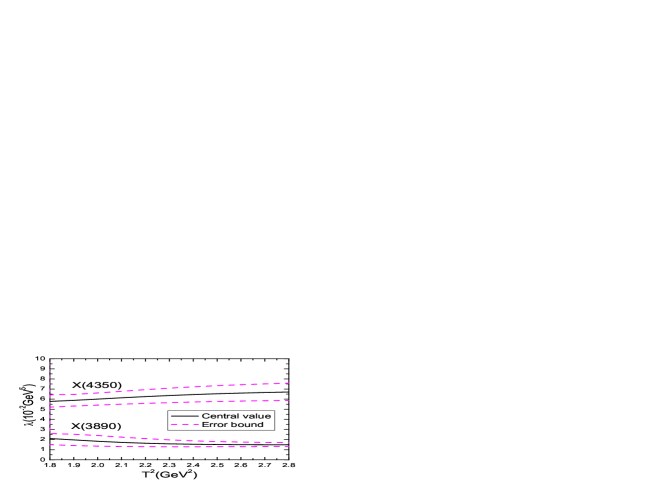
Refer to caption
Figure 3: The masses $M_{X(3890)}$ and $M_{X(4350)}$ with variations of the Borel parameters $T^{2}$, where the experimental value denotes the experimental values of the masses $M_{X(3915)}$ and $M_{X(4500)}$.
Refer to caption
Figure 4: The residues $\lambda_{X(3890)}$ and $\lambda_{X(4350)}$ with variations of the Borel parameters $T^{2}$.

Then we take the central values of the masses and pole residues as the input parameters, and obtain the pole contributions of the $X(3890)$ and $X(4350)$ respectively,

$\displaystyle{\rm pole}_{X(3890)}$ $\displaystyle=$ $\displaystyle(72-90)\%\,,$
$\displaystyle{\rm pole}_{X(4350)}$ $\displaystyle=$ $\displaystyle(8-15)\%\,,$ (57)

at the energy scale $\mu=1.25\,\rm{GeV}$ and

$\displaystyle{\rm pole}_{X(3890)}$ $\displaystyle=$ $\displaystyle(55-76)\%\,,$
$\displaystyle{\rm pole}_{X(4350)}$ $\displaystyle=$ $\displaystyle(23-38)\%\,,$ (58)

at the energy scale $\mu=2.40\,\rm{GeV}$.

The pole contribution of the $X(3890/4350)$ at $\mu=1.25/2.40\,\rm{GeV}$ is larger than that at $\mu=2.40/1.25\,\rm{GeV}$, we prefer to extract the mass and pole residue of the $X(3890/4350)$ from the QCD spectral density at $\mu=1.25/2.40\,\rm{GeV}$ and neglect the ones at $\mu=2.40/1.25\,\rm{GeV}$. The neglected values of the masses do not satisfy the energy scale formula in Eq.(2). In this article, we choose the values

$\displaystyle M_{X(3890)}$ $\displaystyle=$ 3.85βˆ’0.17+0.18​GeV,Experimental​value​    3918.4Β±1.9​MeV​[23],subscriptsuperscript3.850.180.17GeVplus-or-minusExperimentalvalue3918.41.9MeV[23]\displaystyle 3.85^{+0.18}_{-0.17}\,\rm{GeV}\,,\,\,\,{\rm Experimental\,\,value}\,\,\,\,3918.4\pm 1.9\,\rm{MeV}\,\cite[cite]{[\@@bibref{}{PDG}{}{}]}\,,
$\displaystyle M_{X(4350)}$ $\displaystyle=$ 4.35βˆ’0.11+0.10​GeV,Experimental​value​    4506Β±11βˆ’15+12​MeV​[1],subscriptsuperscript4.350.100.11GeVplus-or-minusExperimentalvalue4506subscriptsuperscript111215MeV[1]\displaystyle 4.35^{+0.10}_{-0.11}\,\rm{GeV}\,,\,\,\,{\rm Experimental\,\,value}\,\,\,\,4506\pm 11^{+12}_{-15}\,\rm{MeV}\,\cite[cite]{[\@@bibref{}{LHCb-4500-1606}{}{}]}\,, (59)
$\displaystyle\lambda_{X(3890)}$ $\displaystyle=$ $\displaystyle 1.84^{+0.76}_{-0.54}\times 10^{-2}\,\rm{GeV}^{5}\,,$
$\displaystyle\lambda_{X(4350)}$ $\displaystyle=$ $\displaystyle 6.01^{+0.93}_{-0.80}\times 10^{-2}\,\rm{GeV}^{5}\,,$ (60)

which are also shown in Figs.3-4. In Figs.3-4, we plot the masses and pole residues with variations of the Borel parameter $T^{2}$ at much larger interval than the Borel window shown in Eq.(50). There appear platforms not very flat in the Borel window, which result in uncertainties $\delta M_{X_{L}}/M_{X_{L}},\,\delta M_{X_{H}}/M_{X_{H}}=\pm 1\%$, while the uncertainties originate from the Borel parameter outside of the Borel window are rather large compared to the central values. The predicted masses $M_{X(3890)}=3.85^{+0.18}_{-0.17}\,\rm{GeV}$ and $M_{X(4350)}=4.35^{+0.10}_{-0.11}\,\rm{GeV}$ satisfy the energy scale formula. From Fig.3, we can see that the predicted mass $M_{X(3890)}=3.85^{+0.18}_{-0.17}\,\rm{GeV}$ is compatible with the experimental value $M_{X(3915)}=3918.4\pm 1.9\,\rm{MeV}$ [23], so it is reasonable to assign the $X(3890)$ to be the $X(3915)$. The predicted mass $M_{X(4350)}=4.35^{+0.10}_{-0.11}\,\rm{GeV}$ lies below the lower bound of the experimental value $M_{X(4500)}=4506\pm 11^{+12}_{-15}\,\rm{MeV}$ [1], it is not favored to assign the $X(4500)$ to be the 2S $C\gamma_{5}\otimes\gamma_{5}C$ type scalar tetraquark state. Now we can draw the conclusion tentatively that the $X(3915)$ maybe have both $C\gamma_{\mu}\otimes\gamma^{\mu}C$ type and $C\gamma_{5}\otimes\gamma_{5}C$ type tetraquark components, while the $X(4500)$ can be assigned to the 2S $C\gamma_{\mu}\otimes\gamma^{\mu}C$ type tetraquark state [7].

In the Borel or Laplace QCD sum rules, we introduce a new parameter $T^{2}$ therefore an exponential factor $\exp\left(-\frac{s}{T^{2}}\right)$ to suppress the experimentally unknown higher resonances. The Borel parameter $T^{2}$ has no physical significance other than being a mathematical artifact, leads to rather narrow stability window for the hidden charm or hidden bottom tetraquark states. On the other hand, the continuum threshold $s_{0}$, which has a clear physical interpretation, is often exponentially suppressed $\exp\left(-\frac{s_{0}}{T^{2}}\right)$, or at best reduced in importance [29]. While in the finite energy QCD sum rules or Hilbert moment QCD sum rules, the threshold $s_{0}$ shows a power-like welcome feature, it is interesting to study the hidden charm or hidden bottom tetraquark states with the finite energy QCD sum rules or Hilbert moment QCD sum rules, this may be our next work.

4 Conclusion

In this article, we study the $C\gamma_{5}\otimes\gamma_{5}C$ type and $C\otimes C$ type scalar $cs\bar{c}\bar{s}$ tetraquark states with the QCD sum rules by calculating the contributions of the vacuum condensates up to dimension 10 in a consistent way. In calculations, we use the energy scale formula $\mu=\sqrt{M^{2}_{X/Y/Z}-(2{\mathbb{M}}_{c})^{2}}$ to determine the optimal energy scales of the QCD spectral densities. The ground state masses $M_{C\gamma_{5}\otimes\gamma_{5}C}=3.89\pm 0.05\,\rm{GeV}$ and $M_{C\otimes C}=5.48\pm 0.10\,\rm{GeV}$ support assigning the $X(3915)$ to be the 1S $C\gamma_{5}\otimes\gamma_{5}C$ type tetraquark state with $J^{PC}=0^{++}$, but do not support assigning the $X(4700)$ to be the 1S $C\otimes C$ type $cs\bar{c}\bar{s}$ tetraquark state with $J^{PC}=0^{++}$. Then we tentatively assign the $X(3915)$ and $X(4500)$ to be the $\rm 1S$ and $\rm 2S$ $C\gamma_{5}\otimes\gamma_{5}C$ type scalar $cs\bar{c}\bar{s}$ tetraquark states respectively, and obtain the $\rm{1S}$ mass $M_{\rm 1S}=3.85^{+0.18}_{-0.17}\,\rm{GeV}$ and $\rm{2S}$ mass $M_{\rm 2S}=4.35^{+0.10}_{-0.11}\,\rm{GeV}$ from the QCD sum rules, which support assigning the $X(3915)$ to be the $\rm{1S}$ $C\gamma_{5}\otimes\gamma_{5}C$ type tetraquark state, but do not support assigning the $X(4500)$ to be the ${\rm 2S}$ $C\gamma_{5}\otimes\gamma_{5}C$ type tetraquark state. The $X(3915)$ maybe have both $C\gamma_{\mu}\otimes\gamma^{\mu}C$ type and $C\gamma_{5}\otimes\gamma_{5}C$ type tetraquark components, while the $X(4500)$ can be assigned to the 2S $C\gamma_{\mu}\otimes\gamma^{\mu}C$ type tetraquark state.

Acknowledgements

This work is supported by National Natural Science Foundation, Grant Numbers 11375063, and Natural Science Foundation of Hebei province, Grant Number A2014502017.

References

  • [1] R. Aaij et al, arXiv:1606.07895; R. Aaij et al, arXiv:1606.07898.
  • [2] H. X. Chen, E. L. Cui, W. Chen, X. Liu and S. L. Zhu, arXiv:1606.03179.
  • [3] X. H. Liu, arXiv:1607.01385.
  • [4] L. Maiani, A. D. Polosa and V. Riquer, Phys. Rev. D94 (2016) 054026.
  • [5] R. Zhu, Phys. Rev. D94 (2016) 054009.
  • [6] R. F. Lebed and A. D. Polosa, Phys. Rev. D93 (2016) 094024.
  • [7] Z. G. Wang, arXiv:1606.05872.
  • [8] Z. G. Wang, Eur. Phys. J. C76 (2016) 657.
  • [9] A. De Rujula, H. Georgi and S. L. Glashow, Phys. Rev. D12 (1975) 147; T. DeGrand, R. L. Jaffe, K. Johnson and J. E. Kiskis, Phys. Rev. D12 (1975) 2060.
  • [10] Z. G. Wang, Eur. Phys. J. C71 (2011) 1524; R. T. Kleiv, T. G. Steele and A. Zhang, Phys. Rev. D87 (2013) 125018.
  • [11] Z. G. Wang, Commun. Theor. Phys. 59 (2013) 451.
  • [12] Z. G. Wang, Phys. Rev. D79 (2009) 094027; Z. G. Wang, Eur. Phys. J. C67 (2010) 411.
  • [13] Z. G. Wang, Eur. Phys. J. C74 (2014) 2874.
  • [14] Z. G. Wang, Commun. Theor. Phys. 63 (2015) 466.
  • [15] Z. G. Wang and T. Huang, Nucl. Phys. A930 (2014) 63.
  • [16] M. A. Shifman, A. I. Vainshtein and V. I. Zakharov, Nucl. Phys. B147 (1979) 385; Nucl. Phys. B147 (1979) 448.
  • [17] L. J. Reinders, H. Rubinstein and S. Yazaki, Phys. Rept. 127 (1985) 1.
  • [18] P. Pascual and R. Tarrach, β€œQCD: Renormalization for the practitioner”, Springer Berlin Heidelberg (1984).
  • [19] Z. G. Wang and T. Huang, Phys. Rev. D89 (2014) 054019.
  • [20] Z. G. Wang, Acta Phys. Polon. B44 (2013) 1971; Z. G. Wang, Eur. Phys. J. A49 (2013) 131.
  • [21] P. Colangelo and A. Khodjamirian, hep-ph/0010175.
  • [22] S. Narison, Camb. Monogr. Part. Phys. Nucl. Phys. Cosmol. 17 (2002) 1.
  • [23] C. Patrignani et al, Chin. Phys. C40 (2016) 100001.
  • [24] S. J. Brodsky, D. S. Hwang and R. F. Lebed, Phys. Rev. Lett. 113 (2014) 112001.
  • [25] Z. G. Wang, Eur. Phys. J. C76 (2016) 387.
  • [26] Z. G. Wang, Commun. Theor. Phys. 63 (2015) 325.
  • [27] M. S. Maior de Sousa and R. Rodrigues da Silva, Braz. J. Phys. 46 (2016) 730.
  • [28] Z. G. Wang, Int. J. Theor. Phys. 51 (2012) 507; Z. G. Wang, Int. J. Mod. Phys. A30 (2015) 1550168.
  • [29] C. A. Dominguez, Int. J. Mod. Phys. A29 (2014) 1430069; A. Ayala, C. A. Dominguez and M. Loewe, arXiv:1608.04284.