Kauffman type invariants for tied links

Abstract.

We define two new invariants for tied links. One of them can be thought as an extension of the Kauffman polynomial and the other one as an extension of the Jones polynomial which is constructed via a bracket polynomial for tied links. These invariants are more powerful than both the Kauffman and the bracket polynomials when evaluated on classical links. Further, the extension of the Kauffman polynomial is more powerful of the Homflypt polynomial, as well as of certain new invariants introduced recently. Also we propose a new algebra which plays in the case of tied links the same role as the BMW algebra for the Kauffman polynomial in the classical case. Moreover, we prove that the Markov trace on this new algebra can be recovered from the extension of the Kauffman polynomial defined here.

1. Introduction

The tied links constitute a class of knot–like objects, introduced by the authors in [3], which contains the classical links. The original motivation to introduce these objects arose from the diagrammatical interpretation of the defining generators of the so–called algebra of braids and ties or simply bt–algebra, see [1, 2, 3].

Tied links are no other than classical links whose set of components is partitioned into subsets: two components connected by one or more ties belong to the same subset of the partition.

A tied link diagram is like the diagram of a link, provided with ties, depicted as springs connecting pairs of points lying on the curves. Classical links can be considered either tied links with no ties between different components (i.e., each subset of the partition contains one component) or tied links whose components are all tied together. Of course, classical knots coincide in both cases with tied knots.

In [3] an invariant for tied links, denoted ${\mathcal{F}}$, is defined by skein relations. This invariant can be regarded as an extension of the Homflypt polynomial, since it coincides with the Homflypt polynomial when evaluated on knots and classical links, provided that they are considered as tied links with all components tied together.

Notice that tied links play an important role also in the definition of an invariant $\Theta$ for classical links which is a generalization of certain invariants derived from the Yokonuma–Hecke algebra [8]. The invariant $\Theta$ on links is more powerful of the Homflypt polynomial, for details see [8, Section 8].

Also notice that the invariant $\mathcal{F}$ provides, too, an invariant of links more powerful than the Homflypt polynomial, when evaluated on tied links without ties [4].

The invariant $\mathcal{F}$ can be also constructed through the Jones recipe . In fact, we have proved that the bt–algebra supports a Markov trace [2], and that $\mathcal{F}$ can be obtained as well by the Jones recipe applied to the bt–algebra. To do this, we have introduced the algebraic counterpart of the braid group for tied links, that is the tied braids monoid, and we have proved the analogous of Alexander and Markov theorems for tied links; for details see [3].

Since the invariant $\mathcal{F}$ can be thought as the Homflypt polynomial for tied links, it is quite natural the question whether a generalization of the Kauffman polynomial [15] can be defined for tied links. This paper proposes and studies a Kauffman polynomial for unoriented (respectively oriented) tied links, denoted by $\mathcal{L}$ (respectively, denoted by $\widehat{\mathcal{L}}$). We also define a sort of Jones polynomial for tied links, and we construct $\widehat{\mathcal{L}}$ through the Jones recipe applied to a suitable ‘tied BMW algebra’. Finally, using data from [6], we show pairs of non–equivalent oriented links which are not distinguished by the Hompflypt polynomial, nor by the Kauffman polynomial, but that are distinguished by $\widehat{\mathcal{L}}$; moreover the invariant $\mathcal{L}$ distinguishes pairs of oriented links that are not distinguished by the invariant $\mathcal{F}$ and $\Theta$.

This paper is organized as follows. Section 2 is dedicated to give the background and notation used in the paper. In Section 3, Theorem 1 proves the existence of the polynomial $\mathcal{L}$. This polynomial is a three variable invariant obtained by modifying suitably the Kauffman skein relations [15, Definition 2.2], that define the Kauffman polynomial $L$ for unoriented links. The polynomial $\mathcal{L}$ coincides with the polynomial $L$ on links whose components are all tied together; in particular, the polynomials $\mathcal{L}$ and $L$ coincide on knots. Moreover, in Theorem 2 we give the invariant of oriented tied links $\widehat{\mathcal{L}}$ associated to $\mathcal{L}$. This is done by using the same normalization originally used to define the Kauffman polynomial for oriented links [15, Lemma 2.1], denoted by $\widehat{L}$, associated to $L$.

Section 4 is devoted to define a bracket polynomial $\langle\langle\quad\rangle\rangle$ for tied links. In Proposition 3 we prove that there exists a two variable generalization $\langle\langle\quad\rangle\rangle$ for unoriented tied links of the one variable bracket polynomial [14]. The polynomial $\langle\langle\quad\rangle\rangle$ becomes the bracket polynomial on links whose components are all tied together, and then coincides with the bracket polynomial on knots. We note that $\langle\langle\quad\rangle\rangle$ results to be a specialization of $\mathcal{L}$. Further, we obtain a generalization of the Jones polynomial for tied links, see Corollary 1.

We start Section 5 by introducing a sort of tied BMW algebra with the aim of recovering the invariant $\widehat{\mathcal{L}}$ via the Jones recipe. In Section 5.1 this tied BMW algebra, called t–BMW algebra, is defined by generators and relations; more precisely, the defining generators are of four types: usual braid generators, tangle generators, tied generators and a new class of objects called tied–tangles generators. The defining relations of the t–BMW algebra are chosen to fulfill the same monomial relations of the bt–algebra [3, 2], the monomial relations of the BMW algebra, together with a suitable tied version of all defining relations of the BMW algebra. In Section 5.2 we show that the diagrammatical interpretations of the defining generators of the t–BMW algebra agrees with the defining relations of it. In Proposition 2, we prove that the t–BMW algebra is finite dimensional, by showing that every element in it can be put in a certain reduced form. This result, together with the existence of the invariant $\mathcal{L}$, allows us to prove that the t–BMW algebra supports a Markov trace, that we denote by $\varpi$. This trace is in fact similar, cf. (46), to the Markov trace $\tau^{\prime}$ on the BMW algebra by Birman and Wenzl [5]; thus, we obtain $\widehat{\mathcal{L}}$ by the Jones recipe. We finish Section 6 by re–proving the fact that $\widehat{L}$ can be obtained as a ‘specialization’ of $\widehat{\mathcal{L}}$, see Proposition 4. The proof of this proposition is completely algebraic and uses the natural homomorphism from the t–BMW algebra onto the BMW algebra and the respective factorization of the trace $\varpi$ by the trace $\tau^{\prime}$, for details see Proposition 3.

A motivation to construct $\mathcal{L}$ was the hope of finding an invariant more powerful than the Kauffman polynomial when calculated on classical links (tied links without ties); in fact we have got that; surprisingly, the polynomial $\langle\langle\quad\rangle\rangle$, too, is more powerful than the Kauffman polynomial. In Section 7 we give an example of pairs of non isotopic oriented links distinguished by both normalizations of $\mathcal{L}$ and $\langle\langle\quad\rangle\rangle$, which are not distinguished by the Homflypt polynomial nor by the Kauffman polynomial. Moreover, the invariant $\mathcal{L}$ distinguishes pairs which are not distinguished by the invariants $\mathcal{F}$ and $\Theta$.

2. Notations and background

2.1.

Tied Links. Recall a tied link is a link whose components may be connected by ties. In fact, classical links form a subset of the set of tied links. The ties of a tied link define a partition of the set of its components: two components connected by one or more ties belong to the same set of the partition. Two tied links are tie–isotopic if they are ambient isotopic and if the ties define the same partition of the set of components.

A tie is depicted as a spring connecting two points of a link. However, a tie is not a topological entity: arcs and other ties can cross through it. The tie–isotopy says that, when remaining in the same equivalence class, it is allowed to move any tie between two components letting its extremes move along the two whole components; moreover, ties can be destroyed or created between two components, provided that these components either coincide, or belong to the same class.

Two components will be said tied together, if they belong to the same subset, i.e., if between them a tie already exists or a tie can be created.

A tie that cannot be destroyed without changing the tie–isotopy class is said essential. Any tie connecting two points of the same component is not essential.

Here we consider diagrams of unoriented tied links in $S^{2}$. Tie–regular isotopic tied links diagrams are evidently regular isotopic links having ties that define the same partition of the set of components.

Two diagrams of tied links are said to be regularly isotopic if one of them can be carried in the other by using the Reidemeister moves II and/or III, as in the classical case.

In what follows the tie–isotopy class of a tied link will be not distinguished from the class of its diagrams.

2.2.

Let $D$ be an unoriented tied link diagram, and let     be the zero crossing diagram of the unknotted circle. We indicate by $D\sqcup\put(6.0,4.0){\circle{8.0}}\quad$ the disjoint union of $D$ with    , and by $D\ \widetilde{\sqcup}\ \put(8.0,4.0){\circle{8.0}}\quad$ the disjoint union of $D$ with    , but in this case there is a tie between $D$ and    .

Moreover, we indicate by $D_{+}$, $D_{-}$, $D_{e}$ and $D_{f}$ four unoriented tied link diagrams that are identical except for a disk in which they look, respectively, as , , , and . The last two diagrams without ties in the selected disc are indicated by $D_{0}$ and $D_{\infty}$.

Let $\overrightarrow{D}$ be an oriented tied link diagrams. We denote by $D$ the unoriented tied link associated to $\overrightarrow{D}$ and we denote by $w(D)$ the writhe of $\overrightarrow{D}$.

2.3.

Let now $\overrightarrow{D}$ be a tied link whose components are all tied together. Any tied link tie–isotopic to $\overrightarrow{D}$ has the components all tied, too; hence, the tie–isotopy of tied links having all components tied together depends only of the isotopy in $S^{2}$. Therefore, the classical links are in topological bijection with the tied links having all components tied together; we shall denote by $\overrightarrow{D}^{\nsim}$ the classical link obtained by forgetting all ties in $\overrightarrow{D}$.

Recall that every tied link can be obtained as the closure of a tied braid, see [3, Theorem 3.5]. The set of tied braids with $n$ strands forms a monoid, denoted $TB_{n}$, which has a presentation with usual braids $\sigma_{1},\ldots,\sigma_{n-1}$ and ties generators $\eta_{1},\ldots,\eta_{n-1}$ and certain relations, for details see [3, Definition 3.1]. The tied monoid $TB_{n}$ is related to the set of the tied links as the braid group $B_{n}$ to the classical links, see [3]. In this last paper was also introduced the exponent of a tied braid $\theta\in TB_{n}$, denoted ${\rm exp}(\theta)$. More precisely, if $\theta$ is the product $\theta_{1}\cdots\theta_{k}$ in the defining generators of $TB_{n}$, then

$${\rm exp}(\theta)=\sum_{i=1}^{r}k_{i},$$

where $k_{i}=\pm 1$ if $\theta_{i}=\sigma_{i}^{\pm 1}$ and $k_{i}=0$ if $\theta_{i}=\eta_{i}$. Notice that if $\overrightarrow{D}$ is the oriented tied link obtained by closing the tied braid $\theta$, then

$$w(D)={\rm exp}(\theta).$$

Further, we define $EB_{n}$ as the subset of $TB_{n}$ formed by the tied braids of the form:

$$\eta^{n}\sigma\quad\text{where}\quad\eta^{n}:=\eta_{1}\cdots\eta_{n-1}\quad\text{and}\quad\sigma\in B_{n}.$$

The closures of the tied braids of $EB_{n}$ correspond to tied links in which the components are all tied together. Notice that

$${\rm exp}(\eta^{n}\sigma)={\rm exp}(\sigma)\quad\text{where}\quad\sigma\in B_{n}.$$

We observe that the monoid $EB_{n}$ is in fact a group, with identity $\eta^{n}$, which is naturally isomorphic to the braid group $B_{n}$; we shall call $\mathtt{f}_{n}$ this natural group isomorphism,

(1) $$\mathtt{f}_{n}:\eta^{n}\sigma\mapsto\sigma.$$

Hence, there is a braid–identification of the set of tied links whose components are all tied together with the set of classical links. Thus, for $\overrightarrow{D}=\widehat{\eta^{n}\sigma}$, we have:

$$\overrightarrow{D}^{\nsim}=\widehat{\sigma},$$

where $\widehat{\sigma}$ is the closure of $\sigma$.

2.4.

Let $K$ be a field. The expression $A$ is a $K$–algebra means that $A$ is an associative $K$–algebra with unity equal to $1$; so, we consider $K$ as contained in the center of $A$.

Along this paper, $a,x$ and $z$ indicate three commutative variables.

3. Kauffman polynomial for tied links

3.1. Definition of $\mathcal{L}$

Theorem 1.

There exists a unique function

$$\mathcal{L}:\{\text{Unoriented tied links diagrams }\}\rightarrow\mathbb{Z}[a^{\pm 1},z^{\pm 1},x^{-1}]$$

that is defined by the following rules:

• $\mathcal{L}(\put(6.0,4.0){\circle{8.0}}\quad)=1$,

• $\mathcal{L}(D\sqcup\put(6.0,4.0){\circle{8.0}}\quad)=x^{-1}\mathcal{L}(D)$,

• $\mathcal{L}$ is invariant under Reidemeister moves II and III,

• $\mathcal{L}(\includegraphics[scale={0.5},trim=0.0pt 11.38092pt 0.0pt 0.0pt]{loop1.pdf})=a\mathcal{L}(\includegraphics[scale={0.5},trim=0.0pt 0.0pt 0.0pt 0.0pt]{loopno.pdf})$,

• $\mathcal{L}(\includegraphics[scale={0.5},trim=0.0pt 11.38092pt 0.0pt 0.0pt]{loop2.pdf})=a^{-1}\mathcal{L}(\includegraphics[scale={0.5}]{loopno.pdf})$,

• $\mathcal{L}(\includegraphics[scale={0.5},trim=0.0pt 11.38092pt 0.0pt 0.0pt]{crossp.pdf})+\mathcal{L}(\includegraphics[scale={0.5},trim=0.0pt 11.38092pt 0.0pt 0.0pt]{crossm.pdf})=z\left(\mathcal{L}(\includegraphics[scale={0.5},trim=0.0pt 11.38092pt 0.0pt 0.0pt]{tanver.pdf})+\mathcal{L}(\includegraphics[scale={0.5},trim=0.0pt 11.38092pt 0.0pt 0.0pt]{tanor.pdf})\right),$

where, as usual, $\mathcal{L}(\includegraphics[scale={0.5},trim=0.0pt 11.38092pt 0.0pt 0.0pt]{crossp.pdf})$, $\mathcal{L}(\includegraphics[scale={0.5},trim=0.0pt 11.38092pt 0.0pt 0.0pt]{crossm.pdf})$, etc., indicate the value of $\mathcal{L}$ on diagrams that are identical except for a disc inside which they look like the pictures in parentheses.

Remark 1.

The analogous of relation (ii) in presence of a tie follows from (iv), (v) and (vi):

(2) $$\mathcal{L}(D\ \widetilde{\sqcup}\ \put(8.0,4.0){\circle{8.0}}\quad)=y\mathcal{L}(D),$$

where

(3) $$y:=(a+a^{-1})z^{-1}-1.$$

Following exactly the same arguments as in [14], we can deduce from $\mathcal{L}$ a tie–isotopic invariant of oriented links, as the next theorem states.

Theorem 2.

Let $\overrightarrow{D}$ be an oriented diagram of a tied link. Then the map $\widehat{\mathcal{L}}$ defined by

(4) $$\overrightarrow{D}\mapsto a^{-w(D)}\mathcal{L}(D)$$

defines an ambient tie–isotopy invariant for the tied links.

3.2. Some properties of $\mathcal{L}$

1. Observe that skein rule (vi) is symmetrical for the exchange of the left terms (the respective diagrams are also denoted by $D_{+}$ and $D_{-}$), as well as for the exchange of the right terms. We will denote the respective diagrams of the right terms by $D_{e}$ and $D_{f}$ (the subscripts $e$ and $f$ are motivated form the t–BMW algebra, see Section 5) in order to distinguish them from the corresponding classical counterpart, without ties, that are often denoted respectively $D_{0}$ and $D_{\infty}$. Secondly, observe that if the two strands involved in the crossings of $D_{+}$ and $D_{-}$ belong to two untied components, then these component merge in a sole component of both diagrams $D_{e}$ and $D_{f}$. In this case the ties in $D_{e}$ and $D_{f}$ are not essential. On the other hand, if the two strands involved in the crossings of $D_{+}$ and $D_{-}$ belong to the same component, then they belong to two different components in $D_{e}$ or in $D_{f}$, that are tied together. Therefore, we have not a skein rule involving $D_{0}$ and $D_{\infty}$, when the strands belong to two untied components. This is the reason of the necessity of rule (ii).

2. We outline the fact that our invariant $\mathcal{L}=\mathcal{L}(a,z,x)$ is a generalization of the Kauffman invariant of unoriented links $L=L(a,z)$ [15], in the sense that it is reduced to $L$ on classical unoriented links, provided that they are considered as unoriented tied links, whose components are all tied together; indeed, observe that the classical Kauffman skein rule and relation (vi) in this case coincide (see also Section 6.2). In particular, $\mathcal{L}$ coincides with $L$ on knots, see examples in Section Appendix.

3. The symmetry properties of $\mathcal{L}$ are inherited from those of $L$. For instance, the values of the polynomial $\mathcal{L}$ on two tied link diagrams, which are one the mirror image of the other coincides under the change of $a$ by $1/a$.

Proof of Theorem 1.

The proof is by induction on the number of crossings and follows the proof done by Lickorish [11, page 174] of the analogous Kauffman’s theorem for classical links; we have just to pay attention to the points where the presence of ties intervenes along the demonstration.

We suppose by induction that the function $\mathcal{L}$ has been defined on all the unoriented links diagrams with at most $n$ crossings, i.e., $\mathcal{L}$ satisfies rules (i)–(vi), provided that the Reidemeister moves do not increase the number of crossings beyond $n$.

Firstly, observe that for every link diagram $D$ with $n$ crossings, the diagrams $D\sqcup\put(6.0,4.0){\circle{8.0}}\quad$ and $D\ \widetilde{\sqcup}\ \put(8.0,4.0){\circle{8.0}}\quad$ have $n$ crossings and, by (ii), and (2) we get

(5) $$\mathcal{L}(D\sqcup\put(6.0,4.0){\circle{8.0}}\quad)=x^{-1}\mathcal{L}(D)\quad\text{and}\quad\mathcal{L}(D\ \widetilde{\sqcup}\ \put(8.0,4.0){\circle{8.0}}\quad)=y\mathcal{L}(D).$$

It follows that if ${\put(8.0,4.0){\circle{8.0}}\quad\,}^{c,t}$ is the diagram of the unlink with $c$ unknotted components without crossings, and $t\leq c-1$ essential ties, then

(6) $$\mathcal{L}({\put(8.0,4.0){\circle{8.0}}\quad\,}^{c,t})=y^{t}/x^{c-t-1}.$$

Secondly, denoting by ${\put(8.0,4.0){\circle{8.0}}\quad\,}_{n}^{c,t}$ a diagram of the same unlink but having $n$ crossing, it follows from rules (iii)–(v) that

(7) $$\mathcal{L}({\put(8.0,4.0){\circle{8.0}}\quad\,}_{n}^{c,t})=a^{\overline{w}}\mathcal{L}({\put(8.0,4.0){\circle{8.0}}\quad\,}^{c,t}),$$

where $\overline{w}$ is the sum of the writhes of all components of ${\put(8.0,4.0){\circle{8.0}}\quad\,}_{n}^{c,t}$.

Now, suppose that $D$ is the diagram of a tied link with $c$ components, $t$ essential ties and $n+1$ crossing.

If $D$ is of type ${\put(8.0,4.0){\circle{8.0}}\quad\,}_{n+1}^{c,t}$, i.e., $D$ is a $n+1$ crossings diagram of the unlink with $c$ unknotted components and $t$ essential ties, then we still assume valid (6) and (7) so that the value of $\mathcal{L}$ on $D$ is defined by

(8) $$\mathcal{L}(D)=a^{\overline{w}(D)}y^{t}/x^{c-t-1}.$$

Otherwise, by changing some undercrossings to overcrossings we construct an associated ascending diagram $\alpha D$ with $c$ component unknotted and unlinked, having $t$ essential ties and $n+1$ crossings. To do this, it is necessary to provide the components of $D$ with an order, and then choose a base point and an orientation on each component. In this way, an ordered sequence of $m\leq n$ deciding points is defined, i.e., crossings where the diagrams $D$ and $\alpha D$ differ.

In order to compute $\mathcal{L}(D)$, we start from the first deciding point, say $\texttt{x}_{1}$, and use skein relation (vi). Observe that if the diagram $D^{(1)}:=D$ around $\texttt{x}_{1}$ coincides with $D_{+}$ (or $D_{-}$) then $D_{-}$ (resp. $D_{+}$) has $m-1$ deciding points. Therefore, $\mathcal{L}(D)$ is written in terms of the value of $\mathcal{L}$ on a diagram with $n$ crossings and $m-1$ deciding points, and of $\mathcal{L}(D_{e})$ and $\mathcal{L}(D_{f})$. These last two values are well defined by induction, since $D_{e}$ and $D_{f}$ have $n$ crossings. Therefore, it remains to calculate $\mathcal{L}$ on $D_{-}$ (or on $D_{+}$). Call this diagram $D^{(2)}$ and apply relation (vi) to the second deciding point $\texttt{x}_{2}$, and so on, until, at the last deciding point, $\texttt{x}_{m}$, $D_{-}^{(m)}$ (or $D_{+}^{(m)}$) coincides with $\alpha D$, i.e., is a diagram of type ${\put(8.0,4.0){\circle{8.0}}\quad\,}_{n+1}^{c,t}$, for which $\mathcal{L}$ is given by (8).

Now, we have to prove that $\mathcal{L}(D)$ does not depend on the construction of $\alpha D$, i.e., does not depend on the component order, component orientation and choice of base points. The proof for tied links is identical to that for classical links, since the presence of ties does not prevent any step of the arguments (see [11, Theorem 15.5]).

Since by a suitable choice of the base point and of the orientation and of the component order, any crossing of $D$ can be a deciding crossing, it follows that $\mathcal{L}(D)$ satisfies (vi) for every crossing of the diagram $D$. Thus, it remains to prove that $\mathcal{L}$ satisfies (iv) and (v) for every diagram $D$ with $n+1$ crossings, and that $\mathcal{L}$ is invariant under Reidemeister moves II and III, never involving more than $n+1$ crossings.

To prove rules (iv) and (v), observe that they are satisfied when $D$ is of type ${\put(8.0,4.0){\circle{8.0}}\quad\,}^{c,t}_{n+1}$. Moreover, for every loop of type or present in a component of $D$, it is always possible to choose the base point on that component so that the crossing of the loop is not a deciding point. Therefore the same loop is present also in $\alpha D$, and, denoting by $D^{\prime}$ the diagram obtained from $D$ by removing the loop, we get by definition $\mathcal{L}(\alpha D)=a^{\pm 1}\mathcal{L}(\alpha D^{\prime})$, comparing (7) and with (8). Since the factor $a^{\pm 1}$ persists along the calculation of $\mathcal{L}(D)$, it follows that $\mathcal{L}(D)=a^{\pm 1}\mathcal{L}(D^{\prime})$, i.e., rules (iv) and (v) hold for diagrams with $n+1$ crossings.

Consider now the invariance under the Reidemeister move II. Firstly, observe that if $D$ is of the type ${\put(8.0,4.0){\circle{8.0}}\quad\,}_{n+1}^{c,t}$, then $\mathcal{L}(D)$ is invariant under such move; indeed, if the two strands involved in the move belong to different components, their crossings do not enter the calculation of (8). On the other hand, if the strands belongs to the same components, their crossings give opposite contribution to the writhe of that component, and then the crossings can be destroyed without effect on $\mathcal{L}$. If $D$ is not of type ${\put(8.0,4.0){\circle{8.0}}\quad\,}_{n+1}^{c,t}$, the proof proceeds as follows. Let $D_{1},D_{2},D_{3}$ and $D_{4}$ be four diagrams with $n+1$ crossings that are identical except for a disc in which they look like the four fragments shown in the first line of Fig. 1. By applying skein relation (vi) to the top crossing of $D_{1}$, we get:

$$\mathcal{L}(D_{1})+\mathcal{L}(D_{2})=z(\mathcal{L}(D_{3})+\mathcal{L}(D_{4})).$$

Similarly, let $D^{\prime}_{1},D^{\prime}_{2},D^{\prime}_{3}$ and $D^{\prime}_{4}$ be four diagrams differing from the previous diagrams only in the same disc in which they look as depicted in the second line of the same figure. By applying skein relation (vi) to the bottom crossing of $D^{\prime}_{1}$ we get:

$$\mathcal{L}(D^{\prime}_{1})+\mathcal{L}(D^{\prime}_{2})=z(\mathcal{L}(D^{\prime}_{3})+\mathcal{L}(D^{\prime}_{4})).$$

Observe now that $D_{2}=D^{\prime}_{2}$, $D_{3}=D^{\prime}_{3}$ (for the mobility property of the tie, see [3]) and $\mathcal{L}(D_{4})=\mathcal{L}(D^{\prime}_{4})$ by rules (iv) and (v) just proven (after having moved the ties far from the disc). Therefore $\mathcal{L}(D_{1})=\mathcal{L}(D^{\prime}_{1})$. Finally, we observe that the base points can be always chosen so that $\alpha D_{1}$ (or $\alpha D_{1}^{\prime}$) is equal to $D_{1}$ (resp, to $D^{\prime}_{1}$). Evidently, for (8), $\mathcal{L}(\alpha D_{1})=\mathcal{L}(\alpha D^{\prime}_{1})=\mathcal{L}(\alpha D^{\prime\prime})$, where the diagram $D^{\prime\prime}$ differs from $D$ since has no crossings in the disc. In this way, the calculation of $\mathcal{L}(D_{1})$ (or $\mathcal{L}(D^{\prime}_{1})$) does not touch the concerned disc. We deduce then that $\mathcal{L}(D_{1})=\mathcal{L}(D_{1}^{\prime})=\mathcal{L}(D^{\prime\prime})$.

The proof the $\mathcal{L}$ is invariant under Reidemeister move III is analogous to the corresponding proof for classical links (see [11, Chapter 15]), still remembering the mobility of the ties.

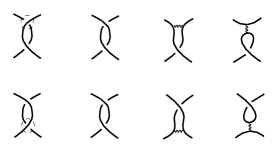
Figure 1. Top line: Details of $D_{1},D_{2},D_{3},D_{4}$; bottom line: details of $D^{\prime}_{1},D^{\prime}_{2},D^{\prime}_{3},D^{\prime}_{4}$.

∎

4. A bracket polynomial for tied link

The bracket polynonial is an invariant of regular isotopy for unoriented links introduced by Kauffman [14]. This invariant allows to define the Jones polynomial [9] trough a summation over all state diagrams of the link. A similar construction of the bracket polynomial can be done for tied links, that is, the definition is exactly the same as done by Kauffman if we restricts ourselves to crossings of a same component or between two tied components. For crossings of two untied components, a new skein relation is necessary, similar to that used in the definition of $\mathcal{L}$. In this section a Jones polynomial for tied links is also proposed.

Let $A$ and $c$ be two commutative independent variables.

Theorem 3.

There exists a unique function

$$\langle\langle\quad\rangle\rangle:\{\text{Unoriented tied links diagrams }\}\rightarrow\mathbb{Z}[A^{\pm 1},c]$$

defined by the following rules:

1. $\langle\langle\put(6.0,4.0){\circle{8.0}}\quad\rangle\rangle=1$,

2. $\langle\langle\put(6.0,4.0){\circle{8.0}}\quad\sqcup D\rangle\rangle=c\ \langle\langle\ D\ \rangle\rangle$,

3. $\langle\langle\put(6.0,4.0){\circle{8.0}}\quad\ \widetilde{\sqcup}\ D\rangle\rangle=-(A^{2}+A^{-2})\langle\langle\ D\ \rangle\rangle$,

4. $\langle\langle\quad\rangle\rangle$ is invariant under Reidemeister moves II and III,

Proof.

If all components are tied together, we can forget rules (ii) and (vi); further, observe that the remaining rules coincide with the defining rules of the bracket polynomial, where a tie is added between the strands. Then the proof follows from [14, Lemmas 2.3, 2.4 and Proposition 2.5]. Observe also that, in this case, item (iv), i.e. the invariance under Reidemeister moves II and III, can be deduced from the other rules. In the absence of ties, the invariance under Reidemeister moves II and III must be stated and its consistency with the other rules must be proved. This is done exactly as in the proof of Theorem 1, i.e., by using skein rule (vi), where $z$ is substituted by $(A+A^{-1})$. ∎

The next proposition, as well as its proof, is analogous to [14, Proposition 2.5].

Proposition 1.

The bracket polynomial $\langle\langle\quad\rangle\rangle$ satisfies:

1. $\langle\langle\includegraphics[scale={0.5},trim=0.0pt 11.38092pt 0.0pt 0.0pt]{loop1.pdf}\rangle\rangle=-A^{3}\langle\langle\includegraphics[scale={0.5},trim=0.0pt 0.0pt 0.0pt 0.0pt]{loopno.pdf}\rangle\rangle$,

2. $\langle\langle\includegraphics[scale={0.5},trim=0.0pt 11.38092pt 0.0pt 0.0pt]{loop2.pdf}\rangle\rangle=-A^{-3}\langle\langle\includegraphics[scale={0.5}]{loopno.pdf}\rangle\rangle$.

Moreover, $\langle\langle\quad\rangle\rangle$ coincides with the Kauffman bracket polynomial on classical knots and on classical links, provided that they are considered tied links whose components are all tied together.

Observe that an ambient isotopy invariant of oriented tied links can be defined in the same way as in [15, Lemma 2.1]. More precisely, we associate to every oriented link diagram $\overrightarrow{D}$, the polynomial $\mathcal{J}(\overrightarrow{D})$ defined by

(9) $$\mathcal{J}(\overrightarrow{D})=(-A)^{-3w(D)}\langle\langle D\rangle\rangle\in{\mathbb{Z}}[A^{\pm 1},c^{\pm 1}].$$

Theorem 4.

The polynomial $\mathcal{J}$ is a tie–isotopy invariant for tied links.

Corollary 1.

The polynomial $\mathcal{J}$, by the variable change $A=t^{-1/4}$, is a generalization of the Jones polynomial for tied links, that is, $\mathcal{J}$ becomes the one variable Jones polynomial on classical links, provided that they are considered tied links whose components are all tied together.

4.1. Relationship between $\langle\langle\quad\rangle\rangle$ and $\mathcal{L}$

Observe that in the same way as in [15, Proposition 3.2], we see that the polynomial $\langle\langle\quad\rangle\rangle$ is recovered from $\mathcal{L}$ by setting $a:=-A^{3}$, $z=A+A^{-1}$ and $x:=c^{-1}$. That is, for every oriented tied link diagram $\overrightarrow{D}$, we have

$$\mathcal{J}(\overrightarrow{D})=(-A)^{-3w(D)}\mathcal{L}(D)_{(a,z,x)=(-A^{3},A+A^{-1},c^{-1})}.$$

5. The tied BMW algebra

In this section we introduce a sort of tied BMW algebra, denoted by t–BMW, which plays the analogous role for the invariant $\mathcal{L}$, as the BMW algebra [5, 13] for the Kauffman polynomial $L$. This algebra is defined by generators and relations, and its defining generators have diagrammatical interpretations which are compatible with both those of the bt–algebra and the BMW–algebra. Also, in this section we prove that the t–BMW algebra is finite dimensional; this result will be crucial to demonstrate that the t–BMW algebra supports a Markov trace.

5.1.

Set ${\mathbb{K}}={\mathbb{C}}(x,z,a)$. For every $n\geq 1$, we define the tied BMW algebra, or t–BMW algebra, denoted by ${\mathcal{K}}_{n}={\mathcal{K}}_{n}(x,z,a)$, as the ${\mathbb{K}}$–algebra equal to ${\mathbb{K}}$ for $n=1$ and, for $n>1$, generated by braids generators $g_{1},\ldots,g_{n-1}$, tangles generators $h_{1},\ldots,h_{n-1}$, ties generators $e_{1},\ldots,e_{n-1}$ and tied–tangles generators $f_{1},\ldots,f_{n-1}$ subject to the following relations.

$A$–braid relations among the $g_{i}$’s:

(10) $$g_{i}g_{j} = g_{j}g_{i}\quad\text{for}\quad|i-j|>1,$$

(11) $$g_{i}g_{j}g_{i} = g_{j}g_{i}g_{j}\quad\text{for}\quad|i-j|=1.$$

BMW–relations:

(12) $$h_{i}^{2} = x^{-1}h_{i}\qquad\text{ for all }i,$$

(13) $$h_{i}h_{j} = h_{j}h_{i}\quad\text{for}\quad|i-j|>1,$$

(14) $$g_{i}h_{j} = h_{j}g_{i}\quad\text{for}\quad|i-j|>1,$$

(15) $$g_{i}h_{i} = h_{i}g_{i}=a^{-1}h_{i}\qquad\text{ for all }i,$$

(16) $$h_{i}g_{j}h_{i} = ah_{i}\quad\text{for}\quad|i-j|=1,$$

(17) $$h_{i}h_{j}h_{i} = h_{i}\qquad\text{for}\quad|i-j|=1,$$

(18) $$g_{i}g_{j}h_{i} = h_{j}g_{i}g_{j}\quad=\quad h_{j}h_{i}\qquad\text{for}\quad|i-j|=1,$$

(19) $$g_{i}h_{j}g_{i} = g_{j}^{-1}h_{i}g_{j}^{-1}\qquad\text{for}\quad|i-j|=1,$$

(20) $$g_{i}h_{j}h_{i} = g_{j}^{-1}h_{i}\qquad\text{for}\quad|i-j|=1,$$

(21) $$h_{i}h_{j}g_{i} = h_{i}g_{j}^{-1}\qquad\text{for}\quad|i-j|=1.$$

Tied braid relations:

(22) $$e_{i}e_{j} = e_{j}e_{i}\qquad\text{ for all }i,j,$$

(23) $$e_{i}^{2} = e_{i}\qquad\text{ for all }i,$$

(24) $$e_{i}g_{i} = g_{i}e_{i}\qquad\text{ for all }i,$$

(25) $$e_{i}g_{j} = g_{j}e_{i}\qquad\text{ for }|i-j|>1,$$

(26) $$e_{i}e_{j}g_{i} = g_{i}e_{i}e_{j}\quad=\quad e_{j}g_{i}e_{j}\qquad\text{ for }|i-j|=1,$$

(27) $$e_{i}g_{j}g_{i} = g_{j}g_{i}e_{j}\qquad\text{ for }|i-j|=1.$$

New relations:

(28) $$e_{i}h_{i} = h_{i}e_{i}\quad=\quad h_{i}\qquad\text{ for all }i,$$

(29) $$e_{i}h_{j} = h_{j}e_{i}\qquad\text{ for }|i-j|>1,$$

(30) $$f_{i}e_{i} = e_{i}f_{i}\quad=\quad f_{i}\qquad\text{ for all }i,$$

(31) $$f_{i}e_{j} = e_{j}f_{i}\quad=\quad e_{j}h_{i}e_{j}\qquad\text{for}\quad|i-j|=1,$$

(32) $$f_{i}g_{i} = g_{i}f_{i}\quad=\quad a^{-1}f_{i}\qquad\text{ for all }i,$$

(33) $$g_{i}f_{j}g_{i} = g_{j}^{-1}f_{i}g_{j}^{-1}\qquad\text{for}\quad|i-j|=1,$$

(34) $$g_{i}+g_{i}^{-1} = z(e_{i}+f_{i})\qquad\text{ for all }i.$$

The relations above imply:

(35) $$g_{i}^{2} = z(e_{i}g_{i}+a^{-1}f_{i})-1\text{ for all }i,$$

(36) $$f_{i}^{2} = y\ f_{i}\qquad\text{ for all }i,$$

(37) $$f_{i}h_{i} = h_{i}f_{i}\quad=\quad y\ h_{i}\qquad\text{ for all }i,$$

(38) $$e_{i}g_{j}g_{i}^{-1} = g_{j}g_{i}^{-1}e_{j}\qquad\text{ for $|i-j|=1$},$$

(39) $$f_{i}f_{j} = e_{j}h_{i}h_{j}e_{i}\qquad\text{for}\quad|i-j|=1,$$

(40) $$f_{i}h_{j} = e_{j}h_{i}h_{j}\qquad\text{for}\quad|i-j|=1,$$

(41) $$h_{j}f_{i} = h_{j}h_{i}e_{j}\qquad\text{for}\quad|i-j|=1,$$

(42) $$h_{i}g_{j}f_{i} = ah_{i}e_{j}\qquad\text{for}\quad|i-j|=1,$$

(43) $$f_{i}g_{j}h_{i} = ae_{j}h_{i}\qquad\text{for}\quad|i-j|=1,$$

(44) $$f_{i}g_{j}f_{i} = ae_{j}h_{i}e_{j}\qquad\text{for}\quad|i-j|=1,$$

where $y:=(a+a^{-1})z^{-1}-1$. Observe that relations (36) and (37) are obtained by using the expression of $f_{i}$ given by (34); namely

$$f_{i}^{2}=f_{i}\left(\frac{g_{i}+g_{i}^{-1}}{z}-e_{i}\right)=\frac{a^{-1}f_{i}+af_{i}}{z}-f_{i}=yf_{i}$$

follows from (32) and (30), whereas

$$f_{i}h_{i}=\left(\frac{g_{i}+g_{i}^{-1}}{z}-e_{i}\right)h_{i}=\frac{a^{-1}h_{i}+ah_{i}}{z}-h_{i}=yh_{i}$$

follows from (15 ) and (28).

5.2. Diagrams for the t–BMW algebra

The natural counterpart of a classical $n$–tangle in the context of tied links is a tied $n$–tangle, i.e., a rectangular piece of a diagram of a tied link with $n$ arcs and other closed curves in generic position, such that the arcs have $n$ end points at the top and $n$ end points at bottom of the rectangle, cf. [12]. Ties connect the curves inside the rectangle. Observe that, because of the ties’ mobility property [2, 6.3.3], the ties can lie entirely inside or outside the rectangle.

The relation of tie–isotopy is thus extended to tied tangles according to the following definition.

Definition 1.

Two tied $n$–tangles are regular tie–isotopic if, by substituting the first one, as a part of a tied link, with the second one, the regular tie–isotopy class of the tied link is preserved.

For our purpose we need to consider here only certain particular tied $n$–tangles, that we are going to introduce; later we will define an algebra of such diagrams that result naturally isomorphic to the algebra $\mathcal{K}_{n}$.

Observe that the defining generators of the t–BMW algebra consist of four sets of generators: the $g_{i}$’s, which correspond (diagrammatically) to the usual braid generators; the $h_{i}$’s, which correspond to the tangle generators of the BMW–algebra; the $e_{i}$’s, already introduced in the bt–algebra, which correspond to the ties, and finally certain news elements $f_{i}$’s. This last set of generators in fact corresponds to tangle generators with a tie connecting the up and bottom arcs.

More precisely, for every $n\geq 1$, we associate to the unity of the algebra $\mathcal{K}_{n}$ the trivial braid diagram made by $n$ parallel vertical threads and for $n>1$, and to the defining generators of ${\mathcal{K}}_{n}$ with index $i$ we associate diagrams coinciding with the identity except for the $i$–th and $(i+1)$–st strands as shown in the figure below.

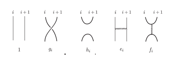
Figure 2. Diagrammatical interpretation of the defining generators of $\mathcal{K}_{n}$.

The (associative) multiplication of diagrams is defined by concatenation, i.e., the multiplication $d_{1}d_{2}$ is done by putting the diagram $d_{2}$ below of the diagram $d_{1}$.

Let $W_{n}$ be the set of diagrams obtained by translating the words in the generators of $\mathcal{K}_{n}$ generator by generator. $W_{n}$ is provided with the multiplication by concatenation. Denote ${\mathbb{K}}W_{n}$ the ${\mathbb{K}}$–vector space with basis $W_{n}$ and extend linearly the product to ${\mathbb{K}}W_{n}$. We define the algebra $\mathcal{W}_{n}$ as the ${\mathbb{K}}$–algebra constructed from ${\mathbb{K}}T_{n}$ by factoring out the defining relations of $\mathcal{K}_{n}$.

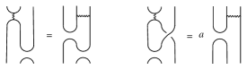
Figure 3. Relations (40) and (43).

Remark 2.

Observe that every monomial defining relation of $\mathcal{K}_{n}$, when translated to the corresponding pair of diagrams, is a relation of tie–isotopy of tied tangles, according to Definition 1 (see Fig. 3, left). Note that there are exactly five non monomial defining relations, namely relations (12), (15), (34) and the second relations in (16) and (32); an example is shown in Fig. 3, right.

In particular, the above construction defines a natural algebra isomorphism $\chi_{n}:\mathcal{K}_{n}\longrightarrow\mathcal{W}^{\prime}_{n}$, where $\mathcal{W}^{\prime}_{n}$ is the image of $\mathcal{K}_{n}$ in $\mathcal{W}_{n}$.

Remark 3.

Observe that, for every word $\alpha\in K_{n}$, the diagram $\chi_{n}(\alpha)\in\mathcal{W}^{\prime}_{n}$ can be identified with the diagram in $\mathcal{W}^{\prime}_{n+1}$, obtained by adding at right of $\chi_{n}(\alpha)$ one vertical thread. This defines a natural injective morphism of $\mathcal{W}^{\prime}_{n}$ in $\mathcal{W}^{\prime}_{n+1}$, for $n\geq 1$. We thus use the isomorphisms $\chi_{n}$’s to obtain the tower of algebras $\mathcal{K}_{1}\subset\mathcal{K}_{2}\cdots$, which is obtained by identifying, for every $n\geq 1$, $\mathcal{K}_{n}$ with the subalgebra of $\mathcal{K}_{n+1}$ generated by the defining generators of $\mathcal{K}_{n+1}$: $g_{i}$’s, $e_{i}$’s, $h_{i}$’s and $f_{i}$’s for $1\leq i\leq n-1$.

5.3. The finite dimension of the t–BMW algebra

In $\mathcal{K}_{n}$ we define the subset $\Gamma_{n}$ by

$$\Gamma_{n}:=\{1,g_{n-1},g_{n-1}e_{n-1},h_{n-1},e_{n-1},f_{n-1}\},$$

and we shall say that a word in the defining generators of $\mathcal{K}_{n}$ can be reduced, if it can be written as a linear combination of words having at most one element of $\Gamma_{n}$. Further, we say that an element in ${\mathcal{K}}_{n}$ can be reduced if it can be written as linear combination of reduced words.

Proposition 2.

Every element in ${\mathcal{K}}_{n}$ can be reduced. Thus ${\mathcal{K}}_{n}$ is finite dimensional.

To prove this proposition we need some relations and reductions which are grouped in the following lemmas.

Lemma 1.

For all $i,j$ such that $|i-j|>1$ the following relations hold:

1. $f_{i}f_{j}=f_{j}f_{i}$,

2. $f_{i}h_{j}=h_{j}f_{i}$,

3. $f_{i}g_{j}=g_{j}f_{i}$,

4. $f_{i}e_{j}=e_{j}f_{i}.$

Proof.

It is sufficient to write, by (34)

(45) $$f_{i}=z^{-1}(g_{i}+g_{i}^{-1})-e_{i}.$$

Then all relations of the lemma follow from (10), (14), (22), (24) and (25). ∎

Lemma 2.

For all $i,j$ such that $|i-j|=1$ the following relations hold:

1. $f_{i}f_{j}f_{i}=e_{j}h_{i}e_{j}$,

2. $g_{i}g_{j}f_{i}=f_{j}g_{i}g_{j}$,

3. $f_{i}f_{j}h_{i}=e_{j}h_{i}$,

4. $h_{i}f_{j}f_{i}=h_{i}e_{j}$,

5. $f_{i}f_{j}e_{i}=f_{i}f_{j}$,

6. $e_{i}f_{j}h_{i}=f_{j}h_{i}$,

7. $h_{i}f_{j}h_{i}=h_{i}$.

Proof.

Relation (i) is obtained as follows:

$$f_{i}f_{j}f_{i}=(e_{j}h_{i}h_{j}e_{i})f_{i}=e_{j}h_{i}h_{j}f_{i}=e_{j}h_{i}h_{j}h_{i}e_{j}=e_{j}h_{i}e_{j},$$

where the first to the fourth equalities are obtained, respectively, by using (39), (30), (41) and (17).

A proof of (ii) follows by expanding $f_{i}$ (see (45)) in both sides of the equality and having in mind (11) and (27).

From (40) and (30) it follows that $f_{i}f_{j}h_{i}=f_{i}e_{i}h_{j}h_{i}=f_{i}h_{j}h_{i}$. Then applying again (40) and later (17), we obtain (iii).

We prove now (iv), we have:

$$h_{i}f_{j}f_{i} = h_{i}h_{j}e_{i}f_{i}\quad\text{from (\ref{new7})}$$

$$= h_{i}h_{j}f_{i}\quad\text{from (\ref{new1})}$$

$$= h_{i}h_{j}h_{i}e_{j}\quad\text{from (\ref{new7})}$$

$$= h_{i}e_{j}\quad\text{from (\ref{bmw6})}.$$

Relation (v) is a direct consequence of (31) and (30).

Relation (vi) is a direct consequence of (31) and (28).

Relation (vii) is obtained by applying (41), then (28) and (17).

∎

Lemma 3.

The following relations hold in $\mathcal{K}_{n}$:

1. $h_{n}g_{n-1}g_{n}e_{n}=h_{n}f_{n-1}$,

2. $g_{n}e_{n}g_{n-1}h_{n}=f_{n-1}h_{n}$.

Proof.

For (i), we have:

$$h_{n}g_{n-1}g_{n}e_{n} = h_{n}h_{n-1}e_{n}\qquad\text{from}\quad(\ref{bmw7})$$

$$= h_{n}f_{n-1}\qquad\text{from}\quad(\ref{new7}).$$

For (ii), we have:

$$g_{n}e_{n}g_{n-1}h_{n} = e_{n}g_{n}g_{n-1}h_{n}\ =\ e_{n}h_{n-1}h_{n}\qquad\text{from}\quad(\ref{bmw7})$$

$$= f_{n-1}h_{n}\qquad\text{from}\quad(\ref{new6}).$$

∎

Lemma 4.

The following relations hold in $\mathcal{K}_{n}$:

1. $h_{n}f_{n-1}g_{n}=h_{n}f_{n-1}g_{n}e_{n}=h_{n}e_{n-1}g_{n-1}^{-1}$,

2. $g_{n}e_{n}f_{n-1}g_{n}=g_{n}f_{n-1}g_{n}e_{n}=g_{n}e_{n}f_{n-1}g_{n}e_{n}=g_{n-1}^{-1}e_{n-1}h_{n}e_{n-1}g_{n-1}^{-1}$,

3. $f_{n}f_{n-1}g_{n}=f_{n}f_{n-1}g_{n}e_{n}=e_{n-1}h_{n}e_{n-1}g_{n-1}^{-1}$,

4. $g_{n}f_{n-1}f_{n}=g_{n}e_{n}f_{n-1}f_{n}=g_{n-1}^{-1}e_{n-1}h_{n}e_{n-1}$,

5. $g_{n}f_{n-1}h_{n}=g_{n}e_{n}f_{n-1}h_{n}=g_{n-1}^{-1}e_{n-1}h_{n}$.

Proof.

We prove (i). We have

$$h_{n}f_{n-1}g_{n} = h_{n}h_{n-1}e_{n}g_{n}\quad\text{from (\ref{new7})}$$

$$= h_{n}h_{n-1}g_{n}e_{n}\quad\text{from (\ref{bt3})}$$

$$= h_{n}g_{n-1}^{-1}e_{n}\quad\text{from (\ref{bmw10})}$$

$$= h_{n}e_{n}g_{n-1}^{-1}e_{n}\quad\text{from (\ref{new1})}$$

$$= h_{n}e_{n}e_{n-1}g_{n-1}^{-1}\quad\text{from (\ref{bt5})}$$

$$= h_{n}e_{n-1}g_{n-1}^{-1}\quad\text{from (\ref{new1})}.$$

In the same way we prove that the second term is equal to the third term.

We prove (ii):

$$g_{n}e_{n}f_{n-1}g_{n} = g_{n}e_{n}h_{n-1}e_{n}g_{n}\quad\text{from (\ref{new9})}$$

$$= g_{n}e_{n}e_{n-1}h_{n-1}e_{n-1}e_{n}g_{n}\quad\text{from (\ref{new1})}$$

$$= e_{n}e_{n-1}g_{n}h_{n-1}g_{n}e_{n}e_{n-1}\quad\text{from (\ref{bt5})}$$

$$= e_{n}e_{n-1}g_{n-1}^{-1}h_{n}g_{n-1}^{-1}e_{n}e_{n-1}\quad\text{from (\ref{bmw8})}$$

$$= g_{n-1}^{-1}e_{n}e_{n-1}h_{n}e_{n}e_{n-1}g_{n-1}^{-1}\quad\text{from (\ref{bt5})}$$

$$= g_{n-1}^{-1}e_{n-1}h_{n}e_{n-1}g_{n-1}^{-1}\quad\text{from (\ref{new1}) and (\ref{bt1}). }$$

In the same way we prove that the second term is equal to the fourth term. By using (31), (25) and (23) we get that the third term is equal to the first: $e_{n}g_{n}f_{n-1}e_{n}g_{n}=e_{n}g_{n}e_{n}f_{n-1}g_{n}=e_{n}g_{n}f_{n-1}g_{n}$.

We prove now (iii). We have:

$$f_{n}f_{n-1}g_{n} = e_{n-1}h_{n}h_{n-1}e_{n}g_{n}\quad\text{from (\ref{new4}) }$$

$$= e_{n-1}h_{n}h_{n-1}g_{n}e_{n}\quad\text{from (\ref{bt3}) }$$

$$= e_{n-1}h_{n}g_{n-1}^{-1}e_{n}\quad\text{from (\ref{bmw10}) }$$

$$= e_{n-1}h_{n}e_{n}g_{n-1}^{-1}e_{n}\quad\text{from (\ref{new1}) }$$

$$= e_{n-1}h_{n}e_{n}e_{n-1}g_{n-1}^{-1}\quad\text{from (\ref{bt5}) }$$

$$= e_{n-1}h_{n}e_{n-1}g_{n-1}^{-1}\quad\text{from (\ref{new1}). }$$

I.e., the first term is equal to the third. Now, by using this equality we have $f_{n}f_{n-1}g_{n}e_{n}=e_{n-1}h_{n}e_{n-1}g_{n-1}^{-1}e_{n}$; but, by using (26) we have $e_{n-1}g_{n-1}^{-1}e_{n}=e_{n}e_{n-1}g_{n-1}^{-1}$, hence

$$f_{n}f_{n-1}g_{n}e_{n}=e_{n-1}h_{n}e_{n}e_{n-1}g_{n-1}^{-1}=e_{n-1}h_{n}e_{n-1}g_{n-1}^{-1},$$

where the last equality is from (28).

In analogous way we obtain (iv).

For (v), we have

$$g_{n}f_{n-1}h_{n} = g_{n}e_{n}h_{n-1}h_{n}\quad\text{from (\ref{new6})}$$

$$= e_{n}g_{n}h_{n-1}h_{n}\quad\text{from (\ref{bt3})}$$

$$= e_{n}g_{n-1}^{-1}h_{n}\quad\text{from (\ref{bmw9})}$$

$$= e_{n}g_{n-1}^{-1}e_{n}h_{n}\quad\text{from (\ref{new1})}$$

$$= g_{n-1}^{-1}e_{n-1}e_{n}h_{n}\quad\text{from (\ref{bt5}).}$$

Thus, by using now (28) we obtain $g_{n}f_{n-1}h_{n}=g_{n-1}^{-1}e_{n-1}h_{n}$. Finally, this last equality, (26) and (28) implies:

$$e_{n}g_{n}f_{n-1}h_{n}=e_{n}g_{n-1}^{-1}e_{n-1}h_{n}=g_{n-1}^{-1}e_{n-1}e_{n}h_{n}=g_{n-1}^{-1}e_{n-1}h_{n}.$$

Relation (34) implies that the words in (v) can be reduced. ∎

Lemma 5.

The following relations hold in $\mathcal{K}_{n}$:

1. $h_{n}g_{n-1}e_{n}=h_{n}e_{n-1}g_{n-1}$,

2. $e_{n}g_{n-1}h_{n}=g_{n-1}e_{n-1}h_{n}$,

3. $e_{n}g_{n-1}f_{n}=g_{n-1}e_{n-1}f_{n}$,

4. $g_{n}e_{n}g_{n-1}e_{n}=e_{n-1}g_{n}g_{n-1}e_{n-1}$,

5. $g_{n}e_{n}g_{n-1}g_{n}e_{n}=g_{n-1}g_{n}e_{n}e_{n-1}g_{n-1}$,

6. $g_{n}e_{n}g_{n-1}f_{n}=f_{n-1}g_{n}g_{n-1}e_{n-1}$.

Proof.

By using (28), we have $h_{n}g_{n-1}e_{n}=h_{n}e_{n}g_{n-1}e_{n}$, then from (26), we obtain $h_{n}g_{n-1}e_{n}=h_{n}e_{n}e_{n-1}g_{n-1}$, and using again (28), we obtain (i). Analogously, we get (ii).

For (iii) we have: $e_{n}g_{n-1}f_{n}=e_{n}g_{n-1}e_{n}f_{n}=g_{n-1}e_{n-1}e_{n}f_{n}$ since (30) and (26). Hence, (iii) follows from (30).

To obtain (iv), we use (26) and (27).

For (v), in virtue of (24), we deduce

$$g_{n}e_{n}g_{n-1}g_{n}e_{n} = g_{n}g_{n-1}e_{n}e_{n-1}g_{n}\qquad\text{from}\quad(\ref{bt6})$$

$$= g_{n}g_{n-1}g_{n}e_{n}e_{n-1}\qquad\text{from}\quad(\ref{bt5})$$

$$= g_{n-1}g_{n}g_{n-1}e_{n}e_{n-1}\qquad\text{from}\quad(\ref{b2}).$$

Then (v) follows now from (26).

To obtain (vi), observe that relation (32) implies $g_{n}e_{n}g_{n-1}f_{n}=a^{-1}g_{n}e_{n}g_{n-1}g_{n}f_{n}$. By relations (27) and (11) we get $g_{n}e_{n}g_{n-1}f_{n}=a^{-1}g_{n-1}g_{n}g_{n-1}e_{n-1}f_{n}$; now using on this last factor (31), (ii) Lemma 2 and (32), we deduce (vi).

∎

Proof of Proposition 2.

The proof is by induction on $n$. For $n=2$, the proposition follows directly from the relations (12), (15), (23), (28), (36), (37), (30), (32) and (35); thus we assume now that $n>2$. Every element in ${\mathcal{K}}_{n}$ can be written as a linear combination of elements in the form $w=w_{1}d_{1}w_{2}d_{2}\cdots w_{k}d_{k}$, where $w_{i}\in\mathcal{K}_{n-1}$ and $d_{i}\in\Gamma_{n}$. Now we shall use induction on $k$ and we see that it is enough to consider $k=2$. Hence, we are going to prove that for $w=w_{1}d_{1}w_{2}d_{2}$ the proposition holds. By the induction hypothesis we have that $w_{2}=\omega_{1}d\omega_{2}$, where $\omega_{i}\in{\mathcal{K}}_{n-2}$ and $d\in\Gamma_{n-1}$; then, $w=w_{1}\omega_{1}d_{1}dd_{2}\omega_{2}$. Thus, to finish the proof of the proposition, we need only to see that $d_{1}dd_{2}$ can be reduced in $\mathcal{K}_{n}$.

Trivially $d_{1}dd_{2}$ is reduced if $d_{1}$ or $d_{2}$ are equal to $1$. So, we consider now $d_{i}\not=1$.

For the case $d=1$, we use again (12), (15), (23), (28), (36), (37), (30), (32) and (35), to obtain $d_{1}dd_{2}$ in the reduced form. As for the remaining $125$ cases to reduce, we observe that the 50 cases obtained when $d=g_{n-1}$ and $d=f_{n-1}$ are the most representatives. We omit the analysis of the remaining cases since they can be obtained either in an analogous manner or directly from the algebra relations.

In the tables of reduction below we put in the first line the possibilities of $d_{1}$ and in the first column the possibilities of $d_{2}$ in the product $d_{1}dd_{2}$ and we will indicate how to reduce the product $d_{1}dd_{2}$.

For the case $d=g_{n-1}$, we have the following reduction table.

$$\begin{array}[]{c|ccccc}&g_{n}&h_{n}&e_{n}&g_{n}e_{n}&f_{n}\\ \hline\cr g_{n}&(\ref{b2})&(\ref{bmw7})&(\ref{bt6})&(\ref{bt6})\,\text{and}\,(\ref{b2})&\,\text{(ii) Lemma \ref{ij=1}}\\ h_{n}&(\ref{bmw7})&(\ref{bmw5})&\text{(i) Lemma \ref{L4}}&\text{(i) Lemma \ref{reductions1}}&(\ref{new11})\\ e_{n}&(\ref{bt6})&\text{(ii) Lemma \ref{L4}}&(\ref{bt5})&(\ref{bt6})&\text{(iii) Lemma \ref{L4}}\\ g_{n}e_{n}&(\ref{bt6})\,\text{and}\,(\ref{b2})&\text{(ii) Lemma \ref{reductions1}}&\text{(iv) Lemma \ref{L4}}&\text{(v) Lemma \ref{L4}}&\text{(vi) Lemma \ref{L4}}\\ f_{n}&\text{(ii) Lemma \ref{ij=1}}&(\ref{new12})&(\ref{new8})\,\text{and}\,(\ref{bt5})&\text{(ii) Lemma \ref{ij=1}\, and}\,(\ref{new9})&(\ref{new12})\\ \end{array}$$

For the case $d=f_{n-1}$, the reduction table is the following.

$$\begin{array}[]{c|ccccc}&g_{n}&h_{n}&e_{n}&g_{n}e_{n}&f_{n}\\ \hline\cr g_{n}&(\ref{new13a})\,\text{and}\,(\ref{new14})&\text{(v) Lemma \ref{reductions2}}&(\ref{new9})&\text{(ii) Lemma \ref{reductions2}}&\text{(iv) Lemma \ref{reductions2}}\\ h_{n}&\text{(i) Lemma \ref{reductions2}}&\text{(vii) Lemma \ref{ij=1} }&(\ref{new9})\,\text{and}\,(\ref{new1})&\text{(i) Lemma \ref{reductions2}}&\text{(iv) Lemma \ref{ij=1}}\\ e_{n}&(\ref{new9})&\text{(vi) Lemma \ref{ij=1}}&(\ref{new9})&(\ref{new9})&(\ref{new9})\,\text{and}\,(\ref{new8})\\ g_{n}e_{n}&\text{(ii) Lemma \ref{reductions2}}&\text{ (v) Lemma \ref{reductions2}}&(\ref{new9})&\text{(ii) Lemma \ref{reductions2}}&\text{(iv) Lemma \ref{reductions2}}\\ f_{n}&\text{(iii) Lemma \ref{reductions2}}&\text{(iii) Lemma \ref{ij=1} }&\text{(v) Lemma \ref{ij=1}}&\text{(v) Lemma \ref{ij=1} and }\,(\ref{new10})&\text{ (i) Lemma \ref{ij=1}}\end{array}$$

∎

6. A trace for the t–BMW algebra

The fact, stated in Proposition 2, that every element in ${\mathcal{K}}_{n}$ can be reduced, and the existence of the invariant $\mathcal{L}$ (Theorem 1), allow us to prove that the t–BMW algebra supports a Markov trace (see next Theorem 5). That is, we prove the existence of an unique family $\varpi=\{\varpi_{n}\}_{n\geq 1}$, where $\varpi_{n+1}:\mathcal{K}_{n+1}\rightarrow{\mathbb{K}}$ is a linear map defined from $\varpi_{n}$ and its values on $\alpha g_{n}$, $\alpha e_{n}$, $\alpha h_{n}$ and $\alpha f_{n}$, for any $\alpha\in\mathcal{K}_{n}$. We finish this section with an algebraic proof that the Kauffman polynomial $\widehat{L}$ is a specialization of the polynomial $\widehat{\mathcal{L}}$.

6.1.

Let $\alpha$ be a word in $\mathcal{K}_{n}$. In what follows we call for short closure of $\alpha$, denoted by $\widehat{\alpha}$, the closure of the image $\chi_{n}(\alpha)$ in ${\mathcal{T}}_{n}$. Observe that $\widehat{\alpha}$ is the diagram of an unoriented tied link. To prove the existence of a Markov trace on the t–BMW algebra we need the following lemma.

Lemma 6.

If the word $\alpha\in\mathcal{K}_{n}$ can be written, using the algebra relations, as a linear combination of words $\beta_{i}$, i.e., $\alpha=\sum_{i=1}^{m}k_{i}\beta_{i}$, where $k_{i}\in\mathbb{K}$, then

$$\mathcal{L}(\widehat{\alpha})=\sum_{i}k_{i}\mathcal{L}(\widehat{\beta}_{i}).$$

Proof.

Observe that in $\mathcal{K}_{n}$ every splitting of a word in a linear combination of words is done by using the basic relations (10)–(34) of the algebra. Therefore, we have firstly to prove that for every monomial relation in $\mathcal{K}_{n}$ of type $\alpha=\alpha^{\prime}$, the diagrams $\widehat{\alpha}$ and $\widehat{\alpha}^{\prime}$ are regularly isotopic, so that the value of the polynomial $\mathcal{L}$ coincides on them. Observe that relations (12),(15),(16) and (32), are considered non monomial for the presence of a coefficient different from 1. Secondly, we have to prove that for every non monomial basic relations of type $\alpha=\sum_{i}k_{i}\beta_{i}$, we have $\mathcal{L}(\widehat{\alpha})=\sum_{i}k_{i}\mathcal{L}(\widehat{\beta}_{i})$. The proof consists in a verification relation by relation and does not entail any difficulty. ∎

We define $\varpi_{1}$ as the identity; for $n>1$, $\varpi_{n}$ is given in the following theorem.

Theorem 5.

The t–BMW algebra supports a unique Markov trace $\varpi=\{\varpi_{n}\}_{n\geq 1}$, where for every positive integer $n>1$ the linear map $\varpi_{n}:\mathcal{K}_{n}\longrightarrow{\mathbb{K}}$ is defined by the following rules (recall that by definition $y=(a+a^{-1})z^{-1}-1$):

1. $\varpi_{n}(1)=1$,

2. $\varpi_{n}(\alpha\ \beta)=\varpi_{n}(\beta\ \alpha)$,

3. $\varpi_{n+1}(\alpha g_{n})=\varpi_{n+1}(\alpha g_{n}e_{n})=(x/a)\ \varpi_{n}(\alpha)$,

4. $\varpi_{n+1}(\alpha h_{n})=\varpi_{n}(\alpha f_{n})=x\ \varpi_{n}(\alpha)$,

5. $\varpi_{n+1}(\alpha e_{n})=\ x\ y\ \varpi_{n}(\alpha)$,

where $\alpha,\beta\in\mathcal{K}_{n}$.

Proof.

Given any $\alpha\in\mathcal{K}_{n}$, let $\widehat{\alpha}$ be the diagram of the unoriented tied link obtained as the closure of $\chi_{n}(\alpha)$. For every positive integer $n$, we define $\omega_{n}$ by:

(46) $$\omega_{n}(\alpha)=x^{n-1}\mathcal{L}(\widehat{\alpha}).$$

We will prove that $\omega_{n}$ satisfies (i)–(v). Since for every $n$, $\omega_{n}$ is uniquely defined, we obtain that $\varpi_{n}=\omega_{n}$ for all $n$.

We observe firstly that when $\alpha=1\in\mathcal{K}_{n}$, the closure of $\alpha$ is $\put(8.0,4.0){\circle{8.0}}\quad\,^{n}$ and, according to Theorem 1, $\mathcal{L}(\put(8.0,4.0){\circle{8.0}}\quad\,^{n})=x^{1-n}$. So, by the definition of $\omega_{n}$, we get $\omega_{n}(1)=1$. Secondly, the closures of $\alpha\beta$ and of $\beta\alpha$ are diagrams of the same tied link; therefore, by (46), $\omega_{n}(\alpha\beta)=\omega_{n}(\beta\alpha)$. Hence $\omega_{n}$ satisfies (i) and (ii).

The proof that $\omega_{n}$ satisfies (iii)–(v) is done by induction on $n$. For $n=1$, the algebra $\mathcal{K}_{1}$ contains only the unit element, i.e., the trivial braid composed of a sole thread; its closure is the circle $\put(8.0,4.0){\circle{8.0}}\quad\,^{1}$, with $\mathcal{L}(\put(8.0,4.0){\circle{8.0}}\quad\,^{1})=1$, so that $\omega_{1}(1)=1$.

We now suppose that $\omega_{j}$ satisfies (iii)–(v) for $j\leq n$. Let $\delta\in\mathcal{K}_{n+1}$. By Proposition 2, $\delta$ can be written as

$$\delta=\sum_{i=1}^{m}k_{i}\beta_{i},$$

where, for every $i$, $\beta_{i}\in\mathcal{K}_{n+1}$ contains only one element $\gamma_{i}^{(n+1)}$ of the set $\Gamma_{n+1}$, i.e.

$$\beta_{i}=\beta^{\prime}_{i}\gamma^{(n+1)}_{i}\beta^{\prime\prime}_{i},$$

where $\beta^{\prime}_{i},\beta^{\prime\prime}_{i}\in\mathcal{K}_{n}$.

Observe that, by Lemma 6, $\mathcal{L}(\hat{\delta})=\sum_{i=1}^{m}k_{i}\mathcal{L}(\hat{\beta}_{i})$. Now, for every $i$, we consider the element

$$\tilde{\beta}_{i}=\beta^{\prime\prime}_{i}\beta^{\prime}_{i}\gamma_{i}^{(n+1)}.$$

This element has the same closure as $\beta_{i}$ and then $\omega_{n+1}(\beta_{i})=\omega_{n+1}(\tilde{\beta}_{i})$. Observe that $\tilde{\beta}_{i}$ is the product of an element in $\mathcal{K}_{n}$, namely $\beta^{\prime\prime}_{i}\beta^{\prime}_{i}$, by an element in $\Gamma_{n+1}$. Therefore, it is sufficient to prove that $\omega_{n+1}$ satisfies (iii)–(v) when $\delta=\tilde{\beta}_{i}$.

Let $\alpha\in\mathcal{K}_{n}$, and $\widehat{\alpha}$ its closure, so that

$$\mathcal{L}(\widehat{\alpha})=\omega_{n}(\alpha)/x^{n-1}.$$

(iii). The closures of $\alpha g_{n}$ and of $\alpha g_{n}e_{n}$ are different from $\widehat{\alpha}$ for the presence of a new loop, and possibly of an unessential tie. Therefore, by Theorem 1,

(47) $$\mathcal{L}(\widehat{\alpha g_{n}})=\mathcal{L}(\widehat{\alpha g_{n}e_{n}})=a^{-1}\mathcal{L}(\widehat{\alpha}).$$

By (46)

$$\mathcal{L}(\widehat{\alpha g_{n}})=\omega_{n+1}(\alpha g_{n})/x^{n}\quad\text{and}\quad\mathcal{L}(\widehat{\alpha g_{n}e_{n}})=\omega_{n+1}(\alpha g_{n}e_{n})/x^{n}.$$

Therefore (47) implies

$$\omega_{n+1}(\alpha g_{n})=\omega_{n+1}(\alpha g_{n}e_{n})=xa^{-1}\omega_{n}(\alpha).$$

(iv). The closures of $\alpha h_{n}$ and of $\alpha f_{n}$ are regularly isotopic to the closure of $\alpha$, so $\mathcal{L}(\widehat{\alpha h_{n}})=\mathcal{L}(\widehat{\alpha f_{n}})=\mathcal{L}(\widehat{\alpha})$. By (46)

$$\mathcal{L}(\widehat{\alpha h_{n}})=\omega_{n+1}(\alpha h_{n})/x^{n}\quad\text{and}\quad\mathcal{L}(\widehat{\alpha f_{n}})=\omega_{n+1}(\alpha f_{n})/x^{n}.$$

Hence

$$\omega_{n+1}(\alpha h_{n})=\omega_{n+1}(\alpha f_{n})=x\omega_{n}(\alpha).$$

(v). The closure of $\alpha e_{n}$ is obtained from the closure of $\alpha$ by adding a separated circle, tied to $\widehat{\alpha}$. By (2),

(48) $$\mathcal{L}(\widehat{\alpha e_{n}})=y\mathcal{L}(\widehat{\alpha}).$$

By (46),

$$\mathcal{L}(\widehat{\alpha e_{n}})=\omega_{n+1}(\alpha e_{n})x^{n}.$$

Therefore from (48) we obtain

$$\omega_{n+1}(\alpha e_{n})=xy\omega_{n}(\alpha).$$

For completeness, we consider also the case when $\gamma_{i}^{(n+1)}$ is the identity $1_{n}\in\mathcal{K}_{n+1}$. In this case the closure of $\alpha\gamma_{i}^{(n+1)}$ is obtained from the closure of $\alpha$ by adding a separated circle. Therefore, by theorem 1, $\mathcal{L}(\widehat{\alpha 1_{n}})=\mathcal{L}(\widehat{\alpha})/x$. By (46), $\omega_{n+1}(\alpha 1_{n})=\omega_{n}(\alpha)$.

∎

Remark 4.

Observe that

(49) $$\varpi_{n+1}(\alpha g_{n}^{-1})=\varpi_{n+1}(\alpha g_{n}^{-1}e_{n})=x\ a\ \varpi_{n}(\alpha).$$

Indeed, we have

$$\alpha g_{n}^{-1}=-\alpha g_{n}+z(\alpha e_{n}+\alpha f_{n}),$$

and

$$\alpha g_{n}^{-1}e_{n}=-\alpha g_{n}e_{n}+z(\alpha e_{n}+\alpha f_{n}).$$

Now, by using (iii), (iv) and (v) we obtain:

$$\varpi_{n+1}(\alpha g_{n}^{-1})=\varpi_{n+1}(\alpha g_{n}^{-1})e_{n}=-x/a\varpi_{n}(\alpha)+z(x\ y\varpi_{n}(\alpha)+x\varpi_{n}(\alpha)=x(-a^{-1}+z(y+1))\varpi(\alpha).$$

So, $\varpi_{n}$ satisfies (49), in virtue of (3).

Remark 5.

Having present (46) and the definition of $\widehat{\mathcal{L}}$, we deduce that for the oriented tied link $\widehat{\alpha}$, with $\alpha\in TB_{n}$, we have

$$\widehat{\mathcal{L}}(\widehat{\alpha})=\left(\frac{1}{x}\right)^{n-1}a^{\rm exp(\alpha)}(\varpi_{n}\circ\pi_{n})(\alpha),$$

where $\pi_{n}$ is the representation of $TB_{n}$ defined by mapping $\sigma_{i}$ to $g_{i}$ and $\eta_{i}$ to $e_{i}$; hence, in the setting of the Jones recipe, the t–BMW algebra is the corresponding algebra to define $\widehat{\mathcal{L}}$. Now, define the tied Temperley–Lieb algebra, denoted t–${\rm TL}_{n}$, as the subalgebra of $\mathcal{K}_{n}$ generated by the $h_{i}$’s, $e_{i}$’s, and $f_{i}$’s. Notice that this subalgebra in fact can be presented abstractly through relations (12), (13), (17), (22), (23) and (28)–(31). Furthermore, note that a natural epimorphism from the tied Temperley–Lieb algebra to the classical Temperley–Lieb algebra is simply obtained by mapping $e_{i}\mapsto 1$ and $f_{i}\mapsto h_{i}$. This epimorphism and the original construction of the Jones polynomial suggest that the invariant ${\mathcal{J}}$ can be constructed through the Jones recipe applied to the algebra t–${\rm TL}_{n}$.

6.2.

In this subsection we study the factorization of $\varpi_{n}$ trough the trace on the BMW–algebra, then we re–prove that the Kauffman polynomial of oriented links corresponds to a specialization of $\widehat{\mathcal{L}}$.

Let $\ell$ and $m$ be two commutative variables. The BMW algebra ${\mathcal{C}}_{n}={\mathcal{C}}_{n}(\ell,m)$ was introduced by J. Birman and H. Wenzl [5, Section 2] and independently by J. Murakami [13]. This algebra is defined through a presentation with braid generators, tangles generators and relations among them that are motivated by topological reasons. We consider here the reduced presentation of this algebra defined in [7, Definition 1]; more precisely, ${\mathcal{C}}_{n}$ is the ${\mathbb{C}}(\ell,m)$–algebra defined through braid generators $G_{1},\ldots,G_{n-1}$ and tangle generators $H_{1},\ldots,H_{n-1}$, subject to braid relations among the $G_{i}$’s and the following relations:

(50) $$G_{i}H_{i} = \ell^{-1}H_{i}\qquad\text{for all $i$},$$

(51) $$H_{i}G_{j}H_{i} = \ell H_{i}\qquad\text{for}\quad|i-j|=1,$$

(52) $$G_{i}+G_{i}^{-1} = m(1+H_{i})\qquad\text{for all $i$}.$$

In [5, Theorem 3.2], cf. [10, Subsection 9.6], is proved that the family $\{{\mathcal{C}}_{n}\}_{n\in{\mathbb{Z}}_{>0}}$ supports a Markov trace $\tau^{\prime}=\{\tau_{n}^{\prime}\}_{n\in{\mathbb{Z}}_{>0}}$, where the $\tau_{n}^{\prime}$’s are linear maps defined uniquely by the axioms: $\tau_{n}^{\prime}(1)=1$ and for all $c,d\in{\mathcal{C}}_{n}$, we have $\tau_{n}^{\prime}(c\,d)=\tau_{n}^{\prime}(d\,c)$ and

(53) $$\tau_{n+1}^{\prime}(c\,G_{n}) = \frac{m}{\ell(\ell+\ell^{-1}-m)}\tau_{n}^{\prime}(c),$$

(54) $$\tau_{n+1}^{\prime}(c\,H_{n}) = \frac{m}{\ell+\ell^{-1}-m}\tau_{n}^{\prime}(c).$$

This Markov trace allows to define the Kauffman polynomial, $\widehat{L}$, in terms purely algebraic. More precisely, for the link $\overrightarrow{D}$ obtained as the closure of $\sigma\in B_{n}$, we have:

(55) $$\widehat{L}_{m,l}(\overrightarrow{D})=\left(\frac{\ell+\ell^{-1}-m}{m}\right)^{n-1}\ell^{w(D)}(\tau^{\prime}_{n}\circ\epsilon_{n})(\sigma),$$

where $\epsilon_{n}$ is the homomorphism from $B_{n}$ to ${\mathcal{C}}_{n}$ such that $\sigma_{i}\mapsto G_{i}$. Formula (55) is deduced by combining (23.1) and (24) of [5], cf. [10, Subsection 9.6].

Now, by regarding the defining relations of the BMW–algebra and relations (10), (11), (15) and (16), we deduce that there exists an epimorphism from a specialization of the t–BMW algebra in the BMW–algebra; further, this epimorphism factorize $\varpi$ by $\tau^{\prime}$. More precisely, we obtain the following proposition, that can be easily verified.

Proposition 3.

Setting $\ell=a$, $m=z$ and $x=\frac{z}{a+a^{-1}-z}$, we have that the mappings $g_{i}\mapsto G_{i}$, $e_{i}\mapsto 1$ and $h_{i},f_{i}\mapsto H_{i}$ define an epimorphism, denoted by $\psi_{n}$, of ${\mathbb{K}}$–algebras from $\mathcal{K}_{n}(x,z,a)$ to $\mathcal{C}_{n}(\ell,m)$. Moreover, we have $\tau_{n}^{\prime}\circ\psi_{n}=\varpi_{n}.$

Under the hypothesis of Proposition 3 we have that the following diagram is commutative:

(56)

where $\tilde{\epsilon}_{n}$ is the homomorphism from $EB_{n}$ to $\mathcal{K}_{n}$ defined by mapping $\eta^{n}\sigma_{i}\mapsto e^{n}g_{i}$, and $e^{n}:=e_{1}\cdots e_{n-1}$.

Proposition 4.

The Kauffman polynomial $\widehat{L}$ can be obtained as a specialization of the polynomial $\widehat{\mathcal{L}}$. More precisely, for an oriented tied–link $\overrightarrow{D}$ whose components are all tied together, we have

$$\widehat{\mathcal{L}}(\overrightarrow{D})=\widehat{L}(\overrightarrow{D}^{\nsim}).$$

Proof.

Theorem 2 says that $\widehat{\mathcal{L}}(\overrightarrow{D})=a^{-w(D)}\mathcal{L}(D)$. Let $\eta^{n}\sigma\in EB_{n}$ whose closure is $\overrightarrow{D}$; then from (46) we have

$$\widehat{\mathcal{L}}(\overrightarrow{D})=a^{-w(D)}x^{1-n}\varpi(\tilde{\epsilon}_{n}(\eta^{n}\sigma)).$$

Now, from the diagram above, we have:

$$\varpi(\tilde{\epsilon}_{n}(\eta^{n}\sigma)) = (\varpi\circ\tilde{\epsilon_{n}})(\eta^{n}\sigma)$$

$$= ((\tau_{n}^{\prime}\circ\psi_{n})\circ\tilde{\epsilon}_{n})(\eta^{n}\sigma)$$

$$= (\tau_{n}^{\prime}\circ(\psi_{n}\circ\tilde{\epsilon}_{n}))(\eta^{n}\sigma)$$

$$= (\tau_{n}^{\prime}\circ\epsilon_{n}\circ\mathtt{f}_{n})(\eta^{n}\sigma)$$

$$= (\tau_{n}^{\prime}\circ\epsilon_{n})(\mathtt{f}_{n}(\eta^{n}\sigma))=(\tau_{n}^{\prime}\circ\epsilon_{n})(\sigma).$$

Recall that $w(D)={\rm exp}(\overrightarrow{D})$ and $x=\frac{z}{a+a^{-1}-z}$. Therefore:

$$\widehat{\mathcal{L}}(\overrightarrow{D})=a^{-w(D)}x^{1-n}\mathcal{L}(D)=a^{-{\rm exp}(\sigma)}\left(\frac{a+a^{-1}-z}{z}\right)^{n-1}(\tau_{n}^{\prime}\circ\epsilon_{n})(\sigma)=\widehat{L}(\overrightarrow{D}^{\nsim}),$$

since $a=\ell$ and $z=m$. ∎

7. Some key examples

We give here an example of a pair of unoriented links distinguished by $\mathcal{L}$ and $\langle\langle\quad\rangle\rangle$.

Let L11n304 and L11n412 be the unoriented link diagrams obtained by forgetting the orientation in the link diagrams shown in Fig. 4 (see [6]). The calculation of $\mathcal{L}$ on these diagram gives:

$\mathcal{L}(L11n304)-\mathcal{L}(L11n412)=-z(-4z^{2}x^{2}a^{5}+zxa^{4}-3z^{2}xa^{3}+z^{3}xa^{4}+z^{3}xa^{2}+z^{2}xa+a^{3}z^{4}x-4a^{5}z^{2}x-a^{6}z^{3}x+a^{5}z^{4}x-xa^{5}-xa^{3}+a^{4}z-5z^{2}x^{2}a^{3}+z^{4}x^{2}a^{3}+z^{4}x^{2}a^{5}-z^{3}x^{2}a^{4}-a^{8}z^{3}x-2a^{6}z^{3}x^{2}+4a^{6}zx^{2}+7zx^{2}a^{4}+2zx^{2}a^{2}-a^{8}z^{3}x^{2}+2a^{7}z^{2}x^{2}-zx^{2}+a^{9}z^{2}x^{2})/(x^{2}a^{5})$

By the variable change $a:=-A^{3}$ and $z:=A-1/A$ we get:

$\langle\langle L11n304\rangle\rangle-\langle\langle L11n412\rangle\rangle=-(x^{2}+2A^{4}x+12x^{2}A^{22}+7x^{2}A^{20}+A^{30}x-A^{16}+2x^{2}A^{2}-5xA^{10}-6xA^{16}+7A^{20}x-2A^{14}+4A^{28}x+6A^{26}x+5A^{24}x-7x^{2}A^{14}-7x^{2}A^{12}-6x^{2}A^{10}-4x^{2}A^{8}-A^{12}+xA^{2}-5xA^{14}-3A^{8}x+3x^{2}A^{18}-2x^{2}A^{16}-5xA^{12}+7x^{2}A^{28}+9x^{2}A^{26}+12x^{2}A^{24}+4x^{2}A^{30}+x^{2}A^{32}-x^{2}A^{6}+x^{2}A^{4}+6A^{22}x)/(A^{17}x^{2}).$

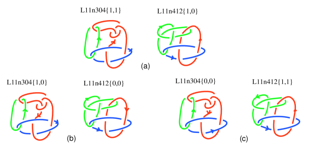
Figure 4.

Observe that the oriented links of the pair: ( L11n304{1,1},   L11n412{1,0}), shown in Fig. 4(a), have the same Homflypt polynomial, and Kauffman polynomial (see [6]). The same is true for the pairs (L11n304 {1,0},  L11n412{0,0}) and (L11n304 {0,0},   L11n412{1,1}), shown in Fig. 4(b) and (c).

The first pair is not distinguished neither by $\Theta$ nor by $\mathcal{F}$, the others are not distinguished by $\Theta$ (see [8]).

Since the writhes of the oriented diagrams in each pair coincide, it follows from the calculations above that these oriented pairs are distinguished by the generalized Kauffman polynomials (4) and (9).

Appendix

The following tables provide the value of $\mathcal{L}$ on simple unoriented tied links diagrams, shown in Fig. 5.

$$\begin{array}[]{|l|l| }\hline\cr&\mathcal{L}\\ \hline\cr\mathsf{L}1&1\\ \hline\cr\mathsf{L}2&(a+1/a)/z-1\\ \hline\cr\mathsf{L}3&1/x\\ \hline\cr\mathsf{L}4&(-a^{2}-1+az+z^{2}a^{2}+z^{2})/(az)\\ \hline\cr\mathsf{L}5&(-a+zxa^{2}+zx)/(xa)\\ \hline\cr\mathsf{L}6&(-a^{2}-1+az)^{2}/(z^{2}a^{2})\\ \hline\cr\mathsf{L}7&(a^{2}+1-az)/(azx)\\ \hline\cr\mathsf{L}8&1/x^{2}\\ \hline\cr\mathsf{L}9&(a^{2}+1-az-z^{2}a^{2}-z^{2})(-a^{2}-1+az)/(z^{2}a^{2})\\ \hline\cr\mathsf{L}10&(-a^{2}-1+az+z^{2}a^{2}+z^{2})/(azx)\\ \hline\cr\mathsf{L}11&(-a+zxa^{2}+zx)(a^{2}+1-az)/(zxa^{2})\\ \hline\cr\mathsf{L}12&(-a+zxa^{2}+zx)/(x^{2}a)\\ \hline\cr\mathsf{L}13&(a^{4}+2a^{2}-2a^{3}z+1-2az-3z^{2}a^{2}-2a^{4}z^{2}+2z^{3}a^{3}-2z^{2}+\\ &+2z^{3}a+z^{4}a^{4}+2z^{4}a^{2}+z^{4})/(z^{2}a^{2})\\ \hline\cr\mathsf{L}14&(a^{3}+a-a^{2}z-z^{2}a^{3}-az^{2}-zxa^{4}-2zxa^{2}+z^{2}xa^{3}+z^{3}xa^{4}+\\ &+2z^{3}xa^{2}-zx+z^{2}xa+z^{3}x)/(zxa^{2})\\ \hline\cr\mathsf{L}15&(a^{3}+a-a^{2}z-2zxa^{4}-4zxa^{2}+2z^{2}xa^{3}-2zx+\\ &+2z^{2}xa+z^{3}xa^{4}+2z^{3}xa^{2}+z^{3}x)/(zxa^{2})\\ \hline\cr\mathsf{L}16&(a^{2}-2zxa^{3}-2azx+z^{2}x^{2}a^{4}+2z^{2}x^{2}a^{2}+z^{2}x^{2})/(x^{2}a^{2})\\ \hline\cr\mathsf{L}17^{+}&(a^{4}+a^{2}-a^{3}z-3a^{4}z^{2}-2z^{2}a^{2}+z^{3}a^{3}+z^{4}a^{4}+z^{4}a^{2}+z^{3}a+z^{2})/(a^{3}z)\\ \hline\cr\mathsf{L}17^{-}&(a^{2}+1-az-2z^{2}a^{2}-3z^{2}+z^{3}a+z^{4}a^{2}+z^{4}+z^{3}a^{3}+a^{4}z^{2})/(az)\\ \hline\cr\mathsf{L}18^{+}&(a^{3}-3zxa^{4}-2zxa^{2}+z^{2}xa^{3}+z^{3}xa^{4}+z^{3}xa^{2}+z^{2}xa+zx)/(xa^{3})\\ \hline\cr\mathsf{L}18^{-}&(a-2zxa^{2}-3zx+z^{2}xa+z^{3}xa^{2}+z^{3}x+z^{2}xa^{3}+zxa^{4})/(xa)\\ \hline\cr\mathsf{L}19^{+}&(-2a^{3}-a+a^{2}z+z^{2}a^{3}+az^{2}+z)/(a^{2})\\ \hline\cr\mathsf{L}19^{-}&(-2-a^{2}+az+z^{2}a^{2}+z^{2}+a^{3}z)/a\\ \hline\cr\mathsf{L}20&(-1-a^{3}z-az+2z^{2}a^{2}+z^{3}a^{3}+z^{3}a+z^{2}-a^{4}-a^{2}+a^{4}z^{2})/(a^{2})\\ \hline\cr\mathsf{L}21^{+}&(a^{3}-a^{2}z-4z^{2}a^{3}-a^{4}z^{3}+3z^{4}a^{3}+z^{5}a^{4}+z^{5}a^{2}+2z^{4}a+\\ &+z^{3}+a-2a^{5}z^{2}-2az^{2}+z^{4}a^{5})/(za^{3})\\ \hline\cr\mathsf{L}21^{-}&(a^{2}-a^{3}z-4z^{2}a^{2}-z^{3}a+3z^{4}a^{2}+a^{3}z^{5}+az^{5}+2z^{4}a^{4}+\\ &+a^{5}z^{3}+a^{4}-2a^{4}z^{2}-2z^{2}+z^{4})/(za^{2})\\ \hline\cr\mathsf{L}22^{+}&(-z^{2}xa^{4}+3z^{3}xa^{3}+z^{4}xa^{4}+z^{4}xa^{2}+2z^{3}xa+z^{2}x+\\ &+a^{2}-2zxa^{5}-4zxa^{3}-2azx+z^{3}xa^{5})/(xa^{3})\\ \hline\cr\mathsf{L}22^{-}&(-z^{2}xa+3z^{3}xa^{2}+a^{3}z^{4}x+az^{4}x+2z^{3}xa^{4}+a^{5}z^{2}x+\\ &+a^{3}-2zxa^{4}-4zxa^{2}-2zx+z^{3}x)/(xa^{2})\\ \hline\cr\end{array}$$

$$\begin{array}[]{|l|l| }\hline\cr&\mathcal{L}\\ \hline\cr\mathsf{L}23^{+}&(-1+a^{4}+a^{2}-2a^{3}z-2a^{4}z^{2}-a^{2}z^{2}+2a^{3}z^{3}+z^{4}a^{4}+a^{2}z^{4}+az^{3}+z^{2}+\\ &-2a^{5}z+a^{5}z^{3})/(a^{3})\\ \hline\cr\mathsf{L}23^{-}&(-a^{5}+a^{3}+a-2a^{2}z-a^{3}z^{2}-2az^{2}+2a^{2}z^{3}+a^{3}z^{4}+az^{4}+a^{4}z^{3}+a^{5}z^{2}+\\ &-2z+z^{3})/(a^{2})\\ \hline\cr\mathsf{L}24^{+}&(3a^{5}+2a^{3}-2a^{4}z-4a^{5}z^{2}-3a^{3}z^{2}-a^{2}z+z+a^{4}z^{3}+z^{4}a^{5}+a^{3}z^{4}+a^{2}z^{3}+\\ &+az^{2})/(a^{4})\\ \hline\cr\mathsf{L}24^{-}&(3+2a^{2}-2az-3a^{2}z^{2}-4z^{2}-a^{3}z+a^{5}z+az^{3}+a^{2}z^{4}+z^{4}+a^{3}z^{3}+a^{4}z^{2})/a\\ \hline\cr\mathsf{L}25^{+}&(-a^{6}-a^{4}+a^{5}z+6a^{6}z^{2}+4a^{4}z^{2}-3a^{5}z^{3}-5a^{6}z^{4}-4z^{4}a^{4}-2a^{3}z^{3}+\\ &+a^{2}z^{2}+z^{2}+az^{3}+z^{5}a^{5}+z^{6}a^{6}+z^{6}a^{4}+a^{3}z^{5}+a^{2}z^{4})/(a^{5}z)\\ \hline\cr\mathsf{L}25^{-}&(-a^{2}-1+az+4a^{2}z^{2}+6z^{2}-3az^{3}-4a^{2}z^{4}-5z^{4}-2a^{3}z^{3}-a^{4}z^{2}+\\ &+a^{6}z^{2}+a^{5}z^{3}+az^{5}+a^{2}z^{6}+z^{6}+a^{3}z^{5}+z^{4}a^{4})/(az)\\ \hline\cr\mathsf{L}26^{+}&(-a^{5}+6a^{6}zx+4zxa^{4}-3a^{5}z^{2}x-5a^{6}z^{3}x-4z^{3}xa^{4}-2z^{2}xa^{3}-zxa^{2}+\\ &+zx+z^{2}xa+a^{5}z^{4}x+z^{5}xa^{6}+z^{5}xa^{4}+a^{3}z^{4}x+z^{3}xa^{2})/(xa^{5})\\ \hline\cr\mathsf{L}26^{-}&(-a+4zxa^{2}+6zx-3z^{2}xa-4z^{3}xa^{2}-5z^{3}x-2z^{2}xa^{3}-zxa^{4}+\\ &+a^{6}zx+a^{5}z^{2}x+az^{4}x+z^{5}xa^{2}+z^{5}x+a^{3}z^{4}x+z^{3}xa^{4})/(xa)\\ \hline\cr\mathsf{L}27^{+}&(-1+2a^{5}z+2a^{3}z-4a^{4}z^{2}-3a^{5}z^{3}-2a^{3}z^{3}+z^{2}+2z^{4}a^{4}+z^{5}a^{5}+\\ &+a^{3}z^{5}+a^{2}z^{4}+az^{3}+a^{6}+a^{4}-3a^{6}z^{2}+a^{6}z^{4})/(a^{4})\\ \hline\cr\mathsf{L}27^{-}&(-a^{6}+2az+2a^{3}z-4a^{2}z^{2}-2a^{3}z^{3}-3az^{3}+a^{6}z^{2}+2a^{2}z^{4}+\\ &+a^{3}z^{5}+az^{5}+z^{4}a^{4}+a^{5}z^{3}+a^{2}+1-3z^{2}+z^{4})/(a^{2})\\ \hline\cr\mathsf{L}28^{+}&(-1+3a^{4}z^{2}+3a^{7}z+3a^{5}z+az^{3}+a^{2}z^{4}+z^{2}-a^{4}-a^{6}+4a^{6}z^{2}-a^{3}z^{3}-3z^{4}a^{4}+\\ &+a^{3}z^{5}-6a^{5}z^{3}-4a^{6}z^{4}-4a^{7}z^{3}+a^{7}z^{5}+2z^{5}a^{5}+z^{6}a^{6}+z^{6}a^{4})/(a^{5})\\ \hline\cr\mathsf{L}28^{-}&(-a^{7}-a+3z+z^{5}-a^{3}-4z^{3}+3a^{3}z^{2}+4az^{2}+3a^{2}z+z^{4}a^{5}-a^{4}z^{3}+\\ &-6a^{2}z^{3}-3a^{3}z^{4}+z^{5}a^{4}+2a^{2}z^{5}-4az^{4}+a^{7}z^{2}+a^{6}z^{3}+a^{3}z^{6}+az^{6})/(a^{2})\\ \hline\cr\end{array}$$

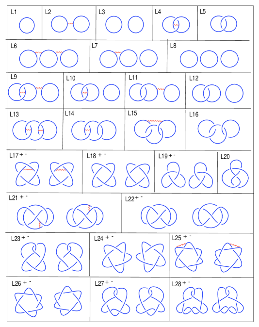
Figure 5.

References

- [1] F. Aicardi, J. Juyumaya, An algebra involving braids and ties, ICTP Preprint IC/2000/179, see also arxiv:1709.03740
- [2] F. Aicardi, J. Juyumaya, Markov trace on the algebra of braid and ties, Moscow Math. J. 16(3) (2016) 397– 431.
- [3] F. Aicardi, J. Juyumaya, Tied Links, J. Knot Theory Ramifications, 25 (2016), no. 9, DOI: 10.1142/S02182165164100171.
- [4] F. Aicardi, New invariants of links from a skein invariant of colored links, see arXiv:1512.00686
- [5] J.S. Birman, and H. Wenzl, Braids, links polynomials and a new algebra, Trans. Amer. Math. Soc., 313 (1989), no. 1, 249–273.
- [6] J. C. Cha, C. Livingston, LinkInfo: Table of Knot Invariants, http://www.indiana.edu/ linkinfo, April 16, 2015.
- [7] A.M. Cohen et al., BMW algebras of simply laced type, J. Algebra 286 (2005) 107–153.
- [8] M. Chlouveraki et al., Identifying the invariants for classical knots and links from the Yokonuma–Hecke algebras. http://arxiv.org/pdf/1505.06666.
- [9] V.F.R. Jones, Hecke algebra representations of braid groups and link polynomials, Ann. Math. 126 (1987), 335–388.
- [10] V.F.R. Jones, Subfactors and Knots, CBMS Regional Conference Series in Mathematics, Amer. Math. Soc. 80 (1991), 113 pp.
- [11] W.B.R. Lickorish, An Introduction to Knot Theory, Graduate texts in Mathematics 175, Springer (1991).
- [12] H. Morton and A. Wassermann,A basis for the Birman–Wenzl algebra, unpublished manuscript, 1989, revised 2000, 29 pp.
- [13] J. Murakami, The Kauffman polynomial of links and representation theory, Osaka J. Math., 24 (1987), 745–758.
- [14] L. Kauffman, States model and the Jones polynomial, Topology, 26 (1987), no. 3, 395–407.
- [15] L. Kauffman, An invariant of regular isotopy, Trans. Am. Math. Soc., 318 (1990), no.2, 417–471.